Metastability and dispersive shock waves in Fermi-Pasta-Ulam system

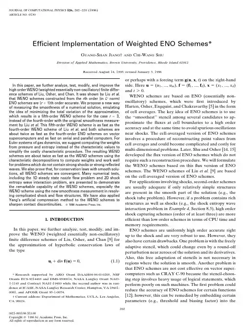
JOURNAL OF COMPUTATIONAL PHYSICS126,202–228(1996)ARTICLE NO.0130Efficient Implementation of Weighted ENO Schemes*G UANG-S HAN J IANG†AND C HI-W ANG S HUDi v ision of Applied Mathematics,Brown Uni v ersity,Pro v idence,Rhode Island02912Received August14,1995;revised January3,1996or perhaps with a forcing term g(u,x,t)on the right-handside.Here uϭ(u1,...,u m),fϭ(f1,...,f d),xϭ(x1,...,x d) In this paper,we further analyze,test,modify,and improve thehigh order WENO(weighted essentially non-oscillatory)finite differ-and tϾ0.ence schemes of Liu,Osher,and Chan.It was shown by Liu et al.WENO schemes are based on ENO(essentially non-that WENO schemes constructed from the r th order(in L1norm)oscillatory)schemes,which werefirst introduced by ENO schemes are(rϩ1)th order accurate.We propose a new wayHarten,Osher,Engquist,and Chakravarthy[5]in the form of measuring the smoothness of a numerical solution,emulatingthe idea of minimizing the total variation of the approximation,of cell averages.The key idea of ENO schemes is to use which results in afifth-order WENO scheme for the case rϭ3,the‘‘smoothest’’stencil among several candidates to ap-instead of the fourth-order with the original smoothness measure-proximate thefluxes at cell boundaries to a high order ment by Liu et al.Thisfifth-order WENO scheme is as fast as theaccuracy and at the same time to avoid spurious oscillations fourth-order WENO scheme of Liu et al.and both schemes arenear shocks.The cell-averaged version of ENO schemes about twice as fast as the fourth-order ENO schemes on vectorsupercomputers and as fast on serial and parallel computers.For involves a procedure of reconstructing point values from Euler systems of gas dynamics,we suggest computing the weights cell averages and could become complicated and costly for from pressure and entropy instead of the characteristic values to multi-dimensional ter,Shu and Osher[14,15] simplify the costly characteristic procedure.The resulting WENOdeveloped theflux version of ENO schemes which do not schemes are about twice as fast as the WENO schemes using thecharacteristic decompositions to compute weights and work well require such a reconstruction procedure.We will formulate for problems which do not contain strong shocks or strong reflected the WENO schemes based on thisflux version of ENO waves.We also prove that,for conservation laws with smooth solu-schemes.The WENO schemes of Liu et al.[9]are basedtions,all WENO schemes are convergent.Many numerical tests,on the cell-averaged version of ENO schemes.including the1D steady state nozzleflow problem and2D shockFor applications involving shocks,second-order schemes entropy wave interaction problem,are presented to demonstratethe remarkable capability of the WENO schemes,especially the are usually adequate if only relatively simple structures WENO scheme using the new smoothness measurement in resolv-are present in the smooth part of the solution(e.g.,the ing complicated shock andflow structures.We have also applied shock tube problem).However,if a problem contains rich Yang’s artificial compression method to the WENO schemes tostructures as well as shocks(e.g.,the shock entropy wave sharpen contact discontinuities.ᮊ1996Academic Press,Inc.interaction problem in Example4,Section8.3),high ordershock capturing schemes(order of at least three)are more1.INTRODUCTION efficient than low order schemes in terms of CPU time andmemory requirements.In this paper,we further analyze,test,modify,and im-ENO schemes are uniformly high order accurate rightprove the WENO(weighted essentially non-oscillatory)up to the shock and are very robust to use.However,theyfinite difference schemes of Liu,Osher,and Chan[9]for also have certain drawbacks.One problem is with the freelythe approximation of hyperbolic conservation laws of adaptive stencil,which could change even by a round-offthe type perturbation near zeroes of the solution and its derivatives.Also,this free adaptation of stencils is not necessary in u tϩdiv f(u)ϭ0,(1.1)regions where the solution is smooth.Another problem isthat ENO schemes are not cost effective on vector super-computers such as CRAY C-90because the stencil-choos-*Research supported by ARO Grant DAAH04-94-G-0205,NSFGrants ECS-9214488and DMS-9500814,NASA Langley Grant NAG-ing step involves heavy usage of logical statements,which 1-1145and Contract NAS1-19480while the second author was in resi-perform poorly on such machines.Thefirst problem could dence at ICASE,NASA Langley Research Center,Hampton,VA23681-reduce the accuracy of ENO schemes for certain functions 0001,and AFOSR Grant95-1-0074.[12];however,this can be remedied by embedding certain †Current address:Department of Mathematics,UCLA,Los Angeles,CA90024.parameters(e.g.,threshold and biasing factor)into the2020021-9991/96$18.00Copyright©1996by Academic Press,Inc.All rights of reproduction in any form reserved.WEIGHTED ENO SCHEMES203 stencil choosing step so that the preferred linearly stable the total variation of the approximations.This new mea-surement gives the optimalfifth-order accurate WENO stencil is used in regions away from discontinuities.See[1,3,13].scheme when rϭ3(the smoothness measurement in[9]gives a fourth-order accurate WENO scheme for rϭ3). The WENO scheme of Liu,Osher,and Chan[9]is an-other way to overcome these drawbacks while keeping the Although the WENO schemes are faster than ENOschemes on vector supercomputers,they are only as fast robustness and high order accuracy of ENO schemes.Theidea is the following:instead of approximating the numeri-as ENO schemes on serial computers.In Section4,wepresent a simpler way of computing the weights for the calflux using only one of the candidate stencils,one usesa con v ex combination of all the candidate stencils.Each approximation of Euler systems of gas dynamics.The sim-plification is aimed at reducing thefloating point opera-of the candidate stencils is assigned a weight which deter-mines the contribution of this stencil to thefinal approxi-tions in the costly but necessary characteristic procedureand is motivated by the following observation:the only mation of the numericalflux.The weights can be definedin such a way that in smooth regions it approaches certain nonlinearity of a WENO scheme is in the computation ofthe weights.We suggest using pressure and entropy to optimal weights to achieve a higher order of accuracy(anr th-order ENO scheme leads to a(2rϪ1)th-order WENO compute the weights,instead of the local characteristicquantities.In this way one can exploit the linearity of the scheme in the optical case),while in regions near disconti-nuities,the stencils which contain the discontinuities are rest of the scheme.The resulting WENO schemes(rϭ3)is about twice as fast as the original WENO scheme which assigned a nearly zero weight.Thus essentially non-oscilla-tory property is achieved by emulating ENO schemes uses local characteristic quantities to compute the weights(see Section7).The same idea can also be applied to the around discontinuities and a higher order of accuracy isobtained by emulating upstream central schemes with the original ENO ly,we can use the undivideddifferences of pressure and entropy to replace the local optimal weights away from the discontinuities.WENOschemes completely remove the logical statements that characteristic quantities to choose the ENO stencil.Thishas been tested numerically but the results are not included appear in the ENO stencil choosing step.As a result,theWENO schemes run at least twice as fast as ENO schemes in this paper since the main topic here is the WENOschemes.(see Section7)on vector machines(e.g.,CRAY C-90)andare not sensitive to round-off errors that arise in actual WENO schemes have the same smearing at contact dis-continuities as ENO schemes.There are mainly two tech-computation.Atkins[1]also has a version of ENO schemesusing a different weighted average of stencils.niques for sharpening the contact discontinuities for ENOschemes.One is Harten’s subcell resolution[4]and the Another advantage of WENO schemes is that itsflux issmoother than that of the ENO schemes.This smoothness other is Yang’s artificial compression(slope modification)[20].Both were introduced in the cell average context. enables us to prove convergence of WENO schemes forsmooth solutions using Strang’s technique[18];see Section Later,Shu and Osher[15]translated them into the pointvalue framework.In one-dimensional problems,the sub-6.According to our numerical tests,this smoothness alsohelps the steady state calculations,see Example4in Sec-cell resolution technique works slightly better than theartificial compression method.However,for two or higher tion8.2.In[9],the order of accuracy shown in the error tables dimensional problems,the latter is found to be more effec-tive and handy to use[15].We will highlight the key proce-(Table1–5in[9])seemed to suggest that the WENOschemes of Liu et al.are more accurate than what the dures of applying the artificial compression method to theWENO schemes in Section5.truncation error analysis indicated.In Section2,we carryout a more detailed error analysis for the WENO schemes In Section8,we test the WENO schemes(both theWENO schemes of Liu et al.and the modified WENO andfind that this‘‘super-convergence’’is indeed superfi-cial:the‘‘higher’’order is caused by larger error on the schemes)on several1D and2D model problems and com-pare them with ENO schemes to examine their capability coarser grids instead of smaller error on thefiner grids.Our error analysis also suggests that the WENO schemes in resolving shock and complicatedflow structures.We conclude this paper by a brief summary in Section can be made more accurate than those in[9].Since the weight on a candidate stencil has to vary ac-9.The time discretization of WENO schemes will be imple-mented by a class of high order TVD Runge–Kutta-type cording to the relative smoothness of this stencil to theother candidate stencils,the way of evaluating the smooth-methods developed by Shu and Osher[14].To solve theordinary differential equationness of a stencil is crucial in the definition of the weight.In Section3,we introduce a new way of measuring thesmoothness of the numerical solution which is based uponminimizing the L2norm of the derivatives of the recon-dudt ϭL(u),(1.2)struction polynomials,emulating the idea of minimizing204JIANG AND SHUTABLE I where L (u )is a discretization of the spatial operator,the third-order TVD Runge–Kutta is simplyCoefficients a r k ,lrk l ϭ0l ϭ1l ϭ2u (1)ϭu n ϩ⌬tL (u n )u (2)ϭ u n ϩ u (1)ϩ ⌬tL (u (1))(1.3)20Ϫ1/23/211/21/2u n ϩ1ϭ u n ϩ u (2)ϩ ⌬tL (u (2)).301/3Ϫ7/611/61Ϫ1/65/61/3Another useful,although not TVD,fourth-order Runge–21/35/6Ϫ1/6Kutta scheme isu (1)ϭu n ϩ ⌬tL (u n )f (u )ϭf ϩ(u )ϩf Ϫ(u ),(2.4)u(2)ϭu nϩ ⌬tL (u (1))(1.4)where df (u )ϩ/du Ն0and df (u )Ϫ/du Յ0.For example,u (3)ϭu n ϩ⌬tL (u (2))one can defineu n ϩ1ϭ (Ϫu n ϩu (1)ϩ2u (2)ϩu (3))ϩ ⌬tL (u (3)).f Ϯ(u )ϭ (f (u )ϮͰu ),(2.5)This fourth-order Runge–Kutta scheme can be made TVD by an increase of operation counts [14].We will mainly where Ͱϭmax ͉f Ј(u )͉and the maximum is taken over the use these two Runge–Kutta schemes in our numerical tests whole relevant range of u .This is the global Lax–Friedrichs in Section 8.The third-order TVD Runge–Kutta scheme (LF)flux splitting.For other flux splitting,especially the will be referred to as ‘‘RK-3’’while the fourth-order (non-Roe flux splitting with entropy fix (RF);see [15]for details.TVD)Runge–Kutta scheme will be referred to as ‘‘RK-4.’’Let f ˆϩj ϩ1/2and f Ϫj ϩ1/2be,resp.the numerical fluxes obtained from the positive and negative parts of f (u ),we then have2.THE WENO SCHEMES OF LIU,OSHER,AND CHANf ˆj ϩ1/2ϭf ˆϩj ϩ1/2ϩf ˆϪj ϩ1/2.(2.6)In this section,we use the flux version of ENO schemes Here we will only describe how f ˆϩj ϩ1/2is computed in [9]as our basis to formulate WENO schemes of Liu et al.and on the basis of flux version of ENO schemes.For simplicity,analyze their accuracy in a different way from that used we will drop the ‘‘ϩ’’sign in the superscript.The formulas in [9].We use one-dimensional scalar conservation laws for the negative part of the split flux are symmetric (with (i.e.,d ϭm ϭ1in (1.1))as an example:respect to x j ϩ1/2)and will not be shown.As we know,the r th-order (in L 1sense)ENO scheme u t ϩf (u )x ϭ0.(2.1)chooses one ‘‘smoothest’’stencil from r candidate stencils and uses only the chosen stencil to approximate the flux Let us discretize the space into uniform intervals of sizeh j ϩ1/2.Let’s denote the r candidate stencils by S k ,k ϭ0,⌬x and denote x j ϭj ⌬x .Various quantities at x j will be 1,...,r Ϫ1,whereidentified by the subscript j .The spatial operator of the WENO schemes,which approximates Ϫf (u )x at x j ,will S k ϭ(x j ϩk Ϫr ϩ1,x j ϩk Ϫr ϩ2,...,x j ϩk ).take the conservative formIf the stencil S k happens to be chosen as the ENO interpola-L ϭϪ1⌬x(f ˆj ϩ1/2Ϫf ˆj Ϫ1/2),(2.2)tion stencil,then the r th-order ENO approximation of h j ϩ1/2iswhere the numerical flux f ˆj ϩ1/2approximates h j ϩ1/2ϭf ˆj ϩ1/2ϭq r k (f j ϩk Ϫr ϩ1,...,f j ϩk ),(2.7)h (x j ϩ1/2)to a high order with h (x )implicitly defined by [15]wheref (u (x ))ϭ1⌬x͵x ϩ⌬x /2x Ϫ⌬x /2h (␰)d ␰.(2.3)q r k (g 0,...,g r Ϫ1)ϭ͸r Ϫ1l ϭ0ark ,l g l .(2.8)Here a r k ,l ,0Յk ,l Յr Ϫ1,are constant coefficients.For We can actually assume f Ј(u )Ն0for all u in the range of our interest.For a general flux,i.e.,f Ј(u )Ն͞0,one can later use,we provide these coefficients for r ϭ2,3,in Table I.split it into two parts either globally or locally,WEIGHTED ENO SCHEMES205TABLE II To just use the one smoothest stencil among the r candi-dates for the approximation of h j ϩ1/2,is very desirable nearOptimal Weights C r kdiscontinuities because it prohibits the usage of informa-C r k k ϭ0k ϭ1k ϭ2tion on discontinuous stencils.However,it is not so desir-able in smooth regions because all the candidate stencils r ϭ21/32/3—carry equally smooth information and thus can be used r ϭ31/106/103/10together to give a higher order (higher than r ,the order of the base ENO scheme)approximation to the flux h j ϩ1/2.In fact,one could use all the r candidate stencils,which all together contain (2r Ϫ1)grid values of f to give f ˆj ϩ1/2ϭq 2r Ϫ1r Ϫ1(f j Ϫr ϩ1,...,f j ϩr Ϫ1)(2.12)a (2r Ϫ1)th-order approximation of h j ϩ1/2:ϩ͸r Ϫ1k ϭ0(ͶkϪC r k )q rk (f j ϩk Ϫr ϩ1,...,f j ϩk ).f ˆj ϩ1/2ϭq 2r Ϫ1r Ϫ1(f j Ϫr ϩ1,...,f j ϩr Ϫ1)(2.9)Recalling (2.9),we see that,the first term on the right-which is just the numerical flux of a (2r Ϫ1)th-order up-hand side of the above equation is a (2r Ϫ1)th-orderstream central scheme.As we know,high order upstreamapproximation of h j ϩ1/2.Since ͚r Ϫ1k ϭ0C r k ϭ1,if we require central schemes (in space),combined with high order ͚r Ϫ1k ϭ0Ͷk ϭ1,the last summation term can be written asRunge–Kutta methods (in time),are stable and dissipative under appropriate CFL numbers and thus are convergent,according to Strang’s convergence theory [18]when the ͸r Ϫ1k ϭ0(ͶkϪC r k)(q r k(fj ϩk Ϫr ϩ1,...,f j ϩk )Ϫh j ϩ1/2).(2.13)solution of (1.1)is smooth (see Section 6).The above facts suggest that one could use the (2r Ϫ1)th-order upstream central scheme in smooth regions and only use the r th-Each term in the last summation can be made O (h 2r Ϫ1)iforder ENO scheme near discontinuities.As in (2.7),each of the stencils can render an approxima-Ͷk ϭC r k ϩO (hr Ϫ1)(2.14)tion of h j ϩ1/2.If the stencil is smooth,this approximation is r th-order accurate;otherwise,it is less accurate or even for k ϭ0,1,...,r Ϫ1.Here,h ϭ⌬x .Thus C r k will bearnot accurate at all if the stencil contains a discontinuity.the name of optimal weight.One could assign a weight Ͷk to each candidate stencil S k ,The question now is how to define the weight such that k ϭ0,1,...,r Ϫ1,and use these weights to combine the (2.14)is satisfied in smooth regions while essentially non-r different approximations to obtain the final approxima-oscillatory property is achieved.In [9],the weight Ͷk for tion of h j ϩ1/2asstencil S k is defined byͶk ϭͰk0r Ϫ1,(2.15)fˆj ϩ1/2ϭ͸r Ϫ1k ϭ0Ͷk q r k (f j ϩk Ϫr ϩ1,...,f j ϩk ),(2.10)wherewhere q r k (f j ϩk Ϫr ϩ1,...,f j ϩk )is defined in (2.8).To achieveessentially non-oscillatory property,one then requires the weight to adapt to the relative smoothness of f on each Ͱk ϭC r k(␧ϩIS k )p,k ϭ0,1,...,r Ϫ1.(2.16)candidate stencil such that any discontinuous stencil is ef-fectively assigned a zero weight.In smooth regions,one Here ␧is a positive real number number which is intro-can adjust the weight distribution such that the resultingduced to avoid the denominator becoming zero (in our approximation of the flux fˆj ϩ1/2is as close as possible to later tests,we will take ␧ϭ10Ϫ6.Our numerical tests that given in (2.9).indicate that the result is not sensitive to the choice of ␧,Simple algebra gives the coefficients C r k such thatas long as it is in the range of 10Ϫ5to 10Ϫ7);the power p will be discussed in a moment;IS k in (2.16)is a smoothness measurement of the flux function on the k th candidate q 2r Ϫ1r Ϫ1(f j Ϫr ϩ1,...,f j ϩr Ϫ1)ϭ͸r Ϫ1k ϭ0C r k q rk(fj ϩk Ϫr ϩ1,...,f j ϩk )(2.11)stencil.It is easy to see that ͚r Ϫ1k ϭ0Ͷk ϭ1.To satisfy (2.14),it suffices to have (through a Taylor expansion analysis)and ͚r Ϫ1k ϭ0C r k ϭ1for all r Ն2.For r ϭ2,3,these coefficients are given in Table II.Comparing (2.11)with (2.10),we getIS k ϭD (1ϩO (h r Ϫ1))(2.17)206JIANG AND SHUfor k ϭ0,1,...,r Ϫ1,where D is some non-zero quantity IS 1ϭ ((f Јh Ϫ f Љh 2)2ϩ(f Јh ϩ f Љh 2)2)independent of k .As we know,an ENO scheme chooses the ‘‘smoothest’’ϩ(f Љh 2)2ϩO (h 5)(2.24)ENO stencil by comparing a hierarchy of undivided differ-IS 2ϭ ((f Јh ϩ f Љh 2)2ϩ(f Јh ϩ f Љh 2)2)ences.This is because these undivided differences can be used to measure the smoothness of the numerical flux on ϩ(f Љh 2)2ϩO (h 5).(2.25)a stencil.In [9],IS k is defined asWe can see that the second-order terms are different from stencil to stencil.Thus (2.22)is no longer valid at critical IS k ϭ͸r Ϫ1l ϭ1͸r Ϫli ϭ1(f [j ϩk ϩi Ϫr ,l ])2r Ϫl,(2.18)points of f (u (x ))which implies that the WENO scheme of Liu et al.for r ϭ3is only third-order accurate at these points.In fact,the weights computed from the smoothness where f [и,и]is the l th undivided difference:measurement (2.18)diverge far away from the optimal weights near critical points (see Fig.1in the next section)f [j ,0]ϭf jon coarse grids (10to 80grid points per wave).But on f [j ,l ]ϭf [j ϩ1,l Ϫ1]Ϫf [j ,l Ϫ1],k ϭ1,...,r Ϫ1.fine grids,since the smoothness measurements IS k for all k are relatively smaller than the non-zero constant ␧in For example,when r ϭ2,we have(2.16),the weights become close to the optimal weights.Therefore the ‘‘super-convergence’’phenomena appeared IS k ϭ(f [j ϩk Ϫ1,1])2,k ϭ0,1.(2.19)in Tables 1–5in [9]are caused by large error commitment on coarse grids and less error commitment on finer grids When r ϭ3,(2.18)giveswhen using the errors of the fifth-order central scheme as reference (see Tables III and IV).IS k ϭ ((f [j ϩk Ϫ2,1])2ϩ(f [j ϩk Ϫ1,1])2)(2.20)At discontinuities,it is typical that one or more of the r candidate stencils reside in smooth regions of the numerical ϩ(f [j ϩk Ϫ2,2])2,k ϭ0,1,2.solution while other stencils contain the discontinuities.The size of the discontinuities is always O (1)and does not In smooth regions,Taylor expansion analysis of (2.18)change when the grid is refined.So we have for a smooth givesstencil S k ,IS k ϭ(f Јh )2(1ϩO (h )),k ϭ0,1,...,r Ϫ1,(2.21)IS k ϭO (h 2p )(2.26)where f Јϭf Ј(u j ).Note the O (h )term is not O (h r Ϫ1)that we and for a non-smooth stencil S l ,would want to have (see (2.17)).Thus in smooth monotone regions,i.e.,f Ј϶0,we haveIS l ϭO (1).(2.27)Ͷk ϭC r k ϩO (h ),k ϭ0,1,...,r Ϫ1.(2.22)From the definition of the weights (2.15),we can see that,for this non-smooth stencil S l ,the corresponding weight Recalling (2.12),we see that the WENO schemes with theͶl satisfiessmoothness measurement given by (2.18)is (r ϩ1)th-order accurate in smooth monotone regions of f (u (x )).This re-Ͷl ϭO (h 2p ).(2.28)sult was proven in [9]using a different approach.For r ϭ2,this is optimal in the sense that the third-order upstream Therefore for small h and any positive integer power p ,central scheme is approximated in most smooth regions.the weight assigned to the non-smooth stencil vanishes as However,this is not optimal for r ϭ3,for which this h Ǟ0.Note,if there is more than one smooth stencils in measurement can only give fourth-order accuracy while the r candidates,from the definition of the weights in (2.15),the optimal upstream central scheme is fifth-order accu-we expect each of the smooth stencils will get a weight rate.We will introduce a new measurement in the next which is O (1).In this case,the weights do not exactly section which will result in an optimal order accurate resemble the ‘‘ENO digital weights.’’However,if a stencil WENO scheme for the r ϭ3case.is smooth,the information that it contains is useful and When r ϭ3,Taylor expansion of (2.20)givesshould be utilized.In fact,in our extensive numerical ex-periments,we find the WENO schemes in [9]work very IS 0ϭ ((f Јh Ϫ f Љh 2)2ϩ(f Јh Ϫ f Љh 2)2)well at shocks.We also find that p ϭ2is adequate to obtain essentially non-oscillatory approximations at leastϩ(f Љh 2)2ϩO (h 5)(2.23)WEIGHTED ENO SCHEMES207for r ϭ2,3,although it is suggested in [9]that p should IS 1ϭ (f j Ϫ1Ϫ2f j ϩf j ϩ1)2ϩ (f j Ϫ1Ϫf j ϩ1)2(3.3)be taken as r ,the order of the base ENO schemes.We will use p ϭ2for all our numerical tests.Notice that,IS 2ϭ(f j Ϫ2f j ϩ1ϩf j ϩ2)2ϩ (3f j Ϫ4f j ϩ1ϩf j ϩ2)2.(3.4)in discussing accuracy near discontinuities,we are simply concerned with spatial approximation error.The error due In smooth regions.Taylor expansion of (3.2)–(3.4)gives,to time evolution is not considered.respectively,In summary,WENO schemes of Liu et al.defined by (2.10),(2.15),and (2.18)have the following properties:IS 0ϭ (f Љh 2)2ϩ (2f Јh Ϫ f ٞh 3)2ϩO (h 6)(3.5)1.They involve no logical statements which appear in IS 1ϭ(f Љh 2)2ϩ (2f Јh ϩ f ٞh 3)2ϩO (h 6)(3.6)the base ENO schemes.IS 2ϭ (f Љh 2)2ϩ (2f Јh Ϫ f ٞh 3)2ϩO (h 6),(3.7)2.The WENO scheme based on the r th-order ENO scheme is (r ϩ1)th-order accurate in smooth monotone where f ٞϭf ٞ(u j ).If f Ј϶0,thenregions,although this is still not as good as the optimal order (2r Ϫ1).IS k ϭ(f Јh )2(1ϩO (h 2)),k ϭ0,1,2,(3.8)3.They achieve essentially non-oscillatory property by emulating ENO schemes at discontinuities.which means the weights (see (2.15))resulting from thismeasurement satisfy (2.17)for r ϭ3;thus we obtain a 4.They are smooth in the sense that the numerical flux fifth-order (the optimal order for r ϭ3)accurate f ˆj ϩ1/2is a smooth function of all its arguments (for a general WENO scheme.flux,this is also true if a smooth flux splitting method is Moreover,this measurement is also more accurate at used,e.g.,global Lax–Friedrichs flux splitting).critical points of f (u (x )).When f Јϭ0,we have3.A NEW SMOOTHNESS MEASUREMENTIS k ϭ (f Љh 2)2(1ϩO (h 2)),k ϭ0,1,2,(3.9)In this section,we present a new way of measuring thesmoothness of the numerical solution on a stencil which which implies that the weights resulting from the measure-can be used to replace (2.18)to form a new weight.As we ment (3.1)is also fifth-order accurate at critical points.know,on each stencil S k ,we can construct a (r Ϫ1)th-To illustrate the different behavior of the two measure-order interpolation polynomial,which if evaluated at x ϭments (i.e.,(2.18)and (3.1))for r ϭ3in smooth monotone x j ϩ1/2,renders the approximation of h j ϩ1/2given in (2.7).regions,near critical points or near discontinuities,we com-Since total variation is a good measurement for smooth-pute the weights Ͷ0,Ͷ1,and Ͷ2for the functionness,it would be desirable to minimize the total variation for the approximation.Consideration for a smooth flux and for the role of higher order variations leads us to the f j ϭͭsin 2ȏx j if 0Յx j Յ0.5,1Ϫsin 2ȏx j if 0.5Ͻx j Յ1.(3.10)following measurement for smoothness:let the interpola-tion polynomial on stencil S k be q k (x );we defineat all half grid points x j ϩ1/2,where x j ϭj ⌬x ,x j ϩ1/2ϭx j ϩ⌬x /2,and ⌬x ϭ .We display the weights Ͷ0and Ͷ1in IS k ϭ͸r Ϫ1l ϭ1͵x j ϩ1/2x j Ϫ1/2h 2l Ϫ1(q (l )k )2dx ,(3.1)Fig.1(Ͷ2ϭ1ϪͶ0ϪͶ1is omitted in the picture).Notethe optimal weight for Ͷ0is C 30ϭ0.1and for Ͷ1is C 31ϭ0.6.We can see that the weights computed with (2.18)where q (l )kis the l th-derivative of q k (x ).The right-hand side (referred to as the original measurement in Fig.1)are of (3.1)is just a sum of the L 2norms of all the derivatives far less optimal than those with the new measurement,of the interpolation polynomial q k (x )over the interval especially around the critical points x ϭ , .However,near (x j Ϫ1/2,x j ϩ1/2).The term h 2l Ϫ1is to remove h -dependent the discontinuity x ϭ ,the two measurements behave factors in the derivatives of the polynomials.This is similar similarly;the discontinuous stencil always gets an almost-to,but smoother than,the total variation measurement zero weight.Moreover,for the grid point immediately left based on the L 1norm.It also renders a more accurate to the discontinuity,Ͷ0Ȃ and Ͷ1Ȃ ,which means,when WENO scheme for the case r ϭ3,when used with (2.15)only one of the three stencils is non-smooth,the other two and (2.16).stencils get O (1)weights.Unfortunately,these weights do When r ϭ2,(3.1)gives the same measurement as (2.18).not approximate a fourth-order scheme at this point.A However,they become different for r Ն3.For r ϭ3,similar situation happens to the point just to the right of (3.1)givesthe discontinuity.For simplicity of notation,we use WENO-X-3to standIS 0ϭ (f j Ϫ2Ϫ2f j Ϫ1ϩf j )2ϩ (f j Ϫ2Ϫ4f j Ϫ1ϩ3f j )2(3.2)208JIANG AND SHUFIG.1.A comparison of the two smoothness measurements.for the third-order WENO scheme (i.e.,r ϭ2,for which u 0(x )ϭsin 4(ȏx ).Again we see that WENO-RF-4is more accurate than WENO-RF-5on the coarsest grid (N ϭ20)the original and new smoothness measurement coincide)but becomes less accurate than WENO-RF-5on finer grids.(where X ϭLF,Roe,RF refer,respectively,to the global The order of accuracy for WENO settles down later than Lax–Friedrichs flux splitting,Roe’s flux splitting,and Roe’s in the previous example.Notice that this is the example flux splitting with entropy fix).The accuracy of this scheme for which ENO schemes lose their accuracy [12].has been tested in [9].We will use WENO-X-4to represent the fourth-order WENO scheme of Liu et al.(i.e.,r ϭ3 4.A SIMPLE WAY FOR COMPUTING WEIGHTS FORwith the original smoothness measurement of Liu et al .)EULER SYSTEMSand WENO-X-5to stand for the fifth-order WENO scheme resulting from the new smoothness measurement.In later For system (1.1)with d Ͼ1,the derivatives d f i /dx i ,i ϭsections,we will also use ENO-X-Y to denote conventional 1,...,d ,are approximated dimension by dimension;forENO schemes of ‘‘Y’’th order with ‘‘X’’flux splitting.We caution the reader that the orders here are in L 1sense.So TABLE IIIENO-RF-4in our notation refers to the same scheme as ENO-RF-3in [15].Accuracy on u t ϩu x ϭ0with u 0(x )ϭsin(ȏx )In the following we test the accuracy of WENO schemes Method N L ȍerror L ȍorder L 1error L 1order on the linear equation:WENO-RF-410 1.31e-2—7.93e-3—u t ϩu x ϭ0,Ϫ1Յx Յ1,(3.11)20 3.00e-3 2.13 1.32e-3 2.5940 4.27e-4 2.81 1.56e-4 3.08u (x ,0)ϭu 0(x ),periodic.(3.12)80 5.17e-5 3.05 1.13e-5 3.79160 4.99e-6 3.37 6.88e-7 4.04320 3.44e-7 3.86 2.74e-8 4.65In Table III,we show the errors of the two schemes at t ϭ1for the initial condition u 0(x )ϭsin(ȏx )and compare WENO-RF-510 2.98e-2— 1.60e-2—them with the errors of the fifth-order upstream central 20 1.45e-3 4.367.41e-4 4.4340 4.58e-5 4.99 2.22e-5 5.06scheme (referred to as CENTRAL-5in the following ta-80 1.48e-6 4.95 6.91e-7 5.01bles).We can see that WENO-RF-4is more accurate than 160 4.41e-8 5.07 2.17e-8 4.99WENO-RF-5on the coarsest grid (N ϭ10)but becomes 320 1.35e-9 5.03 6.79e-10 5.00less accurate than WENO-RF-5on the finer grids.More-over,WENO-RF-5gives the expected order of accuracy CENTRAL-510 4.98e-3— 3.07e-3—20 1.60e-4 4.969.92e-5 4.95starting at about 40grid points.In this example and the 40 5.03e-6 4.99 3.14e-6 4.98one for Table IV,we have adjusted the time step to ⌬t ȁ80 1.57e-7 5.009.90e-8 4.99(⌬x )5/4so that the fourth-order Runge–Kutta in time is 160 4.91e-9 5.00 3.11e-9 4.99effectively fifth-order.3201.53e-105.009.73e-115.00In Table IV,we show errors for the initial condition。

Communicative Competence ScaleWiemann (1977) created the Communicative Competence Scale (CCS) to measure communicative competence, an ability "to choose among available communicative behaviors" to accomplish one's own "interpersonal goals during an encounter while maintaining the face and line" of "fellow interactants within the constraints of the situation" (p. 198). Originally, 57 Likert-type items were created to assess five dimensions of interpersonal competence (General Competence, Empathy Affiliation/Support, Behavioral Flexibility, and Social Relaxation) and a dependent measure- (interaction Management). Some 239 college students used the scale to rate videotaped confederates enacting one of four role-play interaction management conditions (high, medium, low, rude). The 36 items that discriminated the best between conditions were used in the final instrument. Factor analysis resulted in two main factors-general and relaxation-indicating that the subjects did not differentiate among the dimensions as the model originally predicted.Subjects use the CCS to assess another person's communicative competence by responding to 36 items using Likert scales that range from strongly agree (5) to strongly disagree (1). The scale takes less than 5 minutes to complete. Some researchers have adapted the other-report format to self-report and partner-report. These formats are available from the author.RELIABILITYThe CCS appears to be internally consistent. Wiemann (1977) reported a .96 coefficient alpha (and .74 magnitude of experimental effect) for the 36item revised instrument. McLaughlin and Cody (1982) used a 30-item version for college students to rate their partners after 30 minutes of conversation and reported an alpha of .91. Jones and Brunner (1984) had college students rate audio-taped interactions and reported an overall alpha of .94 to .95; subscale scores had alphas ranging from .68 to .82. Street, Mulac, and Wiemann (1988) had college students rate each other on communicative competence and reported an alpha of .84. The 36-item self-report format version is also reliable: Cupach and Spitz berg (1983) reported an alpha of .90, Hazleton and Cupach (1986) reported an alpha of .91, Cegala, Savage, Brunner, and Conrad (1982) reported an alpha of .85, and Query, Parry, and Flint (1992) reported an alpha of .86,Profile by Rebecca R. Rubin.VALIDITYTwo studies found evidence of construct validity. First, McLaughlin and Cody (1982) found that interactants in conversations in which there were multiple lapses of time rated each other lower on communicative competence. Second, Street et al. (1988) found that conversants' speech rate, vocal back channeling, duration of speech, and rate of interruption were related to their communicative competence scores; they also found that conversants rated their partners significantly more favorably than did observers.Various studies have provided evidence of concurrent validity. Cupach and Spitzberg (1983) used the dispositional self-report format and found that the CCS was strongly correlated with two other dispositions: communication adaptability and trait self-rated competence. The CCS was also modestly related to situational, conversation-specific measures of feeling good and self-rated competence. Hazleton and Cupach (1986) found a moderate relationship between communicative competence and both ontological knowledge about interpersonal communication and interpersonal communication apprehension. Backlund (1978) found communicative competence was related to social insight and open-mindedness. Douglas (1991) reported inverse relationships between communication competence and uncertainty and apprehension during initial meetings, And Query et al. (1992) found that nontraditional students, those high in communication competence, had more social supports and were more satisfied with these supports.In addition, Cegala et al. (1982) compared 326 college students' CCS and Interaction Involvement Scalescores. All three dimensions of interaction involvement were positively correlated with the CCS, but onlyperceptiveness correlated significantly with all five dimensions for both men and women. Responsiveness was related to behavioral flexibility, affiliation/support, and social relaxation, and attentiveness was related toimpression management.COMMENTSAlthough this scale has existed for a number of years and the original article has been cited numerous times,relatively few research studies have actually used the CCS. As reported by Perotti and De Wine (1987), problems with the factor structure and the Likert-type format may be reasons why. They suggested that theinstrument be used as a composite measure of communicative competence rather than breaking the scale into subscales, and this appears to be good advice. Spitzberg (1988, 1989) viewed the instrument as well conceived, suitable for observant or conversant rating situations, and aimed at "normal" adolescent or adult populations, yet Backlund (1978) found little correlation between peer-perceived competence and expert-perceived competence when using the CCS. The scale has been used only with college student populations.LOCATIONWiemann; J. M. (1977). Explication and test of a model of communicative competence. Human Communication Research, 3, 195-213.REFERENCESBacklund, P. M. (1978). Speech communication correlates of perceived communication competence (Doctoral dissertation, University of Denver, 1977). Dissertation Abstracts International, 38, 3800A.Cegala, D. J, Savage, G. T., Brunner, C. c., & Conrad, A. B. (1982). An elaboration of the meaning of interaction involvement: Toward the development of a theoretical concept. Communication Monographs, 49,229-248. Cupach, W. R., & Spitzberg, B. H. (1983). Trait versus state: A comparison of dispositional and situational measures of interpersonal communication competence. Western Journal o/SPeech Communication, 47,364-379.Douglas, W. (1991). Expectations aboUt initial interaction: An examination of rheeffects of global uncertainty. Human Communication Research, 17,355-384.Hazleton, V., Jr., & Cupach, W. R. (1986). An exploration of ontological knowledge: Communication competence as a function of the ability to describe,predict, and explain. Western Journal o/Speech Communication, 50,119-132.Jones, T. S., & Brunner, C. C. (1984). The effects of self-disclosure and sex on perceptions of interpersonal communication competence. Women's Studies in Communication, 7, 23-37.McLaughlin, M. 1., & Cody, M. J. (1982). Awkward silences: Behavioral antecedents and consequences of the conversational lapse. Human Communication Research, 8,299-316.Perotti, V. S., & DeWine, S. (1987). Competence in communication: An examination of three instruments.Management Communication Quarterly, 1,272-287.Query, J. 1., Parry, D., & Flint, 1. J. (1992). The relationship among social support, communication competence, and cognitive depression for nontraditional students. Journal 0/ Applied Communication Research, 20, 78-94.Spitzberg, B. H. (1988). Communication competence: Measures of perceived effectiveness. In C. H. Tardy (Ed.),A handbook for the study of human communication: Methods and instruments for observing, measuring, andassessing communication processes (pp. 67-105). Norwood, NJ: Ablex.Spitzberg, B. H. (1989). Handbook of interpersonal competence research. New York: Springer-Verlag.Street, R. 1., Jr., Mulac, A., & Wiemann, J. M. (1988). Speech evaluation differences as a function of perspective (participant versus observer) and presentational medium. Human Communication Research, 14,333-363.Communicative Competence Scale*Instructions: Complete the following questionnaire/scale with the subject (S) in mind. Write in one of the sets of letters before each numbered question based upon whether you:strongly agree (SA), agree (A), are undecided or neutral (?),disagree (D), or strongly disagree (SD).Always keep the subject in mind as you answer.______ 1. S finds it easy to get along with others.______ 2. S can adapt to changing situations.______ 3. S treats people as individuals.______ 4. S interrupts others too much.______ 5. S is "rewarding" to talk to.______ 6. S can deal with others effectively.______ 7. S is a good listener.______ 8. S's personal relations are cold and distant.______ 9. S is easy to talk to.______ 10. S won't argue with someone just to prove he/she is right.______ 11. S's conversation behavior is not "smooth.”______ 12. S ignores other people's feelings.______ 13. S generally knows how others feel.______ 14. S lets others know he/she understands them.______ 15. S understands other people.______ 16. S is relaxed and comfortable when speaking.______ 17. S listens to what people say to him/her.______ 18. S likes to be close and personal with people.______ 19. S generally knows what type of behavior is appropriate in any given situation.______ 20. S usually does not make unusual demands on his/her friends.______ 21. S is an effective conversationalist.______ 22. S is supportive of others.______ 23. S does not mind meeting strangers.______ 24. S can easily put himself/herself in another person's shoes.______ 25. S pays attention to the conversation.______ 26. S is generally relaxed when conversing with a new acquaintance. 27. S is interested in what others have to say.______ 27. S doesn't follow the conversation very well.______ 28. S enjoys social gatherings where he/she can meet new people.______ 29. S is a likeable person.______ 30. S is flexible.______ 31. S is not afraid to speak with people in authority.______ 32. People can go to S with their problems.______ 33. S generally says the right thing at the right time.______ 34. S likes to use his/her voice and body expressively.______ 35. S is sensitive to others' needs of the moment.Note. Items 4, 8, 11, 12, and 28 are reverse-coded before summing the 36 items. For "Partner" version, "S" is replaced by "My partner" and by "my long-standing relationship partner" in the instructions. For the "Self-Report" version, "S" is replaced by "I" and statements are adjusted forfirst-person singular.。

法布里珀罗基模共振英文The Fabryperot ResonanceOptics, the study of light and its properties, has been a subject of fascination for scientists and researchers for centuries. One of the fundamental phenomena in optics is the Fabry-Perot resonance, named after the French physicists Charles Fabry and Alfred Perot, who first described it in the late 19th century. This resonance effect has numerous applications in various fields, ranging from telecommunications to quantum physics, and its understanding is crucial in the development of advanced optical technologies.The Fabry-Perot resonance occurs when light is reflected multiple times between two parallel, partially reflective surfaces, known as mirrors. This creates a standing wave pattern within the cavity formed by the mirrors, where the light waves interfere constructively and destructively to produce a series of sharp peaks and valleys in the transmitted and reflected light intensity. The specific wavelengths at which the constructive interference occurs are known as the resonant wavelengths of the Fabry-Perot cavity.The resonant wavelengths of a Fabry-Perot cavity are determined bythe distance between the mirrors, the refractive index of the material within the cavity, and the wavelength of the incident light. When the optical path length, which is the product of the refractive index and the physical distance between the mirrors, is an integer multiple of the wavelength of the incident light, the light waves interfere constructively, resulting in a high-intensity transmission through the cavity. Conversely, when the optical path length is not an integer multiple of the wavelength, the light waves interfere destructively, leading to a low-intensity transmission.The sharpness of the resonant peaks in a Fabry-Perot cavity is determined by the reflectivity of the mirrors. Highly reflective mirrors result in a higher finesse, which is a measure of the ratio of the spacing between the resonant peaks to their width. This high finesse allows for the creation of narrow-linewidth, high-resolution optical filters and laser cavities, which are essential components in various optical systems.One of the key applications of the Fabry-Perot resonance is in the field of optical telecommunications. Fiber-optic communication systems often utilize Fabry-Perot filters to select specific wavelength channels for data transmission, enabling the efficient use of the available bandwidth in fiber-optic networks. These filters can be tuned by adjusting the mirror separation or the refractive index of the cavity, allowing for dynamic wavelength selection andreconfiguration of the communication system.Another important application of the Fabry-Perot resonance is in the field of laser technology. Fabry-Perot cavities are commonly used as the optical resonator in various types of lasers, providing the necessary feedback to sustain the lasing process. The high finesse of the Fabry-Perot cavity allows for the generation of highly monochromatic and coherent light, which is crucial for applications such as spectroscopy, interferometry, and precision metrology.In the realm of quantum physics, the Fabry-Perot resonance plays a crucial role in the study of cavity quantum electrodynamics (cQED). In cQED, atoms or other quantum systems are placed inside a Fabry-Perot cavity, where the strong interaction between the atoms and the confined electromagnetic field can lead to the observation of fascinating quantum phenomena, such as the Purcell effect, vacuum Rabi oscillations, and the generation of nonclassical states of light.Furthermore, the Fabry-Perot resonance has found applications in the field of optical sensing, where it is used to detect small changes in physical parameters, such as displacement, pressure, or temperature. The high sensitivity and stability of Fabry-Perot interferometers make them valuable tools in various sensing and measurement applications, ranging from seismic monitoring to the detection of gravitational waves.The Fabry-Perot resonance is a fundamental concept in optics that has enabled the development of numerous advanced optical technologies. Its versatility and importance in various fields of science and engineering have made it a subject of continuous research and innovation. As the field of optics continues to advance, the Fabry-Perot resonance will undoubtedly play an increasingly crucial role in shaping the future of optical systems and applications.。

Safety Evaluation Within a Magnetic Field EnvironmentDirect evaluation of field exposure incomparison with major standards andregulations such as Directive 2013/35/EU forworkplacesAutomatic exposure evaluation for variouswaveforms in compliance with Weighted RMSand Weighted Peak methodsEliminates the overestimation thatoccasionally occurs with FFT-based evaluationUltra wide frequency range(1 Hz to 400 kHz)Wide measurement range up to 80 mT(dependent on type)IEC/EN 62311 and 62233 standard compliantincluding isotropic 100 cm² and 3 cm² probeThree-axis analog signal outputExposure Level Tester ELT-400t a b l i s h e d1981NSTS 0714-E0205O 1 / 8Subject to change without noticeNSTS 0714-E0205O 2 / 8Subject to change without noticeAPPLICATIONSThe ELT-400 is an innovative exposure level meter for measuring magnetic fields in the workplace and in public spaces. The model is designed for health and safety professionals in industry, the insurance business and service industries.The instrument can simply and precisely handle practically any level measurement required in the low and medium-frequency range. It is comparable to the sound level meters that are commonly used in the assessment of noise at the workplace.Production AreasThe ELT-400 is useful for checking fields caused by various manufacturing plant, including induction heating, melting and hardening equipment. Thanks to its extremely low frequency limit and high power capability, it can also be used to check most magnetic stirrers.Special demands often occur with machinery in production areas where non-sinusoidal signals are common, e.g. in industrial applications that use resistance welding machinery (pulse waveform, phase angle control) with traditional 50/60 Hz systems, as well as in newer medium-frequency switching units.General EnvironmentThe different types of electronic article surveillance systems generate complex fields in public spaces. Most electromagnetic and magneto acoustic gates operate within the frequency range of the ELT-400.EMC Test HouseThe magnetic fields generated by household appliances or other electrical devices have become the focus of increased attention. Some new standards such as IEC/EN 62233 describe how to investigate such products. The ELT-400 is the ideal measuring device when it comes to compliance with these standards. Benefits include the perfectly matched frequency range and implementation of the specified transfer function.The ELT-400 allows to greatly simplify the assessment process. With EXPOSURE STD (Shaped Time Domain) mode, the instrument achieves a new standard in simple but reliable measurement of magnetic fields, whether in straightforward or in very complex field environments. Industrial melting furnaceResistance welding machinery in operation Magneto acoustic gate used for product surveillanceNSTS 0714-E0205O 3 / 8Subject to change without noticeThe easily misinterpreted time-consuming measurements with aspectrum analyzer or scope are rendered obsolete. Detailed knowledgeabout the evaluation procedure or the field waveform or frequency is nolonger needed. The results are reliable, and speed and ease of use aresignificantly better than all traditional methods.BASIC OPERATIONThe ELT-400 covers the wide frequency range of 1 Hz to 400 kHz. Themeasurement range of the ELT-400 is far wider than the reference limitsof common guidelines. The instrument has an external isotropicmagnetic field probe with a 100 cm2cross-sectional area. This issuitable for standards-compliant measurement even in non-homogeneous fields. The ELT-400 has a rugged housing and is easy tooperate using only six buttons. The measurement result and theinstrument settings are clearly displayed on a backlit LCD panel.The optional probe extension cable is specially designed for lowinfluence on the frequency response and sensitivity of the instrument.The cable is a good choice in cases where the probe and instrumentmust be handled separately. Variants of the ELT-400 are available withdifferent operating mode combinations, e.g. “Exposure STD” or “FieldStrength”. Please refer to the Ordering Information section for details.EXPOSURE STD (SHAPED TIME DOMAIN) MODESignal-Shaped-Independent Field EvaluationIn EXPOSURE STD mode, the level of the magnetic (B) field is directlydisplayed as a “Percent of Standard” regardless of the signal shape andfrequency. The numeric result clearly reflects the current situation andthe remaining safety margin. The method employed can be compared tosound level meters that are commonly used to determine noise in theworkplace.The variation with frequency specified in the standard is normalized bymeans of an appropriate filter. Users no longer need to know thefrequency or the frequency-dependent limits. The standard is easilyselected by pressing just one button. Multi-frequency signals are just aseasy to measure as single frequencies.Compliance testing of household appliancesCoupling factors can be determined in compliancewith IEC/EN 62233 by use of the optional 3 cm2 probeNSTS 0714-E0205O 4 / 8Subject to change without noticeThe newer safety standards and guidelines also specify waveform-specific evaluation procedures. For example, stationary sinusoidal and pulsed fields are differentiated. With the ELT-400 the waveform is automatically taken into account. Users no longer need any knowledge about the waveform or the duty cycle. Measurements on pulsed signals are also possible. Different evaluation patterns are occasionally specified in the standard for certain pulse waveforms. These patterns (valid for all imaginable waveforms) are directly handled by EXPOSURE STD mode. This completely eliminates the need to analyze the waveform in the time domain using a scope.Even when faced with pulses that include DC fields, the EXPOSURE STD method provides valuable results. The ELT-400 covers all the signal components down to 1 Hz that are relevant in assessing such a situation.Occasionally both the RMS value and the peak value are critical for assessing exposure in the low-frequency range. Both detector types are provided (Weighted RMS and Weighted Peak), and are simultaneously activated in the default setting. Depending on the incoming signal and standard selected, the most suitable detector is automatically employed at all times. The necessary weighting factors are also taken into account. The detectors may also be selected independently for further interpretation of the signal.Detailed knowledge of the field, the test equipment and other auxiliary conditions is necessary to obtain insight into the degree of exposure when using traditional analysis instruments. The exposure level is derived through extensive calculation. Results can be easily misinterpreted or other problems may occur. For example, FFT spectrum analysis tends to overestimate results for the ICNIRP standard. The ELT-400 continuously monitors the field, and the results are constantly updated. Any change in the field, e.g. due to a power reduction, can be evaluated immediately.Proper evaluation in a personal safety context is achieved quickly and reliably using the STD technique. In Exposure STD mode the result is displayed directly as a percentage of the permitted limitExposure STD automatically sets the prescribeddetector applicable for the selected standardNSTS 0714-E0205O 5 / 8 Subject to change without noticeFIELD STRENGTH MODEBroadband Field Strength MeasurementsIf the field under test is essentially a single frequency component, broadband mode is also a good choice.The ELT-400 provides an ultra wideband, flat frequency response. The measurement range can handle extremely high field strength levels. Both detectors, RMS and Peak, are available for broadband measurement. The field strength result is displayed in “Tesla”.ACTIVE FIELD PROBEThree-Axis Analog Signal OutputFor scientific studies or advanced signal-shape / frequency analysis, a scope or an FFT analyzer can be connected to the analog output. The output signal ensures proper phase within the three axes and covers the full bandwidth of the instrument.The buffered output provides an adequate voltage swing to allow forsimple operation.Broadband measurement in “mT”with RMS detectorThe oscilloscope display shows the welding current when using the analog signal output of ELT-400aa Unless otherwise stated, these specifications apply fort the reference condition: ambient temperature 23±3 °C,relative air humidity 40 % to 60 %, continuous wave signal (CW) and RMS detectionb Depends on type; see Ordering Informationc Detection: Automatic according to selected standard, for IEC/EN 62233 based on ICNIRP limit valuesd Includes flatness, isotropy, absolute and linearity variations (frequency range: 1 Hz to 400 kHz or 10 Hz to 400 kHz).The uncertainty increases at the frequency band limits to ±1 dB based on the nominal frequency response.e For Frequency Range 10 Hz to 400 kHz and 30 Hz to 400 kHz only.NSTS 0714-E0205O 6 / 8Subject to change without noticea Unless otherwise stated, these specifications apply for the reference condition: ambient temperature 23±3 °C,relative air humidity 40 % to 60 %, continuous wave signal (CW) and RMS detectionb Depends on type, see Ordering Informationc Detection: Automatic according to selected standard, for IEC 62233 based on ICNIRP limit valuesd Includes flatness, isotropy, absolute and linearity variations (frequency range: 1 Hz to 400 kHz or 10 Hz to 400 kHz).The uncertainty increases at the frequency band limits to ±1 dB based on the nominal frequency response.e For frequency range 10 Hz to 400 kHz and 30 Hz to 400 kHz only.NSTS 0714-E0205O 7 / 8Subject to change without noticeNSTS 0714-E0205O 8 / 8 Subject to change without notice® Names and Logo are registered trademarks of Narda Safety Test Solutions GmbH and L3 Communications Holdings, Inc. – Trade names are trademarks of the owners.Narda Safety Test Solutions GmbH Sandwiesenstrasse 772793 Pfullingen, Germany Phone: +49 7121 9732 0 Fax: +49 7121 9732 790E-Mail:*************************** Narda Safety Test Solutions 435 Moreland RoadHauppauge, NY 11788, USA Phone: +1 631 231-1700 Fax: +1 631 231-1711E-Mail:*******************Narda Safety Test Solutions Srl Via Leonardo da Vinci, 21/23 20090 Segrate (Milano) - Italy Phone: +39 02 2699871 Fax: +39 02 26998700E-mail:**************************www.narda-sts.it。

Introduction to Meta-AnalysisMichael BorensteinLarry HedgesHannah RothsteinJuly 1, 2007 (C) M Borenstein, L Hedges, H Rothstein 2007DedicationDedicated in honor of Sir Iain Chalmers and to the memory of Dr. Thomas Chalmers.Dedication (2)Acknowledgements (9)Preface (11)An ethical imperative (11)From narrative reviews to systematic reviews (12)The systematic review and meta-analysis (13)Meta-Analysis as part of the research process (14)Role in informing policy (14)Role in planning new studies (14)Role in papers that report results for primary studies (15)A new perspective (15)The intended audience for this book (16)An outline of this book’s contents (16)What this book does not cover (17)Web site (19)Introduction (20)Introduction (20)The streptokinase meta-analysis (20)What we know now (23)The treatment effect (24)The combined effect (24)Heterogeneity in effects (25)The Swiss patient (27)Systematic reviews and meta-analyses (28)Key points (29)Section: Treatment effects and effect sizes (31)July 1, 2007 (C) M Borenstein, L Hedges, H Rothstein 2007Overview (31)Effect size and precision in primary studies and in meta-analysis (32)Treatment effects, effect sizes, and point estimates (33)Treatment effects (34)Effect sizes (34)Point estimates (34)Standard error, confidence interval, and variance (34)Standard error (34)Confidence interval (35)Variance (35)Effect sizes rather than p-values (35)Effect size and precision (36)The significance test (37)Comparing significance tests and confidence intervals (38)How the two approaches differ (41)Implications for primary studies (43)Implications for meta-analysis (45)The analysis should focus on effect sizes (48)The irony of type I and type II errors being switched (48)Key points (49)Section: Effect size indices (50)Overview (51)Data based on means and standard deviations (52)Raw Mean difference (52)Standardized mean difference (52)Variants of the standardized mean difference (53)Computational formulas (53)Studies that used independent groups (54)Standard error (assuming a common SD) (55)Cohen’s d (56)Hedges’s G (56)Studies that used pre-post scores or matched pairs (60)Raw Mean Difference (61)Standardized mean difference, d (62)Hedges’s G (64)Other indices based on means in two groups (66)Binary data in two groups (2x2 tables) (67)Risk ratios (67)Odds ratios (67)Risk Difference (67)Computational formulas (68)Means in one-group studies (79)July 1, 2007 (C) M Borenstein, L Hedges, H Rothstein 2007Factors that affect precision (81)Sample size (81)Study design (82)Section: Fixed effect vs. random effects models (85)Section: Fixed effect vs. random effects models (86)Overview (86)Fixed effect model (88)Definition of a combined effect (88)Assigning weights to the studies (88)Random effects model (94)Definition of a combined effect (94)Assigning weights to the studies (95)Fixed effect vs. random effects models (105)The concept (105)Definition of a combined effect (105)Computing the combined effect (106)Extreme effect size in large study (106)Extreme effect size in small study (108)Confidence interval width (109)Which model should we use? (114)Mistakes to avoid in selecting a model (115)Section: Heterogeneity within groups (116)Overview (116)Heterogeneity in effect sizes – Part 1 (117)Testing the null hypothesis that the studies are homogeneous (123)Benchmarks for I-squared (126)Limitations of I-squared (131)Confidence intervals for I-squared (138)Choosing the appropriate model (139)Summary (140)Section: Heterogeneity across groups (142)Analysis of variance (143)Fixed or random effects within groups (154)Pooling effects across groups (167)Meta-regression (170)Section: Other issues (190)July 1, 2007 (C) M Borenstein, L Hedges, H Rothstein 2007Cumulative meta analysis (192)Complex data structures (198)Independent subgroups within a study (201)Subgroup as the unit of analysis (Option 1) (201)Study as the unit of analysis (Option 2) (205)Comparing options 1 and 2 (206)Computing effect across subgroups (Option 3) (209)Multiple outcomes, time-points, or comparison groups within a study (212)Multiple outcomes within a study (212)Multiple time-points within a study (223)Multiple comparisons within a study (224)Comparing outcomes, time-points, or comparison groups within a study (225)Multiple outcomes within a study (227)Multiple time-points within a study (237)Multiple comparisons within a study (238)Forest plots (242)Sensitivity analyses (243)Publication bias (243)Evidence that publication bias exists (244)A short history of publication bias (245)Impact of publication bias (246)Overview of computational methods for addressing bias (246)Getting a sense of the data (247)Is there evidence of bias? (247)The funnel plot (247)Tests for asymmetry (248)Is it possible that the observed effect is solely a function of bias (248)The failsafe N (248)Orwin’s failsafe N (249)What is the effect size after we adjust for bias? (250)Duval and Tweedie’s trim and fill (250)Illustrative example (252)What is the effect size after we adjust for bias? (255)Prospective registration of trials (259)July 1, 2007 (C) M Borenstein, L Hedges, H Rothstein 2007Publication bias in perspective (261)Publication bias over the life span of a research question (262)Other kinds of suppression bias (262)Working with data in more than one format (263)Alternative weighting schemes (264)Mantel-Haenszel Weights (264)Odds ratio (264)Risk ratio (270)Risk difference (274)Peto weights (279)Odds ratio (279)Criticisms of meta-analysis (282)Overview (282)Meta-analysis focuses on the combined effect (282)Apples and oranges (283)Meta-analysis and RCT’s may not agree (284)Publication bias (288)Many meta-analyses are performed poorly (289)Is the narrative review a better choice? (289)Is the meta-analysis inherently problematic? (291)Other Approaches to Meta-Analysis (293)Psychometric Meta-Analysis (Hunter-Schmidt) (293)Overview (293)Sample Size Weighting (293)Use of correlations (293)Corrections for Artifacts (293)Sampling error variance (293)Error of measurement (293)Restriction of range (293)Assessment of heterogeneity (293)Bayesian Meta-Analysis (293)Worked examples (294)Medical examples using binary data (294)Social science examples using continuous data (294)Social science examples using psychometric meta-analysis (294)July 1, 2007 (C) M Borenstein, L Hedges, H Rothstein 2007Resources for meta-analysis (296)Software (296)Computer programs (296)Professional organizations (300)Cochrane and Campbell (300)Books on meta-analysis (300)Web sites (301)References (303)July 1, 2007 (C) M Borenstein, L Hedges, H Rothstein 2007Section: Fixed effect vs. random effects models OverviewOne goal of a meta-analysis will often be to estimate the overall, or combined effect.If all studies in the analysis were equally precise we could simply compute the mean of the effect sizes. However, if some studies were more precise than others we would want to assign more weight to the studies that carried more information. This is what we do in a meta-analysis. Rather than compute a simple mean of the effect sizes we compute a weighted mean, with more weight given to some studies and less weight given to others.The question that we need to address, then, is how the weights are assigned. It turns out that this depends on what we mean by a “combined effect”. There are two models used in meta-analysis, the fixed effect model and the random effects model. The two make different assumptions about the nature of the studies, and these assumptions lead to different definitions for the combined effect, and different mechanisms for assigning weights.Definition of the combined effectUnder the fixed effect model we assume that there is one true effect size which is shared by all the included studies. It follows that the combined effect is our estimate of this common effect size.By contrast, under the random effects model we allow that the true effect could vary from study to study. For example, the effect size might be a little higher if the subjects are older, or more educated, or healthier, and so on. The studies included in the meta-analysis are assumed to be a random sample of the relevant distribution of effects, and the combined effect estimates the mean effect in this distribution.Computing a combined effectUnder the fixed effect model all studies are estimating the same effect size, and so we can assign weights to all studies based entirely on the amount of information captured by that study. A large study would be given the lion’s share of the weight, and a small study could be largely ignored.July 1, 2007 (C) M Borenstein, L Hedges, H Rothstein 2007By contrast, under the random effects model we are trying to estimate the mean of a distribution of true effects. Large studies may yield more precise estimates than small studies, but each study is estimating a different effect size, and we want to be sure that all of these effect sizes are included in our estimate of the mean. Therefore, as compared with the fixed effect model, the weights assigned under random effects are more balanced. Large studies are less likely to dominate the analysis and small studies are less likely to be trivialized. Precision of the combined effectUnder the fixed effect model the only source of error in our estimate of the combined effect is the random error within studies. Therefore, with a large enough sample size the error will tend toward zero. This holds true whether the large sample size is confined to one study or distributed across many studies. By contrast, under the random effects model there are two levels of sampling and two levels of error. First, each study is used to estimate the true effect in a specific population. Second, all of the true effects are used to estimate the mean of the true effects. Therefore, our ability to estimate the combined effect precisely will depend on both the number of subjects within studies (which addresses the first source of error) and also the total number of studies (which addresses the second).How this section is organizedThe two chapters that follow provide detail on the fixed effect model and the random effects model. These chapters include computational details and worked examples for each model. Then, a chapter highlights the differences between the two.July 1, 2007 (C) M Borenstein, L Hedges, H Rothstein 2007July 1, 2007 (C) M Borenstein, L Hedges, H Rothstein 2007Fixed effect modelDefinition of a combined effectIn a fixed effect analysis we assume that all the included studies share acommon effect size, μ. The observed effects will be distributed about μ, with avariance σ2 that depends primarily on the sample size for each study.In this schematic the observed effect in Study 1, T 1, is a determined by thecommon effect μ plus the within-study error ε1. More generally, for any observedeffect T i ,i i T μe =+ (2.2)Assigning weights to the studiesIn the fixed effect model there is only one level of sampling, since all studies aresampled from a population with effect size μ. Therefore, we need to deal withonly one source of sampling error – within studies (e).July 1, 2007 (C) M Borenstein, L Hedges, H Rothstein 2007Since our goal is to assign more weight to the studies that carry moreinformation, we might propose to weight each study by its sample size, so that a study with 1000 subjects would get 10 times the weight of a study with 100 subjects. This is basically the approach used, except that we assign weights based on the inverse of the variance rather than sample size. The inversevariance is roughly proportional to sample size, but is a more nuanced measure (see notes), and serves to minimize the variance of the combined effect.Concretely, the weight assigned to each study is1i iw v = (2.3)where v i is the within-study variance for study (i ). The weighted mean (T •) is then computed as11ki ii kii w TT w=•==∑∑ (2.4)that is, the sum of the products w i T i (effect size multiplied by weight) divided by the sum of the weights. The variance of the combined effect is defined as the reciprocal of the sum of the weights, or11kii v w •==∑ (2.5)and the standard error of the combined effect is then the square root of the variance,()SE T •= (2.6)The 95% confidence interval for the combined effect would be computed as1.96*()Lower Limit T SE T ••=− (2.7)1.96*()Upper Limit T SE T ••=+ (2.8)July 1, 2007 (C) M Borenstein, L Hedges, H Rothstein 2007Finally, if one were so inclined, the Z -value could be computed using()T Z SE T ••= (2.9)For a one-tailed test the p-value would be given by1Φ(||)p Z =− (2.10)(assuming that the effect is in the hypothesized direction), and for a two-tailed test by()()21Φ||p Z ⎡⎤=−⎣⎦ (2.11)Where Φ is the standard normal cumulative distribution function.Illustrative exampleThe following figure is the forest plot of a fictional meta-analysis that looked at the impact of an intervention on reading scores in children.July 1, 2007 (C) M Borenstein, L Hedges, H Rothstein 2007In this example the Carroll study has a variance of 0.03. The weight for that study would computed as1133.333(0.03)w ==and so on for the other studies. Then,101.8330.3968256.667T •==10.0039256.667v •==()0.0624SE T •== 0.3968 1.96*0.06240.2744Lower Limit =−= 0.3968 1.96*0.06240.5191Upper Limit =−=0.39686.35630.0624Z ==()()11Φ|6.3563|.0001T p =−<()()221Φ|6.3563|.0001Tp ⎡⎤=−<⎣⎦The fixed effect computations are shown in this spreadsheetJuly 1, 2007 (C) M Borenstein, L Hedges, H Rothstein 2007Column (Cell) LabelContentExcel Formula* See formula(Section 1) Effect size and weights for each studyA Study name EnteredB Effect size EnteredC Variance Entered(Section 2) Compute WT and WT*ES for each studyD Variance within study =$C3E Weight =1/D3 (2.3)F ES*WT =$B3*E3 Sum the columns E9 Sum of WT =SUM(E3:E8) F9Sum of WT*ES=SUM(F3:F8)(Section 3) Compute combined effect and related statisticsF13 Effect size =F9/E9 (2.4)F14 Variance =1/E9 (2.5) F15 Standard error =SQRT(F14) (2.6) F16 95% lower limit =F13-1.96*F15 (2.7) F17 95% upper limit =F13+1.96*F15 (2.8)F18 Z-value =F13/F15 (2.9) F19 p-value (1-tailed) =(1-(NORMDIST(ABS(F18),0,1,TRUE))) (2.10) F20 p-value (2-tailed) =(1-(NORMDIST(ABS(F18),0,1,TRUE)))*2(2.11)CommentsSome formulas include a “$”. In Excel this means that the reference is to a specific column. These are not needed here, but will be needed when we expand this spreadsheet in the next chapter to allow for other computational models.Inverse variance vs. sample size.As noted, weights are based on the inverse variance rather than the sample size. The inverse variance is determined primarily by the sample size, but it is a more nuanced measure. For example, the variance of a mean difference takes account not only of the total N, but also the sample size in each group. Similarly, the variance of an odds ratio is based not only on the total N but also on the number of subjects in each cell.July 1, 2007 (C) M Borenstein, L Hedges, H Rothstein 2007Random effects modelThe fixed effect model, discussed above, starts with the assumption that the true effect is the same in all studies. However, this is a difficult assumption to make in many (or most) systematic reviews. When we decide to incorporate a group of studies in a meta-analysis we assume that the studies have enough in common that it makes sense to synthesize the information. However, there is generally no reason to assume that they are “identical” in the sense that the true effect size is exactly the same in all the studies.For example, assume that we’re working with studies that compare the proportion of patients developing a disease in two groups (vaccination vs. placebo). If the treatment works we would expect the effect size (say, the risk ratio) to be similar but not identical across studies. The impact of the treatment impact might be more pronounced in studies where the patients were older, or where they had less natural immunity.Or, assume that we’re working with studies that assess the impact of an educational intervention. The magnitude of the impact might vary depending on the other resources available to the children, the class size, the age, and other factors, which are likely to vary from study to study.We might not have assessed these covariates in each study. Indeed, we might not even know what covariates actually are related to the size of the effect. Nevertheless, experience says that such factors exist and may lead to variations in the magnitude of the effect.Definition of a combined effectRather than assume that there is one true effect, we allow that there is a distribution of true effect sizes. The combined effect therefore cannot represent the one common effect, but instead represents the mean of the population of true effects.July 1, 2007 (C) M Borenstein, L Hedges, H Rothstein 2007July 1, 2007 (C) M Borenstein, L Hedges, H Rothstein 2007In this schematic the observed effect in Study 1, T 1, is a determined by the true effect θ1 plus the within-study error ε1. In turn, θ1, is determined by the mean of all true effects, μ and the between-study error ξ1. More generally, for any observed effect T i , i i i i i T θe μεe =+=++ (3.1)Assigning weights to the studiesUnder the random effects model we need to take account of two levels of sampling, and two source of error. First, the true effect sizes θ are distributed about μ with a variance τ2 that reflects the actual distribution of the true effects about their mean. Second, the observed effect T for any given θ will bedistributed about that θ with a variance σ2 that depends primarily on the sample size for that study. Therefore, in assigning weights to estimate μ, we need to deal with both sources of sampling error – within studies (e ), and between studies (ε).Decomposing the varianceThe approach of a random effects analysis is to decompose the observed variance into its two component parts, within-studies and between-studies, and then use both parts when assigning the weights. The goal will be to reduce both sources of imprecision.The mechanism used to decompose the variance is to compute the total variance (which is observed) and then to isolate the within-studies variance. The difference between these two values will give us the variance between-studies, which is called Tau-squared (τ2). Consider the three graphs in the following figure.In (A), the studies all line up pretty much in a row. There is no variance between studies, and therefore tau-squared is low (or zero).In (B) there is variance between studies, but it is fully explained by the variance within studies. Put another way, given the imprecision of the studies, we would July 1, 2007 (C) M Borenstein, L Hedges, H Rothstein 2007July 1, 2007 (C) M Borenstein, L Hedges, H Rothstein 2007expect the effect size to vary somewhat from one study to the next. Therefore, the between-studies variance is again low (or zero).In (C ) there is variance between studies. And, it cannot be fully explained by the variance within studies, since the within-study variance is minimal. The excess variation (between-studies variance), will be reflected in the value of tau-squared.It follows that tau-squared will increase as either the variance within-studies decreases and/or the observed variance increases.This logic is operationalized in a series of formulas. We will compute Q , which represents the total variance, and df , which represents the expected variance if all studies have the same true effect. The difference, Q - df , will give us the excess variance. Finally, this value will be transformed, to put it into the same scale as the within-study variance. This last value is called Tau-squared.The Q statistic represents the total variance and is defined as()2.1ki i i Q w T T ==−∑ (3.2)that is, the sum of the squared deviations of each study (T i ) from the combined mean (.T ). Note the “w i ” in the formula, which indicates that each of the squared deviations is weighted by the study’s inverse variance. A large study that falls far from the mean will have more impact on Q than would a small study in the same location. An equivalent formula, useful for computations, is21211k i i ki i i ki ii w T Q w T w ===⎛⎞⎜⎟⎝⎠=−∑∑∑ (3.3)Since Q reflects the total variance, it must now be broken down into itscomponent parts. If the only source of variance was within-study error, then the expected value of Q would be the degrees of freedom for the meta-analysis (df ) where()1df Number Studies =− (3.4)This allows us to compute the between-studies variance, τ2, asJuly 1, 2007 (C) M Borenstein, L Hedges, H Rothstein 2007if Q > df 0 if Q dfQ dfτC 2−⎧⎪=⎨⎪≤⎩ (3.5)where2i iiw C w w=−∑∑∑ (3.6)The numerator, Q - df , is the excess (observed minus expected) variance. The denominator, C , is a scaling factor that has to do with the fact that Q is a weighted sum of squares. By applying this scaling factor we ensure that tau-squared is in the same metric as the variance within-studies.In the running example,2101.83353.20812.8056256.667Q ⎛⎞=−=⎜⎟⎝⎠(61)5df =−=15522.222256.667196.1905256.667C ⎛⎞=−=⎜⎟⎝⎠212.805650.0398196.1905τ−==Assigning weights under the random effects modelIn the fixed effect analysis each study was weighted by the inverse of itsvariance. In the random effects analysis, too, each study will be weighted by the inverse of its variance. The difference is that the variance now includes theoriginal (within-studies) variance plus the between-studies variance, tau-squared.Note the correspondence between the formulas here and those in the previous chapter. We use the same notations, but add a (*) to represent the randomeffects version. Concretely, under the random effects model the weight assigned to each study isJuly 1, 2007 (C) M Borenstein, L Hedges, H Rothstein 2007**1i iw v =(3.7)where v*i is the within-study variance for study (i ) plus the between-studies variance, tau-squared. The weighted mean (T •*) is then computed as*1*1*ki i i kii w TT w=•==∑∑ (3.8)that is, the sum of the products (effect size multiplied by weight) divided by the sum of the weights.The variance of the combined effect is defined as the reciprocal of the sum of the weights, or*.*11ki i v w ==∑ (3.9)and the standard error of the combined effect is then the square root of the variance,(*)SE T •=The 95% confidence interval for the combined effect would be computed as** 1.96*(*)Lower Limit T SE T ••=− (3.11)** 1.96*(*)Upper Limit T SE T ••=+ (3.12)Finally, if one were so inclined, the Z -value could be computed using**(*)T Z SE ••= (3.13)July 1, 2007 (C) M Borenstein, L Hedges, H Rothstein 2007The one-tailed p -value (assuming an effect in the hypothesized direction) is given by ()**1Φ||p Z =− (3.14)and the two-tailed p -value by()**21Φ||p Z ⎡⎤=−⎣⎦(3.15)Where Φ is the standard normal cumulative distribution function.Illustrative exampleThe following figure is based on the same studies we used for the fixed effect example.Note the differences from the fixed effect model.• The weights are more balanced. The boxes for the large studies such as Donat have decreased in size while those for the small studies such as Peck have increase in size.July 1, 2007 (C) M Borenstein, L Hedges, H Rothstein 2007• The combined effect has moved toward the left, from 0.40 to 0.34. This reflects the fact that the impact of Donat (on the right) has been reduced. • The confidence interval for the combined effect has increased in width.In the running example the weight for the Carroll study would be computed as*1114.330(0.0300.040)(0.070)i w ===+and so on for the other studies. Then,30.207*0.344287.747T •==1*0.011487.747v •=(*)0.1068SE T •== *0.3442 1.96*0.10680.1350Lower Limit =−=*0.3968 1.96*0.10680.5535Upper Limit =−=0.3442* 3.22470.1068Z ==()()11Φ(3.2247)0.0006T P ABS =−=()()21Φ(3.2247)*20.0013T P ABS ⎡⎤=−=⎣⎦These formulas are incorporated in the following spreadsheetThis spreadsheet builds on the spreadsheet for a fixed effect analysis. Columns A-F are identical to those in that spreadsheet. Here, we add columns for tau-squared (columns G-H) and random effects analysis (columns I-M).Note that the formulas for fixed effect and random effects analyses are identical, the only difference being the definition of the variance. For the fixed effect analysis the variance (Column D) is defined as the variance within-studies (for example D3=C3). For the random effects analysis the variance is defined as the variance within-studies plus the variance between-studies (for example,K3=I3+J3).July 1, 2007 (C) M Borenstein, L Hedges, H Rothstein 2007July 1, 2007 (C) M Borenstein, L Hedges, H Rothstein 2007Column (Cell) LabelContentExcel Formula*See formula(Section 1) Effect size and weights for each studyA Study name EnteredB Effect size EnteredC Variance Entered(Section 2) Compute fixed effect WT and WT*ES for each studyD Variance within study =$C3E Weight =1/D3(2.3)F ES*WT =$B3*E3Sum the columnsE9 Sum of WT =SUM(E3:E8)F9Sum of WT*ES =SUM(F3:F8) (Section 3) Compute combined effect and related statistics for fixed effect modelF13 Effect size =F9/E9(2.4) F14 Variance =1/E9 (2.5)F15 Standard error =SQRT(F14) (2.6)F16 95% lower limit =F13-1.96*F15 (2.7) F17 95% upper limit =F13+1.96*F15 (2.8) F18 Z-value =F13/F15 (2.9) F19 p-value (1-tailed) =(1-(NORMDIST(ABS(F18),0,1,TRUE))) (2.10) F20 p-value (2-tailed) =(1-(NORMDIST(ABS(F18),0,1,TRUE)))*2 (2.11) (Section 4) Compute values needed for Tau-squared G3 ES^2*WT =B3^2*E3H3 WT^2 =E3^2 Sum the columns G9 Sum of ES^2*WT =SUM(G3:G8) H9 Sum of WT^2 =SUM(H3:H8)(Section 5) Compute Tau-squaredH13 Q =G9-F9^2/E9 (3.3) H14 Df=COUNT(B3:B8)-1 (3.4)H15 Numerator =MAX(H13-H14,0) H16 C=E9-H9/E9 (3.6) H17 Tau-sq =H15/H16 (3.5)(Section 6) Compute random effects WT and WT*ES for each studyI3 Variance within =$C3J3 Variance between =$H$17 K3 Variance total =I3+J3 L3 WT =1/K3 (3.7)M3 ES*WT =$B3*L3Sum the columnsL9 Sum of WT =SUM(L3:L8) M9 Sum of ES*WT =SUM(M3:M8)(Section 7) Compute combined effect and related statistics for random effects modelJuly 1, 2007 (C) M Borenstein, L Hedges, H Rothstein 2007M13 Effect size =M9/L9 (3.8) M14 Variance =1/L9 (3.9) M15 Standard error =SQRT(M14) (3.10) M16 95% lower limit =M13-1.96*M15 (3.11) M17 95% upper limit =M13+1.96*M15 (3.12) M18 Z-value =M13/M15 (3.13) M19 p-value (1-tailed) =(1-(NORMDIST(ABS(M18),0,1,TRUE))) (3.14) M20 p-value (2-tailed) =(1-(NORMDIST(ABS(M18),0,1,TRUE)))*2 (3.15)。

Creativity, Cooperation and Interactive Design Susanne Bødker, Christina Nielsen, Marianne Graves PetersenDepartment of Computer ScienceUniversity of Aarhus+45 8942 5630bodker, sorsha, mgraves@intermedia.au.dkABSTRACTThis paper focuses on ways and means of stimulating idea generation in collaborative situations involving designers, engineers, software developers, users and usability people. Particularly, we investigate tools of design, i.e. tools used in design to get ideas for a new interactive application and its use.Based on different studies from a research project that we have been involved with over the past three years, we present specific examples of such tools and discuss how they inform design. We frame this discussion through the following (theoretical) considerations: a concern for the past and the present in informing design, for using theory as a source of inspiration in design and for making extremes and multiple voices play a role in innovation.These considerations are used to structure and discuss the examples, illustrating how it is important for such tools to be concrete, tangible and even caricatured.KeywordsTools for idea generation, cooperative, iterative design INTRODUCTIONMany design methods suggest that something new, i.e. the new computer application, arises from a stepwise process describing first e.g. the existing physical system then the existing logical one followed by the changed logical one and ending with the changed physical one [15]. A first reaction to this is that it is difficult to imagine that something creatively new should come out of a stepwise derivation process from the existing. At the same time we do not subscribe to the idea that creative design is a matter of the individual designer’s genius nor a strike of lightening, a characterization that seems predominant e.g. in industrial design and architecture of today. Instead, this paper will focus on the systematic and deliberate attempts to create a new design that transcends the current practice of the users, at the same time as it is based on this practice, as well as on the knowledge and skills of designers, engineers, software developers and usability people.Our experiences stem from the design of a wide range of products: from software to industrial components and TV-sets (see also [4]). Some of these experiences date to earlier projects (e.g. [9]) whereas the examples that we are discussing stem from a project that we have been involved with for the past three years regarding the development of usability design. While the methods presented have been developed and used through several activities in the project, we have chosen to present only one such situation for each. In [4] Bødker & Buur coin the term design collaboratorium to talk about the overall methodological results from this project. The design collaboratorium is a design approach that creates an open physical and organizational space where designers, engineers, users and usability professionals meet and work alongside each other. At the same time the design collaboratorium makes use of event-driven ways of working known from participatory design [8]. This paper focuses on ways and means of stimulating idea generation in the design collaboratorium or similar collaborative design situations.In our way of thinking, design, be this of computer systems or other sorts of appliances, is an iterative process involv-ing the active participation of users and of professional de-signers, engineers and usability people. Hence, design is co-operative. We have earlier discussed how it is of vital importance for designers to understand use so as to build artifacts to support and develop use [6, 7], and how it is essential for users to get hands-on experiences with mock-ups and prototypes to participate actively in design [12]. Furthermore, it is important to work systematically to get new ideas to further the design [9]. Because creating something new in design is neither a matter of a stepwise refinement of a description of the existing situation, nor of a hierarchical decomposition of complex problems into solvable ones, new interactive applications must be designed and explored in an iterative process. In this paper we focus on the tools for getting new ideas in cooperative, iterative design.TOOLS FOR GETTING NEW IDEASIn the remainder of this section we will outline our sources of inspiration for the particular analyses that are to come. [9, 13] argue that tools for thinking ahead, for supporting creativity is an area which still needs development. It is necessary to understand more about where these tools come from and how they might be used in a systematic and purposeful design activity, and not just at random.These tools are not detached from the history and present tools of design, neither are they detached from the historyPermission to make digital or hard copies of all or part of this work for personal or classroom use is granted without fee provided that copies are not made or distributed for profit or commercial advantage and that copies bear this notice and the full citation on the first page. To copy otherwise, or republish, to post on servers or to redistribute to lists, requires prior specific permission and/or a fee.DIS ’00, Brooklyn, New York.Copyright 2000 ACM 1-58113-219-0/00/0008…$5.00.and present activities of work, that are designed for. Engeström’s [16] notion of springboard, a “facilitative image, technique or socio-conversational constellation ... misplaced or transplanted from some previous context into a new..." (p. 287), has been important when looking at which technical and social/use-oriented constructions serve usefully as springboards in design. The idea is to move away from stepwise derivations to ways of rethinking the whole of the new activity or parts of it in different, yet very concrete, ways. From a similar way of thinking both Schön [25] and Madsen [20] talk about seeing something as something else, and Madsen [20] proposes to use the dissimilarities in two referents of a metaphor as the source for creating something new (by seeing e.g. a library as a meeting place and a warehouse.).We propose to look for things and notions that in similar ways help us see, or rather do, something in a new and different ways in the context of use. Reminding the reader of the need for cooperation and hands-on experience, such tools need to support action as well as reflection [13]. Furthermore, they are furthermore, as Bertelsen [2] discusses, placed in a boundary zone, where the different practices of designers, engineers, usability people and users meet. In order to support cooperation, they must, accordingly, be boundary artifacts, as Bertelsen [2] calls them with reference to Star’s [26] boundary objects. They must in some ways support the joint action and reflection, at the same time as they serve action and reflection of each of the involved groups in their activities.Past, present and futureComputer applications and other technical artifacts should, like any other artifact, be seen as historical devices that reflect the state of practice up until the time that they are developed [1]. Thus, to learn something about the present shape and use of a particular artifact, a historical analysis of artifacts as well as of practice is important. Furthermore, to find inspiration for future artifacts, the past generations of technology are informative. The history, however, is not just an absolute and given thing, and history does not only concern the past. [9] seeks inspiration in [24]. Mogensen [21] develops his Heidegger-inspired understanding in a similar fashion, to emphasize the relation between the past, the present and the future. The key point is that we are dealing with both experience and expectation as soon as we start researching a practice, and as soon as we e.g. introduce a prototype. Fundamentally, we cannot design from understanding the artifacts alone. Neither can we understand the artifacts only from understanding use as it is carried out "here and now". In this sense we need to go further, as e.g. Carroll's [14] "task-artifact" cycle (discussed in [1]).For our purpose of finding tools that point ahead, we are suggesting that past generations of technology may inform innovation well.Theory as a possible source of inspirationBertelsen [3] makes a thorough analysis of how theory in general, and Fitt’s law in particular may appropriately be seen as a design artifact. Morgan [22] uses organizational theories as metaphors for diagnostic readings of an organization, and for what he calls imaginizing, which is basically designing or re-designing organizations. "One of the major strengths of the different metaphors explored in this book is that they open numerous avenues for the ways in which we attempt to organize practice. " (p. 335). Interestingly, Morgan suggests a place for theory, and not just for a collection of random metaphors. Furthermore, he uses the effect of theories contradicting each other as a means of creating openings for innovation.[9, 10] propose to use theoretical checklists as input to CSCW design, an area that we have explored further as regards learning in use (see below). They similarly make use of the contradictions created through systematic application of particular perspectives as a way of pointing ahead.For our purpose of this paper, the question is how to operationalize theories so as to inform design.The present points aheadWe are assuming that the starting point of creative design is some amount of understanding of use, achieved through a combination of more or less systematic field work and participatory design. It is necessary to capture this understanding, to reduce the empirical situations to manageable dimensions as well as to clarify and complete the situations (See e.g. [9,17]). The issue of concern here is how this understanding can be used to point ahead. [13] discusses how scenarios can be used in this effort. Making scenarios is a creative process: they are hypotheses, or qualified guesses about the artifact [9]. They serve to open the dialogue about future possibilities and current constraints. [13] proposes that we have to work with work situations and scenarios as constructions meant to stage acting in the future or to reflect on and illustrate problems with this action. Selecting and “cutting” the right situations out of many hours of video and observation material is in itself a construction process where the new is constructed, rather than a reproduction of the existing. Mainly the richness of detail, gained from the real situations makes them useful triggers of thoughts.This paper will discuss further how to “design” present situations so as to serve design.The right tool for the job, extremes and multiple voices There is much more to a good scenario than choosing a characteristic work situation. Depending on the state of the prototype that one is dealing with and of the objective in terms of purpose of the design situation and scope of the prototype, it pays off to be very selective [13]. [9] proposes that representations are containers of ideas, rather than some sort of mapping of an existing or future situation or artifact. This suggests that we need to focus more on a variety of representations supporting different purposes and perspectives in the design activity.Overemphasizing distinguishing features makes the point more easily understandable for participants. We advocate to create caricatures instead of such that are nuanced. [9, 13] develop the notion of plus and minus scenarios as one way of driving particular features to the extreme, instead ofaiming for a neutral scenario, making it hard to distinguish between the useful and the non-useful. [13] argues that it is much easier for users and whoever else is going to relate to the scenarios to assess things when they see full-blown consequences than when the implications go a bit in all sorts of directions. Not that they “believe” in the caricatures, indeed they don’t, but it is just much easier to use ones common sense judgement when confronted with a number of extremes, than when judging based on some kind of “middle ground”.As mentioned earlier, Morgan [22] uses the theoretical perspectives in a way where they may at time contradict each other. Engeström [16] and other have argued that this is actually what creates openings for creative innovation. Similarly, [9] propose to use the checklists to support contradiction and dialogue. The checklists were consciously organized to let different perspectives talk to each other.[2] discusses how design takes place in a boundary zone where heterogeneous practices meet to create the new, emphasizing the multi-voiced nature of design. Engeström [16], and along with him Bertelsen [2], talk about hetero-glossia, or multi-voicedness as a way of letting different voices participate in the creation of the new. Engeström’s [16] notion of multi-voicedness deserves mentioned as a perspective on bringing the voices of various groups to-gether, constructively, in design/development of a new work activity. [13] gives various suggestions to how scenarios, anchored in specific use/work situations may be used to support bringing these voices forth.In the present paper we illustrate and discuss how to choose the right tools, in terms of constellations of scenarios, prototypes, etc. for the design activity in question. We will further illustrate how we have made use of extremes and supported the multiple voices of the particular design activities that dealt with.Tools developJust as any other tools, the design tools that we present and discuss here develop in use, in the particular setting in which they are used. This has consequence, for us, as well as for any reader who might want to use some of these ideas in their own settings. We hope that presenting our own development process to the reader, we will leave ways open for further development of the tools, rather than stigmatizing the reader in a “does it work or not” choice. THE EMPIRICAL EXAMPLESThe empirical material that we present and use in the following is a result of a project that we have been involved with for the past three years. We have been collaborating with the usability departments of Bang & Olufsen A/S, Danfoss A/S and Kommunedata, in an action-oriented research project that aimed to develop the work practices of usability [4]. The three involved companies do their work rather differently and work with different products ranging from computer software to hi-fi equipment and thermostats. Common to them, however, is that during our joint project they have been moving out of the lab and into the field ([7, 19]). They have committed themselves to collaborating with users as well as with designers and engineers, and they have moved from doing evaluation of products to doing design together with these groups [4].Our attempt to move usability from evaluation to collaborative design has taken many experimental forms, and this paper will focus on only one of these; the development of cooperative, tangible tools for creation of ideas.The remainder of the paper is structured as two sets of examples from two projects in two of the three companies. These examples will shed light on the theoretical issues discussed above and lead to a concluding discussion of the possibilities and constraints of such tools.THE PC-TV LIVING ROOMThe project framing this case was the development of a Bang & Olufsen PC-TV living room. The vision was to provide users of a traditional television set with access to PC functionality and applications when seated in the sofa in the living room. The total number of people involved in the project was around 10, half from the usability group, half from the multimedia department, and one from the communications department. From this case, we look at three interlinked design activities, involving us as researchers as well as Bang & Olufsen usability designers and engineers, and to some extent the users. These activities are: “Talk to your TV”, using workshop-stands and the construction and use of learning checklists.Talk to your TVIn this activity we enrolled a small number of users (2 individual sessions and one session with 2 users together) and asked them to do two things together with us:a. to find information using the tele-text and remote control of a TV-set provided by us. An example scenario was: how to find out about the weather in Sidney in connection with a trip there.b. to find the same information “talking to the TV”. We used a transparent “Wizard of Oz” technology, in that somebody in the room would actually press the relevant buttons on the remote control to get what was requested. In other words, we created an open and flexible prototype out of an existing TV-set.Some users were proficient users of tele-text and some not, which we believed to be a strength because we wanted to get as many ideas as possible regarding the interaction with the tele-text. All users were also proficient WWW-users. This became apparent through a lot of comments and ideas. The users produced a number of ideas of interest to design. Some of these had to do with sequentiality of sub-pages, some with the overall structuring of the search, some with ways of stepping back, and of retrieving previously used pages, and some had to do with the lay-out of the remote control.We found that through choosing an extreme, i.e. asking users to talk to their television in b, the users were provoked to think beyond existing possibilities both in terms of technical aspects and in terms of design. This happened especially when b followed a. We experimentedsome with the order of a and b, to investigate which setup mostly stimulated creative idea. We found when we started out with b, i.e. talking to the television, the users were quite restricted by existing limitations due to their familiarity with the existing design. When b followed a however, it provided a contrast to the limitations of the existing design, and thus worked better as a springboard for the users in generating ideas beyond the existing design. The scenarios were used to form an overall “story-line”, which turned out to be a good idea. However, we used the same scenarios, that were rooted in the current tele-text functionality, in both a and b. In retrospect we should probably have chosen two different sets of scenarios for the two sessions, and have made some more directed towards possible future functionality.We edited a videotape that presented the innovative design ideas which came up in the “talk to your TV” activity. We presented this to the Bang & Olufsen group as a source of inspiration for the design of the PC-TV living room and as an example of how users can contribute with creative ideas for design. Through this material, we sharpened the “voice of the users” not based on any claim of representativity, but as a source of potentially interesting design ideas. The video recordings of these experiments were a useful basis for being selective, emphasizing particular problems or situations when editing the video. The recordings are fictions in more than one sense: First of all, the original use experiments were constructions and nothing that could be called real use. Secondly, they were digested by us into a story that we wanted to tell. The main criteria for selecting what we wanted to tell was to overemphasize distinguishing features, so as to make the point more easily understandable for participants. In accordance with our ear-lier work [13], we found it much more effective to create simulations that are caricatures instead of such that are nuanced. Furthermore , the story of this material is not any more “true” and objective, by virtue of having been recorded on video. The design ideas developed by a group of designers still ultimately need to be tried out in real use situations in order to prove their worth. And the way we use video material in this case provide no way of escaping that.The “Talk to your TV” project investigated extreme interaction modalities as springboards [9, 16] for users in generating design ideas. The experiences from “Talk to your TV” illustrate how we can create the new, inspired by the existing, once the setup of the confrontation between users and the technology is carefully considered. Moreover, the project exemplifies how something fruitful comes out in the meeting between contrasts, in this case the different interaction modalities. Finally, this initiative formed part of our contribution to move usability work from evaluation to co-design through experimenting with settings that support users in their role as creative partners in the design process. We did not set up the “Talk to your TV” sessions to ex-tract a representative voice of the users that we could pre-sent to designers. Neither did this project focus on actual user involvement, field work and capture of real work situations, nor with other possible ways for designers,engineers and usability people to cooperate. Rather these simulations are constructions made with a purpose, in this case to illustrate alternative solutions regarding fundamental issues of HCI as outlined above.In our experience, supporting user participation by giving users means for externalizing their design ideas by providing materials for sketching and modeling as ideas show up would be a valuable extension to the experiment. In this way the users could develop their ideas a little further and express their ideas in more tangible ways. Furthermore, we see some potential in using the video more actively in the session, e.g. through working with the video recorded in the first part of the session in cooperation with the users as the basis for elaborating or developing on the design ideas expressed.Workshop standsAs part of the design of Bang & Olufsen PC-TV living room we arranged a design workshop [18] where different stands served to inspire the design work as described in the following. A group of people from the usability group, the multimedia department, the communications department and researchers met in a room equipped with products and prototypes of relevance to the PC-TV living room. In order to prepare the workshop, the different competencies in the project had been asked to prepare a stand each presenting their favorite related products or prototypes. The participants split in two multidisciplinary teams who visited in turn the stands.The stands were: The voice of the users presented by the researchers, the prototypes of the technicians and the products of the designers.Figure 1 The layout of the design workshop room.At the stand presenting the voice of the users, the video clips from the “talk to your TV” experiment were presented. The clips were supplemented with posters capturing the design ideas envisioned by the users. Together the video and the posters provided tangible means [27] for the discussions in the group of designers, engineers and usability people. However, we believe that had the video clips been shortened, from 10 minutes e.g. into 2-3 two-minutes sessions they would have been even moreuseful for this purpose. The technicians’ stand displayed a wide variety of prototypes including various prototypes of remote controls. Finally, the designers presented an earlier product named the PC-TV office, which is the counterpart of the PC-TV living room, in that it brings the TV functionality to the PC for use in the office. At the stands of both the technicians and the designers were also posters capturing design rationale and design dilemmas of relevance to the design of the PC-TV living room.In the first round of the workshop, the participants were in groups asked to take a round in the room, visiting the stands. At each stand they were asked to comment on the issues raised at the stand and to capture their discussionson post-it notes.Figure 2 Discussions around posters at the designers’stand.Based on the discussions held in this first round, two specific design issues were chosen for the two groups to work on. Each team was asked to produce their design solution in a tangible form, for instance as a paper prototype. After half an hour, each group presented their design proposal for the other team, and the groups then swapped design topics. For the second round a team could either start from scratch or start out from what the other team had produced. They had at their disposition various design materials including pens, paper, Scotch tape, post-its, etc. In addition, screen dumps from the current prototype of the PC-TV living room were available.The range of representations at the stands served as sources of inspiration and promoted the different perspectives in the design work. Through having tangible representations, all participants in the meeting were supported in promoting the different perspectives. In this way the different voices were not solely attributable to certain participants but, through the stands, all participants were supported in taking advantage of all perspectives.For instance, when discussing how to provide access to web pages on a Bang & Olufsen television, in particular how the navigation should be supported using a remote control, one of the participants in the workshop walked up and grabbed one of the early prototypes at the technicians’stand. He brought it to his group and acted out how he envisioned a design solution. Subsequently, one of the other participants requested the prototype and demonstrated a slightly modified version of this first suggestion. In this way, the discussion carried on for a while with the different parties supplemented and contrasted each other using the prototype from the stand as an important point of reference. The material at the stands also made reference to the historical development of Bang & Olufsen products. This in turn was fruitful since the old products served as a source of inspiration in the development of the new product. To illustrate this, the PC-TV office product presented at the designers’ stand had been developed before the PC-TV living room project started. This product allows users to watch television on their PC. At several occasions the PC-TV office was referenced in the discussion on how to design the PC-TV living room. In this way, on the discussions about whether there should be some sort of menu-bar to access Internet functionality on the PC-TV living room, the remote control representation on the PC version was referenced as a source of inspiration both positively and negatively. Positively, in the sense that the living room product could be inspired by the office version such that they both had the special Bang & Olufsen identity and both appeared to be part of the company line. Negatively, in that at the same time the PC-TV office product served to emphasize the contrast to the PC-TV living room since the two products are designed for very different use situations and each need to have their own identity. Hence, through having earlier products available for direct reference, the workshop participants were offered inspiration for the design both in terms of supporting continuity as of taking up new challenges in design.The workshop described was set up for a single day event and the stands were removed by the end of the day. An interesting extension to this approach is permanently to equip design rooms with stands or with a rich set of representations, products, prototypes and statements, which allow designers to be inspired from both looking back and ahead when designing new products. At this very moment Bang & Olufsen is working on designing their own design room inspired by some of these thoughts.Learning checklistsLearning in use, or self-explanatory interfaces is an important topic for the three companies, and Bang & Olufsen TV design in particular (see also [5]). In order to explore how to design more learnable user interfaces for such a setting, we undertook a study of HCI literature about learning, and tried to operationalize these in checklists [9] that would be of use to the design activities in the company.The development of the learning checklists has been an iterative process where we (the researchers) created an initial version based on literature studies. This version was reiterated in several design workshops in the project, and in one of the latter iterations used for the design of the PC-TV [11].。

情绪释放技术对癌症病人焦虑㊁抑郁及预期性悲伤影响的M e t a分析聂茁苗,王国蓉,谢若男,蒋欣,冷英杰,李成香摘要目的:探讨情绪释放技术对肿瘤病人焦虑㊁抑郁㊁预期性悲伤的影响㊂方法:计算机检索W e b o f S c i e n c e㊁t h e C o c h r a n e L i b r a r y㊁P u b M e d㊁E m b a s e㊁中国知网(C N K I)㊁中国生物医学文献数据库(C B M)㊁万方数据库㊁维普数据库,按照纳入和排除标准,筛选情绪释放技术治疗病人的随机对照试验,检索时限为建库至2022年12月31日㊂由2名评价人员独立进行文献筛选㊁资料提取和质量评价后,使用R e v M a n5.4软件对焦虑㊁抑郁㊁预期性悲伤指标采用多时间点M e t a分析㊂结果:最终纳入8篇文献,包括657例病人㊂M e t a分析结果显示,情绪释放技术对焦虑㊁抑郁㊁预期性悲伤可产生一定的改善效果(P<0.01)㊂结论:情绪释放技术与常规护理相比能够改善病人的焦虑㊁抑郁㊁预期性悲伤情绪,但限于纳入文献数量及质量,后期需更多高质量研究进一步验证情绪释放技术的有效性㊂关键词情绪释放技术;肿瘤病人;M e t a分析K e y w o r d s e m o t i o n a l f r e e d o m t e c h n i q u e;n e o p l a s m s;M e t a-a n a l y s i sd o i:10.12104/j.i s s n.1674-4748.2024.06.044据国际癌症研究机构(I n t e r n a t i o n a l A g e n c y f o r R e s e a r c h o n C a n c e r,I A R C)报告,我国肿瘤病人的发病率和死亡率比发达国家高2~3倍,呈上升趋势,并且预测到2040年,我国的肿瘤病人还将进一步增多[1]㊂中国国家癌症登记处(N a t i o n a l C a n c e r R e g i s t r y o f C h i n a,N C C R C)的数据显示,癌症病人生存率明显提高[2]㊂但肿瘤的筛查㊁诊治过程又会给病人带来焦虑㊁抑郁㊁预期性悲伤等一系列心理问题[3-4]㊂这些心理问题不利于病人的治疗与康复,甚至导致疾病的恶化与复发[5]㊂针对肿瘤病人的心理问题,有研究证明情绪释放技术(e m o t i o n a l f r e e d o m t e c h n i q u e,E F T)作为一种新兴疗法,对焦虑㊁抑郁的病人具有有效性和易用性,这是一种将暴露疗法㊁认知疗法㊁穴位按摩疗法相结合的心理治疗方法,病人通过敲击穴位打通经络,并通过大声诵读提示语的方式来释放不良情绪㊂E F T 治疗方式安全度高,可操作性强,并且是一种经济的非药物治疗[6],已引起国内外的广泛关注和应用㊂目前E F T在治疗焦虑症㊁抑郁症㊁创伤后应激障碍等多种心理问题的疗效已得到公认[7-8]㊂但在临床实践中,将E F T应用于肿瘤病人心理问题的实践较少,并存在现有研究试验样本量较少,随访时间短等问题,国内对于E F T应用于肿瘤病人的干预效果无循证方法的客观评价与分析,因此本研究通过M e t a分析来探讨E F T 对肿瘤病人焦虑㊁抑郁㊁预期性悲伤在不同干预时间下的干预效果,以期为将来开展相关临床实践提供参考依据㊂作者简介聂茁苗,护士,硕士,单位:610075,成都中医药大学;王国蓉(通讯作者)单位:610042,四川省肿瘤医院㊃研究所/四川省癌症防治中心/电子科技大学医学院附属肿瘤医院;谢若男㊁蒋欣㊁冷英杰㊁李成香单位:610075,成都中医药大学㊂引用信息聂茁苗,王国蓉,谢若男,等.情绪释放技术对癌症病人焦虑㊁抑郁及预期性悲伤影响的M e t a分析[J].全科护理,2024,22(6):1176-1180.1资料与方法1.1文献纳入与排除标准纳入标准:1)研究类型为E F T对肿瘤病人干预效果的随机对照试验㊂2)研究对象为经病理或生理检查确诊为肿瘤病人;具体肿瘤类型不限㊂3)干预措施为试验组采用E F T;对照组采用常规护理㊂5)结局指标为焦虑㊁抑郁及预期性悲伤㊂排除标准:1)非中㊁英文文献;2)重复发表的文献;3)研究数据不完整或结局指标模糊的文献;4)不能得到全文的文献㊂1.2文献检索策略计算机检索W e b o f S c i e n c e㊁t h e C o c h r a n e L i b r a r y㊁P u b M e d㊁E m b a s e㊁中国知网(C N K I)㊁中国生物医学文献数据库(C B M)㊁万方数据库㊁维普数据库,搜集关于肿瘤病人应用E F T干预的随机对照试验,检索时限为建库至2022年12月31日㊂英文检索词为 e m o t i o n a l f r e e d o m t e c h n i q u e E F T n e o p l a s m s 等;中文检索词为 肿瘤 癌症 恶性肿瘤 情绪释放技术 情绪释放疗法 情绪释放 等㊂以P u b M e d为例,其具体检索策略如下㊂#1n e o p l a s m s[M e s h]#2t u m o r O R n e o p l a s m O R t u m o r s O R n e o p l a s i a O R n e o p l a s i a s O R c a n c e r O R c a n c e r s O R m a l i g n a n t n e o p l a s m O R m a l i g n a n c y O R m a l i g n a n c i e s O R m a l i g n a n t n e o p l a s m s O R n e o p l a s m,m a l i g n a n t O R n e o p l a s m s,m a l i g n a n t O R b e n i g n n e o p l a s m s O R b e n i g n n e o p l a s m O R n e o p l a s m s,b e n i g n O R n e o p l a s m, b e n i g n[T i t l e/A b s t r a c t]#3#1O R#2#4e m o t i o n a l f r e e d o m t e c h n i q u e O R E F T[T i t l e/ A b s t r a c t]#5#3A N D#41.3文献筛选和资料提取由2名接受过循证培训的护理研究生各自依据本㊃6711㊃C H I N E S E G E N E R A L P R A C T I C E N U R S I N G M a r c h2024V o l.22N o.6研究制定的纳入与排除标准进行文献的筛选与资料的提取㊂使用E n d N o t e软件去除重复文献,对题目和摘要进行初筛,对全文阅读进行复筛,排除不符合的文献,交叉核对,如有异议,咨询第3名研究者后决定最终纳入的文献㊂2名研究生使用统一的资料提取表提取文献中的基本信息,内容主要包括作者㊁国家㊁试验组和对照组的样本量㊁干预措施㊁干预时间㊁结局指标㊂1.4文献质量评价由2名接受过循证培训的护理研究生各自依据C o c h r a n e系统质量评价手册(5.1.0)对纳入文献进行质量评价㊂各个方面均以 低风险 高风险 不清楚 来评价文献质量㊂2名人员独立评价文献质量后,对评价结果进行讨论,若结果产生分歧,则通过探讨或咨询第3名研究者后进行确定㊂1.5统计学方法使用R e v M a n5.4软件进行M e t a分析㊂通过I2检验先判断研究间的异质性,如P>0.1,I2<50%,表示各研究间异质性不明显,选择固定效应模型进行分析;如Pɤ0.1,I2ȡ50%说明各研究间存在明显异质性,选择随机效应模型并进行亚组分析,同时采用敏感性分析探索异质性来源㊂本研究的结局指标均为定量资料,焦虑㊁抑郁㊁预期性悲伤评分为连续型变量,其中使用相同测量工具的连续型变量计算加权均方差(w e i g h t e d m e a n d i f f e r e n c e,WM D),使用不同测量工具计算标准化均方差(s t a n d a r d i z e d m e a n d i f f e r e n c e, S M D),各效应量计算95%C I㊂2结果2.1文献筛选流程及结果初步检索获得文献799篇,剔除重复文献358篇,阅读题目和摘要排除不相关文献279篇,排除综述㊁会议摘要㊁M e t a分析㊁系统评价㊁非中英文文献和其他类型文献共132篇,初筛文献共获得30篇,阅读全文后排除22篇,最终纳入8篇文献进行M e t a分析㊂文献筛选流程及结果见图1㊂图1文献筛选流程及结果2.2纳入文献的基本特征及质量评价纳入8篇文献[9-16],共657例病人,试验组329例,对照组328例,试验组干预措施均为E F T,对照组干预措施均为常规护理㊂纳入文献的基本特征见表1,文献质量评价结果见表2㊂㊃7711㊃全科护理2024年3月第22卷第6期表1 纳入文献的基本特征(n =8)纳入研究国家 样本量(例) 试验组对照组 干预措施试验组对照组干预时间 结局指标阿永花[9]中国3232E F T常规护理7d 抑郁范小丽等[10]中国5656E F T 常规护理4周焦虑㊁抑郁郭晓萍等[11]中国4647E F T 常规护理7d 焦虑㊁抑郁郭艳等[12]中国3030E F T 常规护理14d 癌症病人预期性悲伤廖佳佳等[13]中国3535E F T 常规护理4周焦虑㊁抑郁肖威等[14]中国3028E F T 常规护理4周癌症病人预期性悲伤谢盈等[15]中国6060E F T 常规护理4周焦虑㊁抑郁许佳等[16]中国4040E F T常规护理5d焦虑㊁抑郁表2 文献质量评价结果(n =8)纳入研究随机序列产生分配隐藏 盲法 参与者与研究者盲法结果测评者盲法结局数据完整选择性报告结果其他方面偏移的来源质量等级阿永花[9]不清楚不清楚不清楚不清楚低风险低风险低风险中等范小丽等[10]低风险不清楚不清楚不清楚低风险低风险低风险中等郭晓萍等[11]不清楚不清楚不清楚不清楚低风险低风险低风险中等郭艳等[12]低风险不清楚不清楚不清楚低风险低风险低风险中等廖佳佳等[13]低风险不清楚不清楚不清楚低风险低风险低风险中等肖威等[14]低风险不清楚不清楚不清楚低风险低风险低风险中等谢盈等[15]不清楚不清楚不清楚不清楚低风险低风险低风险中等许佳等[16]低风险不清楚不清楚不清楚低风险低风险低风险中等2.3 M e t a 分析结果2.3.1 E F T 对肿瘤病人焦虑情绪的影响5篇文献[10-11,13,15-16]采用焦虑自评量表(S A S )㊁汉密尔顿焦虑量表(H A M A )或焦虑症筛查量表(G A D -7)解释焦虑的干预效果,3个量表得分越高表明病人焦虑程度越严重㊂各研究间存在异质性(I 2=90%,P <0.00001),故采用随机效应模型合并进行分析,鉴于测量工具不同,选择S M D 合并效应量㊂结果显示,E F T 有助于改善病人的焦虑情绪,差异有统计学意义[S M D=-1.60,95%C I (-2.27,-0.94),P <0.001]㊂ 对可以合并的5篇文献[10-11,13,15-16]进行亚组分析,3项研究[10,13,15]中E F T 干预时间为4周,2项[11,16]研究中E F T 干预时间<4周㊂根据干预时间进行亚组分析,E F T 干预时间=4周组[S M D=-1.14,95%C I(-1.76,-0.52),P <0.001,I 2=84%]和E F T 干预时间<4周组[S M D =-2.35,95%C I (-3.46,-1.25),P <0.001,I 2=87%]均表明E F T 可改善肿瘤病人的焦虑情绪,两个亚组之间差异无统计学意义(P =0.06)㊂2.3.2 E F T 对肿瘤病人抑郁情绪的影响6篇文献[9-11,13,15-16]采用抑郁自评量表(S D S )㊁汉密尔顿抑郁量表(H A M D )或抑郁症筛查量表(P H Q -9)解释抑郁的干预效果,3个量表得分越高表明病人抑郁程度越严重㊂各研究间存在异质性(I 2=88%,P <0.001),故采用随机效应模型合并进行分析,鉴于测量工具不同,选择S M D 合并效应量㊂结果显示,E F T 有助于改善病人的抑郁情绪,差异有统计学意义[S M D =-1.50,95%C I (-2.05,-0.94),P <0.001]㊂ 对可以合并的6篇文献[9-11,13,15-16]进行亚组分析,3项研究[10,13,15]E F T 干预时间为4周,3项研究[9,11,16]E F T 干预时间<4周㊂根据干预时间进行亚组分析[S M D=-1.50,95%C I (-2.05,-1.33),P =0.01,I 2=84.3%],E F T 干预时间=4周组[S M D=-0.95,95%C I (-1.41,-0.50),P <0.001,I 2=71%]和E F T 干预时间<4周组[S M D =-2.10,95%C I (-2.86,-1.33),P <0.001,I 2=82%]均表明E F T 可改善肿瘤病人的抑郁情绪,两个亚组之间差异有统计学意义(P =0.01)㊂2.3.3 E F T 对癌症病人预期性悲伤的影响2项研究[12,14]报告了E F T 对癌症病人预期性悲伤的影响,各研究间无异质性(P =0.38,I 2=0),故采用固定效应模型进行分析,鉴于测量工具相同,选择M D 合并效应量㊂M e t a 分析结果显示,与常规护理组相比,E F T 可改善病人预期性悲伤,两组之间差异有统计学意义[M D =-17.76,95%C I (-18.82,-16.70),P <0.001]㊂2.3.4 敏感性分析为探究异质性的来源,本研究进行了敏感性分析,发现将各个研究逐个剔除后合并结果并无明显变化,由此可判断M e t a 分析结果基本稳健㊂但纳入研究中根据E F T 的干预时间㊁干预频次㊁结局指标测量工具以及研究对象肿瘤类型㊁分期不同等因素,可能会在一定程度上影响M e t a 分析结果的可靠性㊂3 讨论3.1 E F T 对改善病人焦虑和抑郁情况分析研究显示,在治疗肿瘤及其相关症状的手术,放化㊃8711㊃C H I N E S E G E N E R A L P R A C T I C E N U R S I N G M a r c h 2024V o l .22N o .6疗等过程容易使病人产生焦虑㊁抑郁等心理问题,影响肿瘤病人的康复[17]㊂G r a n e k等[18]研究显示,焦虑和抑郁会降低病人的生活质量,在被新诊断的癌症病人中,焦虑症患病率为19%~22%㊂在治疗癌症的急性期,抑郁症的患病率最高[19]㊂在临床实践中应用的E F T将认知行为疗法(C B T)和长期暴露疗法(P E)相结合,通过建立认知㊁意识暴露㊁认知重塑㊁预设框架和系统性脱敏,并在此基础上添加了穴位按摩㊂一项荟萃分析结果显示,在心理学技术中加入穴位按摩有助于提高E F T的治疗效果[20]㊂临床E F T在手册和补充材料中确定了48种不同的技术,已经达到了美国心理学会的标准,可以有效治疗焦虑症和抑郁症[6]㊂并且E F T是一种操作简单㊁安全㊁不良反应少㊁可操作性强的经济非药物技术,容易被肿瘤病人所接受㊂本研究纳入的文献均采用了E F T来缓解肿瘤病人焦虑和抑郁情绪,M e t a分析表明E F T能有效改善肿瘤病人的焦虑状态和抑郁状态(P<0.01),这项结果与T a c k 等[21]研究结果一致㊂此外,本研究对E F T干预时间亚组分析结果显示,E F T对肿瘤病人焦虑情绪的影响不受干预时间的限制,但对肿瘤病人抑郁情绪的影响受干预时间限制㊂可能与以下原因有关:由于该技术中的暴露元素,E F T特别适用于缓解焦虑[7];所纳入研究中的肿瘤病人因为肿瘤类型㊁病理分期㊁接受的治疗不同等所导致的焦虑和抑郁程度在基线资料比较存在差异;所纳入研究中的结局指标量表对焦虑症和抑郁症的诊断存在差异㊂N e l m s等[22]研究认为,对抑郁症病人来说,自我报告的抑郁症状比观察者评定的症状更有临床意义㊂虽然E F T在全世界都是标准化和手册化的,但对纳入研究中病人E F T疗程的干预频率各不相同,无法确定干预效果是否在不同的干预频率上有差异㊂因此,E F T可以进一步规范化,建立一个标准的干预时间和干预频率,有利于更准确地评估E F T的有效性㊂同时,未来仍需要开展大样本㊁多中心研究,证实其干预效果㊂3.2 E F T对改善病人预期性悲伤情况分析出现预期性悲伤往往意味着癌症病人心理状况变差,严重者可产生绝望㊁抑郁等情绪,甚至出现放弃治疗等偏激的行为[23]㊂预期性悲伤目前并没有一个统一的概念,我国针对癌症病人的预期性悲伤研究总体而言相对较少,且多数研究对象为照顾者,对癌症病人预期性悲伤的研究尚处于起步阶段[13]㊂因此,本研究中纳入的关于E F T对癌症病人预期性悲伤情况的随机对照试验较少,只纳入了2篇文献,合并结果显示E F T能有效缓解癌症病人的预期性悲伤情绪(P<0.01)㊂E F T认为情绪障碍是由身体中的能量系统紊乱导致[24]㊂在人体大脑的右半区域,机体中的创伤记忆和负面情绪被储存在此,导致大脑无法正常调节机体,同时也会造成神经传导的阻滞,使情感产生不适[25]㊂E F T通过敲打特定部位的穴位刺激感觉神经,可以将被阻滞的传导神经疏通,调节机体能量系统[26]㊂在治疗中病人被给予的积极心理暗示,可以释放不良情绪,改善心理问题㊂但由于本研究仅纳入了2项随机对照试验,结果可能存在一定的不稳定性㊂目前关于E F T对癌症病人预期性悲伤原始研究较少,我国研究者可将其作为未来的研究方向,开展更多相关研究,分析E F T对癌症病人预期性悲伤的干预效果㊂4小结本研究通过M e t a分析系统评价了E F T对肿瘤病人焦虑㊁抑郁及预期性悲伤影响的效果,但仍存在一定的局限性㊂本研究仅检索了公开发表的中㊁英文文献,未检索其他语种及灰色文献,且未纳入英文文献,各研究间对于焦虑㊁抑郁的测评指标并不统一,也未限定肿瘤类型,可能存在发表偏倚;纳入文献样本量较小,质量不高,M e t a分析结果有待进一步验证;纳入的研究多数干预时间较短,干预的时间和频率不一致,并未涉及干预后的长期追踪,且多数研究未描述是否采用分配隐匿及盲法,影响结果的准确性㊂纳入文献的测评方法和干预措施并不完全统一,可能会对研究的稳定性造成影响㊂针对当前研究的局限性,今后应该多开展高质量㊁大样本㊁多中心㊁长时间的随机对照试验来确定E F T干预的有效性,为病人生活质量的提高提供更多㊁更充分的循证依据㊂参考文献:[1] S U N G H,F E R L A Y J,S I E G E L R L,e t a l.G l o b a l c a n c e r s t a t i s t i c s2020:G L O B O C A N e s t i m a t e s o f i n c i d e n c e a n d m o r t a l i t y w o r l d w i d e f o r36c a n c e r s i n185c o u n t r i e s[J].C A,2021,71(3): 209-249.[2] C A O M M,L I H,S U N D Q,e t a l.C a n c e r b u r d e n o f m a j o r c a n c e r si n C h i n a:a n e e d f o r s u s t a i n a b l e a c t i o n s[J].C a n c e r C o m m u n i c a t i o n s,2020,40(5):205-210.[3] C O E L H O A,B R I T O M D,B A R B O S A A.C a r e g i v e r a n t i c i p a t o r yg r i e f:p h e n o m e n o l o g y,a s s e s s m e n t a n d c l i n i c a l i n t e r v e n t i o n s[J].C u r r e n t O p i n i o n i n S u p p o r t i v e a n d P a l l i a t i v e C a r e,2018,12(1):52-57.[4] L I N D E N W,V O D E R MA I E R A,MA C K E N Z I E R,e t a l.A n x i e t ya n d d e p r e s s i o n a f t e r c a n c e r d i a g n o s i s:p r e v a l e n c e r a t e sb yc a n c e rt y p e,g e n d e r,a n d a g e[J].J o u r n a l o f A f f e c t i v e D i s o r d e r s,2012,141(2/3):343-351.[5]李由,郭敏,冯玉娟.癌症患者心理护理的研究现状[J].中国健康心理学杂志,2018,26(3):473-476.[6] C HU R C H D,S T A P L E T O N P,V A S U D E V A N A,e t a l.C l i n i c a lE F T a s a n e v i d e n c e-b a s e d p r a c t i c e f o r t h e t r e a t m e n t o fp s y c h o l o g i c a l a n d p h y s i o l o g i c a l c o n d i t i o n s:a s y s t e m a t i c r e v i e w[J].F r o n t i e r s i n P s y c h o l o g y,2022,13:951451.[7] C L O N D M.E m o t i o n a l f r e e d o m t e c h n i q u e s f o r a n x i e t y:a s y s t e m a t i cr e v i e w w i t h m e t a-a n a l y s i s[J].T h e J o u r n a l o f N e r v o u s a n d M e n t a lD i s e a s e,2016,204(5):388-395.[8] S E B A S T I A N B,N E L M S J.T h e e f f e c t i v e n e s s o f e m o t i o n a l f r e e d o mt e c h n i q u e s i n t h e t r e a t m e n t o f p o s t t r a u m a t i c s t r e s s d i s o r d e r:a m e t a-a n a l y s i s[J].E x p l o r e,2017,13(1):16-25.[9]阿永花.基于情绪释放法的护理干预对改善肿瘤患者疼痛程度及负性情绪的应用效果分析[J].青海医药杂志,2020,50(4):22-24.[10]范小丽,叶巧燕.情绪释放疗法在口腔恶性肿瘤患者中的应用效㊃9711㊃全科护理2024年3月第22卷第6期果[J].现代实用医学,2018,30(12):1680-1682. [11]郭晓萍,曾满萍,欧利芳.弹穴位情绪释放法对中青年晚期癌症患者心理痛苦的影响[J].中医药导报,2020,26(9):93-96. [12]郭艳,殷丽玲.情绪释放技术对乳腺癌术后化疗患者预期性悲伤的影响[J].中国临床护理,2022,14(6):343-346. [13]廖佳佳,李博.情绪释放疗法对宫颈癌化疗患者心理状态㊁自我感受负担的影响[J].医学理论与实践,2021,34(12):2159-2161.[14]肖威,胡君娥,严妍,等.情绪释放技术对癌症患者预期性悲伤的影响[J].护理学杂志,2021,36(11):73-76.[15]谢盈,覃丽华.情绪释放疗法对乳腺癌根治术患者焦虑㊁抑郁及疾病接受度的影响[J].国际护理学杂志,2020,39(9):1627-1629.[16]许佳,葛永勤,于美玲,等.情绪释放疗法对腹腔镜子宫肌瘤剔除术病人疼痛程度㊁不良情绪㊁术后恢复及满意度的影响[J].全科护理,2022,20(5):622-624.[17]李琳波.化疗期乳腺癌患者心身症状㊁心理弹性和创伤后成长的关系模型研究[D].太原:山西医科大学,2019.[18] G R A N E K L,N A K A S H O,A R I A D S,e t a l.O n c o l o g i s t s'i d e n t i f i c a t i o no f m e n t a l h e a l t h d i s t r e s s i n c a n c e r p a t i e n t s:s t r a t e g i e s a n db a r r i e r s[J].E u r o p e a n J o u r n a l o f C a nc e r C a r e,2018,27(3):e12835.[19]S E I B C,P O R T E R-S T E E L E J,N G S K,e t a l.L i f e s t r e s s a n ds y m p t o m s o f a n x i e t y a n d d e p r e s s i o n i n w o m e n a f t e r c a n c e r:t h em e d i a t i n g e f f e c t o f s t r e s s a p p r a i s a l a n d c o p i n g[J].P s y c h o-O n c o l o g y,2018,27(7):1787-1794.[20] C HU R C H D,H O U S E D.B o r r o w i n g b e n e f i t s:g r o u p t r e a t m e n tw i t h c l i n i c a l e m o t i o n a l f r e e d o m t e c h n i q u e s i s a s s o c i a t e d w i t h s i m u l t a n e o u s r e d u c t i o n s i n p o s t t r a u m a t i c s t r e s s d i s o r d e r,a n x i e t y,a n d d e p r e s s i o n s y m p t o m s[J].J o u r n a l o f E v i d e n c e-B a s e dI n t e g r a t i v e M e d i c i n e,2018,23:2156587218756510.[21] T A C K L,L E F E B V R E T,L Y C K E M,e t a l.A r a n d o m i s e d w a i t-l i s t c o n t r o l l e d t r i a l t o e v a l u a t e e m o t i o n a l f r e e d o m t e c h n i q u e s f o r s e l f-r e p o r t e d c a n c e r-r e l a t e d c o g n i t i v e i m p a i r m e n t i n c a n c e r s u r v i v o r s(E M O T I C O N)[J].E C l i n i c a l M e d i c i n e,2021,39:101081.[22] N E L M S J A,C A S T E L L.A s y s t e m a t i c r e v i e w a n d m e t a-a n a l y s i so f r a n d o m i z e d a n d n o n r a n d o m i z e d t r i a l s o f c l i n i c a l e m o t i o n a lf r e e d o m t e c h n i q u e s(E F T)f o r t h e t r e a t m e n t o f d e p r e s s i o n[J].E x p l o r e,2016,12(6):416-426.[23]焦杰,年伟艳,罗志芹,等.169例癌症晚期年轻患者配偶预期性悲伤现状及影响因素分析[J].护理学报,2020,27(20):49-53.[24]闫少校,吕梦涵,崔界锋.经穴情绪释放技术的机制与治疗程序探讨[C].吉林:第十三届全国中西医结合精神疾病学术会议, 2014.[25]王晶,李桂香,叶兰仙.心理干预对恶性肿瘤疗效影响的研究进展[J].西北国防医学杂志,2018,39(8):550-555. [26]陈方超,孙玉文,王米渠.以叩击穴位心理治疗为基础的情绪释放技术[J].中医药临床杂志,2012,24(12):1212-1214.(收稿日期:2023-06-14;修回日期:2024-03-18)(本文编辑蒋尔丹)基于跨理论模型的护理干预对2型糖尿病病人效果的M e t a分析张曼,云洁,吴婷婷,何沁芮,毛雨婷,程春芳摘要目的:评价基于跨理论模型的护理干预对2型糖尿病病人自我管理能力等方面的干预效果㊂方法:检索P u b M e d㊁W e b o f S c i e n c e㊁t h e C o c h r a n e L i b r a r y㊁E m b a s e㊁中国知网㊁维普数据库㊁万方数据库和中国生物医学文献数据库,检索时限为建库至2023年1月11日,收集基于跨理论模型的护理干预提高2型糖尿病病人自我管理能力的随机对照试验,采用R e v M a n5.2软件进行数据分析㊂结果:共纳入12篇文献,共计1513例病人㊂M e t a分析结果显示,基于跨理论模型的护理干预可提高病人自我管理能力[S M D= 0.69,95%C I(0.50,0.88),P<0.05]㊁自我效能[S M D=0.85,95%C I(0.64,1.06),P<0.05],改善生活质量[S M D=0.79,95%C I (0.18,1.40),P<0.05]㊂结论:现有证据表明基于跨理论模型的护理干预可以有效提高2型糖尿病病人的自我管理能力和自我效能,改善病人的生活质量,目前还需要大样本㊁高质量的临床研究验证结果㊂关键词跨理论模型;2型糖尿病;自我管理;M e t a分析K e y w o r d s t h e t r a n s t h e o r e t i c a l m o d e l o f c h a n g e;t y p e2d i a b e t e s;s e l f-m a n a g e m e n t;M e t a-a n a l y s i sd o i:10.12104/j.i s s n.1674-4748.2024.06.045根据国际糖尿病联盟(I D F)统计,预计到2030年患糖尿病的人数将上升到6.43亿;到2045年将上升到7. 83亿㊂对于2型糖尿病病人而言,长期持续的高血糖会加剧糖尿病多种并发症的发生和发展,甚至威胁作者简介张曼,硕士研究生在读,单位:610032,成都中医药大学护理学院;云洁(通讯作者)单位:610032,成都中医药大学附属医院;吴婷婷㊁何沁芮㊁毛雨婷㊁程春芳单位:610032,成都中医药大学护理学院㊂引用信息张曼,云洁,吴婷婷,等.基于跨理论模型的护理干预对2型糖尿病病人效果的M e t a分析[J].全科护理,2024,22(6):1180-1185.生命[1]㊂提高其自我管理能力及自我效能是治疗糖尿病的关键,有利于稳定病人的血糖水平[2]㊂然而由于疾病长期困扰,大部分的2型糖尿病病人自我管理能力不足,自我效能较低[3]㊂跨理论模型(t h e t r a n s t h e o r e t i c a l m o d e l o f c h a n g e,T T M)又称行为分阶段转变理论,强调将病人的行为分为前意向阶段㊁意向阶段㊁准备阶段㊁行动阶段和持续阶段5个变化阶段,被证明是过去10年内重要的理论健康促进发展模式之一[4-6],现已被广泛用于高血压㊁冠心病等慢性病的自我管理中[7],其对2型糖尿病病人的健康管理主要分为用于改变不㊃0811㊃C H I N E S E G E N E R A L P R A C T I C E N U R S I N G M a r c h2024V o l.22N o.6。