Matlab的SVM算法进行线性和非线性分类实例_20131128
- 格式:docx
- 大小:38.28 KB
- 文档页数:6
支持向量机(SVM)、支持向量机回归(SVR):原理简述及其MATLAB实例一、基础知识1、关于拉格朗日乘子法和KKT条件1)关于拉格朗日乘子法2)关于KKT条件2、范数1)向量的范数2)矩阵的范数3)L0、L1与L2范数、核范数二、SVM概述1、简介2、SVM算法原理1)线性支持向量机2)非线性支持向量机二、SVR:SVM的改进、解决回归拟合问题三、多分类的SVM1. one-against-all2. one-against-one四、QP(二次规划)求解五、SVM的MATLAB实现:Libsvm1、Libsvm工具箱使用说明2、重要函数:3、示例支持向量机(SVM):原理及其MATLAB实例一、基础知识1、关于拉格朗日乘子法和KKT条件1)关于拉格朗日乘子法首先来了解拉格朗日乘子法,为什么需要拉格朗日乘子法呢?记住,有需要拉格朗日乘子法的地方,必然是一个组合优化问题。
那么带约束的优化问题很好说,就比如说下面这个:这是一个带等式约束的优化问题,有目标值,有约束条件。
那么你可以想想,假设没有约束条件这个问题是怎么求解的呢?是不是直接 f 对各个 x 求导等于 0,解 x 就可以了,可以看到没有约束的话,求导为0,那么各个x均为0吧,这样f=0了,最小。
但是x都为0不满足约束条件呀,那么问题就来了。
有了约束不能直接求导,那么如果把约束去掉不就可以了吗?怎么去掉呢?这才需要拉格朗日方法。
既然是等式约束,那么我们把这个约束乘一个系数加到目标函数中去,这样就相当于既考虑了原目标函数,也考虑了约束条件。
现在这个优化目标函数就没有约束条件了吧,既然如此,求法就简单了,分别对x求导等于0,如下:把它在带到约束条件中去,可以看到,2个变量两个等式,可以求解,最终可以得到,这样再带回去求x就可以了。
那么一个带等式约束的优化问题就通过拉格朗日乘子法完美的解决了。
更高一层的,带有不等式的约束问题怎么办?那么就需要用更一般化的拉格朗日乘子法,即KKT条件,来解决这种问题了。
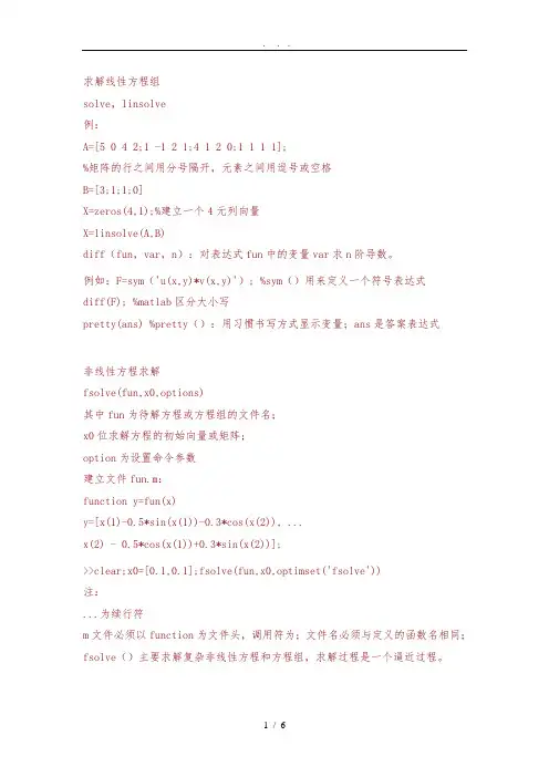
求解线性方程组solve,linsolve例:A=[5 0 4 2;1 -1 2 1;4 1 2 0;1 1 1 1];%矩阵的行之间用分号隔开,元素之间用逗号或空格B=[3;1;1;0]X=zeros(4,1);%建立一个4元列向量X=linsolve(A,B)diff(fun,var,n):对表达式fun中的变量var求n阶导数。
例如:F=sym('u(x,y)*v(x,y)'); %sym()用来定义一个符号表达式diff(F); %matlab区分大小写pretty(ans) %pretty():用习惯书写方式显示变量;ans是答案表达式非线性方程求解fsolve(fun,x0,options)其中fun为待解方程或方程组的文件名;x0位求解方程的初始向量或矩阵;option为设置命令参数建立文件fun.m:function y=fun(x)y=[x(1)-0.5*sin(x(1))-0.3*cos(x(2)), ...x(2) - 0.5*cos(x(1))+0.3*sin(x(2))];>>clear;x0=[0.1,0.1];fsolve(fun,x0,optimset('fsolve'))注:...为续行符m文件必须以function为文件头,调用符为;文件名必须与定义的函数名相同;fsolve()主要求解复杂非线性方程和方程组,求解过程是一个逼近过程。
Matlab求解线性方程组AX=B或XA=B在MATLAB中,求解线性方程组时,主要采用前面章节介绍的除法运算符“/”和“\”。
如:X=A\B表示求矩阵方程AX=B的解;X=B/A表示矩阵方程XA=B的解。
对方程组X=A\B,要求A和B用相同的行数,X和B有相同的列数,它的行数等于矩阵A的列数,方程X=B/A同理。
如果矩阵A不是方阵,其维数是m×n,则有:m=n 恰定方程,求解精确解;m>n 超定方程,寻求最小二乘解;m<n 不定方程,寻求基本解,其中至多有m个非零元素。
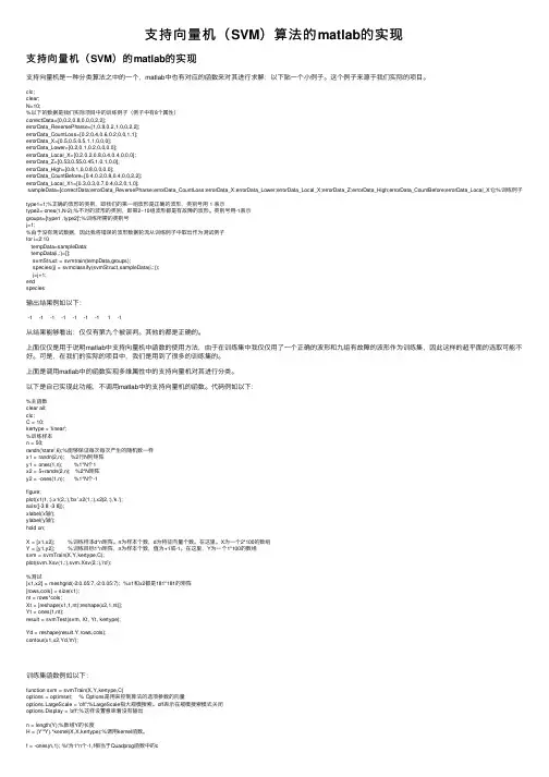
⽀持向量机(SVM)算法的matlab的实现⽀持向量机(SVM)的matlab的实现⽀持向量机是⼀种分类算法之中的⼀个,matlab中也有对应的函数来对其进⾏求解;以下贴⼀个⼩例⼦。
这个例⼦来源于我们实际的项⽬。
clc;clear;N=10;%以下的数据是我们实际项⽬中的训练例⼦(例⼦中有8个属性)correctData=[0,0.2,0.8,0,0,0,2,2];errorData_ReversePharse=[1,0.8,0.2,1,0,0,2,2];errorData_CountLoss=[0.2,0.4,0.6,0.2,0,0,1,1];errorData_X=[0.5,0.5,0.5,1,1,0,0,0];errorData_Lower=[0.2,0,1,0.2,0,0,0,0];errorData_Local_X=[0.2,0.2,0.8,0.4,0.4,0,0,0];errorData_Z=[0.53,0.55,0.45,1,0,1,0,0];errorData_High=[0.8,1,0,0.8,0,0,0,0];errorData_CountBefore=[0.4,0.2,0.8,0.4,0,0,2,2];errorData_Local_X1=[0.3,0.3,0.7,0.4,0.2,0,1,0];sampleData=[correctData;errorData_ReversePharse;errorData_CountLoss;errorData_X;errorData_Lower;errorData_Local_X;errorData_Z;errorData_High;errorData_CountBefore;errorData_Local_X1];%训练例⼦type1=1;%正确的波形的类别,即我们的第⼀组波形是正确的波形,类别号⽤ 1 表⽰type2=-ones(1,N-2);%不对的波形的类别,即第2~10组波形都是有故障的波形。
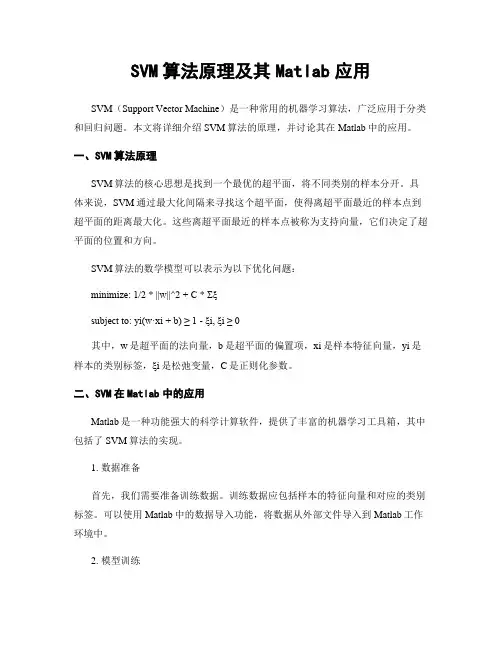
SVM算法原理及其Matlab应用SVM(Support Vector Machine)是一种常用的机器学习算法,广泛应用于分类和回归问题。
本文将详细介绍SVM算法的原理,并讨论其在Matlab中的应用。
一、SVM算法原理SVM算法的核心思想是找到一个最优的超平面,将不同类别的样本分开。
具体来说,SVM通过最大化间隔来寻找这个超平面,使得离超平面最近的样本点到超平面的距离最大化。
这些离超平面最近的样本点被称为支持向量,它们决定了超平面的位置和方向。
SVM算法的数学模型可以表示为以下优化问题:minimize: 1/2 * ||w||^2 + C * Σξsubject to: yi(w·xi + b) ≥ 1 - ξi, ξi ≥ 0其中,w是超平面的法向量,b是超平面的偏置项,xi是样本特征向量,yi是样本的类别标签,ξi是松弛变量,C是正则化参数。
二、SVM在Matlab中的应用Matlab是一种功能强大的科学计算软件,提供了丰富的机器学习工具箱,其中包括了SVM算法的实现。
1. 数据准备首先,我们需要准备训练数据。
训练数据应包括样本的特征向量和对应的类别标签。
可以使用Matlab中的数据导入功能,将数据从外部文件导入到Matlab工作环境中。
2. 模型训练接下来,我们可以使用Matlab中的svmtrain函数来训练SVM模型。
该函数的输入参数包括训练数据、正则化参数C和核函数类型等。
通过调整这些参数,可以得到不同的模型效果。
3. 模型评估训练完成后,我们可以使用svmclassify函数来对新的样本进行分类预测。
该函数的输入参数包括待分类的样本特征向量和训练得到的SVM模型。
函数将返回预测的类别标签。
4. 结果可视化为了更直观地观察分类结果,可以使用Matlab中的scatter函数将样本点绘制在二维平面上,并使用不同的颜色表示不同的类别。
5. 参数调优SVM算法中的正则化参数C和核函数类型等参数对模型的性能有重要影响。
在MATLAB中使用SVM进行模式识别的方法在MATLAB中,支持向量机(Support Vector Machine, SVM)是一种常用的模式识别方法。
SVM通过在特征空间中找到一个最优的超平面来分离不同的样本类别。
本文将介绍在MATLAB中使用SVM进行模式识别的一般步骤。
其次,进行特征选择与预处理。
在SVM中,特征选择是十分关键的一步。
合适的特征选择可以提取出最具有区分性的信息,从而提高SVM的分类效果。
特征预处理可以对样本数据进行归一化等,以确保特征具有相似的尺度。
然后,将数据集分为训练集和测试集。
可以使用MATLAB中的cvpartition函数来划分数据集。
一般来说,训练集用于训练SVM模型,测试集用于评估SVM的性能。
接下来,选择合适的核函数。
SVM利用核函数将数据映射到高维特征空间中,从而使得原本线性不可分的数据在新的特征空间中可分。
在MATLAB中,可以使用svmtrain函数的‘kernel_function’选项来选择不同的核函数,如线性核函数、多项式核函数、高斯核函数等。
然后,设置SVM的参数。
SVM有一些参数需要调整,如正则化参数C、软间隔的宽度等。
参数的选择会直接影响SVM的分类性能。
可以使用gridsearch函数或者手动调整参数来进行优化。
然后,用测试集测试SVM模型的性能。
使用svmclassify函数来对测试集中的样本进行分类。
svmclassify函数的输入是测试集特征向量和训练好的SVM模型。
最后,评估SVM的性能。
可以使用MATLAB中的confusionmat函数来计算分类结果的混淆矩阵。
根据混淆矩阵可以计算出准确率、召回率、F1分值等指标来评估SVM模型的性能。
除了上述步骤,还可以使用交叉验证、特征降维等方法进一步改进SVM的分类性能。
综上所述,通过以上步骤,在MATLAB中使用SVM进行模式识别的方法主要包括准备数据集,特征选择与预处理,数据集的划分,选择合适的核函数,设置SVM的参数,使用训练集训练SVM模型,用测试集测试SVM 模型的性能,评估SVM的性能等。
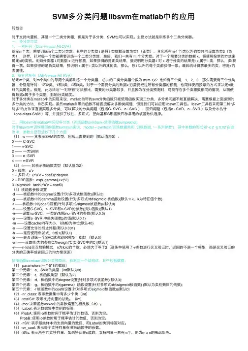
SVM多分类问题libsvm在matlab中的应⽤转载⾃对于⽀持向量机,其是⼀个⼆类分类器,但是对于多分类,SVM也可以实现。
主要⽅法就是训练多个⼆类分类器。
⼀、多分类⽅式1、⼀对所有(One-Versus-All OVA)给定m个类,需要训练m个⼆类分类器。
其中的分类器 i 是将 i 类数据设置为类1(正类),其它所有m-1个i类以外的类共同设置为类2(负类),这样,针对每⼀个类都需要训练⼀个⼆类分类器,最后,我们⼀共有 m 个分类器。
对于⼀个需要分类的数据 x,将使⽤投票的⽅式来确定x的类别。
⽐如分类器 i 对数据 x 进⾏预测,如果获得的是正类结果,就说明⽤分类器 i 对 x 进⾏分类的结果是: x 属于 i 类,那么,类i获得⼀票。
如果获得的是负类结果,那说明 x 属于 i 类以外的其他类,那么,除 i 以外的每个类都获得⼀票。
最后统计得票最多的类,将是x的类属性。
2、所有对所有(All-Versus-All AVA)给定m个类,对m个类中的每两个类都训练⼀个分类器,总共的⼆类分类器个数为 m(m-1)/2 .⽐如有三个类,1,2,3,那么需要有三个分类器,分别是针对:1和2类,1和3类,2和3类。
对于⼀个需要分类的数据x,它需要经过所有分类器的预测,也同样使⽤投票的⽅式来决定x最终的类属性。
但是,此⽅法与”⼀对所有”⽅法相⽐,需要的分类器较多,并且因为在分类预测时,可能存在多个类票数相同的情况,从⽽使得数据x属于多个类别,影响分类精度。
对于多分类在matlab中的实现来说,matlab⾃带的svm分类函数只能使⽤函数实现⼆分类,多分类问题不能直接解决,需要根据上⾯提到的多分类的⽅法,⾃⼰实现。
虽然matlab⾃带的函数不能直接解决多酚类问题,但是我们可以应⽤libsvm⼯具包。
libsvm⼯具包采⽤第⼆种“多对多”的⽅法来直接实现多分类,可以解决的分类问题(包括C- SVC、n - SVC )、回归问题(包括e - SVR、n - SVR )以及分布估计(one-class-SVM )等,并提供了线性、多项式、径向基和S形函数四种常⽤的核函数供选择。
MATLAB技术SVM算法实现引言:支持向量机(Support Vector Machine, SVM)是机器学习领域中一种常用的监督学习方法,广泛应用于分类和回归问题。
本文将介绍如何使用MATLAB技术实现SVM算法,包括数据预处理、特征选择、模型训练和性能评估等方面的内容。
一、数据预处理在使用SVM算法之前,我们需要先进行数据的预处理。
数据预处理是为了将原始数据转化为能够被SVM算法处理的形式,一般包括数据清洗、特征缩放和特征编码等步骤。
1. 数据清洗数据清洗是指对数据中的缺失值、异常值和噪声进行处理的过程。
在MATLAB中,可以使用诸如ismissing和fillmissing等函数来处理缺失值。
对于异常值和噪声的处理,可以使用统计学方法或者基于模型的方法。
2. 特征缩放特征缩放是指对特征值进行标准化处理的过程,使得各个特征值具有相同的量纲。
常用的特征缩放方法有均值归一化和方差归一化等。
在MATLAB中,可以使用zscore函数来进行特征缩放。
3. 特征编码特征编码是指将非数值型特征转化为数值型的过程,以便SVM算法能够对其进行处理。
常用的特征编码方法有独热编码和标签编码等。
在MATLAB中,可以使用诸如dummyvar和encode等函数来进行特征编码。
二、特征选择特征选择是指从原始特征中选择出最具有代表性的特征,以减少维度和提高模型性能。
在SVM算法中,选择合适的特征对分类效果非常关键。
1. 相关性分析通过分析特征与目标变量之间的相关性,可以选择与目标变量相关性较高的特征。
在MATLAB中,可以使用corrcoef函数计算特征之间的相关系数。
2. 特征重要性评估特征重要性评估可以通过各种特征选择方法来实现,如基于统计学方法的方差分析、基于模型的递归特征消除和基于树模型的特征重要性排序等。
在MATLAB 中,可以使用诸如anova1、rfimportance等函数进行特征重要性评估。
三、模型训练与评估在进行完数据预处理和特征选择之后,我们可以开始进行SVM模型的训练和评估了。
在当前数据挖掘和机器学习领域,最为热门的话题莫过于SVM和Boosting方法了。
只要是涉及到这两个主题,那么论文就会容易被杂志和会议接受了。
看来不管做什么,都讲究眼球效应啊。
搞研究其实也有点类似超级女声,呵呵。
以前我的论文中用的SVM Code都来自于台湾的林智仁教授的LibSVM。
真的是佩服有些大家,自己做出了重要的发现和成果,想到的不是把自己的成果保密起来(像C4.5一样),让自己独享自己的成果;而是让自己的成果最大程度的被人所利用,给后来的研究人员打下一个坚实的基础。
说实话,他的代码很好,用起来很方便,而且不同的语言版本实现都有,即使是对于初学者都很容易掌握。
不过用的久了,我就想自己也实现SVM,现在的数学计算工具太多了,而且功能齐全,用起来方便。
今天鼓捣了一会,终于用Matlab实现了第一个SVM。
虽然比较简单,但是包含了大多数SVM的必要步骤。
这个实现是线性可分支持向量分类机,不考虑非线性分类引入核函数的情况,也不考虑推广条件下引入Penalty Loss的情况。
问题描述:平面上有如下点A = [1 1.5;2 1.5;3 1.5;4 1.5;1 0.5;2 0.5;3 0.5;4 0.5]及其对应的标号flag = [1 1 1 1 -1 -1 -1 -1];用SVM方法构造一个决策函数实现正确分类。
如果我们在二维坐标上描点,就会发现这是个很简单的线性可分问题。
实现方法,用SVM 的对偶问题,转换为Matlab的有约束非线性规划问题。
构建m文件:function f = ffsvm(x)A = [1 1.5;2 1.5;3 1.5;4 1.5;1 0.5;2 0.5;3 0.5;4 0.5];flag = [1 1 1 1 -1 -1 -1 -1];for i=1:1:length(A)for j=1:1:length(A)normA(i,j) = A(i,:)*A(j,:)';normFlag(i,j) = flag(1,i)*flag(1,j);endendf = 0;for i=1:1:length(A)for j=1:1:length(A)f = f + 1/2*(normA(i,j)*x(i)*x(j)*normFlag(i,j));endf = f - x(i);end在命令窗口输入:Aeq = [1 1 1 1 -1 -1 -1 -1];beq = 0;lb = [ 0 0 0 0 0 0 0 0];调用MatLab内置优化函数fmincon;[x,favl,exitflag] = fmincon(@ffsvm,x0,[],[],Aeq,beq,lb,[])得到如下结果:Optimization terminated successfully:Magnitude of directional derivative in search directionless than 2*options.TolFun and maximum constraint violationis less than options.TolConActive Constraints:1x =0.5000 0.5000 0.5000 0.5000 0.5000 0.5000 0.5000 0.5000favl =-2.0000exitflag =1x的分量都不为0,说明这些点都是支持向量;计算w;w = [0 0];for i = 1:1:length(A)w = w + flag(i)*x(i)*A(i,:);end结果:w =[0,2];计算b;b = 0;for i=1:1:8b = b-flag(i)*x(i)*normA(i,1);endb = flag(1) + b;结果:b = -2;最终的决策函数为:f = sign([0, 2]*xT-2)可以验证,这个学习到的决策函数能够对这些平面上的点实现很好的分类;基本思路是这样的,如果要考虑引入核函数和Penalty Loss的情况,只需要修改优化函数和约束就可以实现。
matlab对三维数据的svm分类1.引言1.1 概述概述部分的内容可以包括对SVM分类算法和三维数据的概述。
在本文中,我们将探讨如何使用MATLAB来对三维数据进行支持向量机(SVM)分类。
SVM是一种常用的机器学习算法,可以用于二分类和多分类问题。
它通过寻找一个最优的超平面来将不同类别的数据分开,从而实现分类的目的。
三维数据是指具有三个特征向量的数据集。
这种类型的数据在许多领域中都很常见,例如医学图像处理、计算机视觉和工程分析等。
对于三维数据的分类,我们需要首先对数据进行表示和处理,以便用于SVM算法的输入。
本文的目的是介绍如何使用MATLAB对三维数据进行SVM分类。
我们将从SVM分类算法的基本原理开始,然后讨论如何表示和处理三维数据。
通过实验和结果分析,我们将评估SVM在三维数据分类中的性能,并总结结论。
通过本文的阅读,读者将能够了解SVM算法的基本原理、三维数据的表示和处理方法以及MATLAB在这方面的应用。
这将有助于读者在实际问题中应用SVM算法进行三维数据的分类分析。
1.2文章结构文章结构部分的内容可以按照以下方式编写:本文主要分为引言、正文和结论三个部分。
具体结构如下:2.正文正文部分主要包括两个主题:SVM分类算法和三维数据的表示和处理。
2.1 SVM分类算法在这个部分中,将介绍SVM分类算法的基本原理和步骤。
首先,会对支持向量机(SVM)进行简要的概述,包括其分类原理和优点。
然后,会详细介绍SVM分类算法的步骤,包括数据预处理、选择适当的核函数以及参数的调优等。
同时,还会讨论如何解决线性不可分数据和多类别分类的问题,并列举一些常用的SVM分类器的变形和扩展。
2.2 三维数据的表示和处理在这一部分中,将探讨如何在Matlab中表示和处理三维数据。
首先,会介绍三维数据的基本概念和特点,以及在实际应用中的重要性。
然后,会详细介绍在Matlab中如何使用矩阵和数组表示三维数据,并介绍一些常用的数据结构和操作。
matlab svm多分类算法-回复SVM (Support Vector Machine) 是一种常用的机器学习算法,在多分类问题中也可以被应用。
本文将以中括号内的内容为主题,一步一步回答关于Matlab 中SVM 多分类算法的问题。
一、什么是SVM 多分类算法?SVM 多分类算法是基于SVM 原理的一种分类器,它可以将输入的数据样本分为多个不同的类别。
SVM 多分类算法通过构建多个二分类问题的模型,来实现多分类任务。
简单来说,就是将多个二分类器结合起来,从而实现多分类的功能。
二、如何在Matlab 中使用SVM 多分类算法?在Matlab 中,可以使用内置的函数fitcecoc() 来实现SVM 多分类算法。
fitcecoc() 函数是一种通过Error-Correcting Output Codes (ECOC) 方法来训练多类SVM 的工具。
下面是一步一步的操作指南。
1. 准备数据:首先,我们需要准备用于训练和测试的数据。
这些数据应该包括输入特征和对应的类别标签。
可以使用Matlab 中的数据文件、数据集或自己创建的数据来进行训练和测试。
2. 设置参数:在使用SVM 多分类算法之前,需要设置一些参数。
例如,你可以选择SVM 的核函数类型、调整正则化参数等。
你可以在fitcecoc() 函数中根据实际情况进行相应的参数设置。
3. 划分数据集:为了评估模型的性能,我们需要将数据集划分为训练集和测试集。
可以使用crossvalind() 函数将数据集划分为K 个子集,其中K 为你选择的子集个数。
4. 训练模型:接下来,使用fitcecoc() 函数对训练集进行训练,得到一个多分类器。
5. 测试模型:然后,使用训练好的模型对测试集进行预测,并与真实的标签进行比较,以评估模型的性能。
可以使用predict() 函数来进行预测,并使用confusionmat() 函数生成混淆矩阵,以评估模型的分类准确度。
SVM算法原理及其Matlab应用支持向量机(Support Vector Machine,SVM)是一种常用的机器学习算法,它在分类和回归问题中都有广泛的应用。
本文将介绍SVM算法的原理,并探讨其在Matlab中的应用。
一、SVM算法原理SVM算法的核心思想是通过在特征空间中找到一个最优的超平面,将不同类别的样本分开。
其基本原理可以归结为以下几个关键步骤:1. 数据预处理:首先,需要对数据进行预处理,包括数据清洗、特征选择和特征缩放等。
这一步骤的目的是将原始数据转化为适合SVM算法处理的形式。
2. 特征映射:在某些情况下,数据在原始特征空间中无法线性可分。
为了解决这个问题,可以将数据映射到高维特征空间中,使得数据在新的特征空间中线性可分。
3. 构建超平面:在特征空间中,SVM算法通过构建一个超平面来将不同类别的样本分开。
这个超平面被定义为使得两个类别的间隔最大化的平面。
4. 支持向量:在构建超平面的过程中,SVM算法会选择一些样本点作为支持向量。
这些支持向量是距离超平面最近的样本点,它们对于分类结果的决策起到关键作用。
5. 分类决策:当新的样本点浮现时,SVM算法会根据其在特征空间中的位置,通过计算与超平面的距离来进行分类决策。
距离超平面较近的样本点很可能属于一个类别,而距离较远的样本点则很可能属于另一个类别。
二、SVM在Matlab中的应用Matlab作为一种强大的科学计算软件,提供了丰富的工具箱和函数来支持SVM算法的应用。
下面以一个简单的二分类问题为例,介绍SVM在Matlab中的应用过程。
首先,我们需要准备训练数据和测试数据。
在Matlab中,可以使用内置的数据集,或者自己准备数据。
然后,将数据进行预处理,包括特征选择和特征缩放等。
接下来,使用svmtrain函数来训练SVM模型。
该函数需要输入训练数据和相应的标签,以及一些参数,如核函数类型和惩罚参数等。
训练完成后,可以得到一个训练好的SVM模型。
在MATLAB中,最简单的SVM(支持向量机)例子可以通过以下步骤实现:1. 导入数据:首先,我们需要导入一些用于训练和测试的数据集。
这里我们使用MATLAB 内置的鸢尾花数据集。
```matlabload fisheriris; % 加载鸢尾花数据集X = meas; % 提取特征矩阵Y = species; % 提取标签向量```2. 划分训练集和测试集:我们将数据集划分为训练集和测试集,以便评估模型的性能。
```matlabcv = cvpartition(size(X,1),'HoldOut',0.5); % 划分训练集和测试集idx = cv.test; % 获取测试集的索引XTrain = X(~idx,:); % 提取训练集的特征矩阵YTrain = Y(~idx,:); % 提取训练集的标签向量XTest = X(idx,:); % 提取测试集的特征矩阵YTest = Y(idx,:); % 提取测试集的标签向量```3. 创建SVM模型:接下来,我们创建一个SVM模型,并设置相应的参数。
```matlabSVMModel = fitcsvm(XTrain,YTrain,'KernelFunction','linear'); % 创建线性核函数的SVM 模型```4. 预测和评估:最后,我们使用训练好的模型对测试集进行预测,并评估模型的性能。
```matlabYPred = predict(SVMModel,XTest); % 对测试集进行预测accuracy = sum(YPred == YTest)/length(YTest) * 100; % 计算准确率fprintf('Accuracy: %.2f%%', accuracy); % 输出准确率```这个例子展示了如何在MATLAB中使用最简单的SVM方法进行分类。
标题:MATLAB中SVM多分类算法的研究与应用摘要:支持向量机(Support Vector Machine,SVM)是一种常用的机器学习算法,在分类问题中表现出色。
然而,在面对多分类问题时,SVM的应用和优化仍然具有挑战性。
本文将对MATLAB中SVM 多分类算法的研究和应用进行深入探讨,分析其原理、优化方法以及实际应用。
通过本文的阅读,读者将能够全面了解MATLAB中SVM多分类算法的特点和应用技巧。
关键词:支持向量机;多分类算法;MATLAB;优化方法;应用技巧一、介绍支持向量机(SVM)是一种通过寻找最优超平面来进行分类的监督学习算法。
在二分类问题中,SVM表现出色,然而在面对多分类问题时,SVM的应用和性能仍然具有挑战性。
MATLAB作为一种强大的科学计算软件,具有丰富的机器学习工具包,其中包括了用于多分类问题的SVM算法。
本文将围绕MATLAB中SVM多分类算法的原理、优化方法以及实际应用展开讨论。
二、MATLAB中SVM多分类算法的原理1. SVM的基本原理SVM的基本原理是通过寻找一个最优的超平面来将不同类别的样本分开,使得两个类别的间隔最大化。
对于多分类问题,可以借助一对一(One-Versus-One)或一对其余(One-Versus-All)等方法来实现多个类别之间的分类。
MATLAB中的SVM多分类算法就是基于这样的原理进行实现的。
2. MATLAB中SVM多分类算法的实现MATLAB中提供了SVM多分类的函数,如fitcecoc和fitcsvm等,分别对应一对一和一对其余的多分类方法。
这些函数可以方便地对SVM进行训练和预测,同时还支持参数调优和模型评价等功能。
读者可以通过调用这些函数,快速实现SVM多分类算法的应用。
三、MATLAB中SVM多分类算法的优化方法1. 参数调优在使用SVM进行多分类时,参数的设置对算法的性能具有重要影响。
MATLAB中的SVM多分类算法支持对参数进行调优,如调整核函数类型、惩罚参数等,以提高算法的分类准确率和泛化能力。
Matlab_svmtranin_example1.Linear classification%Two Dimension Linear-SVM Problem,Two Class and Separable Situation%Method from Christopher J.C.Burges:%"A Tutorial on Support Vector Machines for Pattern Recognition",page9 %Optimizing||W||directly:%Objective:min"f(A)=||W||",p8/line26%Subject to:yi*(xi*W+b)-1>=0,function(12);clear all;close allclc;sp=[3,7;6,6;4,6;5,6.5]%positive sample pointsnsp=size(sp);sn=[1,2;3,5;7,3;3,4;6,2.7]%negative sample pointsnsn=size(sn)sd=[sp;sn]lsd=[true true true true false false false false false]Y=nominal(lsd)figure(1);subplot(1,2,1)plot(sp(1:nsp,1),sp(1:nsp,2),'m+');hold onplot(sn(1:nsn,1),sn(1:nsn,2),'c*');subplot(1,2,2)svmStruct=svmtrain(sd,Y,'showplot',true);2.NonLinear classification%Two Dimension quadratic-SVM Problem,Two Class and Separable Situation %Method from Christopher J.C.Burges:%"A Tutorial on Support Vector Machines for Pattern Recognition",page9 %Optimizing||W||directly:%Objective:min"f(A)=||W||",p8/line26%Subject to:yi*(xi*W+b)-1>=0,function(12);clear all;close allclc;sp=[3,7;6,6;4,6;5,6.5]%positive sample pointsnsp=size(sp);sn=[1,2;3,5;7,3;3,4;6,2.7;4,3;2,7]%negative sample pointsnsn=size(sn)sd=[sp;sn]lsd=[true true true true false false false false false false false]Y=nominal(lsd)figure(1);subplot(1,2,1)plot(sp(1:nsp,1),sp(1:nsp,2),'m+');hold onplot(sn(1:nsn,1),sn(1:nsn,2),'c*');subplot(1,2,2)%svmStruct=svmtrain(sd,Y,'Kernel_Function','linear','showplot',true);svmStruct=svmtrain(sd,Y,'Kernel_Function','quadratic','showplot',true);%use the trained svm(svmStruct)to classify the dataRD=svmclassify(svmStruct,sd,'showplot',true)%RD is the classification result vector3.Svmtrainsvmtrain Train a support vector machine classifierSVMSTRUCT=svmtrain(TRAINING,Y)trains a support vector machine(SVM) classifier on data taken from two groups.TRAINING is a numeric matrix of predictor data.Rows of TRAINING correspond to observations;columns correspond to features.Y is a column vector that contains the knownclass labels for TRAINING.Y is a grouping variable,i.e.,it can be a categorical,numeric,or logical vector;a cell vector of strings;or a character matrix with each row representing a class label(see help forgroupingvariable).Each element of Y specifies the group thecorresponding row of TRAINING belongs to.TRAINING and Y must have the same number of rows.SVMSTRUCT contains information about the trained classifier,including the support vectors,that is used by SVMCLASSIFY for classification.svmtrain treats NaNs,empty strings or'undefined' values as missing values and ignores the corresponding rows inTRAINING and Y.SVMSTRUCT=svmtrain(TRAINING,Y,'PARAM1',val1,'PARAM2',val2,...) specifies one or more of the following name/value pairs:Name Value'kernel_function'A string or a function handle specifying thekernel function used to represent the dotproduct in a new space.The value can be one ofthe following:'linear'-Linear kernel or dot product(default).In this case,svmtrainfinds the optimal separating planein the original space.'quadratic'-Quadratic kernel'polynomial'-Polynomial kernel with defaultorder3.To specify another order,use the'polyorder'argument.'rbf'-Gaussian Radial Basis Functionwith default scaling factor1.Tospecify another scaling factor,use the'rbf_sigma'argument.'mlp'-Multilayer Perceptron kernel(MLP)with default weight1and defaultbias-1.To specify another weightor bias,use the'mlp_params'argument.function-A kernel function specified using@(for example@KFUN),or ananonymous function.A kernelfunction must be of the formfunction K=KFUN(U,V)The returned value,K,is a matrixof size M-by-N,where M and N arethe number of rows in U and Vrespectively.'rbf_sigma'A positive number specifying the scaling factorin the Gaussian radial basis function kernel.Default is1.'polyorder'A positive integer specifying the order of thepolynomial kernel.Default is3.'mlp_params'A vector[P1P2]specifying the parameters of MLPkernel.The MLP kernel takes the form:K=tanh(P1*U*V'+P2),where P1>0and P2<0.Default is[1,-1].'method'A string specifying the method used to find theseparating hyperplane.Choices are:'SMO'-Sequential Minimal Optimization(SMO)method(default).It implements the L1soft-margin SVM classifier.'QP'-Quadratic programming(requires anOptimization Toolbox license).Itimplements the L2soft-margin SVMclassifier.Method'QP'doesn't scalewell for TRAINING with large number ofobservations.'LS'-Least-squares method.It implements theL2soft-margin SVM classifier.'options'Options structure created using either STATSET orOPTIMSET.*When you set'method'to'SMO'(default),create the options structure using STATSET.Applicable options:'Display'Level of display output.Choicesare'off'(the default),'iter',and'final'.Value'iter'reports every500iterations.'MaxIter'A positive integer specifying themaximum number of iterations allowed.Default is15000for method'SMO'.*When you set method to'QP',create theoptions structure using OPTIMSET.For detailsof applicable options choices,see QUADPROGoptions.SVM uses a convex quadratic program,so you can choose the'interior-point-convex'algorithm in QUADPROG.'tolkkt'A positive scalar that specifies the tolerancewith which the Karush-Kuhn-Tucker(KKT)conditionsare checked for method'SMO'.Default is1.0000e-003.'kktviolationlevel'A scalar specifying the fraction of observationsthat are allowed to violate the KKT conditions formethod'SMO'.Setting this value to be positivehelps the algorithm to converge faster if it isfluctuating near a good solution.Default is0.'kernelcachelimit'A positive scalar S specifying the size of thekernel matrix cache for method'SMO'.Thealgorithm keeps a matrix with up to S*Sdouble-precision numbers in memory.Default is5000.When the number of points in TRAININGexceeds S,the SMO method slows down.It'srecommended to set S as large as your systempermits.'boxconstraint'The box constraint C for the soft margin.C can bea positive numeric scalar or a vector of positivenumbers with the number of elements equal to thenumber of rows in TRAINING.Default is1.*If C is a scalar,it is automatically rescaledby N/(2*N1)for the observations of group one,and by N/(2*N2)for the observations of grouptwo,where N1is the number of observations ingroup one,N2is the number of observations ingroup two.The rescaling is done to take intoaccount unbalanced groups,i.e.,when N1and N2are different.*If C is a vector,then each element of Cspecifies the box constraint for thecorresponding observation.'autoscale'A logical value specifying whether or not toshift and scale the data points before training.When the value is true,the columns of TRAININGare shifted and scaled to have zero mean unitvariance.Default is true.'showplot'A logical value specifying whether or not to showa plot.When the value is true,svmtrain creates aplot of the grouped data and the separating linefor the classifier,when using data with2features(columns).Default is false. SVMSTRUCT is a structure having the following properties:SupportVectors Matrix of data points with each row correspondingto a support vector.Note:when'autoscale'is false,this fieldcontains original support vectors in TRAINING.When'autoscale'is true,this field containsshifted and scaled vectors from TRAINING.Alpha Vector of Lagrange multipliers for the supportvectors.The sign is positive for support vectorsbelonging to the first group and negative forsupport vectors belonging to the second group. Bias Intercept of the hyperplane that separatesthe two groups.Note:when'autoscale'is false,this fieldcorresponds to the original data points inTRAINING.When'autoscale'is true,this fieldcorresponds to shifted and scaled data points. KernelFunction The function handle of kernel function used. KernelFunctionArgs Cell array containing the additional argumentsfor the kernel function.GroupNames A column vector that contains the knownclass labels for TRAINING.Y is a groupingvariable(see help for groupingvariable). SupportVectorIndices A column vector indicating the indices of supportvectors.ScaleData This field contains information about auto-scale.When'autoscale'is false,it is empty.When'autoscale'is set to true,it is a structurecontaining two fields:shift-A row vector containing the negativeof the mean across all observationsin TRAINING.scaleFactor-A row vector whose value is1./STD(TRAINING).FigureHandles A vector of figure handles created by svmtrainwhen'showplot'argument is TRUE.Example:%Load the data and select features for classificationload fisheririsX=[meas(:,1),meas(:,2)];%Extract the Setosa classY=nominal(ismember(species,'setosa'));%Randomly partitions observations into a training set and a test %set using stratified holdoutP=cvpartition(Y,'Holdout',0.20);%Use a linear support vector machine classifiersvmStruct=svmtrain(X(P.training,:),Y(P.training),'showplot',true);C=svmclassify(svmStruct,X(P.test,:),'showplot',true);errRate=sum(Y(P.test)~=C)/P.TestSize%mis-classification rate conMat=confusionmat(Y(P.test),C)%the confusion matrix。
[matlab]支持向量机(SVM)用于分类的算法实现function [D, a_star] = SVM(train_features, train_targets, params, region)% Classify using (a very simple implementation of) the support vector machine algorithm%% Inputs:% features- Train features% targets - Train targets% params - [kernel, kernel parameter, solver type, Slack]% Kernel can be one of: Gauss, RBF (Same as Gauss), Poly, Sigmoid, or Linear % The kernel parameters are:% RBF kernel - Gaussian width (One parameter)% Poly kernel - Polynomial degree% Sigmoid - The slope and constant of the sigmoid (in the format [1 2], with no separating commas)% Linear - None needed% Solver type can be one of: Perceptron, Quadprog% region - Decision region vector: [-x x -y y number_of_points]%% Outputs% D - Decision sufrace% a - SVM coeficients%% Note: The number of support vectors found will usually be larger than is actually% needed because both solvers are approximate.[Dim, Nf] = size(train_features);Dim = Dim + 1;train_features(Dim,:) = ones(1,Nf);z = 2*(train_targets>0) - 1;%Get kernel parameters[kernel, ker_param, solver, slack] = process_params(params);%Transform the input featuresy = zeros(Nf);switch kernel,case {'Gauss','RBF'},for i = 1:Nf,y(:,i) = exp(-sum((train_features-train_features(:,i)*ones(1,Nf)).^2)'/(2*ker_param^2)); endcase {'Poly', 'Linear'}if strcmp(kernel, 'Linear')ker_param = 1;endfor i = 1:Nf,y(:,i) = (train_features'*train_features(:,i) + 1).^ker_param;endcase 'Sigmoid'if (length(ker_param) ~= 2)error('This kernel needs two parameters to operate!')endfor i = 1:Nf,y(:,i) = tanh(train_features'*train_features(:,i)*ker_param(1)+ker_param(2)); endotherwiseerror('Unknown kernel. Can be Gauss, Linear, Poly, or Sigmoid.')end%Find the SVM coefficientsswitch solvercase 'Quadprog'%Quadratic programmingif ~isfinite(slack)alpha_star = quadprog((z'*z).*(y'*y), -ones(1, Nf), [], [], z, 0, 0)';elsealpha_star = quadprog((z'*z).*(y'*y), -ones(1, Nf), [], [], z, 0, 0, slack)'; enda_star = (alpha_star.*z)*y';%Find the biasin = find((alpha_star > 0) & (alpha_star < slack));if isempty(in),bias = 0;elseB = z(in) - a_star * y(:,in);bias = mean(B(in));endcase 'Perceptron'max_iter = 1e5;iter = 0;rate = 0.01;xi = ones(1,Nf)/Nf*slack;if ~isfinite(slack),slack = 0;end%Find a start pointprocessed_y = [y; ones(1,Nf)] .* (ones(Nf+1,1)*z);a_star = mean(processed_y')';while ((sum(sign(a_star'*processed_y+xi)~=1)>0) & (iter < max_iter))iter = iter + 1;if (iter/5000 == floor(iter/5000)),disp(['Working on iteration number ' num2str(iter)])end%Find the worse classified sample (That farthest from the border)dist = a_star'*processed_y+xi;[m, indice] = min(dist);a_star = a_star + rate*processed_y(:,indice);%Calculate the new slack vectorxi(indice) = xi(indice) + rate;xi = xi / sum(xi) * slack;endif (iter == max_iter),disp(['Maximum iteration (' num2str(max_iter) ') reached']);elsedisp(['Converged after ' num2str(iter) ' iterations.'])endbias = 0;a_star = a_star(1:Nf)';case 'Lagrangian'%Lagrangian SVM (See Mangasarian & Musicant, Lagrangian Support Vector Machines) tol = 1e-5;max_iter = 1e5;nu = 1/Nf;iter = 0;D = diag(z);alpha = 1.9/nu;e = ones(Nf,1);I = speye(Nf);Q = I/nu + D*y'*D;P = inv(Q);u = P*e;oldu = u + 1;while ((iter<max_iter) & (sum(sum((oldu-u).^2)) > tol)), iter = iter + 1;if (iter/5000 == floor(iter/5000)),disp(['Working on iteration number ' num2str(iter)]) endoldu = u;f = Q*u-1-alpha*u;u = P*(1+(abs(f)+f)/2);enda_star = y*D*u(1:Nf);bias = -e'*D*u;otherwiseerror('Unknown solver. Can be either Quadprog or Perceptron') end%Find support verctorssv = find(abs(a_star) > 1e-10);Nsv = length(sv);if isempty(sv),error('No support vectors found');elsedisp(['Found ' num2str(Nsv) ' support vectors'])end%Marginb = 1/sqrt(sum(a_star.^2));disp(['The margin is ' num2str(b)])%Now build the decision regionN = region(5);xx = linspace (region(1),region(2),N);yy = linspace (region(3),region(4),N);D = zeros(N);for j = 1:N,y = zeros(N,1);for i = 1:Nsv,data = [xx(j)*ones(1,N); yy; ones(1,N)];switch kernel,case {'Gauss','RBF'},y = y + a_star(i) * exp(-sum((data-train_features(:,sv(i))*ones(1,N)).^2)'/(2*ker_param^2));case {'Poly', 'Linear'}y = y + a_star(i) * (data'*train_features(:,sv(i))+1).^ker_param;case 'Sigmoid'y = y + a_star(i) * tanh(data'*train_features(:,sv(i))*ker_param(1)+ker_param(2));endendD(:,j) = (y + bias);end。
MATLAB实例之对线性,非线性,超越方程的求解%对solve指令的使用%对线性,非线性,超越方程的求解%--------------------------------------------------------------------------%当方程组不存在符号解时,若又无其他自由参数,%则solve将给出数值解.%solve(S) 对一个方程默认变量求解%solve(S,v) 对一个方程指定变量v求解%solve(S1,S2,...,Sn) 对N个方程默认变量的求解%solve(S1,S2,...,Sn,v1,v2,...,vn) 对N个方程的v1,v2,...,vn变量求解%[x1,x2,...,xn]=solve(S1,S2,...,Sn) 对默认变量的求解并赋值%[x1,x2,...,xn]=solve(S1,S2,...,Sn,v1,v2,...,vn) 对指定变量的求解并赋值%-------------------------------------------------------------------------%例1%求解a*x^2+b*x+c=0,并求a=1,b=2,c=3时的数值解x=solve('a*x^2+b*x+c') %求符号解x=subs(x,'[a,b,c]',[1,2,3]) %代值,求数值解%例2%分别求方程sinx+btana=0当自变量为x和a时的解syms a b xf=sin(x)+b*tan(a);x=solve(f) %默认自变量为xa=solve(f,a) %指定自变量为a%例3%对方程组求解% x^2+x*y+y=a% x^2+b*x+c=0% 并求a=3,b=-4,c=3数值解s=solve('x^2+x*y+y=a','x^2+b*x+c=0') %输出构架数组x_sym=s.x %符号解y_sym=s.y %符号解x=subs(x_sym,'[a,b,c]',[3,-4,3]) %代入系数求数值解y=subs(y_sym,'[a,b,c]',[3,-4,3]) %求值%例4%求解方程组% y^2-z^2=x^2% y+z=a% x^2-b*x=c% 并求a=1,b=2,c=3时的x,y,z%[x,y,z]=solve('y^2-z^2-x^2','y+z-a','x^2-b*x-c') %求符号解a=1;b=2;c=3;xyz_value=eval([x,y,z]) %求数值解,注意,这里为两组解%%例5%求解方程组,指定自变量为a,b,c% y^2-z^2=x^2% y+z=a% x^2-b*x=c% 并求x=1,y=2,z=3时的a,b,c%syms a b c x y z;[a,b,c]=solve('y^2-z^2-x^2','y+z-a','x^2-b*x-c',a,b,c) %求符号解%解出来a b c为空的状态x=1;y=2;z=3; %已经没有意义了abc_value=eval([a,b,c]) %求数值解,注意,这里为两组解%%例6%重新构造方程组%求解方程组,指定自变量为a,b,c% a*x-b*y=c*z% y+z=a% x^2-b*x=c% 并求x=1,y=2,z=3时的a,b,c%syms a b c x y z;[a,b,c]=solve('a*x-b*y=c*z','y+z=a','x^2-b*x=c',a,b,c) %求符号解%x=1;y=2;z=3; %abc_value=eval([a,b,c]) %求数值解,注意,这里为两组解%%%本文来自CSDN博客,转载请标明出处:/hwb506/archive/2010/04/25/5523492.aspx。
Matlab_svmtranin_example1.Linear classification%Two Dimension Linear-SVM Problem, Two Class and Separable Situation%Method from Christopher J. C. Burges:%"A Tutorial on Support Vector Machines for Pattern Recognition", page 9 %Optimizing ||W|| directly:% Objective: min "f(A)=||W||" , p8/line26% Subject to: yi*(xi*W+b)-1>=0, function (12);clear all;close allclc;sp=[3,7; 6,6; 4,6;5,6.5] % positive sample pointsnsp=size(sp);sn=[1,2; 3,5;7,3;3,4;6,2.7] % negative sample pointsnsn=size(sn)sd=[sp;sn]lsd=[true true true true false false false false false]Y = nominal(lsd)figure(1);subplot(1,2,1)plot(sp(1:nsp,1),sp(1:nsp,2),'m+');hold onplot(sn(1:nsn,1),sn(1:nsn,2),'c*');subplot(1,2,2)svmStruct = svmtrain(sd,Y,'showplot',true);2.NonLinear classification%Two Dimension quadratic-SVM Problem, Two Class and Separable Situation%Method from Christopher J. C. Burges:%"A Tutorial on Support Vector Machines for Pattern Recognition", page 9 %Optimizing ||W|| directly:% Objective: min "f(A)=||W||" , p8/line26% Subject to: yi*(xi*W+b)-1>=0, function (12);clear all;close allclc;sp=[3,7; 6,6; 4,6; 5,6.5] % positive sample pointsnsp=size(sp);sn=[1,2; 3,5; 7,3; 3,4; 6,2.7; 4,3;2,7] % negative sample pointsnsn=size(sn)sd=[sp;sn]lsd=[true true true true false false false false false false false]Y = nominal(lsd)figure(1);subplot(1,2,1)plot(sp(1:nsp,1),sp(1:nsp,2),'m+');hold onplot(sn(1:nsn,1),sn(1:nsn,2),'c*');subplot(1,2,2)% svmStruct = svmtrain(sd,Y,'Kernel_Function','linear','showplot',true);svmStruct = svmtrain(sd,Y,'Kernel_Function','quadratic','showplot',true);% use the trained svm (svmStruct) to classify the dataRD=svmclassify(svmStruct,sd,'showplot',true)% RD is the classification result vector3.Svmtrainsvmtrain Train a support vector machine classifierSVMSTRUCT = svmtrain(TRAINING, Y) trains a support vector machine (SVM) classifier on data taken from two groups. TRAINING is a numeric matrix of predictor data. Rows of TRAINING correspond to observations; columns correspond to features. Y is a column vector that contains the knownclass labels for TRAINING. Y is a grouping variable, i.e., it can be a categorical, numeric, or logical vector; a cell vector of strings; or a character matrix with each row representing a class label (see help for groupingvariable). Each element of Y specifies the group thecorresponding row of TRAINING belongs to. TRAINING and Y must have the same number of rows. SVMSTRUCT contains information about the trained classifier, including the support vectors, that is used by SVMCLASSIFY for classification. svmtrain treats NaNs, empty strings or 'undefined' values as missing values and ignores the corresponding rows inTRAINING and Y.SVMSTRUCT = svmtrain(TRAINING, Y, 'PARAM1',val1, 'PARAM2',val2, ...) specifies one or more of the following name/value pairs:Name Value'kernel_function' A string or a function handle specifying thekernel function used to represent the dotproduct in a new space. The value can be one ofthe following:'linear' - Linear kernel or dot product(default). In this case, svmtrainfinds the optimal separating planein the original space.'quadratic' - Quadratic kernel'polynomial' - Polynomial kernel with defaultorder 3. To specify another order,use the 'polyorder' argument.'rbf' - Gaussian Radial Basis Functionwith default scaling factor 1. Tospecify another scaling factor,use the 'rbf_sigma' argument.'mlp' - Multilayer Perceptron kernel (MLP)with default weight 1 and defaultbias -1. To specify another weightor bias, use the 'mlp_params'argument.function - A kernel function specified using@(for example @KFUN), or ananonymous function. A kernelfunction must be of the formfunction K = KFUN(U, V)The returned value, K, is a matrixof size M-by-N, where M and N arethe number of rows in U and Vrespectively.'rbf_sigma' A positive number specifying the scaling factor in the Gaussian radial basis function kernel.Default is 1.'polyorder' A positive integer specifying the order of thepolynomial kernel. Default is 3.'mlp_params' A vector [P1 P2] specifying the parameters of MLP kernel. The MLP kernel takes the form:K = tanh(P1*U*V' + P2),where P1 > 0 and P2 < 0. Default is [1,-1].'method' A string specifying the method used to find theseparating hyperplane. Choices are:'SMO' - Sequential Minimal Optimization (SMO)method (default). It implements the L1soft-margin SVM classifier.'QP' - Quadratic programming (requires anOptimization Toolbox license). Itimplements the L2 soft-margin SVMclassifier. Method 'QP' doesn't scalewell for TRAINING with large number ofobservations.'LS' - Least-squares method. It implements theL2 soft-margin SVM classifier.'options' Options structure created using either STATSET or OPTIMSET.* When you set 'method' to 'SMO' (default),create the options structure using STATSET.Applicable options:'Display' Level of display output. Choicesare 'off' (the default), 'iter', and'final'. Value 'iter' reports every500 iterations.'MaxIter' A positive integer specifying themaximum number of iterations allowed.Default is 15000 for method 'SMO'.* When you set method to 'QP', create theoptions structure using OPTIMSET. For detailsof applicable options choices, see QUADPROGoptions. SVM uses a convex quadratic program,so you can choose the 'interior-point-convex'algorithm in QUADPROG.'tolkkt' A positive scalar that specifies the tolerancewith which the Karush-Kuhn-Tucker (KKT) conditions are checked for method 'SMO'. Default is1.0000e-003.'kktviolationlevel' A scalar specifying the fraction of observations that are allowed to violate the KKT conditions for method 'SMO'. Setting this value to be positivehelps the algorithm to converge faster if it isfluctuating near a good solution. Default is 0.'kernelcachelimit' A positive scalar S specifying the size of thekernel matrix cache for method 'SMO'. Thealgorithm keeps a matrix with up to S * Sdouble-precision numbers in memory. Default is5000. When the number of points in TRAININGexceeds S, the SMO method slows down. It'srecommended to set S as large as your systempermits.'boxconstraint' The box constraint C for the soft margin. C can bea positive numeric scalar or a vector of positivenumbers with the number of elements equal to thenumber of rows in TRAINING.Default is 1.* If C is a scalar, it is automatically rescaledby N/(2*N1) for the observations of group one,and by N/(2*N2) for the observations of grouptwo, where N1 is the number of observations ingroup one, N2 is the number of observations ingroup two. The rescaling is done to take intoaccount unbalanced groups, i.e., when N1 and N2are different.* If C is a vector, then each element of Cspecifies the box constraint for thecorresponding observation.'autoscale' A logical value specifying whether or not toshift and scale the data points before training.When the value is true, the columns of TRAININGare shifted and scaled to have zero mean unitvariance. Default is true.'showplot' A logical value specifying whether or not to show a plot. When the value is true, svmtrain creates a plot of the grouped data and the separating linefor the classifier, when using data with 2features (columns). Default is false.SVMSTRUCT is a structure having the following properties:SupportVectors Matrix of data points with each row corresponding to a support vector.Note: when 'autoscale' is false, this fieldcontains original support vectors in TRAINING.When 'autoscale' is true, this field containsshifted and scaled vectors from TRAINING.Alpha Vector of Lagrange multipliers for the supportvectors. The sign is positive for support vectorsbelonging to the first group and negative forsupport vectors belonging to the second group.Bias Intercept of the hyperplane that separatesthe two groups.Note: when 'autoscale' is false, this fieldcorresponds to the original data points inTRAINING. When 'autoscale' is true, this fieldcorresponds to shifted and scaled data points.KernelFunction The function handle of kernel function used.KernelFunctionArgs Cell array containing the additional argumentsfor the kernel function.GroupNames A column vector that contains the knownclass labels for TRAINING. Y is a groupingvariable (see help for groupingvariable).SupportVectorIndices A column vector indicating the indices of support vectors.ScaleData This field contains information about auto-scale. When 'autoscale' is false, it is empty. When'autoscale' is set to true, it is a structurecontaining two fields:shift - A row vector containing the negativeof the mean across all observationsin TRAINING.scaleFactor - A row vector whose value is1./STD(TRAINING).FigureHandles A vector of figure handles created by svmtrainwhen 'showplot' argument is TRUE.Example:% Load the data and select features for classificationload fisheririsX = [meas(:,1), meas(:,2)];% Extract the Setosa classY = nominal(ismember(species,'setosa'));% Randomly partitions observations into a training set and a test % set using stratified holdoutP = cvpartition(Y,'Holdout',0.20);% Use a linear support vector machine classifiersvmStruct =svmtrain(X(P.training,:),Y(P.training),'showplot',true);C = svmclassify(svmStruct,X(P.test,:),'showplot',true);errRate = sum(Y(P.test)~= C)/P.TestSize %mis-classification rate conMat = confusionmat(Y(P.test),C) % the confusion matrix。