rfc5439.An Analysis of Scaling Issues in MPLS-TE Core Networks
- 格式:pdf
- 大小:61.75 KB
- 文档页数:45

基于改进人工蜂群算法的边缘服务器部署策略
李波;袁也;侯鹏;丁洪伟
【期刊名称】《计算机应用与软件》
【年(卷),期】2024(41)5
【摘要】作为移动边缘计算架构部署的第一步,边缘服务器的部署是基础和关键,其部署位置与用户体验和系统性能密切相关,但是目前较少有研究关注该问题。
研究无线城域网中移动边缘计算环境下的边缘服务器部署问题,以最小化响应时间为目标,将边缘服务器部署问题定义为一个优化问题,并提出基于交叉的全局人工蜂群算法求解边缘服务器部署的最优解以降低系统的平均响应时间。
充分的实验结果表明,所提算法能够有效降低系统响应时间,算法性能优于其他代表性部署算法。
【总页数】8页(P218-225)
【作者】李波;袁也;侯鹏;丁洪伟
【作者单位】云南大学信息学院
【正文语种】中文
【中图分类】TP393
【相关文献】
1.基于四元数改进人工蜂群算法的彩色图像边缘检测
2.基于改进人工蜂群算法的多值属性系统故障诊断策略
3.基于改进人工蜂群算法的核电巡检机器人路径优化策略设计
4.基于改进人工蜂群算法的云资源调度策略
5.基于改进人工蜂群算法的自适应控制策略的设计及应用
因版权原因,仅展示原文概要,查看原文内容请购买。

第57卷第5期2017年5月电讯技术Telecommunication EngineeringV ol.57,N o.5May,2017d o i:10.3969/j.issn. 1001-893x.2017.05.001引用格式:潘乐炳,叶峻,曹满亮.战术认知无线电网络架构设计[J].电讯技术,2017,57(5):491-496.[PANLebing,YEJun,CAOManliang■ Architecture design of tactical cognitive radio networks[J]. Telecommunication Engineering,2017,57(5) ;491-496.]战术认知无线电网络架构设计+潘乐炳叫’2,叶峻\曹满亮1(1.中国电子科技集团公司第五十研究所,上海200331;2.中国电子科技集团公司数据链技术重点实验室,西安710068)摘要:认知无线电技术具有智能电磁频谱感知、干扰避免和动态频谱接入的能力,因此利用认知无线电技术可以提升战术网络的性能。
由于战术作战的复杂性,需要建立适用于战术任务的认知无线电架构。
首先分析了战术通信的特点和认知无线电技术在战术网络中的运用,以及目前国外战术认知无线网络的建设情况。
结合战术通信网络移动性高、电磁对抗复杂的特点,利用对抗环境下的战术网络结构和模型,提出了分层的战术认知无线电网络结构以及面向作战任务的网络管理方法,形 成拓扑结构分层次、管理运行分阶段的网络架构。
该网络架构均衡考虑了网络的灵活性和稳定性,适用于动态变化的战术网络,为认知无线电在战术通信中的技术应用和网络设计提供了参考。
关键词:认知无线电;战术通信;网络模型;网络管理架构中图分类号:TN92 文献标志码:A文章编号:1001-893X(2017)05-0491-06Architecture Design of Tactical Cognitive Radio NetworksPAN Lebing12,YE Jun1,CAO Manliang1(1. The 50th Research Institute of China Electronics Technology Group Corporation( C E T C),Shanghai 200331,China;2. CETC Key Laboratory of Data Link Technology,X i,an 710068,China)Abstract:Due to the ability of intelligent spectrum sensing,interference avoidance and dynamic spectrum access,cognitive radio technology can greatly enhance the performance of tactical networks.It is necessary to build a network architecture suitable for tactical task,which is complex in battlefield environment.F irst,the characteristics of tactical communication,the application of cognitive radio technology in tactical network and the foreign tactical cognitive radio networks are analyzed.According to the properties of high mobility and complex electromagnetic countermeasurement in the tactical communication network,a hierarchical model is proposed based on the competing tactical network structure,and a network management method is put forward to meet the tactical task.The network architecture with hierarchical topology and phased management is formed.The flexibility and stability of the network are both considered in this network architecture,therefore,it is suitable for dynamic tactical network and provides a reference for the application of cognitive radio in tactical communication.Key words:cognitive radio;tactical communication;network model;network management architecture1引言题越发突出,同时战术通信网络部署于动态变化的随着战术无线网络对大量数据交换需求的增长作战环境中,无线电干扰和波形参数突发改变时常 以及多传感器、多武器平台的接入,频谱资源匮乏问 发生,需要新的频谱共享机制来满足高频谱利用率 **收稿日期:2016-12-05;修回日期:2017-02-23 Received date :2016-12-05 ;Revised date :2017-02-23基金项目:中国电子科技集团公司数据链技术重点实验室开放基金(CLDL-20162410)**通信作者:forza@ aliyun. com Corresponding au thor : forza@ aliyun. com• 491•www . teleonline . cn电讯技术2017 年需求,同时还需考虑战场电磁频谱感知和无线干扰 避免。

基于规则的启发式搜索算法在飞机除冰调度中的应用的开题报告一、背景随着现代航空事业的飞速发展,飞机在起飞前必须进行除冰处理,以确保飞行安全。
而飞机除冰调度是指适时地协调地面雪、冰清除与飞机除冰,使得除冰操作在规定时间段内完成,从而避免飞机延误或事故,提高起飞成功率。
基于规则的启发式搜索算法被广泛应用于飞机除冰调度中,以优化除冰计划的制定。
二、研究意义在现代航空事业中,飞机除冰调度是个重要的问题,直接关系到飞行安全和经济效益。
而人工制定除冰计划需要考虑众多情况,而且效率低下,容易出现误差。
采用基于规则的启发式搜索算法,不仅能够自动化地制定除冰计划,而且能够在实际情况中动态地调整除冰方案,大大提高了效率和精度。
三、研究内容本论文将以飞机除冰调度为研究对象,重点研究基于规则的启发式搜索算法在这一领域中的应用。
具体来说,本论文将分析现有的除冰调度方法,总结其优缺点,并提出基于规则的启发式搜索算法在飞机除冰调度中的具体应用。
四、研究方法本论文将采用案例研究法,通过对已有案例的分析和总结,来研究基于规则的启发式搜索算法在飞机除冰调度中的应用。
具体来说,将选取多个不同规模和复杂度的除冰调度案例,分别采用基于规则的启发式搜索算法和现有方法进行比较,以验证该算法在飞机除冰调度中的适用性和优越性。
五、预期成果(1)总结现有飞机除冰调度方法,明确这些方法的优缺点;(2)提出基于规则的启发式搜索算法在飞机除冰调度中的具体应用;(3)对多个不同规模和复杂度的除冰调度案例进行基于规则的启发式搜索算法和现有方法的比较,证明该算法在飞机除冰调度中的适用性和优越性;(4)为飞机除冰调度的自动化和智能化提供参考。
六、研究计划本论文预计在一年内完成,具体研究计划如下:第1-2个月:梳理与归纳飞机除冰调度的现有方法,明确问题的研究范围和内容;第3-4个月:研究并总结基于规则的启发式搜索算法的原理和优势;第5-6个月:根据研究成果,提出基于规则的启发式搜索算法在飞机除冰调度中的具体应用;第7-8个月:选取多个不同规模和复杂度的除冰调度案例,分别采用基于规则的启发式搜索算法和现有方法进行比较;第9-10个月:分析和总结研究结果,撰写论文初稿;第11-12个月:修改论文,撰写最终论文,完成论文答辩。
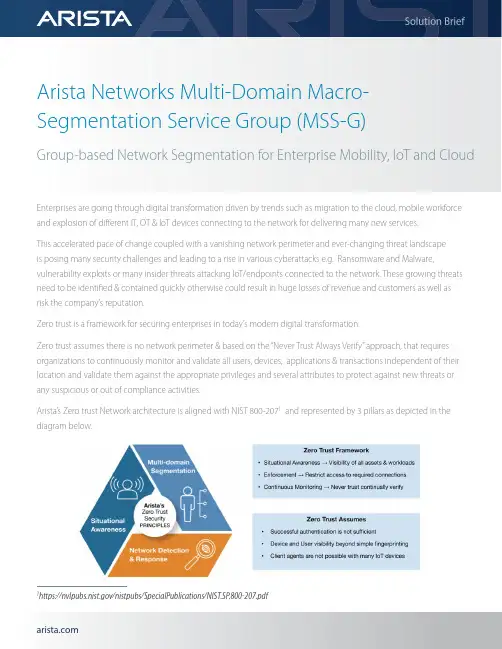
Arista Networks Multi-Domain Macro-Segmentation Service Group (MSS-G)Group-based Network Segmentation for Enterprise Mobility, IoT and CloudEnterprises are going through digital transformation driven by trends such as migration to the cloud, mobile workforce and explosion of different IT, OT & IoT devices connecting to the network for delivering many new services.This accelerated pace of change coupled with a vanishing network perimeter and ever-changing threat landscapeis posing many security challenges and leading to a rise in various cyberattacks e.g. Ransomware and Malware, vulnerability exploits or many insider threats attacking IoT/endpoints connected to the network. These growing threats need to be identified & contained quickly otherwise could result in huge losses of revenue and customers as well asrisk the company’s reputation.Zero trust is a framework for securing enterprises in today’s modern digital transformation.Zero trust assumes there is no network perimeter & based on the “Never Trust Always Verify” approach, that requires organizations to continuously monitor and validate all users, devices, applications & transactions independent of their location and validate them against the appropriate privileges and several attributes to protect against new threats or any suspicious or out of compliance activities.Arista’s Zero trust Network architecture is aligned with NIST 800-2071 and represented by 3 pillars as depicted in the diagram below.1https:///nistpubs/SpecialPublications/NIST.SP.800-207.pdfArista Zero Trust Networking Architecture is built on the same cloud principles which have become best practices across Datacenter, Campus and Cloud networks that uses Highly available leaf-spine network from Arista, Network Automation using Arista CloudVision, Telemetry for real-time visibility, monitoring and troubleshooting and Programmability & open APIs at every layer to allow faster integration with Arista ecosystem partners or any 3rd party system of choice.This paper covers Arista’s Group-based Multi Domain Segmentation, one of the pillars of Arista Zero Trust Architecture in more detail.While Network Segmentation is an effective way for reducing attack surface and limiting damage caused in one part of the network from proliferating to the entire network, traditional approaches based on network constructs (IP, subnet, VLANs..etc) or Access Control Lists (ACLs) are too rigid & operationally complex to manage, implementing those methods requires not only re-architecting the network but also managing thousands of ACLs manually on device-by-device basis.Enterprises require a segmentation approach that is flexible i.e. independent of the network constructs (IP, subnets, VLANs..Etc.), can scale and be simple to deploy considering both brownfield & greenfield environments.What is MSS-GroupMSS-Group or Group-Based Network Segmentation, part of Arista’s Zero Trust Networking Architecture, allows classification of endpoints into segments and security policy definition between those segments to allow or deny access. A given segment contains a set of endpoints that should have identical security properties within the network. Policies are then defined between segments rather than between endpoints and enforced on Arista EOS devices in hardware.MSS-Group Key Benefits• Flexible: Separates group policy from Network address boundaries• Simplified: No complex overlay protocols to configure & manage• Scalable: Efficient use of Data Plane Resources to overcome ACL Scale challenges• Standards-based Ethernet implementation: No-proprietary tags, can co-exist with 3rd party switches in network as long as enforcement is done on Arista Switches• Dynamic policy integration with ecosystem partners (e.g. Forescout)Use-casesEnterprise with Users, IT & OTCampuses and branches connecting different types of users (Employees, IT admin, Security-staff...etc), IT devices (Printers, Video Conferencing systems, IT Infrastructure e.g Switches/Routers, Servers...etc ) and OT devices (Security Cameras, Badge Readers, Building automation system, HVAC..etc) placed in different segments, irrespective of their location but depending on their security need and controlling access using segment policiesExamples:1. Allow access from Segment-1 (Employees) to Segment-11 (Printers, Video Conferencing)2. Allow access from Segment-2 (Security-staff) to Segment-12 (Security Camera, Badge Readers)3. Allow access from Segment-3 (IT admin) to Segment-13 ( IT Infrastructure)4. Deny access for everything else not matching above policies (Default-Policy)Compliance & RegulationPCI DSS (Payment Card Industry Data Security Standard) and HIPAA (Health Insurance Portability and Accountability Act) require protecting cardholder data and patient health records respectively. Network segmentation using MSS-G can help reduce the scope of compliance assessment by consolidating card holder data or patient health records into selective segments, controlling access thru MSS-G segment policies & thus minimizing the risk.Manufacturing Facility & Distribution CenterSegmenting resources for facilities, plants, production lines & corporate network in different groups and controlling access through MSS-G segment policies.Deployment OptionsCustomers have flexibility to use different options for deployment as below:• Arista CloudVision contains a built-in studio that allows users to define segments, assign devices to segments, create segment policies and apply the policy enforcement across the Network. CloudVision dashboard also provides an easy way to visualize and monitor any inter-segment forwarded and dropped traffic.• For dynamic policy, Forescout EyeSight and EyeSegment integrated with Arista CloudVision’s open APIs deliver a complete Zero Trust Solution by continuous discovery & monitoring of endpoints connected to switches, dynamically assign these endpoints to Groups, define segmentation policies and enforce these policy across the network through Arista CloudVision.• Customers who would prefer their own policy management solution can connect to CloudVision through open APIs or even manage switches directly using Arista EOS CLI or EAPI.Santa Clara—Corporate Headquarters 5453 Great America Parkway,Santa Clara, CA 95054Phone: +1-408-547-5500Fax: +1-408-538-8920Email:***************Ireland—International Headquarters3130 Atlantic AvenueWestpark Business CampusShannon, Co. ClareIrelandVancouver—R&D Office9200 Glenlyon Pkwy, Unit 300Burnaby, British ColumbiaCanada V5J 5J8San Francisco—R&D and Sales Office 1390Market Street, Suite 800San Francisco, CA 94102India—R&D OfficeGlobal Tech Park, Tower A, 11th FloorMarathahalli Outer Ring RoadDevarabeesanahalli Village, Varthur HobliBangalore, India 560103Singapore—APAC Administrative Office9 Temasek Boulevard#29-01, Suntec Tower TwoSingapore 038989Nashua—R&D Office10 Tara BoulevardNashua, NH 03062Copyright © 2022 Arista Networks, Inc. All rights reserved. CloudVision, and EOS are registered trademarks and Arista Networks is a trademark of Arista Networks, Inc. All other company names are trademarks of their respective holders. Information in this document is subject to change without notice. Certain features may not yet be available. Arista Networks, Inc. assumes no responsibility for any errors that may appear in this document. June 21, 2022ConclusionMSS-G or Group-Based Network Segmentation, part of Arista’s Zero Trust Networking Architecture is a simple, non-proprietary, flexible & scalable security solution for segmenting users, IT, OT and IoT devices. MSS-G can effectively reduce attack surface, limit the scope of compliance & regulation assessment & thus overall reduce the risk for organizations.Reference:https:///assets/data/pdf/Whitepapers/Arista-Zero-Trust-Security-for-Cloud-Networking.pdfhttps:///assets/data/pdf/Whitepapers/Network-Automation-CloudVision-Studios-WP.pdf。

万方数据万方数据万方数据万方数据万方数据万方数据万方数据京津冀城市群的功能联系及其复杂网络演化作者:赵渺希, 魏冀明, 吴康, ZHAO Miaoxi, WEI Jiming, WU Kang作者单位:赵渺希,ZHAO Miaoxi(华南理工大学建筑学院/亚热带建筑科学国家重点实验室), 魏冀明,WEI Jiming(华南理工大学建筑学院), 吴康,WU Kang(首都经济贸易大学城市经济与公共管理学院)刊名:城市规划学刊英文刊名:Urban Planning Forum年,卷(期):2014(1)1.ALDERSON A;BECKFIELD J Power and position in the world city system 20042.ALDERSON A S;BECKFIELDJ;SPRAGUEJONES J Intercity relations and globalisation:the evolution of the global urban hierarchy1981-2007 2010(9)3.BARAB(A)SI A;ALBERT R Emergence of scaling in random networks[外文期刊] 1999(5439)4.BARRAT A;BARTH(E)LEMY M;Vespignani A Weighted evolving networks:coupling topology and weight dynamics 2004(22)5.BATTEN D F Network cities:creative urban agglomerations for the 21st Century 1995(2)6.BATTY M Polynucleated urban Landscapes 2001(4)7.BOCCALETTI S;LATORA V;MORENO Y Complex networks:structure and dynamics 20068.BURGER M;MEIJERS E Form follows function? linking morphological and functional polycentricity 2012(5)9.BURGER M;KNAAP B;WALL R Polycentricity and the multiplexity of urban networks 201310.CAIMCROSS F The death of distance:how the communications revolution is changing our lives 200111.CAPELLO R;CAMAGNI R Beyond optimal city size:an evaluation of alternative urban growth patterns 200012.CASTELLS M The rise of the network society 199613.DERUDDER B;LIU XJ Analyzing urban networks through the lens of corporate networks:a ctitical review 201314.DERUDDER B;TIMBERLAKE M;WITLOX F Introduction:mapping changes in urban systems 2010(9)15.TAYLOR D B;P J;N1 P Pathways of change:shifting connectivities in the world city network,2000-08 2010(9)16.GREEN N Functional polycentricity:a formal definition in terms of social network analysis 2007(11)17.HALL P;PAIN K The polycentric metropolis:learning from mega-city regions in europe 200618.胡祖光基尼系数理论最佳值及其简易计算公式研究[期刊论文]-{H}经济研究 2004(9)19.JACOBS W;KOSTER H;HALL P The location and global network structure of maritime advanced producer services 2011(13)20.KLOOSTERMAN R;MUSTERD S The polycentric urban region:towards a research agenda 2001TORA V;MARCHIORI M Efficient behavior of small-world networks 2001(19)22.LIMTANAKOOL N;DIJST M;SCHWANEN T A theoretical framework and methodology for characterising national urban systems on the basis of flows of people:empirical evidencefor france and germany 2007(11)23.LIU X J;DERUDDER B Two-mode networks and the interlocking world city network model:A reply to Neal 2012(2)24.罗震东;何鹤鸣;耿磊基于客运交通流的长江三角洲功能多中心结构研究[期刊论文]-{H}城市规划学刊 2011(2)25.MASSEY D B Spatial divisions of labor:social structures and the geography of production 199526.MAHUTGA M C;MA X Economic globalisation and the structure of the world city system:the case of airline passenger data 2010(9)27.MATTHIESSEN C W;SCHWARZ A W;FIND S World cities of scientific knowledge:systems,networks and potential dynamics.an analysis based on bibliometric indicators' 2010(9)28.MEIJERS E J Synergy in polycentric urban regions:complementarity,organizing capacity and critical mass 200729.MEIJERS E J Measuring Polycentricity and its premises 2008(9)30.GASTNER M T;NEWMAN M The spatial structure of networks 200631.NEAL Z From central places to network bases:a transition in the U.S.Urban Hierarchy,1900-2000 2011(1)32.Neal Z Structural determinism in the interlocking world city network 2012(2)33.NEWMAN M Assortative mixing in networks 2002(20)34.PARR J The polycentric urban region:a closer inspection 2004(3)35.SASSEN S The global city:new york,London,tokyo 200136.SCOTT A J;STORPER M Regions,globalization,development 2003(6-7)37.唐子来;赵渺希经济全球化视角下长三角区域的城市体系演化:关联网络和价值区段的分析方法[期刊论文]-{H}城市规划学刊2010(1)38.TAYLOR P Specification of the world city network 200139.TOFFLER A The third wave 198040.WATTS D;STROGATZ S Collective dynamics of 'small-world' networks 1998(6684)41.吴良镛京津冀北城乡空间发展规划研究Ⅱ 2000(12)42.赵渺希;朵朵巨型城市区域的复杂网络特征 2013(6)引用本文格式:赵渺希.魏冀明.吴康.ZHAO Miaoxi.WEI Jiming.WU Kang京津冀城市群的功能联系及其复杂网络演化[期刊论文]-城市规划学刊 2014(1)。

Network Working Group M. Baugher Request for Comments: 3547 B. Weis Category: Standards Track Cisco T. Hardjono Verisign H. Harney Sparta July 2003 The Group Domain of InterpretationStatus of this MemoThis document specifies an Internet standards track protocol for the Internet community, and requests discussion and suggestions forimprovements. Please refer to the current edition of the "InternetOfficial Protocol Standards" (STD 1) for the standardization stateand status of this protocol. Distribution of this memo is unlimited.Copyright NoticeCopyright (C) The Internet Society (2003). All Rights Reserved.AbstractThis document presents an ISAMKP Domain of Interpretation (DOI) forgroup key management to support secure group communications. TheGDOI manages group security associations, which are used by IPSEC and potentially other data security protocols running at the IP orapplication layers. These security associations protect one or more key-encrypting keys, traffic-encrypting keys, or data shared by group members.Table of Contents1. Introduction . . . . . . . . . . . . . . . . . . . . . . . . . 3 1.1. GDOI Applications. . . . . . . . . . . . . . . . . . . . 51.2. Extending GDOI . . . . . . . . . . . . . . . . . . . . . 52. GDOI Phase 1 protocol. . . . . . . . . . . . . . . . . . . . . 6 2.1. ISAKMP Phase 1 protocol. . . . . . . . . . . . . . . . . 6 2.1.1. DOI value. . . . . . . . . . . . . . . . . . . . 62.1.2. UDP port . . . . . . . . . . . . . . . . . . . . 63. GROUPKEY-PULL Exchange . . . . . . . . . . . . . . . . . . . . 6 3.1. Authorization. . . . . . . . . . . . . . . . . . . . . . 7 3.2. Messages . . . . . . . . . . . . . . . . . . . . . . . . 7 3.2.1. Perfect Forward Secrecy. . . . . . . . . . . . . 9 3.2.2. ISAKMP Header Initialization . . . . . . . . . . 9 Baugher, et. al. Standards Track [Page 1]3.3. Initiator Operations . . . . . . . . . . . . . . . . . . 103.4. Receiver Operations. . . . . . . . . . . . . . . . . . . 114. GROUPKEY-PUSH Message. . . . . . . . . . . . . . . . . . . . . 11 4.1. Perfect Forward Secrecy (PFS). . . . . . . . . . . . . . 12 4.2. Forward and Backward Access Control. . . . . . . . . . . 12 4.2.1. Forward Access Control Requirements. . . . . . . 13 4.3. Delegation of Key Management . . . . . . . . . . . . . . 14 4.4. Use of signature keys. . . . . . . . . . . . . . . . . . 14 4.5. ISAKMP Header Initialization . . . . . . . . . . . . . . 14 4.6. Deletion of SAs. . . . . . . . . . . . . . . . . . . . . 14 4.7. GCKS Operations. . . . . . . . . . . . . . . . . . . . . 154.8. Group Member Operations. . . . . . . . . . . . . . . . . 165. Payloads and Defined Values. . . . . . . . . . . . . . . . . . 16 5.1. Identification Payload . . . . . . . . . . . . . . . . . 17 5.1.1. Identification Type Values . . . . . . . . . . . 18 5.2. Security Association Payload . . . . . . . . . . . . . . 18 5.2.1. Payloads following the SA payload. . . . . . . . 19 5.3. SA KEK payload . . . . . . . . . . . . . . . . . . . . . 19 5.3.1. KEK Attributes . . . . . . . . . . . . . . . . . 22 5.3.2. KEK_MANAGEMENT_ALGORITHM . . . . . . . . . . . . 22 5.3.3. KEK_ALGORITHM. . . . . . . . . . . . . . . . . . 23 5.3.4. KEK_KEY_LENGTH . . . . . . . . . . . . . . . . . 23 5.3.5. KEK_KEY_LIFETIME . . . . . . . . . . . . . . . . 24 5.3.6. SIG_HASH_ALGORITHM . . . . . . . . . . . . . . . 24 5.3.7. SIG_ALGORITHM. . . . . . . . . . . . . . . . . . 24 5.3.8. SIG_KEY_LENGTH . . . . . . . . . . . . . . . . . 25 5.3.9. KE_OAKLEY_GROUP. . . . . . . . . . . . . . . . . 25 5.4. SA TEK Payload . . . . . . . . . . . . . . . . . . . . . 25 5.4.1. PROTO_IPSEC_ESP. . . . . . . . . . . . . . . . . 26 5.4.2. Other Security Protocols . . . . . . . . . . . . 28 5.5. Key Download Payload . . . . . . . . . . . . . . . . . . 28 5.5.1. TEK Download Type. . . . . . . . . . . . . . . . 30 5.5.2. KEK Download Type. . . . . . . . . . . . . . . . 31 5.5.3. LKH Download Type. . . . . . . . . . . . . . . . 32 5.6. Sequence Number Payload. . . . . . . . . . . . . . . . . 35 5.7. Proof of Possession. . . . . . . . . . . . . . . . . . . 365.8. Nonce. . . . . . . . . . . . . . . . . . . . . . . . . . 366. Security Considerations. . . . . . . . . . . . . . . . . . . . 36 6.1. ISAKMP Phase 1 . . . . . . . . . . . . . . . . . . . . . 37 6.1.1. Authentication . . . . . . . . . . . . . . . . . 37 6.1.2. Confidentiality. . . . . . . . . . . . . . . . . 37 6.1.3. Man-in-the-Middle Attack Protection. . . . . . . 38 6.1.4. Replay/Reflection Attack Protection. . . . . . . 38 6.1.5. Denial of Service Protection . . . . . . . . . . 38 6.2. GROUPKEY-PULL Exchange . . . . . . . . . . . . . . . . . 38 6.2.1. Authentication . . . . . . . . . . . . . . . . . 38 6.2.2. Confidentiality. . . . . . . . . . . . . . . . . 39 6.2.3. Man-in-the-Middle Attack Protection. . . . . . . 39 Baugher, et. al. Standards Track [Page 2]6.2.4. Replay/Reflection Attack Protection. . . . . . . 39 6.2.5. Denial of Service Protection . . . . . . . . . . 39 6.2.6. Authorization. . . . . . . . . . . . . . . . . . 40 6.3. GROUPKEY-PUSH Exchange . . . . . . . . . . . . . . . . . 40 6.3.1. Authentication . . . . . . . . . . . . . . . . . 40 6.3.2. Confidentiality. . . . . . . . . . . . . . . . . 40 6.3.3. Man-in-the-Middle Attack Protection. . . . . . . 40 6.3.4. Replay/Reflection Attack Protection. . . . . . . 40 6.3.5. Denial of Service Protection . . . . . . . . . . 416.3.6. Forward Access Control . . . . . . . . . . . . . 417. IANA Considerations. . . . . . . . . . . . . . . . . . . . . . 41 7.1. ISAKMP DOI . . . . . . . . . . . . . . . . . . . . . . . 41 7.2. Payload Types. . . . . . . . . . . . . . . . . . . . . . 42 7.3. New Name spaces. . . . . . . . . . . . . . . . . . . . . 427.4. UDP Port . . . . . . . . . . . . . . . . . . . . . . . . 428. Intellectual Property Rights Statement . . . . . . . . . . . . 429. Acknowledgements . . . . . . . . . . . . . . . . . . . . . . . 4310. References . . . . . . . . . . . . . . . . . . . . . . . . . . 43 10.1. Normative References . . . . . . . . . . . . . . . . . . 43 10.2. Informative References . . . . . . . . . . . . . . . . . 44 Appendix A: Alternate GDOI Phase 1 protocols . . . . . . . . . . . 46 A.1. IKEv2 Phase 1 protocol . . . . . . . . . . . . . . . . . 46 A.2. KINK Protocol. . . . . . . . . . . . . . . . . . . . . . 46 Authors’ Addresses . . . . . . . . . . . . . . . . . . . . . . . . 47 Full Copyright Statement . . . . . . . . . . . . . . . . . . . . . 48 1. IntroductionThis document presents an ISAMKP Domain of Interpretation (DOI) forgroup key management called the "Group Domain of Interpretation"(GDOI). In this group key management model, the GDOI protocol is run between a group member and a "group controller/key server" (GCKS),which establishes security associations [Section 4.6.2 RFC2401] among authorized group members. ISAKMP defines two "phases" of negotiation [p.16 RFC2408]. The GDOI MUST be protected by a Phase 1 securityassociation. This document incorporates the Phase 1 securityassociation (SA) definition from the Internet DOI [RFC2407, RFC2409]. Other possible Phase 1 security association types are noted inAppendix A. The Phase 2 exchange is defined in this document, andproposes new payloads and exchanges according to the ISAKMP standard [p. 14 RFC2408].There are six new payloads:1) GDOI SA2) SA KEK (SAK) which follows the SA payload3) SA TEK (SAT) which follows the SA payloadBaugher, et. al. Standards Track [Page 3]4) Key Download Array (KD)5) Sequence number (SEQ)6) Proof of Possession (POP)There are two new exchanges.1) A Phase 2 exchange creates Re-key and Data-Security Protocol SAs. The new Phase 2 exchange, called "GROUPKEY-PULL," downloads keys for a group’s "Re-key" SA and/or "Data-security" SA. The Re-key SAincludes a key encrypting key, or KEK, common to the group; aData-security SA includes a data encryption key, or TEK, used by adata-security protocol to encrypt or decrypt data traffic [Section2.1 RFC2407]. The SA for the KEK or TEK includes authenticationkeys, encryption keys, cryptographic policy, and attributes. TheGROUPKEY-PULL exchange uses "pull" behavior since the memberinitiates the retrieval of these SAs from a GCKS.2) A datagram subsequently establishes additional Rekey and/orData-Security Protocol SAs.The GROUPKEY-PUSH datagram is "pushed" from the GCKS to the membersto create or update a Re-key or Data-security SA. A Re-key SAprotects GROUPKEY-PUSH messages. Thus, a GROUPKEY-PULL is necessary to establish at least one Re-key SA in order to protect subsequentGROUPKEY-PUSH messages. The GCKS encrypts the GROUPKEY-PUSH message using the KEK Re-key SA. GDOI accommodates the use of arrays of KEKs for group key management algorithms using the Logical Key Hierarchy(LKH) algorithm to efficiently add and remove group members[RFC2627]. Implementation of the LKH algorithm is OPTIONAL.Although the GROUPKEY-PUSH specified by this document can be used to refresh a Re-key SA, the most common use of GROUPKEY-PUSH is toestablish a Data-security SA for a data security protocol. GDOI can accommodate future extensions to support a variety of data securityprotocols. This document only specifies data-security SAs for onesecurity protocol, IPsec ESP. A separate RFC will specify supportfor other data security protocols such as a future secure Real-timeTransport Protocol. A security protocol uses the TEK and "owns" the data-security SA in the same way that IPsec ESP uses the IKE Phase 2 keys and owns the Phase 2 SA; for GDOI, IPsec ESP uses the TEK.Thus, GDOI is a group security association management protocol: AllGDOI messages are used to create, maintain, or delete securityassociations for a group. As described above, these securityassociations protect one or more key-encrypting keys,traffic-encrypting keys, or data shared by group members formulticast and groups security applications.Baugher, et. al. Standards Track [Page 4]The keywords MUST, MUST NOT, REQUIRED, SHALL, SHALL NOT, SHOULD,SHOULD NOT, RECOMMENDED, MAY, and OPTIONAL, when they appear in this document, are to be interpreted as described in BCP 14, RFC 2119[RFC2119].1.1. GDOI ApplicationsSecure multicast applications include video broadcast and multicastfile transfer. In a business environment, many of these applications require network security and may use IPsec ESP to secure their datatraffic. Section 5.4.1 specifies how GDOI carries the needed SAparameters for ESP. In this way, GDOI supports multicast ESP withgroup authentication of ESP packets using the shared, group key(authentication of unique sources of ESP packets is not possible).GDOI can also secure group applications that do not use multicasttransport such as video-on-demand. For example, the GROUPKEY-PUSHmessage may establish a pair-wise IPsec ESP SA for a member of asubscription group without the need for key management exchanges and costly asymmetric cryptography.1.2. Extending GDOINot all secure multicast or multimedia applications can use IPsecESP. Many Real Time Transport Protocol applications, for example,require security above the IP layer to preserve RTP headercompression efficiencies and transport-independence [RFC3550]. Afuture RTP security protocol may benefit from using GDOI to establish group SAs.In order to add a new data security protocol, a new RFC MUST specify the data-security SA parameters conveyed by GDOI for that securityprotocol; these parameters are listed in section 5.4.2 of thisdocument.Data security protocol SAs MUST protect group traffic. GDOI provides no restriction on whether that group traffic is transmitted asunicast or multicast packets. However, GDOI MUST NOT be used as akey management mechanism by a data security protocol when the packets protected by the data-security SA are intended to be private andnever become part of group communications.Baugher, et. al. Standards Track [Page 5]2. GDOI Phase 1 protocolGDOI is a "phase 2" protocol which MUST be protected by a "phase 1"protocol. The "phase 1" protocol can be any protocol which provides for the following protections:o Peer Authenticationo Confidentialityo Message IntegrityThe following sections describe one such "phase 1" protocol. Otherprotocols which may be potential "phase 1" protocols are described in Appendix A. However, the use of the protocols listed there are notconsidered part of this document.2.1. ISAKMP Phase 1 protocolThis document defines how the ISAKMP phase 1 exchanges as defined in [RFC2409] can be used a "phase 1" protocol for GDOI. The followingsections define characteristics of the ISAKMP phase 1 protocols that are unique for these exchanges when used for GDOI.Section 6.1 describes how the ISAKMP Phase 1 protocols meet therequirements of a GDOI "phase 1" protocol.2.1.1. DOI valueThe Phase 1 SA payload has a DOI value. That value MUST be the GDOI DOI value as defined later in this document.2.1.2. UDP portGDOI MUST NOT run on port 500 (the port commonly used for IKE). IANA has assigned port 848 for the use of GDOI.3. GROUPKEY-PULL ExchangeThe goal of the GROUPKEY-PULL exchange is to establish a Re-keyand/or Data-security SAs at the member for a particular group. APhase 1 SA protects the GROUPKEY-PULL; there MAY be multipleGROUPKEY-PULL exchanges for a given Phase 1 SA. The GROUPKEY-PULLexchange downloads the data security keys (TEKs) and/or group keyencrypting key (KEK) or KEK array under the protection of the Phase 1 SA.Baugher, et. al. Standards Track [Page 6]3.1. AuthorizationThere are two alternative means for authorizing the GROUPKEY-PULLmessage. First, the Phase 1 identity can be used to authorize thePhase 2 (GROUPKEY-PULL) request for a group key. Second, a newidentity can be passed in the GROUPKEY-PULL request. The newidentity could be specific to the group and use a certificate that is signed by the group owner to identify the holder as an authorizedgroup member. The Proof-of-Possession payload validates that theholder possesses the secret key associated with the Phase 2 identity.3.2. MessagesThe GROUPKEY-PULL is a Phase 2 exchange. Phase 1 computes SKEYID_awhich is the "key" in the keyed hash used in the GROUPKEY-PULL HASHpayloads. When using the Phase 1 defined in this document, SKEYID_a is derived according to [RFC2409]. As with the IKE HASH payloadgeneration [RFC 2409 section 5.5], each GROUPKEY-PULL message hashes a uniquely defined set of values. Nonces permute the HASH andprovide some protection against replay attacks. Replay protection is important to protect the GCKS from attacks that a key managementserver will attract.The GROUPKEY-PULL uses nonces to guarantee "liveliness", or againstreplay of a recent GROUPKEY-PULL message. The replay attack is only useful in the context of the current Phase 1. If a GROUPKEY-PULLmessage is replayed based on a previous Phase 1, the HASH calculation will fail due to a wrong SKEYID_a. The message will fail processing before the nonce is ever evaluated. In order for either peer to get the benefit of the replay protection, it must postpone as muchprocessing as possible until it receives the message in the protocol that proves the peer is live. For example, the Responder MUST NOTcompute the shared Diffie-Hellman number (if KE payloads wereincluded) or install the new SAs until it receives a message with Nr included properly in the HASH payload.Nonces require an additional message in the protocol exchange toensure that the GCKS does not add a group member until it provesliveliness. The GROUPKEY-PULL member-initiator expects to find itsnonce, Ni, in the HASH of a returned message. And the GROUPKEY-PULL GKCS responder expects to see its nonce, Nr, in the HASH of areturned message before providing group-keying material as in thefollowing exchange.Baugher, et. al. Standards Track [Page 7]Initiator (Member) Responder (GCKS)------------------ ----------------HDR*, HASH(1), Ni, ID --><-- HDR*, HASH(2), Nr, SAHDR*, HASH(3) [,KE_I] -->[,CERT] [,POP_I]<-- HDR*, HASH(4),[KE_R,][SEQ,] KD [,CERT] [,POP_R]Hashes are computed as follows:HASH(1) = prf(SKEYID_a, M-ID | Ni | ID)HASH(2) = prf(SKEYID_a, M-ID | Ni_b | Nr | SA)HASH(3) = prf(SKEYID_a, M-ID | Ni_b | Nr_b [ | KE_I ] [ | CERT ][ | POP_I ])HASH(4) = prf(SKEYID_a, M-ID | Ni_b | Nr_b [ | KE_R ] [ | SEQ | ]KD [ | CERT ] [ | POP_R])POP payload is constructed as described in Section 5.7.* Protected by the Phase 1 SA, encryption occurs after HDRHDR is an ISAKMP header payload that uses the Phase 1 cookies and amessage identifier (M-ID) as in IKE [RFC2409]. Note that nonces are included in the first two exchanges, with the GCKS returning only the SA policy payload before liveliness is proven. The HASH payloads[RFC2409] prove that the peer has the Phase 1 secret (SKEYID_a) andthe nonce for the exchange identified by message id, M-ID. Onceliveliness is established, the last message completes the realprocessing of downloading the KD payload.In addition to the Nonce and HASH payloads, the member-initiatoridentifies the group it wishes to join through the ISAKMP ID payload. The GCKS responder informs the member of the current value of thesequence number in the SEQ payload; the sequence number orders theGROUPKEY-PUSH datagrams (section 4); the member MUST check to seethat the sequence number is greater than in the previous SEQ payload the member holds for the group (if it holds any) before installingany new SAs. The SEQ payload MUST be present if the SA payloadcontains an SA KEK attribute. The GCKS responder informs the member of the cryptographic policies of the group in the SA payload, whichdescribes the DOI, KEK and/or TEK keying material, and authentication transforms. The SPIs are also determined by the GCKS and downloaded in the SA payload chain (see section 5.2). The SA KEK attributecontains the ISAKMP cookie pair for the Re-key SA, which is notnegotiated but downloaded. The SA TEK attribute contains an SPI asdefined in section 5.4 of this document. The second messagedownloads this SA payload. If a Re-key SA is defined in the SApayload, then KD will contain the KEK; if one or more Data-security Baugher, et. al. Standards Track [Page 8]SAs are defined in the SA payload, KD will contain the TEKs. This is useful if there is an initial set of TEKs for the particular groupand can obviate the need for future TEK GROUPKEY-PUSH messages(described in section 4).As described above, the member may establish an identity in theGROUPKEY-PULL exchange in an optional CERT payload that is separatefrom the Phase 1 identity. When the member passes a new CERT, aproof of possession (POP) payload accompanies it. The POP payloaddemonstrates that the member or GCKS has used the very secret thatauthenticates it. POP_I is an ISAKMP SIG payload containing a hashincluding the nonces Ni and Nr signed by the member, when the member passes a CERT, signed by the Group Owner to prove its authorization. POP_R contains the hash including the concatenated nonces Ni and Nrsigned by the GCKS, when the GCKS passes a CERT, signed by the group owner, to prove its authority to provide keys for a particular group. The use of the nonce pair for the POP payload, transformed through a pseudo-random function (prf) and encrypted, is designed to withstand compromise of the Phase 1 key. Implementation of the CERT and POPpayloads is OPTIONAL.3.2.1. Perfect Forward SecrecyIf PFS is desired and the optional KE payload is used in theexchange, then both sides compute a DH secret and use it to protectthe new keying material contained in KD. The GCKS responder will xor the DH secret with the KD payload and send it to the memberInitiator, which recovers the KD by repeating this operation as inthe Oakley IEXTKEY procedure [RFC2412]. Implementation of the KEpayload is OPTIONAL.3.2.2. ISAKMP Header InitializationCookies are used in the ISAKMP header as a weak form of denial ofservice protection. The GDOI GROUPKEY-PULL exchange uses cookiesaccording to ISAKMP [RFC2408].Next Payload identifies an ISAKMP or GDOI payload (see Section 5.0). Major Version is 1 and Minor Version is 0 according to ISAKMP[RFC2408, Section 3.1].The Exchange Type has value 32 for the GDOI GROUPKEY-PULL exchange.Flags, Message ID, and Length are according to ISAKMP [RFC2408,Section 3.1]Baugher, et. al. Standards Track [Page 9]3.3. Initiator OperationsBefore a group member (GDOI initiator) contacts the GCKS, it mustdetermine the group identifier and acceptable Phase 1 policy via anout-of-band method such as SDP. Phase 1 is initiated using the GDOI DOI in the SA payload. Once Phase 1 is complete, the initiator state machine moves to the GDOI protocol.To construct the first GDOI message the initiator chooses Ni andcreates a nonce payload, builds an identity payload including thegroup identifier, and generates HASH(1).Upon receipt of the second GDOI message, the initiator validatesHASH(2), extracts the nonce Nr, and interprets the SA payload. Ifthe policy in the SA payload is acceptable (e.g., the securityprotocol and cryptographic protocols can be supported by theinitiator), the initiator continues the protocol.If the group policy uses certificates for authorization, theinitiator generates a hash including Ni and Nr and signs it. Thisbecomes the contents of the POP payload. If necessary, a CERTpayload is constructed which holds the public key corresponding tothe private key used to sign the POP payload.The initiator constructs the third GDOI message by including the CERT and POP payloads (if needed) and creating HASH(3).Upon receipt of the fourth GDOI message, the initiator validatesHASH(4). If the responder sent CERT and POP_R payloads, the POPsignature is validated.If SEQ payload is present, the sequence number in the SEQ payloadmust be checked against any previously received sequence number forthis group. If it is less than the previously received number, itshould be considered stale and ignored. This could happen if twoGROUPKEY-PULL messages happened in parallel, and the sequence number changed between the times the results of two GROUPKEY-PULL messageswere returned from the GCKS.The initiator interprets the KD key packets, matching the SPIs in the key packets to SPIs previously sent in the SA payloads identifyingparticular policy. For TEKs, once the keys and policy are matched,the initiator is ready to send or receive packets matching the TEKpolicy. (If policy and keys had been previously received for thisTEK policy, the initiator may decide instead to ignore this TEKpolicy in case it is stale.) If this group has a KEK, the KEK policy and keys are marked as ready for use.Baugher, et. al. Standards Track [Page 10]3.4. Receiver OperationsThe GCKS (responder) passively listens for incoming requests fromgroup members. The Phase 1 authenticates the group member and setsup the secure session with them.Upon receipt of the first GDOI message the GCKS validates HASH(1),extracts the Ni and group identifier in the ID payload. It verifies that its database contains the group information for the groupidentifier.The GCKS constructs the second GDOI message, including a nonce Nr,and the policy for the group in an SA payload, followed by SA TEKpayloads for traffic SAs, and SA KEK policy (if the group controller will be sending Re-key messages to the group).Upon receipt of the third GDOI message the GCKS validates HASH(3).If the initiator sent CERT and POP_I payloads, the POP signature isvalidated.The GCKS constructs the fourth GDOI message, including the SEQpayload (if the GCKS sends rekey messages), the KD payload containing keys corresponding to policy previously sent in the SA TEK and SA KEK payloads, and the CERT and POP payloads (if needed).4. GROUPKEY-PUSH MessageGDOI sends control information securely using group communications.Typically this will be using IP multicast distribution of aGROUPKEY-PUSH message but it can also be "pushed" using unicastdelivery if IP multicast is not possible. The GROUPKEY-PUSH message replaces a Re-key SA KEK or KEK array, and/or creates a newData-security SA.Member GCKS or Delegate------ ----------------<---- HDR*, SEQ, SA, KD, [CERT,] SIG* Protected by the Re-key SA KEK; encryption occurs after HDRHDR is defined below. The SEQ payload is defined in the Payloadssection. The SA defines the policy (e.g., protection suite) andattributes (e.g., SPI) for a Re-key and/or Data-security SAs. TheGCKS or delegate optionally provides a CERT payload for verification of the SIG. KD is the key download payload as described in thePayloads section.Baugher, et. al. Standards Track [Page 11]The SIG payload is a signature of a hash of the entire message before encryption (including the header and excluding the SIG payloaditself), prefixed with the string "rekey". The prefixed stringensures that the signature of the Rekey datagram cannot be used forany other purpose in the GDOI protocol.If the SA defines an LKH KEK array or single KEK, KD contains a KEKor KEK array for a new Re-key SA, which has a new cookie pair. When the KD payload carries a new SA KEK attribute (section 5.3), a Re-key SA is replaced with a new SA having the same group identifier (IDspecified in message 1 of section 3.2) and incrementing the samesequence counter, which is initialized in message 4 of section 3.2.If the SA defines an SA TEK payload, this informs the member that anew Data-security SA has been created, with keying material carriedin KD (Section 5.5).If the SA defines a large LKH KEK array (e.g., during groupinitialization and batched rekeying), parts of the array MAY be sent in different unique GROUPKEY-PUSH datagrams. However, each of theGROUPKEY-PUSH datagrams MUST be a fully formed GROUPKEY-PUSHdatagram. This results in each datagram containing a sequence number and the policy in the SA payload, which corresponds to the KEK array portion sent in the KD payload.4.1. Perfect Forward Secrecy (PFS)The GROUPKEY-PUSH message is protected by the group KEK though in all cases, the GROUPKEY-PUSH message carries new key downloads, amongother information. A freshly generated secret must protect the keydownload for the GROUPKEY-PUSH message to have PFS. This issue isfor further study.4.2. Forward and Backward Access ControlThrough GROUPKEY-PUSH, the GDOI supports algorithms such as LKH that have the property of denying access to a new group key by a memberremoved from the group (forward access control) and to an old groupkey by a member added to the group (backward access control). Anunrelated notion to PFS, "forward access control" and "backwardaccess control" have been called "perfect forward security" and"perfect backward security" in the literature [RFC2627].Group management algorithms providing forward and backward accesscontrol other than LKH have been proposed in the literature,including OFT [OFT] and Subset Difference [NNL]. These algorithmscould be used with GDOI, but are not specified as a part of thisdocument.Baugher, et. al. Standards Track [Page 12]。


网络安全技术论文参考文献1. Abbas, A., & Michael, K. (2017). Cryptocurrencies - Blockchain Technology & Forensics: A Bibliometric Analysis. International Conference on Internet Science. Springer, Cham.2. AbuKhousa, E., & Mahmoud, Q. H. (2015). The impact of DDoS attacks on cloud computing. Future Generation Computer Systems, 49, 16-24.3. Amin, R., & Mahanti, A. (2017). Towards detecting malware in the cloud: A machine learning approach. Computers & Security, 67, 120-137.4. Anderson, R. (2001). Charting the global information infrastructure. Telecommunications Policy, 25(5), 331-349.5. Angin, P., Naserzadeh, M., & Gunes, M. H. (2018). A survey on data mining techniques for malware detection. Journal of Information Security and Applications, 38, 1-13.6. Barabási, A. L., & Albert, R. (1999). Emergence of scaling in random networks. Science, 286(5439), 509-512.7. Buchanan, S., Paine, C., Jones, T., & Turbett, C. (2016). Data breaches: Crisis and opportunity. Strategic Direction, 32(9), 26-28.8. Choo, K. K. R., & Ross, B. (2006). Comparing computer intrusion detection using neural networks with other statistical methods. Computers & security, 25(5), 334-345.9. Cornwall, J. R., & Perl, R. (2011). Cybercrime and the Law: Challenges, Issues, and Outcomes. In The Oxford handbook of internet studies (pp. 405-425). Oxford University Press.10. El-Mousa, S., Iqbal, M. A., & Jalab, H. (2011). Intrusion Detection System Based on Neural Network Untitled- 1. IBIMA Business Review Journal, 2011, 1-10.11. Hu, Y., Ahn, G. J., & Ke, J. (2016). Survey of network traffic monitoring and analysis techniques. IEEE Communications Surveys & Tutorials, 18(1), 63-93.12. Ou, X. (2015). Intrusion Detection Systems (p. 87). CRC Press.13. Parvez, I. M., Hong, W., & Kim, D. S. (2015). A classification-based survey of malware detection methods. ACM Computing Surveys (CSUR), 48(2), 1-34.14. Ray, S., Thomas, R., & Mallick, A. (2017). A Deep Learning Approach for Network Intrusion Detection System Using Restricted Boltzmann Machine. In Proceedings of the International Conference on Data Engineering and Communication Technology (pp. 343-355). Springer, Singapore.15. Wang, H., Atkison, R., Wolfe, R., & Gu, G. (2012). Malware data clustering using call graph structural information. In Proceedings of the Eighth Annual IFIP WG 11.10 International Conference on Critical Infrastructure Protection (pp. 123-137). Springer, Berlin, Heidelberg.(Note: These references do not contain the titles as requested but you may need to modify them appropriately in your thesis to maintain consistency and clarity.)。
![基于字节的掩码操作的设备和产生奇偶校验数据的方法[发明专利]](https://uimg.taocdn.com/35776083a45177232e60a243.webp)
专利名称:基于字节的掩码操作的设备和产生奇偶校验数据的方法
专利类型:发明专利
发明人:朴福奎,姜郁成,李祥载
申请号:CN200710303574.6
申请日:20071229
公开号:CN101246748A
公开日:
20080820
专利内容由知识产权出版社提供
摘要:提供了一种用于基于字节的掩码操作的半导体存储设备和一种产生奇偶校验数据的方法,该半导体设备包括存储单元阵列和纠错码ECC引擎。
存储单元阵列在其中存储普通数据和奇偶校验数据的位。
ECC引擎在掩码模式下执行掩码操作,ECC引擎使用普通数据计算奇偶校验数据。
普通数据包括通过掩码操作将被更新的第一部分和将被保存的第二部分。
申请人:三星电子株式会社
地址:韩国京畿道
国籍:KR
代理机构:北京市柳沈律师事务所
代理人:邵亚丽
更多信息请下载全文后查看。
WLAN 报文传输性能优化技术研究与实现国防科学技术大学研究生院Research and Implementation on Optimizing WLAN Packet TransportationCandidate:Ji ShaoboAdvisor:Prof. Wang BaoshengA thesisSubmitted in partial fulfillment of the requirementsfor the professional degree of Master of Engineeringin Software EngineeringGraduate School of National University of Defense TechnologyChangsha,Hunan,P.R.ChinaOctober,2012目录摘要 (i)ABSTRACT (ii)第一章绪论 (1)1.1 课题背景 (1)1.2 WLAN发展现状 (2)1.2.1 WLAN的标准化历程 (2)1.2.2 MAC层工作效率 (3)1.2.3 WLAN速率控制 (4)1.3 课题主要研究内容 (5)1.4 论文组织结构 (6)第二章WLAN相关理论和技术 (7)2.1 WLAN组网方式 (7)2.1.1 WLAN组件 (7)2.1.2 WLAN网络类型 (8)2.1.3 WLAN部署方式 (9)2.2 WLAN协调方式 (9)2.2.1 CSMA/CA协议 (9)2.2.2 分布式协调功能 (10)2.2.3 集中式协调功能 (11)2.2.4 混合式协调功能 (12)2.3 802.11n关键技术 (13)2.3.1 802.11n MAC层新技术 (13)2.3.2 802.11n 物理层新技术 (16)2.4 本章小结 (18)第三章基于链路信息的动态帧聚合算法设计与实现 (19)3.1 帧聚合机制性能分析 (19)3.2 基于链路信息的动态帧聚合算法 (22)3.2.1 设计思想 (22)3.2.2 算法描述 (24)3.2.3 算法实现与评测 (25)3.3 本章小结 (25)第四章MRRA速率控制算法设计与实现 (26)4.1.1 ARF算法 (27)4.1.2 ONOE算法 (28)4.1.3 SampleRate算法 (29)4.2 MRRA速率控制算法 (30)4.2.1 设计思想 (30)4.2.2 算法描述 (31)4.2.3 算法实现与评测 (32)4.3 本章小结 (33)第五章校园网AP无线驱动模块设计与实现 (34)5.1 校园网总体设计 (34)5.1.1 网络总体架构 (34)5.1.2 AC总体设计 (35)5.1.3 AP总体设计 (36)5.2 无线驱动模块详细设计 (38)5.2.1 初始化 (38)5.2.2 动态帧聚合算法实现 (40)5.2.3 MRRA速率控制算法实现 (42)5.2.4 报文处理流程 (44)5.3 本章小结 (47)第六章AP性能测试 (48)6.1 测试环境 (48)6.2 AP性能测试 (49)6.3 动态帧聚合算法性能测试 (52)6.4 MRRA 速率控制算法性能测试 (54)6.5 本章小结 (55)第七章结论与展望 (56)7.1 工作总结 (56)7.2 工作展望 (56)致谢 (58)参考文献 (59)作者在学期间取得的学术成果 (62)表目录表1.1 802.11n MCS索引 (5)表3.1 理想信道模型符号表 (19)表5.1 数据流优先级 (39)表5.2 AC初始参数表 (39)图目录图1.1 MAC效率变化趋势 (1)图1.2 数据帧传输示意图 (3)图2.1 WLAN组件示意图 (7)图2.2 BSS结构示意图 (8)图2.3 ESS结构示意图 (8)图2.4 DCF原理示意图 (11)图2.5 PCF原理示意图 (12)图2.6 A-MSDU原理示意图 (14)图2.7 A-MPDU原理示意图 (14)图2.8 二级聚合原理示意图 (14)图2.9 立即型Block Ack示意图 (15)图2.10 延迟型Block Ack示意图 (16)图2.11 SISO、SIMO、MISO、MIMO示意图 (16)图2.12 20/40MHz信道带宽示意图 (18)图3.1 数据帧构成图 (19)图3.2 理想信道帧聚合效果 (20)图3.3 帧传输时间变化趋势图 (21)图3.4 饱和信道吞吐量模型 (23)图4.1 ARF传输问题 (27)图4.2 ONOE性能变化 (28)图4.3 SampleRate工作原理 (29)图4.4 MRRA功能结构 (31)图5.1 校园网体系结构图 (34)图5.2 AC体系结构图 (35)图5.3 AP体系结构图 (36)图5.4 AP-AC交互示意图 (37)图5.5 硬件缓冲区组织示意图 (38)图5.6 mac80211队列组织形式 (39)图5.7 聚合过程示意图 (41)图5.8 ac报文组织形式 (41)图5.9 MRRA流程图 (43)图5.10 报文接收流程图 (44)图6.1 AP测试网络拓扑 (48)图6.2 AP轻负载转发速率测试 (49)图6.3 AP轻负载丢包率测试 (50)图6.4 AP轻负载接收时延测试 (50)图6.5 AP重负载转发速率测试 (51)图6.6 AP重负载丢包率测试 (51)图6.7 AP重负载接收时延测试 (52)图6.8 一号信道模型聚合测试 (53)图6.9 六号信道模型聚合测试 (53)图6.10 速率控制算法吞吐量测试 (54)图6.11 速率控制算法稳定时间测试 (54)摘要802.11n标准支持高达300Mbps(理论最高可达600Mbps)的数据传输率,但是网络中实际的吞吐量只能达到100-200Mbps。
雷达组网效能量化评估模型
张培珍;杨根源;张杨;徐圣良
【期刊名称】《现代防御技术》
【年(卷),期】2010(038)005
【摘要】针对雷达组网效能评估过程中决策者的主观判断可能存在一定误差的情况,将层次分析法应用于组网雷达效能评估中.首先建立了组网雷达效能评估结构模型.其次结合案例构造了雷达组网效能评估判断矩阵,进行层次单排序以及层次总排序和一致性检验.最后,利用灰度层次分析法对模型的合理性进行了验证.结果表明,该模型的建立在一定程度上为雷达组网的合理分配使用提供决策依据.
【总页数】6页(P5-10)
【作者】张培珍;杨根源;张杨;徐圣良
【作者单位】海军航空工程学院,研究生管理大队,山东,烟台,264001;中国人民解放军95022部队,广东,汕头,515800;海军信息化专家咨询委员会,北京,100073;海军航空工程学院,研究生管理大队,山东,烟台,264001;海军航空工程学院,研究生管理大队,山东,烟台,264001
【正文语种】中文
【中图分类】TN956;TP301.6
【相关文献】
1.作战飞机作战效能量化评估模型 [J], 陈军;罗来科;张鹏
2.基于云服务的量化效能评估模型构建方法 [J], 蔡文伟
3.雷达组网作战效能的灰色聚类评估模型 [J], 陈德江;王君;赵崇丞
4.基于云服务的量化效能评估模型构建方法 [J], 蔡文伟
5.基于不确定性量化的装备抢修效能云模型评估 [J], 刘保军;李成;卿华;李闯;雍霄驹
因版权原因,仅展示原文概要,查看原文内容请购买。
二元纯位相滤波器与半脆弱数字图像水印
桑军;王成良;祝伟华
【期刊名称】《计算机工程与应用》
【年(卷),期】2005(041)028
【摘要】文章分析了一种由F.Ahmed和I.S.Moskowitz提出的基于二元纯位相滤波器(BPOF)的半脆弱数字图像水印技术.该算法作用在图像Fourier变换域,将BPOF作为水印嵌入到幅值中.其优点在于以图像内在特征(即BPOF)作为水印,不需要传递大量额外数据用于图像认证.该文着重讨论了原始图像BPOF,嵌入水印后图像BPOF,嵌入水印后图像幅值三者之间相互关系,并分析了算法的稳健性,其结论有助于该类算法的进一步改进.
【总页数】5页(P33-36,57)
【作者】桑军;王成良;祝伟华
【作者单位】重庆大学软件学院,重庆,400044;图像信息处理与智能控制教育部重点实验室,武汉,430074;重庆大学软件学院,重庆,400044;重庆大学软件学院,重庆,400044
【正文语种】中文
【中图分类】TP391
【相关文献】
1.采用量化嵌入的二元纯位相滤波器图像水印 [J], 桑军;向宏;胡海波
2.基于二元纯位相滤波器水印的图像篡改定位 [J], 桑军;胡海波;叶春晓;向宏;傅鹂;
蔡斌
3.基于多位平面嵌入的二元纯位相滤波器水印 [J], 桑军;王成良;李宗志;祝伟华
4.基于二元纯位相匹配滤波器的人脸识别算法 [J], 邹垚;张超;龚乾
5.结合DWT变换的二元纯位相滤波器水印 [J], 桑军;向宏;胡海波
因版权原因,仅展示原文概要,查看原文内容请购买。
基于小波包变换的多序列比对方法
谷俊峰;王希诚;赵金城
【期刊名称】《大连大学学报》
【年(卷),期】2005(26)4
【摘要】多序列比对是一种重要的生物信息学工具,在生物的进化分析以及蛋白质的结构预测方面有着积极的意义.以CLUSTAL W为代表的渐进式比对方法在此这个领域取得了很大的成功,但其固有的缺陷阻碍了其比对精度的进一步提高.本文提出了一种基于小波包变换的多序列比对方法,这种方法利用小波包对数字信号良好的分析能力来寻找序列之间的相似片断,从而达到提高精度、降低计算量的作用.最后,本文利用多序列比对平台BAlisBASE和仿真程序ROSE,给出了此方法与其他比对算法的效率比较结果和讨论.
【总页数】7页(P39-45)
【作者】谷俊峰;王希诚;赵金城
【作者单位】大连理工大学,工业装备结构分析国家重点实验室,辽宁,大连,116023;大连理工大学,工业装备结构分析国家重点实验室,辽宁,大连,116023;大连大学,生物信息学与分子设计研究所,辽宁,大连,116622
【正文语种】中文
【中图分类】TP301
【相关文献】
1.基于小波变换与小波包变换的降噪方法比较 [J], 曾宪伟;赵卫明;许晓庆
2.一种基于小波包变换和监督NPE的滚动轴承故障诊断方法 [J], 董飞; 俞啸; 丁恩杰; 吴守鹏
3.基于小波包变换和支持向量机的故障选线方法 [J], 高金峰; 秦瑜瑞; 殷红德
4.基于变分模态分解和最大重叠离散小波包变换的齿轮信号去噪方法 [J], 周小龙;徐鑫莉;王尧;刘薇娜;姜振海;马风雷
5.基于小波包变换及TRLMS抑制脉冲干扰的方法 [J], 王晓君;薛琳博;王彦朋
因版权原因,仅展示原文概要,查看原文内容请购买。
Network Working Group S. Yasukawa Request for Comments: 5439 NTT Category: Informational A. Farrel Old Dog Consulting O. Komolafe Cisco Systems February 2009 An Analysis of Scaling Issues in MPLS-TE Core NetworksStatus of This MemoThis memo provides information for the Internet community. It doesnot specify an Internet standard of any kind. Distribution of thismemo is unlimited.Copyright NoticeCopyright (c) 2009 IETF Trust and the persons identified as thedocument authors. All rights reserved.This document is subject to BCP 78 and the IETF Trust’s LegalProvisions Relating to IETF Documents (/license-info) in effect on the date of publication of this document. Please review these documents carefully, as they describe your rights and restrictions with respect to this document.AbstractTraffic engineered Multiprotocol Label Switching (MPLS-TE) isdeployed in providers’ core networks. As providers plan to growthese networks, they need to understand whether existing protocolsand implementations can support the network sizes that they areplanning.This document presents an analysis of some of the scaling concernsfor the number of Label Switching Paths (LSPs) in MPLS-TE corenetworks, and examines the value of two techniques (LSP hierarchiesand multipoint-to-point LSPs) for improving scaling. The intentionis to motivate the development of appropriate deployment techniquesand protocol extensions to enable the application of MPLS-TE in large networks.This document only considers the question of achieving scalabilityfor the support of point-to-point MPLS-TE LSPs. Point-to-multipoint MPLS-TE LSPs are for future study.Yasukawa, et al. Informational [Page 1]Table of Contents1. Introduction (3)1.1. Overview (3)1.2. Glossary of Notation (5)2. Issues of Concern for Scaling (5)2.1. LSP State (5)2.2. Processing Overhead (6)2.3. RSVP-TE Implications (6)2.4. Management (7)3. Network Topologies (8)3.1. The Snowflake Network Topology (9)3.2. The Ladder Network Topology (11)3.3. Commercial Drivers for Selected Configurations (14)3.4. Other Network Topologies (15)4. Required Network Sizes (16)4.1. Practical Numbers (16)5. Scaling in Flat Networks (16)5.1. Snowflake Networks (17)5.2. Ladder Networks (18)6. Scaling Snowflake Networks with Forwarding Adjacencies (22)6.1. Two-Layer Hierarchy (22)6.1.1. Tuning the Network Topology to Suit theTwo-Layer Hierarchy (23)6.2. Alternative Two-Layer Hierarchy (24)6.3. Three-Layer Hierarchy (25)6.4. Issues with Hierarchical LSPs (26)7. Scaling Ladder Networks with Forwarding Adjacencies (27)7.1. Two-Layer Hierarchy (27)7.2. Three-Layer Hierarchy (28)7.3. Issues with Hierarchical LSPs (29)8. Scaling Improvements through Multipoint-to-Point LSPs (30)8.1. Overview of MP2P LSPs (30)8.2. LSP State: A Better Measure of Scalability (31)8.3. Scaling Improvements for Snowflake Networks (32)8.3.1. Comparison with Other Scenarios (33)8.4. Scaling Improvements for Ladder Networks (34)8.4.1. Comparison with Other Scenarios (36)8.4.2. LSP State Compared with LSP Numbers (37)8.5. Issues with MP2P LSPs (37)9. Combined Models (39)10. An Alternate Solution (39)10.1. Pros and Cons of the Alternate Solution (40)11. Management Considerations (42)12. Security Considerations (42)13. Recommendations (42)Yasukawa, et al. Informational [Page 2]14. Acknowledgements (43)15. Normative References (43)16. Informative References (43)1. IntroductionNetwork operators and service providers are examining scaling issues as they look to deploy ever-larger traffic engineered MultiprotocolLabel Switching (MPLS-TE) networks. Concerns have been raised about the number of Label Switched Paths (LSPs) that need to be supportedat the edge and at the core of the network. The impact on controlplane and management plane resources threatens to outweigh thebenefits and popularity of MPLS-TE, while the physical limitations of the routers may constrain the deployment options.Historically, it has been assumed that all MPLS-TE scaling issues can be addressed using hierarchical LSP [RFC4206]. However, analysisshows that the improvement gained by LSP hierarchies is not assignificant in all topologies and at all points in the network asmight have been presumed. Further, additional management issues are introduced to determine the end-points of the hierarchical LSPs andto operate them. Although this does not invalidate the benefits ofLSP hierarchies, it does indicate that additional techniques may bedesirable in order to fully scale MPLS-TE networks.This document examines the scaling properties of two generic MPLS-TE network topologies and investigates the benefits of two scalingtechniques.1.1. OverviewPhysical topology scaling concerns are addressed by building networks that are not fully meshed. Network topologies tend to be meshed inthe core but tree-shaped at the edges, giving rise to a snowflakedesign. Alternatively, the core may be more of a ladder shape withtree-shaped edges.MPLS-TE, however, establishes a logical full mesh between all edgepoints in the network, and this is where the scaling problems arisesince the structure of the network tends to focus a large number ofLSPs within the core of the network.This document presents two generic network topologies (the snowflake and the ladder) and attempts to parameterize the networks by makingsome generalities. It introduces terminology for the differentscaling parameters and examines how many LSPs might be required to be carried within the core of a network.Yasukawa, et al. Informational [Page 3]Two techniques (hierarchical LSPs and multipoint-to-point LSPs) areintroduced and an examination is made of the scaling benefits thatthey offer as well as of some of the concerns with using thesetechniques.Of necessity, this document makes many generalizations. Not leastamong these is a set of assumptions about the symmetry andconnectivity of the physical network. It is hoped that thesegeneralizations will not impinge on the usefulness of the overview of the scaling properties that this document attempts to give. Indeed, the symmetry of the example topologies tends to highlight the scaling issues of the different solution models, and this may be useful inexposing the worst case scenarios.Although protection mechanisms like Fast Reroute (FRR) [RFC4090] are briefly discussed, the main body of this document considers stablenetwork cases. It should be noted that make-before-breakre-optimisation after link failure may result in a significant number of ’duplicate’ LSPs. This issue is not addressed in this document.It should also be understood that certain deployment models whereseparate traffic engineered LSPs are used to provide differentservices (such as layer 3 Virtual Private Networks (VPNs) [RFC4110]or pseudowires [RFC3985]) or different classes of service [RFC3270]may result in ’duplicate’ or ’parallel’ LSPs running between any pair of provider edge nodes (PEs). This scaling factor is also notconsidered in this document, but may be easily applied as a linearfactor by the reader.The operation of security mechanisms in MPLS-TE networks [MPLS-SEC]may have an impact on the ability of the network to scale. Forexample, they may increase both the size and number of control plane messages. Additionally, they may increase the processing overhead as control plane messages are subject to processing algorithms (such as encryption), and security keys need to be managed. Deployers willneed to consider the trade-offs between scaling objectives andsecurity objectives in their networks, and should resist thetemptation to respond to a degradation of scaling performance byturning off security techniques that have previously been deemed asnecessary. Further analysis of the effects of security measures onscalability are not considered further in this document.This document is designed to help service providers discover whether existing protocols and implementations can support the network sizes that they are planning. To do this, it presents an analysis of some of the scaling concerns for MPLS-TE core networks and examines the Yasukawa, et al. Informational [Page 4]value of two techniques for improving scaling. This should motivate the development of appropriate deployment techniques and protocolextensions to enable the application of MPLS-TE in large networks.This document only considers the question of achieving scalabilityfor the support of point-to-point MPLS-TE LSPs. Point-to-multipoint MPLS-TE LSPs are for future study.1.2. Glossary of NotationThis document applies consistent notation to define variousparameters of the networks that are analyzed. These terms aredefined as they are introduced throughout the document, but aregrouped together here for quick reference. Refer to the fulldefinitions in the text for detailed explanations.n A network level. n = 1 is the core of the network.See Section 3 for more details on the definition of a level.P(n) A node at level n in the network.S(n) The number of nodes at level n. That is, the number of P(n)nodes.L(n) The number of LSPs seen by a P(n) node.X(n) The number of LSP segment states held by a P(n) node.M(n) The number of P(n+1) nodes subtended to a P(n) node.R The number of rungs in a ladder network.E The number of edge nodes (PEs) subtended below (directly orindirectly) a spar-node in a ladder network.K The cost-effectiveness of the network expressed in terms ofthe ratio of the number of PEs to the number of network nodes.2. Issues of Concern for ScalingThis section presents some of the issues associated with the support of LSPs at a Label Switching Router (LSR) or within the network.These issues may mean that there is a limit to the number of LSPsthat can be supported.2.1. LSP StateLSP state is the data (information) that must be stored at an LSR in order to maintain an LSP. Here, we refer to the information that is necessary to maintain forwarding plane state and the additionalinformation required when LSPs are established through control plane protocols. While the size of the LSP state is implementation-dependent, it is clear that any implementation will require some data in order to maintain LSP state.Yasukawa, et al. Informational [Page 5]Thus, LSP state becomes a scaling concern because as the number ofLSPs at an LSR increases, so the amount of memory required tomaintain the LSPs increases in direct proportion. Since the memorycapacity of an LSR is limited, there is a related limit placed on the number LSPs that can be supported.Note that techniques to reduce the memory requirements (such as data compression) may serve to increase the number of LSPs that can besupported, but this will only achieve a moderate multiplier and maysignificantly decrease the ability to process the state rapidly.In this document, we define X(n) as "the number of LSP segment states held by a P(n) node." This definition observes that an LSR at theend of an LSP only has to maintain state in one direction (i.e., into the network), while a transit LSR must maintain state in bothdirections (i.e., toward both ends of the LSP). Furthermore, inmultipoint-to-point (MP2P) LSPs (see Section 8), a transit LSR mayneed to maintain LSP state for one downstream segment (toward thedestination) and multiple upstream segments (from multiple sources). That is, we define LSP segment state as the state necessary tomaintain an LSP in one direction to one adjacent node.2.2. Processing OverheadDepending largely on implementation issues, the number of LSPspassing through an LSR may impact the processing speed for each LSP. For example, control block search times can increase with the number of control blocks to be searched, and even excellent implementations cannot completely mitigate this fact. Thus, since CPU power isconstrained in any LSR, there may be a practical limit to the number of LSPs that can be supported.Further processing overhead considerations depend on issues specific to the control plane protocols, and are discussed in the nextsection.2.3. RSVP-TE ImplicationsLike many connection-oriented signaling protocols, RSVP-TE (Resource Reservation Protocol - Traffic Engineering) requires that state isheld within the network in order to maintain LSPs. The impact ofthis is described in Section 2.1. Note that RSVP-TE requires thatseparate information is maintained for upstream and downstreamrelationships, but does not require any specific implementation ofthat state.Yasukawa, et al. Informational [Page 6]RSVP-TE is a soft-state protocol, which means that protocol messages (refresh messages) must be regularly exchanged between signalingneighbors in order to maintain the state for each LSP that runsbetween the neighbors. A common period for the transmission (andreceipt) of refresh messages is 30 seconds, meaning that each LSRmust send and receive one message in each direction (upstream anddownstream) every 30 seconds for every LSP it supports. This has the potential to be a significant constraint on the scaling of thenetwork, but various improvements [RFC2961] mean that this refreshprocessing can be significantly reduced, allowing an implementationto be optimized to remove nearly all concerns about soft-statescaling in a stable network.Observations of existing implementations indicate that there may be a threshold of around 50,000 LSPs above which an LSR struggles toachieve sufficient processing to maintain LSP state. Althoughrefresh reduction [RFC2961] may substantially improve this situation, it has also been observed that under these circumstances the size of the Srefresh may become very large, and the processing required maystill cause significant disruption to an LSR.Another approach is to increase the refresh time. There is acorrelation between the percentage increase in refresh time and theimprovement in performance for the LSR. However, it should be noted that RSVP-TE’s soft-state nature depends on regular refresh messages; thus, a degree of functionality is lost by increasing the refreshtime. This loss may be partially mitigated by the use of the RSVP-TE Hello message, and can also be reduced by the use of various GMPLSextensions [RFC3473], such as the use of [RFC2961] messageacknowledgements on all messages.RSVP-TE also requires that signaling adjacencies be maintainedthrough the use of Hello message exchanges. Although [RFC3209]suggests that Hello messages should be retransmitted every 5 ms, inpractice, values of around 3 seconds are more common. Nevertheless, the support of Hello messages can represent a scaling limitation onan RSVP-TE implementation since one message must be sent and received to/from each signaling adjacency every time period. This can impose limits on the number of neighbors (physical or logical) that an LSRsupports, but does not impact the number of LSPs that the LSR canhandle.2.4. ManagementAnother practical concern for the scalability of large MPLS-TEnetworks is the ability to manage the network. This may beconstrained by the available tools, the practicality of managinglarge numbers of LSPs, and the management protocols in use. Yasukawa, et al. Informational [Page 7]Management tools are software implementations. Although suchimplementations should not constrain the control plane protocols, it is realistic to appreciate that network deployments will be limitedby the scalability of the available tools. In practice, mostexisting tools have a limit to the number of LSPs that they cansupport. While a Network Management System (NMS) may be able tosupport a large number of LSPs, the number that can be supported byan Element Management System (EMS) (or the number supported by an NMS per-LSR) is more likely to be limited.Similarly, practical constraints may be imposed by the operation ofmanagement protocols. For example, an LSR may be swamped bymanagement protocol requests to read information about the LSPs that it supports, and this might impact its ability to sustain those LSPs in the control plane. OAM (Operations, Administration, andManagement), alarms, and notifications can further add to the burden placed on an LSR and limit the number of LSPs it can support.All of these considerations encourage a reduction in the number ofLSPs supported within the network and at any particular LSR.3. Network TopologiesIn order to provide some generic analysis of the potential scalingissues for MPLS-TE networks, this document explores two networktopology models. These topologies are selected partly because oftheir symmetry, which makes them more tractable to a formulaicapproach, and partly because they represent generalizations of realdeployment models. Section 3.3 provides a discussion of thecommercial drivers for deployed topologies and gives more analysis of why it is reasonable to consider these two topologies.The first topology is the snowflake model. In this type of network, only the very core of the network is meshed. The edges of thenetwork are formed as trees rooted in the core.The second network topology considered is the ladder model. In this type of network, the core of the network is shaped and meshed in the form of a ladder and trees are attached rooted to the edge of theladder.The sections that follow examine these topologies in detail in order to parameterize them.Yasukawa, et al. Informational [Page 8]3.1. The Snowflake Network TopologyThe snowflake topologies considered in this document are based on ahierarchy of connectivity within the core network. PE nodes haveconnectivity to P-nodes as shown in Figure 1. There is no directconnectivity between the PEs. Dual homing of PEs to multiple P-nodes is not considered in this document, although it may be a valuableaddition to a network configuration.P/|\/ | \/ | \/ | \PE PE PEFigure 1 : PE to P-Node ConnectivityThe relationship between P-nodes is also structured in a hierarchical way. Thus, as shown in Figure 2, multiple P-nodes at one level areconnected to a P-node at a higher level. We number the levels suchthat level 1 is the top level (top in our figure, and nearest to the core of the network) and level (n) is immediately above level (n+1); we denote a P-node at level n as a P(n).As with PEs, there is no direct connectivity between P(n+1) nodes.Again, dual homing of P(n+1) nodes to multiple P(n) nodes is notconsidered in this document, although it may be a valuable additionto a network configuration.P(n)/|\/ | \/ | \/ | \P(n+1) P(n+1) P(n+1)Figure 2 : Relationship between P-NodesAt the top level, P(1) nodes are connected in a full mesh. Inreality, the level 1 part of the network may be slightly less well-connected than this, but assuming a full mesh provides forgenerality. Thus, the snowflake topology comprises a clique withtopologically equivalent trees subtended from each node in theclique.Yasukawa, et al. Informational [Page 9]The key multipliers for scalability are the number of P(1) nodes and the multiplier relationship between P(n) and P(n+1) at each level,down to and including PEs.We define the multiplier M(n) as the number of P(n+1) nodes at level (n+1) attached to any one P(n). Assume that M(n) is constant for all nodes at level n. Since nodes at the same level are notinterconnected (except at the top level), and since each P(n+1) node is connected to precisely one P(n) node, M(n) is one less than thedegree of the node at level n (that is, the P(n) node is attached to M(n) nodes at level (n+1) and to 1 node at level (n-1)).We define S(n) as the number of nodes at level (n).Thus:S(n) = S(1)*M(1)*M(2)*...*M(n-1)So the number of PEs can be expressed as:S(PE) = S(1)*M(1)*M(2)*...*M(n)where the network has (n) layers of P-nodes.Thus, we may depict an example snowflake network as shown in Figure3. In this case:S(1) = 3M(1) = 3S(2) = S(1)*M(1) = 9M(2) = 2S(PE) = S(1)*M(1)*M(2) = 18Yasukawa, et al. Informational [Page 10]PE PE PE PE PE PE\ \/ \/ /PE--P(2) P(2) P(2) P(2)--PE\ | | /\| |/PE--P(2)---P(1)------P(1)---P(2)--PE/ \ / \PE \ / PE\/P(1)/|\/ | \/ | \PE--P(2) P(2) P(2)--PE/ /\ \PE PE PE PEFigure 3 : An Example Snowflake Network3.2. The Ladder Network TopologyThe ladder networks considered in this section are based on anarrangement of routers in the core network that resembles a ladder.Ladder networks typically have long and thin cores that are arranged as conventional ladders. That is, they have one or more sparsconnected by rungs. Each node on a spar may have:- connection to one or more other spars,- connection to a tree of other core nodes,- connection to customer nodes.Figure 4 shows a simplified example of a ladder network. A core oftwelve nodes makes up two spars connected by six rungs.Yasukawa, et al. Informational [Page 11]PE PE PE PEPE PE PE | PE | PE PE PE | PE | PE\| \|/ |/ | \| \|/PE-P-----P-----P-----P------P-----P--PE| | | | | |\| | | | | | PE| | | | | |PE-P-----P-----P-----P------P-----P/| /|\ |\ |\ |\ \PE PE PE | PE | PE | PE | PE PEPE PE PE PEFigure 4 : A Simplified Ladder NetworkIn practice, not all nodes on a spar (call them spar-nodes) need tohave subtended PEs. That is, they can exist simply to giveconnectivity along the spar to other spar-nodes, or across a rung to another spar. Similarly, the connectivity between spars can be more complex with multiple connections from one spar-node to another spar. Lastly, the network may be complicated by the inclusion of more than two spars (or simplified by reduction to a single spar).These variables make the ladder network non-trivial to model. Forthe sake of simplicity, we will make the following restrictions:- There are precisely two spars in the core network.- Every spar-node connects to precisely one spar-node on the otherspar. That is, each spar-node is attached to precisely one rung.- Each spar-node connects to either one (end-spar) or two (core-spar) other spar-nodes on the same spar.- Every spar-node has the same number of PEs subtended. This doesnot mean that there are no P-nodes subtended to the spar-nodes, but does mean that the edge tree subtended to each spar-node isidentical.From these restrictions, we are able to quantify a ladder network as follows:R - The number of rungs. That is, the number of spar-nodes on each spar.S(1) - The number of spar-nodes in the network. S(1)=2*R.E - The number of subtended edge nodes (PEs) to each spar-node. Yasukawa, et al. Informational [Page 12]The number of rungs may vary considerably. A number less than 3 isunlikely (since that would not be a significantly connected network), and a number greater than 100 seems improbable (because that wouldrepresent a very long, thin network).E can be treated as for the snowflake network. That is, we canconsider a number of levels of attachment from P(1) nodes, which are the spar-nodes, through P(i) down to P(n), which are the PEs.Practically, we need to only consider n=2 (PEs attached direct to the spar-nodes) and n=3 (one level of P-nodes between the PEs and thespar-nodes).Let M(i) be the ratio of P(i) nodes to P(i-1) nodes, i.e., theconnectivity between levels of P-node as defined for the snowflaketopology. Hence, the number of nodes at any level (n) is:S(n) = S(1)*M(1)*M(2)*...*M(n-1)So the number of PEs subtended to a spar-node is:E = M(1)*M(2)*...*M(n)And the number of PEs can be expressed as:S(PE) = S(1)*M(1)*M(2)*...*M(n)= S(1)*EThus, we may depict an example ladder network as shown in Figure 5.In this case:R = 5S(1) = 10M(1) = 2S(2) = S(1)*M(1) = 20M(2) = 2E = M(1)*M(2) = 4S(PE) = S(1)*E = 40Yasukawa, et al. Informational [Page 13]PE PE PE PE PE PE PE PE PE PE PE PE PE PE PE PE\| \| \| \| |/ |/ |/ |/P(2) P(2) P(2) P(2) P(2) P(2) P(2) P(2)\ \ | \ / | / /PE \ \ | \ / | / / PE\ \ \| \/ |/ / /PE-P(2)---P(1)---P(1)---P(1)---P(1)---P(1)---P(2)-PE| | | | || | | | || | | | |PE-P(2)---P(1)---P(1)---P(1)---P(1)---P(1)---P(2)-PE/ / / | /\ |\ \ \PE / / | / \ | \ \ PE/ / | / \ | \ \P(2) P(2) P(2) P(2) P(2) P(2) P(2) P(2)/| /| /| /| |\ |\ |\ |\PE PE PE PE PE PE PE PE PE PE PE PE PE PE PE PEFigure 5 : An Example Ladder Network3.3. Commercial Drivers for Selected ConfigurationsIt is reasonable to ask why these two particular network topologieshave been chosen.The most important consideration is physical scalability. Each node (Label Switching Router - LSR) is only able to support a limitednumber of physical interfaces. This necessarily reduces the ability to fully mesh a network and leads to the tree-like structure of thenetwork toward the PEs.A realistic commercial consideration for an operator is the fact that the only revenue-generating nodes in the network are the PEs. Other nodes are needed only to support connectivity and scalability.Therefore, there is a desire to maximize S(PE) while minimizing thesum of S(n) for all values of (n). This could be achieved byminimizing the number of levels and maximizing the connectivity ateach layer, M(n). Ultimately, however, this would produce a network of just interconnected PEs, which is clearly in conflict with thephysical scaling situation.Therefore, the solution calls for a "few" levels with "relativelylarge" connectivity at each level. We might say that the cost-effectiveness of the network can be stated as:K = S(PE)/(S(1)+S(2) + ... + S(n)) where n is the level above the PEs Yasukawa, et al. Informational [Page 14]We should observe, however, that this equation may be naive in thatthe cost of a network is not actually a function of the number ofrouters (since a router chassis is often free or low cost), but isreally a function of the cost of the line cards, which is, itself, a product of the capacity of the line cards. Thus, the relatively high connectivity decreases the cost-effectiveness, while a topology that tends to channel data through a network core tends to demand highercapacity (and so, more expensive) line cards.A further consideration is the availability of connectivity (usually fibers) between LSR sites. Although it is always possible to lay new fiber, this may not be cost-effective or timely. The physical shape and topography of the country in which the network is laid is likely to be as much of a problem. If the country is ’long and thin’, then a ladder network is likely to be used.This document examines the implications for control plane and dataplane scalability of this type of network when MPLS-TE LSPs are used to provide full connectivity between all PEs.3.4. Other Network TopologiesAs explained in Section 1, this document is using two symmetrical and generalized network topologies for simplicity of modelling. Inpractice, there are two other topological considerations.a. MultihomingIt is relatively common for a node at level (n) to be attached to more than one node at level (n-1). This is particularly common at PEs that may be connected to more than one P(n).b. Meshing within a levelA level in the network will often include links between P-nodes at the same level, including the possibility of links between PEs.This may result in a network that looks like a series ofconcentric circles with spokes.Both of these features are likely to have some impact on the scaling of the networks. However, for the purposes of establishing theground rules for scaling, this document restricts itself to theconsideration of the symmetrical networks described in Sections 2.1and 2.2. Discussion of other network formats is for future study. Yasukawa, et al. Informational [Page 15]。