The clinical use of MEG activity associated with brain lesions
- 格式:pdf
- 大小:869.85 KB
- 文档页数:8
2021版ATA/AACE?甲亢和其他病因甲状腺毒症诊治指南?解读A、背景2021年6月美国甲状腺学会〔ATA)和临床内分泌学会(AACE)在?Thyroid?上联合发表有关甲亢和其他原因甲状腺毒症诊治指南,共形成100条建议。
同时,配发了来自欧洲、日本、韩国等国家和地区的专家述评。
两个机构此前一次诊治指南如下:n Singer PA, et al. Treatment guidelines for patients withhyperthyroidism and hypothyroidism. Standards of Care Committee,American Thyroid Association. JAMA. 1995; 273:808–12.n Baskin HJ, et al. American Association of ClinicalEndocrinologists medical guidelines for clinical practice for theevaluation and treatment of hyperthyroidism and hypothyroidism. Endocr Pract. 2002; 8:457–69.B、病因学诊断和对症处理n 对非GD甲状腺毒症患者应行碘-131摄取试验。
对结节性甲状腺病患者应加行甲状腺显像。
以下甲状腺毒症患者应给予β-肾上腺素能阻滞剂:a.有病症的老年患者b.静息状态下心率大于90次/分c.合并心血管疾病n 对于所有有病症的甲状腺毒症患者均可考虑使用β-肾上腺素能阻滞剂。
作用:减慢心率,降低收缩压,缓解肌肉乏力、震颤、精神过度兴奋、情绪不稳、运动耐力下降等C、显性GD的治疗显性GD的治疗方式可选择碘-131治疗、ATD治疗和甲状腺切除治疗中的任何一种。
选择时应充分考虑上述方法的适应症、禁忌症及相关影响因素、碘-131治疗优先n a.方案4-6月后妊娠的女性患者n b.存在增加手术风险的合并症n c.有手术或颈部外照射史n d.缺乏高通量甲状腺外科医生n e.存在ATD使用禁忌症ATD治疗优先n a.缓解可能性大者〔女性、病情轻度、甲状腺轻度肿大、TRAB阴性或滴度低〕n b.老年、存在增加手术风险的合并症或生存期有限n c.无法遵守辐射平安规定的护理人员n d.有手术或颈部外照射史n e.缺乏高通量甲状腺外科医生n f.中、重度活动性GO手术治疗优先n a.有压迫病症或巨大甲状腺肿〔≥80 g〕n b.摄碘率相对较低〔<40%〕n c.疑心或已确诊甲状腺恶性肿瘤n d.无功能结节n e.伴发需要手术治疗的甲旁亢n f.方案在4-6月内妊娠者〔尤其是TRAB显著升高者〕n g.中、重度活动性GO禁忌症n 碘-131:妊娠、泌乳、伴发甲状腺癌、不能遵守辐射平安规定、方案在4-6月内妊娠n ATD:主要副作用n 手术:严重伴发疾病〔心功能减退、晚期癌症、衰竭〕;妊娠的第一、三阶段影响因素n 碘-131:注重根治甲亢、防止手术和ATD的潜在副作用;轻视终生甲状腺素替代、立即解除甲亢、GO 的发生和加重的潜在可能n ATD:注重缓解的可能和防止终生甲状腺素替代、手术和辐射;轻视ATD的潜在副作用、持续监测和复发可能n 手术:注重立即根治甲亢、防止辐射和ATD的潜在副作用;轻视手术风险和终生甲状腺素替代D、碘-131治疗GD治疗前准备n 对于由于甲亢加重〔病症突出或游离T4大于正常值上限2-3倍〕导致并发症发生风险增加者,应在碘-131治疗前给予β-肾上腺素能阻滞剂。
RECSIT1.1中英文对照全文Assessment of the change in tumour burden is an important feature of the clinical evaluation of cancer therapeutics: both tumour shrinkage (objective response) and disease progression are useful endpoints in clinical trials. Since RECIST was published in 2000, many investigators, cooperative groups, industry and government authorities have adopted these criteria in the assessment of treatment outcomes. However, a number of questions and issues have arisen which have led to the development of a revised RECIST guideline (version 1.1). Evidence for changes, summarised in separate papers in this special issue, has come from assessment of a large data warehouse (6500 patients), simulation studies and literature reviews.临床上评价肿瘤治疗效果最重要的一点就是对肿瘤负荷变化的评估:瘤体皱缩(目标疗效)和病情恶化在临床试验中都是有意义的判断终点。
自从2000年RECIST出版以来,许多研究人员、企业团体、行业和政府当局都采纳了这一标准来评价治疗效果。
T h e ne w engl a nd jour na l o f medicinen engl j med 362;6 february 11, 2010513Long-Term Results of Hypofractionated Radiation Therapy for Breast CancerTimothy J. Whelan, B.M., B.Ch., Jean-Philippe Pignol, M.D., Mark N. Levine, M.D.,Jim A. Julian, Ph.D., Robert MacKenzie, M.D., Sameer Parpia, M.Sc., Wendy Shelley, M.D., Laval Grimard, M.D., Julie Bowen, M.D., Himu Lukka, M.D.,Francisco Perera, M.D., Anthony Fyles, M.D., Ken Schneider, M.D.,Sunil Gulavita, M.D., and Carolyn Freeman, M.D.From McMaster University and Juravinski Cancer Centre, Hamilton, ON (T.J.W., M.N.L., J.A.J., S.P., H.L.); Odette Cancer Centre (J-P.P., R.M.) and Princess Mar-garet Hospital (A.F.) — both in Toronto; Cancer Centre of Southeastern Ontario, Kingston (W.S.); Ottawa Regional Cancer Centre, Ottawa (L.G.); Northeastern Re-gional Cancer Centre, Sudbury, ON (J.B.); London Regional Cancer Centre, London, ON (F.P.); Windsor Regional Cancer Cen-tre, Windsor, ON (K.S.); Northwestern Re-gional Cancer Centre, Thunder Bay, ON (S.G.); and McGill University and Mon-treal General Hospital, Montreal (C.F.) — all in Canada. Address reprint requests to Dr. Whelan at the Juravinski Cancer Cen-tre, 699 Concession St., Hamilton, ON L8V 5C2, Canada, or at tim.whelan@jcc .hhsc.ca.N Engl J Med 2010;362:513-20.Copyright © 2010 Massachusetts Medical Society.ABSTR ACTBACKGROUNDThe optimal fractionation schedule for whole-breast irradiation after breast-con-serving surgery is unknown.METHODSWe conducted a study to determine whether a hypofractionated 3-week schedule of whole-breast irradiation is as effective as a 5-week schedule. Women with invasive breast cancer who had undergone breast-conserving surgery and in whom resection margins were clear and axillary lymph nodes were negative were randomly assigned to receive whole-breast irradiation either at a standard dose of 50.0 Gy in 25 fractions over a period of 35 days (the control group) or at a dose of 42.5 Gy in 16 fractions over a period of 22 days (the hypofractionated-radiation group).RESULTSThe risk of local recurrence at 10 years was 6.7% among the 612 women assigned to standard irradiation as compared with 6.2% among the 622 women assigned to the hypofractionated regimen (absolute difference, 0.5 percentage points; 95% con-fidence interval [CI], −2.5 to 3.5). At 10 years, 71.3% of women in the control group as compared with 69.8% of the women in the hypofractionated-radiation group had a good or excellent cosmetic outcome (absolute difference, 1.5 percentage points; 95% CI, −6.9 to 9.8).CONCLUSIONSTen years after treatment, accelerated, hypofractionated whole-breast irradiation was not inferior to standard radiation treatment in women who had undergone breast-conserving surgery for invasive breast cancer with clear surgical margins and negative axillary nodes. ( number, NCT00156052.)T h e ne w engl a nd jour na l o f medicinen engl j med 362;6 february 11, 2010514In women with breast cancer who un-dergo breast-conserving surgery, whole-breast irradiation reduces the risk of local recurrence and can prevent the need for mastectomy.1-4 An update of a meta-analysis conducted by the Ear-ly Breast Cancer Trialists’ Collaborative Group showed that breast irradiation after breast-con-serving surgery reduces mortality from breast cancer.5 However, up to 30% of women in North America who undergo breast-conserving surgery do not undergo breast irradiation, in part because of the inconvenience of the therapy and its cost.6In the original trials that evaluated whole-breast irradiation after breast-conserving surgery, 50.0 Gy of radiation was commonly given in 25 fractions over a period of 5 weeks in daily frac-tions of 2.0 Gy.1,2 Radiobiologic models suggest that a larger daily dose (hypofractionation) given over a shorter time (accelerated therapy) might be just as effective 7; this regimen may also be more convenient for patients and less resource-intensive than the standard schedule. Low rates of local recurrence and limited radiation-induced morbidity have been reported with such approach-es.8-10 Schedules used in these studies ranged from 40.0 to 44.0 Gy given in 15 to 16 fractions over a 3-week period, with daily fractions of 2.5 to 2.7 Gy.In 2002, we reported the 5-year results of a randomized trial in which whole-breast irradia-tion at a dose of 50.0 Gy given in 25 fractions over a period of 35 days was compared with ac-celerated, hypofractionated whole-breast irradia-tion, at a dose of 42.5 Gy given in 16 fractions over a period of 22 days, after breast-conserving surgery in women with axillary lymph node–negative breast cancer.11 Local recurrence rates were 3% and cosmetic outcomes, which reflect radiation-related morbidity, were similar in both groups. Toxic effects of radiation, in particular toxicity related to large doses per fraction, can increase over time 12,13; this raised concerns that inhibited the universal adoption of the hypofrac-tionated approach.14,15 In this article, we describe the results of our trial at a median follow-up of 12 years.MethodsPatients Details of the study design have been described elsewhere.11 Briefly, the participants had invasive carcinoma of the breast with negative axillary nodes and were treated by means of breast-con-serving surgery and axillary dissection. Exclusion criteria were invasive disease or ductal carcinoma in situ involving the margins of excision, tumors that were larger than 5 cm in diameter, and a breast width of more than 25 cm at the posterior border of the medial and lateral tangential beams, which could increase the heterogeneity of the radiation dose to the breast.The participating centers were the Cancer Care Ontario cancer centers in Hamilton, Toronto, Ottawa, Sudbury, London, Windsor, Kingston, and Thunder Bay; Princess Margaret Hospital in Toronto; and Montreal General Hospital in Mon-treal. The study protocol was approved by the institutional review board of each participating center, and all patients provided written informed consent. All authors contributed to the design, data collection, and interpretation of the analy-sis. All authors vouch for the accuracy and com-pleteness of the reported data.Treatment RegimensRandomization was performed centrally through the Ontario Clinical Oncology Group coordinat-ing center in Hamilton, Ontario. Patients were stratified according to age (<50 years or ≥50 years), tumor size (≤2 cm or >2 cm), systematic adjuvant therapy (tamoxifen, any chemotherapy, or no therapy), and center. A computer-generated randomization schedule assigned patients to standard whole-breast irradiation at a dose of 50 Gy given in 25 fractions over a period of 35 days (the control group) or accelerated, hypofraction-ated whole-breast irradiation at a dose of 42.5 Gy given in 16 fractions over a period of 22 days (the hypofractionated-radiation group). Radiation was delivered by means of two opposed tangen-tial fields, with treatment provided daily from Monday through Friday. No attempt was made to treat the axilla or the supraclavicular or internal mammary nodes, and boost irradiation of the tu-mor bed was not used.Follow-Up and OutcomesAfter completion of radiation therapy, patients were seen every 6 months for 5 years and then yearly. At each visit, a history was taken, and phys-ical examination was performed. If a participant was unable to attend a scheduled follow-up visit, the family doctor was contacted regarding recur-Hypofractionated Radiation Therapy for Breast Cancern engl j med 362;6 february 11, 2010515rence, new cancer, or death. Mammography was performed 6 months after radiation therapy and then yearly. Late toxic effects of radiation were assessed 3, 5, and 10 years after randomization. Cosmetic outcomes were assessed at baseline and at these same subsequent time points.The primary outcome was any local recurrence of invasive cancer in the treated breast. Second-ary outcomes were a distant (including regional) recurrence of breast cancer; second cancers, in-cluding contralateral breast cancer; breast cos-mesis; late toxic effects of radiation; and death. The cause of death (cancer, a cardiac-related cause, or another cause) was also evaluated as a possible indicator of radiation-associated mor-bidity. Two physicians independently adjudicated the cause of death with supporting documenta-tion. If there was disagreement in attribution, a third physician reviewed the case.Radiation-related toxic effects were assessed by a clinical-trials nurse with the use of the Late Radiation Morbidity Scoring Scheme, developed by the Radiation Therapy Oncology Group and the European Organization for Research and Treatment of Cancer (EORTC).16 The treatment assignment was not concealed from the clinical-trials nurse. Effects of radiation therapy on skin and subcutaneous tissue were graded on a scale of 0 to 4 (with 0 indicating no toxic effects and grade 4 indicating skin ulceration or soft-tissue necrosis). A trained clinical-trials nurse assessed the cosmetic outcome using the EORTC cosmetic rating system.17 Nurses compared the treated breast with the untreated breast and graded a number of characteristics, including the size and shape of the breast and the location of the areola and nipple, telangiectasia, and the global cos-metic result. Characteristics were graded on a scale of 0 to 3 (with 0 indicating no difference between the treated and untreated breasts or an excellent result and grade 3 indicating a large difference or a poor result). We report only the global cosmetic outcome. Cosmesis and toxic effects were not evaluated after recurrence or a second cancer.Statistical AnalysisThe study was designed to assess the noninferi-ority of the hypofractionated regimen relative to the standard schedule for radiation therapy. The rate of local recurrence at 5 years in the control group was assumed to be 7%. On the basis of theresults of an earlier trial in which the rate of local recurrence at 5 years was 8% with the use of breast irradiation as compared with 30% with no further treatment 3 (absolute difference, 22 per-centage points; 99% confidence interval [CI], 15 to 29), we accepted a maximum loss of efficacy of 5 percentage points in the hypofractionated-radiation group. This noninferiority margin was determined through consultation with radiation oncologists. The sample size for the trial, 600 patients per group, was based on these assump-tions and a power of 80% with a one-sided alpha level of 5%. The first analysis, performed at 69 months, showed relatively low event rates, and a second analysis was planned when all patients had completed a 10-year assessment.Analysis of the primary end point was per-formed according to the intention-to-treat prin-ciple. The time to local recurrence was defined as the number of days from randomization to local recurrence as a first event. Data were cen-sored at the time of distant recurrence, last con-tact, or death, whichever occurred first. Overall survival was defined as the time to death from any cause. Rates of local recurrence and overall survival were determined according to the Kaplan–Meier method. The difference in the 10-year local-recurrence rates (the rate in the control group minus the rate in the hypofractionated-radiation group) was calculated with a two-sided 95% confidence interval (a one-sided 97.5% confi-dence interval) by means of the Greenwood for-mula. The noninferiority hypothesis was tested with the use of a z-test offset by the noninferior-ity margin. We used the log-rank test to compare overall survival in the two groups, and we used Cox proportional-hazards models to evaluate the consistency of treatment effects by testing for interactions between the treatment group and subgroups of interest. For the subgroup analysis, tumor size was dichotomized as smaller than 2 cm or 2 cm or larger.Results of the scales used to measure skin and subcutaneous toxic effects were dichotomized and described as the proportion of patients with no toxic effects versus the proportion with toxic effects of any grade. For cosmesis, we report the percentage of patients with one of four levels of cosmesis, and the results were also dichotomized as the proportion of patients with an excellent or a good result versus the proportion with a fair or poor result. Groups were compared with the useT h e ne w engl a nd jour na l o f medicinen engl j med 362;6 february 11, 2010516between proportions. Repeated-measures logistic-regression models were used to investigate theeffect of treatment, time from randomization,and baseline variables on the cosmetic outcome. Results of unplanned and sensitivity analyses and the effect of censoring are included in the Sup-plementary Appendix, available with the full text of this article at .R esultsStudy ParticipantsBetween April 1993 and September 1996, a total of 1234 patients underwent randomization, with 612 assigned to the control group and 622 to thehypofractionated-radiation group. The two groups were similar at baseline: 24.7% of the women were younger than 50 years of age; 31.3% had tumors that were 2 cm or larger in diameter; 26.1% had estrogen-receptor–negative disease and 18.8% had high-grade disease; 41.8% received adjuvant tamoxifen, and 10.9% had received ad-juvant systemic therapy, most commonly cyclo-phosphamide, methotrexate, and fluorouracil. Twenty-one patients (12 in the control group and 9 in the hypofractionated-radiation group) did not receive the specified radiation regimen (1.7%). All 1234 patients were included in the efficacy analysis; 98 (7.9%) were lost to follow-up. For the toxicity analysis, 873 patients were evaluated at 5 years and 455 patients were evaluated at 10 years.Local RecurrenceLocal invasive recurrence of breast cancer was the first event in 83 patients (42 patients in the control group and 41 patients in the hypofrac-tionated-radiation group). The cumulative inci-dence of local recurrence was similar in the two groups (Fig. 1A). At 10 years, the cumulative in-cidence of local recurrence was 6.7% in the con-trol group as compared with 6.2% in the hypof-ractionated-radiation group (absolute difference, 0.5 percentage points; 95% CI, −2.5 to 3.5); that is, we have 97.5% confidence that the hypofrac-tionated regimen is no worse than the control regimen by 2.5 percentage points. The test of the null hypothesis that the accelerated regimen would be worse than the standard treatment (by >5 per-centage points) was rejected in favor of noninfe-riority (P<0.001). In addition to the 83 invasive recurrences, there were 13 cases of noninvasive local recurrences (i.e., ductal carcinoma in situ): 6 cases in the control group and 7 in the hypo-fractionated-radiation group. At 10 years, the cu-mulative incidence of invasive or noninvasive local recurrence was 7.5% in the control group as com-pared with 7.4% in the hypofractionated-radiation group (absolute difference, 0.1 percentage points; 95% CI, −3.1 to 3.3). A subgroup analysis showed that the treatment effect was similar regardless of the patient’s age, tumor size, estrogen-receptor sta-tus, or use or nonuse of systemic therapy (Fig. 2). The hypo f ractionated regimen appeared to be less effective in patients with high-grade tumors; in this subgroup, the cumulative incidence of local recurrence at 10 years was 4.7% in the control group as compared with 15.6% in the hypofrac-2-11-10JOB:361xx ISSUE:Hypofractionated Radiation Therapy for Breast Cancern engl j med 362;6 february 11, 2010517tionated-radiation group (absolute difference, −10.9 percentage points, 95% CI, −19.1 to −2.8; test for interaction, P = 0.01).Mortality There were 248 deaths (126 in the control group and 122 in the hypofractionated-radiation group). The probability of survival over time was similar in the two groups (P = 0.79) (Fig. 1B). At 10 years, the probability of survival was 84.4% in the con-trol group as compared with 84.6% in the hypof-ractionated-radiation group (absolute difference, −0.2 percentage points; 95% CI, −4.3 to 4.0). In the control group of 612 patients, 82 deaths were related to cancer (13.4%), 9 were related to cardiac disease (1.5%), and 35 were due to other causes (5.7%). In the hypofractionated-radiation group of 622 patients, 82 deaths were related to cancer (13.2%), 12 were related to cardiac disease (1.9%), and 28 were due to other causes (4.5%). No significant differences were detected be-tween the groups (P = 0.56).Toxic Effects o f Radiation and Cosmetic Outcome Table 1 shows the percentage of patients with toxic effects of irradiation of the skin and subcu-taneous tissue 5 and 10 years after randomiza-tion. Neither grade 4 skin ulceration nor soft-tissue necrosis was observed. Although the incidence of late toxic effects of radiation did increase over the follow-up period, at 10 years,the proportion of women with grade 3 radiation-associated morbidity was 4% or less. At 10 years, there were no skin toxic effects in 70.5% of wom-en in the control group as compared with 66.8% of women in the hypofractionated-radiation group (absolute difference, 3.7 percentage points; 95% CI, −4.9 to 12.1). There were no toxic effects in subcutaneous tissue in 45.3% of women in the control group as compared with 48.1% of women in the hypofractionated-radiation group (abso-lute difference, −2.8 percentage points; 95% CI, −11.7 to 6.5).Table 2 shows the cosmetic outcome at base-line, 5 years, and 10 years. Although the global cosmetic outcome worsened over time, no signifi-cant differences were observed between the groups at any time. At 10 years, 71.3% of women in the control group as compared with 69.8% of women in the hypofractionated-radiation group, had anexcellent or good cosmetic outcome (absolute dif-ference, 1.5 percentage points; 95% CI, −6.9 to 9.8). The repeated-measures logistic-regression analysis suggested that the cosmetic outcome was affected by the time from randomization as well as by the patient’s age and tumor size, but there was no interaction with treatment (Table 3).T h e ne w engl a nd jour na l o f medicinen engl j med 362;6 february 11, 2010518DiscussionOur goal was to determine whether whole-breast irradiation after breast-conserving surgery could be safe and effective when administered in a larger dose per fraction and in a shorter period of time than in the standard schedule. The 5-year results of our trial reported previously showed no significant differences in efficacy or toxicity be-tween the radiation regimens.11 Nevertheless, because radiation-related microvascular damage increases over time, there was concern that late toxic effects of radiation associated with the hypo-fractionated regimen could develop.14,18At a median follow-up of 12 years, the risk of local recurrence at 10 years was low in both groups, and the results with the hypofractionated regimen were not inferior to the results with standard, longer treatment. In an exploratory subgroup analysis, hypofractionation appeared to be less effective for high-grade tumors than for lower-grade tumors. The result of this analysis could be a chance finding, but it may instead reflect a different inherent radiation sensitivityof high-grade tumors or biologic subtypes of breast cancer that are associated with high-grade tumors.19In the long term, radiation therapy may cause skin telangiectasia and fibrosis of subcutaneous tissue, leading to loss of volume and retraction of the breast, all of which can adversely affect the cosmetic outcome. We did see a worsening of the cosmetic outcome over time, which coin-cided with the increase in toxic effects of irra-diation of the skin and subcutaneous tissue. However, we saw no increase in toxic effects in women who received accelerated, hypofraction-ated radiation therapy as compared with those who received the standard regimen. Although older age and large tumor size were associated with a worse cosmetic outcome, the outcomes of the hypofractionated regimen were similar to those of the standard regimen.Whole-breast irradiation, particularly on the left side, has been associated with a slightly in-creased risk of death attributable to coronary artery disease.20 This late effect is not usualuntil 10 years or more after radiation therapy. In* Effects of radiation therapy on skin and subcutaneous tissue were graded on a scale of 0 to 4 (with 0 indicating no toxic effects and grade 4 indicating skin ulceration or soft-tissue necrosis). RTOG–EORTC denotes the Radiation Therapy Oncology Group and the European Organization for Research and Treatment of Cancer.† The absolute difference at 5 years was −3.8 percentage points (95% confidence interval [CI], −8.7 to 1.0), and at 10 years the absolute difference was 3.7 percentage points (95% CI, −4.9 to 12.1).‡ The absolute difference at 5 years was −5.4 percentage points (−11.9 to 0.9), and at 10 years the absolute difference was −2.8 percentage points (−11.7 to 6.5).Hypofractionated Radiation Therapy for Breast Cancern engl j med 362;6 february 11, 2010519our trial, we observed no significant difference in overall survival between the two treatment groups, and at a median follow-up of 12 years, few cardiac-related deaths were observed and no increase occurred in patients who received the hypofractionated regimen.Recently, 5-year results were reported from two trials: the UK Standardisation of Breast Radiotherapy (START) Trial A, which compared each of two schedules of hypofractionation given over 5 weeks with conventional whole-breast ir-radiation, and START Trial B, which compared a hypofractionation schedule given over 3 weeks with conventional treatment (Current Controlled Trials number for both trials, ISRCTN59368779).21,22 Although both trials had limited follow-up, the results were consistent with those of our trial.The potential limitations of our study should be noted. The trial was restricted to women who had node-negative, invasive breast cancer with clear margins of excision after lumpectomy. Al-though we did include patients with microinva-sive breast cancer and women in whom a com-ponent of the breast cancer was ductal carcinoma in situ, it is not entirely clear whether our results can be extrapolated to women with ductal carci-noma in situ only. We did not include women with node-positive breast cancer, and for this reason our results are not applicable to patients for whom nodal irradiation is planned. Women with large breasts were also not included, and few women received adjuvant chemotherapy. Such patients can be at increased risk for an adverse cosmetic outcome with standard radiotherapy, so it is unclear whether hypofractionation would lead to an outcome that would be any worse than that with standard treatment. We did not use boost irradiation, because at the time the study was initiated, the efficacy of boost irradia-tion had not been demonstrated and we wanted to avoid the confounding effect that boost irra-diation could have on local recurrence or breast cosmesis. Since the completion of our trial, the results of other trials, providing support for the use of boost irradiation, have been published.23,24 Boost irradiation was permitted in both START trials, and adjuvant chemotherapy was used more widely than in our trial. To date, no increase in toxic effects in these trials has been reported.In conclusion, our long-term results providesupport for the use of accelerated, hypofraction-* A b s o l u t e d i f f e r e n c e s w e r e c a l c u l a t e d a s t h e v a l u e i n t h e g r o u p t h a t r e c e i v e d t h e s t a n d a r d r e g i m e n m i n u s t h e v a l u e i n t h e g r o u p t h a t r e c e i v e d t h e h y p o f r a c t i o n a t e d r e g i m e n . E O R T C d e n o t e s E u r o p e a n O r g a n i z a t i o n f o r R e s e a r c h a n d T r e a t m e n t o f C a n c e r .n engl j med 362;6 february 11, 2010520Hypofractionated Radiation Therapy for Breast Cancerated, whole-breast irradiation in selected women with node-negative breast cancer after breast-conserving surgery. For women with breast can-cer who are similar to the patients in this trial, an abbreviated course of radiation therapy should be more convenient and less costly than standard treatment, and its availability as a treatment op-tion may lead to an increase in the number of women who receive breast irradiation after breast-conserving surgery.Supported by grants from the Canadian Breast Cancer Re-search Alliance and the Canadian Cancer Society (through the National Cancer Institute of Canada).Financial and other disclosures provided by the authors areavailable with the full text of this article at .* Data are based on a repeated-measures logistic-regression analysis. EORTC denotes European Organization for Research and Treatment of Cancer.† There were no first-order interactions of treatment with time from randomiza-tion, age, tumor size, or systemic therapy.ReferencesFisher B, Anderson S, Bryant J, et al. 1. Twenty-year follow-up of a randomized trial comparing total mastectomy, lumpec-tomy, and lumpectomy plus irradiation for the treatment of invasive breast can-cer. N Engl J Med 2002;347:1233-41.Veronesi U, Luini A, Del Vecchio M, et 2. al. Radiotherapy after breast-preserving surgery in women with localized cancer of the breast. N Engl J Med 1993;328:1587-91.Clark RM, Whelan T, Levine M, et al. 3. Randomized clinical trial of breast irra-diation following lumpectomy and axil-lary dissection for node-negative breast cancer: an update. J Natl Cancer Inst 1996;88:1659-64.Forrest AP, Stewart HJ, Everington D, 4. et al. Randomised controlled trial of con-servation therapy for breast cancer: 6-year analysis of the Scottish trial. Lancet 1996; 348:708-13.Clarke M, Collins R, Darby S, et al. 5. Effects of radiotherapy and of differences in the extent of surgery for early breast cancer on local recurrence and 15-year survival: an overview of the randomised trials. Lancet 2005;366:2087-106.Virnig B, Habermann E, Al-Raie W, et 6. al. Increased use of breast-conserving surgery: preferred treatment or failure to provide adequate local therapy? Breast Cancer Res Treat 2007;106:Suppl 1:S188. abstract.Fowler JF. The linear-quadratic for-7. mula and progress in fractionated radio-therapy. Br J Radiol 1989;62:679-94.Ash DV, Benson EA, Sainsbury JR, 8. Round C, Head C. Seven-year follow-up on 334 patients treated by breast conserv-ing surgery and short course radical post-operative radiotherapy: a report of the Yorkshire Breast Cancer Group. Clin Oncol (R Coll Radiol) 1995;7:93-6.Olivotto IA, Weir LM, Kim-Sing C, et 9. al. Late cosmetic results of short fraction-ation for breast conservation. Radiother Oncol 1996;41:7-13.Shelley W, Brundage M, Hayter C, 10. Paszat L, Zhou S, Mackillop W. A shorter fractionation schedule for postlumpectomy breast cancer patients. Int J Radiat Oncol Biol Phys 2000;47:1219-28.Whelan T, MacKenzie R, Julian J, et al. 11. Randomized trial of breast irradiation schedules after lumpectomy for women with lymph node-negative breast cancer. J Natl Cancer Inst 2002;94:1143-50.Curran D, van Dongen JP, Aaronson 12. NK, et al. Quality of life of early-stage breast cancer patients treated with radical mastectomy or breast-conserving proce-dures: results of EORTC trial 10801. Eur J Cancer 1998;34:307-14.Powell S, Cooke J, Parsons C. Radia-13. tion-induced brachial plexus injury: fol-low-up of two different fractionation schedules. Radiother Oncol 1990;18:213-20.Harris J. Notes on the Ontario Trial in 14. the context of breast-conserving therapy for early-stage breast cancer. J Clin Oncol 2000;18:Suppl:43S-44S.Sartor CI, Tepper JE. Is less more? Les-15. sons in radiation schedules in breast can-cer. J Natl Cancer Inst 2002;94:1114-5.Winchester DP, Cox JD. Standards for 16. breast-conservation treatment. CA Cancer J Clin 1992;42:134-62.Aaronson NK, Bartelink H, van Don-17. gen JA, van Dam FS. Evaluation of breast conserving therapy: clinical, methodolog-ical and psychosocial perspectives. Eur JSurg Oncol 1988;14:133-40.Dewar JA, Benhamou S, Benhamou E, 18. et al. Cosmetic results following lumpec-tomy, axillary dissection and radiotherapy for small breast cancers. Radiother Oncol 1988;12:273-80.Sorlie T, Perou CM, Tibshirani R, et al. 19. Gene expression patterns of breast carci-nomas distinguish tumor subclasses with clinical implications. Proc Natl Acad Sci U S A 2001;98:10869-74.Taylor CW, McGale P, Darby SC. Car-20. diac risks of breast-cancer radiotherapy: a contemporary view. Clin Oncol (R Coll Radiol) 2006;18:236-46.START Trialists’ Group, Bentzen SM, 21. Agrawal RK, et al. The UK Standardisa-tion of Breast Radiotherapy (START) Trial A of radiotherapy hypofractionation for treatment of early breast cancer: a ran-domised trial. Lancet Oncol 2008;9:331-41.START Trialists’ Group, Bentzen SM, 22. Agrawal RK, et al. The UK Standardisa-tion of Breast Radiotherapy (START) Trial B of radiotherapy hypofractionation for treatment of early breast cancer: a ran-domised trial. Lancet 2008;371:1098-107.Bartelink H, Horiot JC, Poortmans P, 23. et al. Impact of a higher radiation dose on local control and survival in breast-con-serving therapy of early breast cancer: 10-year results of the randomized boost ver-sus no boost EORTC 22881-10822 trial. J Clin Oncol 2007;25:3259-65.Romestaing P, Lehingue Y, Carrie C, 24. et al. Role of a 10-Gy boost in the conser-vative treatment of early breast cancer: results of a randomized trial in Lyon, France. J Clin Oncol 1997;15:963-8.Copyright © 2010 Massachusetts Medical Society.。
9Survival Analysis in Phase III Clinical TrialsIn chronic disease clinical trials;e.g.Cancer,AIDS,Cardiovascular disease,Diabetes,etc.,the primary endpoint is often time to an event,such as time to death,time to relapse of disease,etc. For such clinical trials the major focus is to compare the distribution of time to event among competing treatments.Typically,the clinical trials occur over afinite period of time and consequently the time to event is not ascertained on all the patients in the study.This results in censored data.In addition, since patients enter the clinical trial at different calendar times(staggered entry),the length of follow-up varies by the individual.The combination of censoring and differential follow-up creates some unusual difficulties in the analysis of such data that do not allow standard statistical techniques to be used.Because of this,a whole new research area in Statistics has emerged to study such problems.This is called Survival Analysis or Censored Survival Analysis.A brief introduction of Survival Analysis will be given in this chapter,but for a more thorough study of this area I recommend the course in Applied Survival Analysis offered every Spring semester and for individuals interested in a more rigorous treatment of the subject there is a course on Advanced Survival Analysis offered every other year.In survival analysis,the endpoint of interest is time to an event which we denote by the positive random variable T.Some examples include•survival time(time from birth to death)•time from treatment of lung cancer to death among patients with lung cancer•among patients with an infection that are treated with an antibiotic,the time from treat-ment until eradication of infectionIn order to be unambiguous,the start and end of the event must be clearly identified.9.1Describing the Distribution of Time to EventWe will describe some different,but equivalent,ways to define the distribution of the random variable,T,“time to event.”•The distribution function:F(t)=P(T≤t);•The survival function:S(t)=P(T≥t);The right-continuous version of the survival function will be denoted byS(t−)=P(T>t)=1−F(t).Remark:For the most part,we will assume that T is a continuous random variable in which case S(t−)=S(t)=1−F(t).We will also assume that T has a density functionf(t)=dF(t)dt=−dS(t)dt.Clearly:F(t)= tf(u)du,andS(t)= ∞tf(u)du.Hazard rateThe hazard rate is a useful way of defining the distribution of a survival time which can also be used to describe the aging of a population.We motivate the definition of a hazard rate byfirst introducing“mortality rate”or discrete hazard rate.The mortality rate at time t(where t is usually taken to be an integer of some unit of time;i.e. day,week,month,year,etc.)is the proportion of the population who fail between times t and (t+1)among individuals alive(who have not failed)at time t.m(t)=P(t≤T<t+1|T≥t).Figure 9.1:A typical mortality pattern for humanage (years)m (t )020*********In a human population,the mortality rate has a pattern likeThe hazard rate λ(t )is the limit of the mortality rate or the instantaneous rate of failure at time t given the individual is alive at time t.That is,λ(t )=limh →0P (t ≤T <t +h |T ≥t )h.This can be expressed asλ(t )=limh →0P (t ≤T <t +h )/hP (T ≥t )=f (t )S (t )=−dS (t )dt S (t )=−d log {S (t )}dt.Integrating both sides of the equation above,we get−log {S (t )}=tλ(u )du =Λ(t ),where Λ(t )is defined as the cumulative hazard function .Consequently,S (t )=exp−tλ(u )du=exp {−Λ(t )}.Note :Although the mortality rate is a probability,the hazard rate is NOT a probability;thus it can take on any positive value unlike a mortality rate which must be bounded by 1.The mortality ratem(t)=P(T≥t)−P(T≥t+1)P(T≥t)=1−P(T≥t+1) P(T≥t)=1−exp{−Λ(t+1)} exp{−Λ(t)}=1−exp−t+1tλ(u)du.Notice that if the probability of an event occurring in a single time unit is small and the hazard rate doesn’t change quickly within that time unit,then the hazard rate is approximately the same as the mortality rate.To see this,note thatm(t)=1−exp−t+1tλ(u)du≈1−1−t+1tλ(u)du= t+1tλ(u)du≈λ(t).Also,by definition,the hazard rate depends on the time scale being used.Therefore,at the same point in time the hazard rate in days is1/365times the hazard rate in years.Because of the one-to-one relationships that were previously derived,the distribution of a con-tinuous survival time T can be defined by any of the following:S(t),F(t),f(t),λ(t).Exponential distributionIf the hazard rate is constant over timeλ(t)=λ,thenS(t)=exp−tλ(u)du=exp(−λt).This is an exponential distribution with hazard equal toλ.Sometimes this is referred to as the negative exponential.It is sometimes useful to plot the log survival probability over time.This is because−log{S(t)}=Λ(t).Figure 9.2:The survival function of an exponential distribution on two scalestS (t)0.20.40.60.81.0Survival function on orignal scaletl o g (S (t ))-3.0-2.0-1.00.0Survival function on a log scaleIf T follows an exponential distribution with hazard rate λ,then the the median survival time{m :P (T ≥m )=.5};exp(−λm )=.5;m =−log(.5)/λ,=log(2)/λ=.6931/λ,and the mean survival timeE(T )=∞tλexp(−λt )dt =λ−1.Other parametric models commonly used Weibull distributionThe hazard function of the Weibull distribution is given byλ(t )=λt γ−1;λ,γ>0.This is a two-parameter model with the scale parameter λand the shape parameter γ.This model allows us to consider hazard functions which increase or decrease over time according to the choice of γ.S (t )=exp (−λt γ)γ.Gompertz-Makeham distributionThis distribution is useful for modeling the hazard function of human populations especially later in life.The hazard function is given byλ(t )=θ+βe γt .Must be careful to chooseθ,β,γso thatλ(t)≥0and if we also want a proper distribution,i.e. S(t)→0as t→∞thenΛ(∞)=∞.Other popular distributions include the log normal distribution wherelog(T)∼N(μ,σ2),and the gamma distribution whose densityf(t)is proportional to tρe−λt.Remark:In most clinical trials applications and research in survival analysis it has become common practice to use non-parametric and semi-parametric models where the shape of the distribution function is left unspecified.9.2Censoring and Life-Table MethodsTwo important issues in clinical trials where the primary endpoint of interest is time to an event which are different than most studies:1.Some individuals are still alive(event of interest has not occurred)at the time of analysis.This results in right censored data.2.The length of follow-up varies due to staggered entry.This is illustrated in the schematic shown in the next page.The time to event of interest in most clinical trials is the time from entry into the study until death(right-hand panel).In addition to censoring occurring because of insufficient follow-up,it may also occur for other reasons such as•loss to follow-up(patient drops out of the study,stops coming to the clinic or moves away)Figure9.3:Illustration of censored datax xx xx xx oStudy Calendar Study starts time endsxoooPatient time (measured from entry to study)•death from other causes(competing risks;e.g.gets run over by a bus)The above are examples of what is called random right censoring.That is,we conceptualize a random variable(possibly unobserved)corresponding to the potential time that an individual may be censored.This censoring time is a random variable which varies by individual.Random right censoring creates unique difficulties which does not allow the use of standard inferential techniques.This is illustrated in the following example from a study of146patients with previous history of heart disease treated with a new anti-hypertensive drug.The study was carried out over a ten year period and the data are grouped into one year intervals.Year since Number at risk Number dying Number censored entry into study at beginning of interval in interval in interval0-11462731-211618102-38821103-457934-545135-6412116-728357-820188-911219-10826Question:Estimate thefive-year mortality rate?Two naive estimators are as follows:ˆS(5)=.4791.76deaths in5years146individuals=.521,2.76deaths in5years=.650,ˆS(5)=.350.146-29(withdrawn)Estimator1.corresponds to censoring on the right;that is,if everyone that was withdrawn in thefirst5years was withdrawn exactly at5years,then this approach would give an unbiased estimator.Since this isn’t what happened,this estimator is too optimistic.In contrast,estimator2.would be appropriate if everyone that was withdrawn in thefirst5 years was withdrawn immediately at time“0”.If this were the case then this approach would yield an unbiased estimator.Since this isn’t what happened,this estimator is too pessimistic. The more appropriate method uses life-table estimates,illustrated as follows:Assume censoring occurs at the right of each yearly intervalTime n r d w m R=d/n r1−m RˆS R=Π(1−m R)0-1146273.185.815.8151-21161810.155.845.6892-3882110.239.761.5243-45793.158.842.4414-54513.022.978.4325year survival estimate=.4325year mortality rate estimate=.568Assume censoring occurs at the left of each intervaltime n r d w m L=d/(n r−w)1−m LˆS=Π(1−m L)0-1146273.189.811.8111-21161810.170.830.6732-3882110.269.731.4923-45793.167.833.4104-54513.024.976.4005year survival estimate=.4005year mortality rate=.600We note that the naive estimator for thefive year survival probability ranged from.35to.479, whereas the life-table estimates ranged from.40to.432depending on whether we assumed censoring occurred on the left or right of each interval.More than likely,censoring occurred during the interval.ThusˆS L andˆS R are under and over estimates respectively.A compromise would be to usem=d/(n r−w/2)in the tables above.This is what is referred to as the life-table estimate and for this example leads to the estimate of the5year survival probabilityˆS(5)=.417.Since the life-table estimator is an estimator for the underlying population survival probability based on a sample of data,it is subject to variability.To assess the variability of this estimator,the standard error can be computed using Greenwood’s formulas as follows:se{ˆS(t)}=ˆS(t)⎧⎨⎩tj=1d j(n rj−w j/2)(n rj−d j−w j/2)⎫⎬⎭1/2.With sufficiently large sample sizes this estimator is approximately normally distributed;in which case,the(1−α)th confidence interval for S(t)can be approximated byˆS(t)±Zα/2[se{ˆS(t)}],where Zα/2is the(1−α/2)quantile of the standard normal distribution.In our exampletime n r d wˆS d(n r−w/2)(n r−d−w/2) d(n−w/2)(n−d−w/2)se0-1146273.813.00159.00159.0321-21181810.681.00168.00327.0392-3882110.509.00408.00735.0443-45793.426.00345.01084.0444-54513.417.00054.01138.044The95%confidence interval for S(5)is given as.417±1.96(.044)=(.331−.503).9.3Kaplan-Meier or Product-Limit EstimatorWe notice in our previous example that the bias that occurs in estimating the survival distribution by incorrectly assuming that censoring occurs at the left or right of each interval was decreased when the interval was taken to be smaller(i.e.1year intervals as opposed to5year intervals). If the data were not grouped(i.e.we know the exact times to death or censoring),then this suggests that we may want to apply the life-table estimator using many intervals with small interval widths.The limit of the life-table estimator when the intervals are taken so small that at most only one observation occurs within any interval is called the product-limit estimator which is also the same as the Kaplan-Meier estimator.Kaplan and Meier(1958)derived the estimator based on likelihood principles.We believe it is more instructive and intuitive to consider this estimator as the limit of the life-table estimator.To illustrate how this estimator is constructed,consider the following example:Figure 9.4:An illustrative example of Kaplan-Meier estimator 0.00.20.40.60.81.0x4.5x 7.5o x 11.5o 13.5x 15.5x 16.5o x 19.5oPatient time (years)1−ˆm (x ):11119101189111671114534111211ˆS (t ):1111910..810...4870...192350144350..144700..m =d/n r =number of deaths in an intervalnumber at risk at beginning of interval=(1/n r or 0depending on whether or not a death occurred in interval)(1−m )=(1−d/n r )=((1−1/n r )or 1).In the limit,the Kaplan-Meier (product-limit)estimator will be a step function taking jumps at times where a failure occurs.Therefore at any time t ,the product-limit estimator of the survival distribution is computed as the productall deaths 1−1number at riskover all death times occurring up to and including time t .By convention,the Kaplan-Meier estimator is taken to be right-continuous.Non-informative CensoringIn order that life-table estimators give unbiased results,there is an implicit assumption that individuals who are censored have the same risk of subsequent failure as those who are alive and uncensored.The risk set at any point in time(individuals still alive and uncensored)should be representative of the entire population alive at the same time in order that the estimated mortality rates reflect the true population mortality rates.Some notation and softwareIn describing censored survival data,it is useful to conceptualize two latent random variables (possibly unobserved)corresponding to the failure time and censoring time.For the i-th individ-ual we will denote these by T i and C i respectively.Specifically,T i represents the survival time if that individual was followed until death;whereas,C i corresponds to the time measured from their entry into the study until they were censored in the hypothetical situation that they could not die.For example,C i may be the time from entry into the study until the time thefinal analysis was conducted.However,if the individual could be lost to follow-up,then the variable C i would have to account for that possibility as well.In any case,C i corresponds to the time that an individual would have been censored in a study if their death could be prevented.In contrast to these latent variables,the variables we actually get to observe for the i-th individual are denoted by(U i,Δi),where U i denotes the observed time on study(i.e.the time to death or censoring,andΔi denotes the failure indicator taking on the value1if the patient is observed to die and the value0if the patient is censored.In terms of the latent variables we assume U i=min(T i,C i)andΔi=I(T i≤C i).The main objective of a clinical trial is to make inference about the probability distribution of the latent survival time T i even though this variable is not always observed due to censoring.In the one-sample problem we are interested in estimating the survival distribution S(t)=P(T i≥t) using a sample of observable data(U i,Δi),i=1,...,n.If we define the number of individuals at risk at any time t byn(t)=ni=1I(U i≥t),that is,the number of individuals in our sample who neither died or were censored by time t,then the Kaplan-Meier estimator is given byKM(t)=i:U i≤tn(U i)−1n(U i)Δi.This is the Kaplan-Meier estimator when there are no tied survival times in our sample.Moregenerally,if we denote byd(t)=ni=1I(U i=t,Δi=1),the number of observed deaths in our sample at time t,thus allowing the possibility that d(t)≥2 in cases where survival times are tied,then we can write the Kaplan-Meier estimator asKM(t)=death times u≤t1−d(u)n(u).The standard error of the Kaplan-Meier estimator is also taken as the limit in Greenwood’s formula,Namely,se{KM(t)}=KM(t)⎧⎪⎨⎪⎩death times u≤td(u)n(u){n(u)−d(u)}⎫⎪⎬⎪⎭1/2.Proc lifetest in SASMany statistical packages,including SAS,have software available for censored survival analysis. For example,the above Kaplan-Meier estimator can be obtained using the following SAS program:Data example;input survtime censcode;cards;4.517.518.5011.5113.5015.5116.5117.5019.5121.50;Proc lifetest;time survtime*censcode(0);run;And part of the output from the above program isThe LIFETEST ProcedureProduct-Limit Survival EstimatesSurvivalStandard Number Number SURVTIME Survival Failure Error Failed Left0.0000 1.0000000104.50000.90000.10000.0949197.50000.80000.20000.1265288.5000* (27)11.50000.68570.31430.15153613.5000* (35)15.50000.54860.45140.17244416.50000.41140.58860.17565317.5000* (52)19.50000.20570.79430.16996121.5000* (60)*Censored Observation9.4Two-sample TestsThe major objective of many Phase III clinical trials is to compare two or more treatments with respect to some primary endpoint.If the primary endpoint is time to an event(e.g.survival time),then interest will focus on whether one treatment will increase or decrease the distribution of this time as compared to some standard or control treatment.Let us begin by considering the comparison of two treatments.Let the variable A denote treatment group,where we take A=0 to denote the control group or standard treatment and A=1the new treatment.The problem of comparing two treatments is often cast as a hypothesis testing question.The null hypothesis being that the distribution of time to death(event)is the same for both treatments. Letting T denote a patient’s underlying survival time,we define the treatment specific survival distributions by S1(t)=P(T≥t|A=1)and S0(t)=P(T≥t|A=0).The null hypothesis is given asH0:S1(t)=S0(t)=S(t),t>0,or equivalentlyH0:λ1(t)=λ0(t)=λ(t),whereλj(t),j=0,1denote the treatment-specific hazard rates.The alternative hypothesis of most interest in such trials is that the survival time for one treat-ment is stochastically larger than the survival time for the other treatment.Specifically,we say the survival time for treatment1is stochastically larger than the survival time for treatment0 if S1(t)≥S0(t)for all t>0with strict inequality for at least one value of t.It has become standard practice in clinical trials to use nonparametric tests;that is,tests based on statistics whose distribution under the null hypothesis does not depend on the underlying survival distribution S(t)(At least asymptotically).The most widely used test with censored survival data is the logrank test which we now describe.Data from a clinical trial comparing the survival distribution between two treatments can be viewed as realizations of the random triplets(U i,Δi,A i),i=1,...,n,where•U i=min(T i,C i)–T i denotes the latent failure time–C i denotes the latent censoring time•Δi=I(T i≤C i)denotes failure indicator•A i denotes treatment indicatorWe also define the following notation:•n j= n i=1I(A i=j)denotes the number of patients assigned treatment j=0,1;n=n0+n1•n j(u)= n i=1I(U i≥u,A i=j)denotes the number at risk at time u from treatment j=0,1•n(u)=n0(u)+n1(u)denotes the total number at risk at time u from both treatments•d j(u)= n i=1I(U i=u,Δi=1,A i=j)denotes the number of observed deaths at time u from treatment j=0,1•d (u )=d 0(u )+d 1(u )denotes the number of observed deaths at time u from both samples The notation above allows the possibility of more than one death occurring at the same time (tied survival times).The logrank test is based on the statisticall death times ud 1(u )−n 1(u )n (u )d (u ).This statistic can be viewed as the sum over the distinct death times of the observed number of deaths from treatment 1minus the expected number of deaths from treatment 1if the null hypothesis were true.Thus at any point in time u corresponding to a time where a death was observed,i.e.d (u )≥1,the data at that point in time can be viewed as a 2×2table;namely,treatment10total number of deathsd 1(u )d 0(u )d (u )number aliven 1(u )−d 1(u )n 0(u )−d 0(u )n (u )−d (u )number at risk n 1(u )n 0(u )n (u )•The observed number of deaths at time u from treatment 1is d 1(u )•The expected number of deaths from treatment 1at time u if the null hypothesis were true is d (u )n (u )n 1(u )•Thus the observed minus expected number of deaths at time u is d 1(u )−d (u )n (u )n 1(u )From this point of view,the survival data from a clinical trial can be summarized as k 2×2tables,where k denotes the number of distinct death times.If the null hypothesis is true,then we would expect d 1(u )−d (u )n (u )n 1(u ) to be about zero on average for all {u :d (u )≥1}.However,ifthe hazard rate for treatment 0is greater than the hazard rate for treatment 1consistently over all u ,then,on average,we would expect d 1(u )−d (u )n (u )n 1(u ) to be negative.The opposite would be expected if the hazard rate for treatment 1was greater than the hazard rate for treatment 0for all u .This suggests that the null hypothesis of treatment equality should be rejected if the test statistic is sufficiently large or small depending on the alternative of interest for one-sided tests or if the absolute value of the test statistic is sufficiently large for two-sided tests.In order to gauge the strength of evidence against the null hypothesis we must be able to evaluate the distribution of the test statistic(at least approximately)under the null hypothesis.Therefore,the test statistic has to be standardized appropriately.Specifically,the logrank test is given byT n=d1(u)−d(u)n(u)n1(u)n1(u)n0(u)d(u){n(u)−d(u)}n2(u){n(u)−1}1/2.(9.1)Remark:In a2×2contingency tabled1(u)·d(u)··n(u)−d(u)n1(u)n0(u)n(u)The value d1(u),under the null hypothesis,conditional on the marginal totals,has a hypergeo-metric distribution with meand(u)n(u)n1(u)and variancen1(u)n0(u)d(u){n(u)−d(u)}n2(u){n(u)−1} .The sum of the hypergeometric variances of these2×2tables,summed over the distinct death times,is the estimator of the variance of the test statistic under the null hypothesis.Therefore, the logrank test T n given by(??)is distributed as a standard normal under H0;i.e.T n H0∼N(0,1).Consequently,a levelαtest(two-sided)would reject the null hypothesis when|T n|≥Zα/2.One sided levelαtests would reject whenever T n≥Zαor−T n≥Zαdepending on the question.For example,if we were interested in showing that treatment1is better(longer survival times)than treatment0,then we would reject H0when−T n≥Zαbecause under the alternative hypothesis we would expect the observed number of deaths from treatment1to be less than that expected under the null hypothesis.Note:All the arguments made above were based on summarizing the data as2×2tables at distinct death times.Nowhere did we have to make any assumptions(other than the null hypothesis)about the actual shape of the underlying survival distribution in deriving the nu-merator of the logrank test statistic or its variance.This,intuitively,explains why this test is nonparametric.If censored survival data are organized as(U i,Δi,A i),i=1,...,n,where U i denotes time to failure or censoring,Δi denotes failure indicator,and A i denotes treatment indicator,then the logrank test can be computed using SAS.To illustrate,we again use the data from CALGB8541 (clinical trial on beast cancer).Recall that CALGB8541was a randomized three arm clinical trial for patients with stage II node positive breast cancer.Although there were three treatments,the major focus was comparing treatment1(Intensive CAF)to treatment2(Low dose CAF),where CAF is the combination of the drugs Cyclophosphamide,Adriamycin an5Fluorouracil.For the purpose of this illustration we will restrict attention to the comparison of these two ter we will discuss the comparison of all three treatments.data trt12;set bcancer;if(trt=1)or(trt=2);run;title"Log-rank test comparing treatments1and2";proc lifetest data=trt12notable;time years*censor(0);strata trt;run;Part of the output from the above SAS program:The LIFETEST ProcedureTesting Homogeneity of Survival Curves for years over StrataRank Statisticstrt Log-Rank Wilcoxon1-30.030-23695230.03023695Covariance Matrix for the Log-Rank Statisticstrt12191.3725-91.37252-91.372591.3725Covariance Matrix for the Wilcoxon Statisticstrt12154635903-5.464E72-5.464E754635903Test of Equality over StrataPr>Test Chi-Square DF Chi-SquareLog-Rank9.869210.0017Wilcoxon10.276310.0013-2Log(LR)9.507910.00209.5Power and Sample SizeThus far,we have only considered the properties of the logrank test under the null hypothesis. In order to assess the statistical sensitivity of this test,we must also consider the power to detect clinically meaningful alternatives.A useful way to define alternative hypotheses is through the proportional hazards assumption.That is,lettingλ1(t)andλ0(t)denote the hazard functions at time t,for treatments1and0respectively,the proportional hazards assumption assumes thatλ1(t)=exp(γ),for all t≥0.(9.2)λ0(t)We use exp(γ)here because a hazard ratio must be positive and becauseγ=0will correspond to a hazard ratio of one which would imply that both treatments have the same hazard function(i.e. the null hypothesis).The proportional hazards assumption,if true,also has a nice interpretation. The hazard ratio exp(γ)can be viewed as a relative risk and for purposes of testing the null hypothesis of no treatment difference•γ>0implies that individuals on treatment1have worse survival(i.e.die faster)•γ=0implies the null hypothesis•γ<0implies that individuals on treatment1have better survival(i.e.live longer) If the proportional hazards assumption were true;that is,λ1(t)=λ0(t)exp(γ),then this would imply that−d log S1(t)dt =−d log S0(t)dtexp(γ),or−log S1(t)=−log S0(t)exp(γ).Consequently,S1(t)={S0(t)}exp(γ),andlog{−log S1(t)}=log{−log S0(t)}+γ.This last relationship can be useful if we want to assess whether a proportional hazards as-sumption is a reasonable representation of the data.By plotting the two treatment-specific Kaplan-Meier curves on a log{−log}scale we can visually inspect whether these two curves differ from each other by a constant over time.Also,in the special case where we feel comfortable in assuming that the survival distributions follow an exponential distribution;i.e.constant hazards,the proportional hazards assumption is guaranteed to hold.That is,λ1(t)λ0(t)=λ1λ0.In section9.1we showed that the median survival time for an exponential distribution with hazardλis equal to m=log(2)/λ.Therefore,the ratio of the median survival times for two treatments whose survival distributions are exponentially distributed with hazard ratesλ1and λ0ism1 m0={log(2)/λ1} {log(2)/λ0}=λ0λ1.Figure 9.5:Two survival functions with proportional hazards on log[-log]scalePatient time l o g (-l o g ((s (t )))01234-6-4-2024That is,the ratio of the medians of two exponentially distributed random variables is inversely proportional to the ratio of the hazards.This relationship may be useful when one is trying to illicit clinically important differences from medical collaborators during the design stage of an experiment.Clinical investigators generally have a good sense of the median survival for various treatments and can more easily relate to the question of determining an important increase in median survival.However,as we just illustrated,if the survival distributions are well approximated by exponential distributions then the differences in median survival can be easily translated to a hazard ratio through the inverse relationship derived above.The reason we focus on proportional hazards alternatives is that,in addition to having “nice”interpretation,theory has been developed that shows that the logrank test is the most powerful nonparametric test to detect proportional hazards alternatives.Moreover,it has also been shown that the distribution of the logrank test under the alternativeH A :λ1(t )λ0(t )=exp(γA ),t ≥0is approximately distributed as a normal distributionT n HA ∼N ({dθ(1−θ)}1/2γA ,1),where d denotes the total number of deaths (events),and θdenotes the proportion randomized to treatment 1(generally .5).That is,under a proportional hazards alternative,the logrank。
I.J. Intelligent Systems and Applications, 2013, 02, 34-40Published Online January 2013 in MECS (/)DOI: 10.5815/ijisa.2013.02.04Using Artificial Immune Recognition Systems in Order to Detect Early Breast CancerC.D. KatsisTechnological Educational Institute of the Ionian Islands, Dept. of Applications of Information Technology inAdministration & Economy, Lefkada GreeceEmail: ckatsis@teiion.grI. GkogkouUniversity Hospital of Ioannina, Dept. of Radiology, Ioannina, GreeceEmail: iokastigo@C.A. PapadopoulosUniversity Hospital of Ioannina, Dept. of Radiology, Ioannina, GreeceEmail: shine921@Y. GoletsisUniversity of Ioannina, Dept. of Economics, Ioannina, GreeceEmail: cgoletsis@cc.uoi.grP.V. BoufounouTechnological Educational Institute of the Ionian Islands, Dept of Business Administration , Lixouri, Kefalonia GreeceEmail: vivian.boufounou@G. StyliosTechnological Educational Institute of the Ionian Islands, Department of Business Administration, Lefkada GreeceEmail: gstylios@teiion.grAbstract—In this work, a decision support system for early breast cancer detection is presented. In hard to diagnose cases, different examinations (i.e. mammography, ultrasonography and magnetic resonance imaging) provide contradictory findings and patient is guided to biopsy for definite results. The proposed method employs a Correlation Feature Selection procedure and an Artificial Immune Recognition System (AIRS) and is evaluated using real data collected from 53 subjects with contradictory diagnoses. Comparative results with commonly used artificial intelligence classifiers verify the suitability of the AIRS classifier. The application of such an approach can reduce the number of unnecessary biopsies.Index Terms— Artificial Immune Recognition System, Breast Cancer, Correlation Feature Selection, Decision Trees, Multilayer Perceptron Artificial Neural Networks, Support Vector Machines I.IntroductionCancer begins with the uncontrolled division of one cell and results in a visible mass named tumor. Tumor can be benign or malignant. Malignant tumor grows rapidly and invades its surrounding tissues through causing their damage. Breast cancer is a malignant tissue beginning to grow in the breast. The abnormalities like existence of a breast mass, change in shape and dimension of breast, differences in the color of breast skin, breast aches, etc., are the symptoms of breast cancer. The aforementioned disease is the second leading cause of cancer deaths in women today (after lung cancer) [1] and is the most common cancer among women, excluding non-melanoma skin cancers. During the last decade, breast cancer outcomes have improved with development of more effective diagnostic techniques and improvements in treatment methodologies. The long-term survival rate for women in whom breast cancer has not metastasized hasincreased, with the majority of women surviving many years after diagnosis and treatment. A key factor in this trend is the early detection and accurate diagnosis of the disease [2]. For that reason, women are subjected to screening, by means of mammography (MG). In many cases, lesions discovered need further evaluation, accomplished by means of Ultrasonography (US) and Contrast-Enhanced Magnetic Resonance Imaging Tomography (CE-MRI). From all the above mentioned modalities, underlying lesions are evaluated, determining the possibility of malignancy. During the imaging routine, lesions are characterized using specific features related with breast cancer risk. In some cases, occult or controversial findings between the various modalities can be met, resulting in equivocal lesions’ assessment, leading to unnecessary core or open breast biopsy. Especially in these cases of diagnostic dilemmas between the MG, US and CE-MRI modalities, there is a lack of evidence regarding the correlation of these features with breast cancer.The last decade, the use of classification systems in medical diagnosis is increasing gradually. There is no doubt that evaluation of data taken from patient and decisions of experts are the most important factors in diagnosis. Expert systems and different artificial intelligence techniques for classification also help experts in a great deal. Classification systems on the one hand help to minimize possible errors that can be done because of fatigued or inexperienced physician and on the other hand, provide medical data to be examined in shorter time and in more detail. Automated diagnostic systems have been applied to and are of interest for a variety of medical data, such as electrocardiograms (ECGs), electromyograms (EMGs), electroencephalograms (EEGs), ultrasound signals/images, X-rays, and computed tomographic images [3-13]. Moreover, the economic and social values of breast cancer diagnosis are very high. Therefore, the problem has attracted many researchers in the area of computational intelligence recently [14-19].Several examples of application of Artificial Immune System based data mining systems in bioinformatics can be retrieved in literature. Artificial Immune Systems-derived algorithms have been employed in familiarity profiling and prognosis prediction [26] in breast cancer. De Castro and colleagues focused on the use of Hierarchical Artificial Immune Network paradigm for the problem of gene expression clustering [28-29] and for rearrangement study of gene expression [30]. AIS/K-NNK-NN hybrid data mining algorithm have been tested for cancer classification in [31]. PCA-AIRS hybrid systems have been employed in the diagnosis of lung cancer [32-33]. For a brief comparative overview of the performances of these kinds of systems the reader is referred to [27]. An extended literature review providing Artificial Immune System applications in the computational biology domain is provided in [34].In this work, we propose a methodology that ranks the multimodal extracted features of the lesions and acts as a decision support system which provides a prognosis of malignancy. In the following paragraphs, we first outline the steps of our methodology. We then present our experimental results; finally a comparison of our proposed, Artificial Immune Recognition System (AIRS) based, method with other commonly used artificial intelligence classifiers is provided.II.Proposed MethodologyThe proposed methodology uses a Correlation Feature Selection (CFS) procedure to rank the extracted multimodal features and an Artificial Immune Recognition System (AIRS) classifier in order to support breast cancer diagnosis. Table 1 provides the lesions’ features extracted from the MG, US and CE-MRI modalities. It must be noticed that no special attributes are necessary to be extracted for our methodology since the same features are used in the daily clinical routine by the physicians to diagnose breast cancer. The overall methodology schema is illustrated in Figure 1.Table 1: Features extracted from the MG, US and CE-MRI modalitiesA central problem in machine learning is identifying a representative set of features from which to construct a classification model for a particular task (i.e. breast cancer). In this framework, a feature selection method has been applied aiming at reducing the set of features that efficiently describe the dataset and in this way at providing a simpler classification model. The CFS algorithm, proposed by Hall [20], is based in the central hypothesis that good feature sets contain features that are highly correlated with the class (malignancy or benignity), yet uncorrelated with each other. CFS is a filter approach [21] independent of the classification algorithm by considering the individual predictive ability of each feature along with the degree ofredundancy between them. Subsets of features that are highly correlated with the class while having low intercorrelation are preferred.Classification occurs using an unweighted k-Nearest Neighbor approach [24, 35]. According to this approach the class of a new instance is determined as the class of the majority of the k nearest training examples. Proximity of examples is calculated using a measure of distance, commonly Euclidean distance in the case of continuous variables and Manhattan distance in the case of nominal variables. Algorithm 1 summarizes the training procedure of the AIRS algorithm [25]. The evaluation results achieved by the proposed methodology are provided next.Fig. 1: The proposed methodology schema: For each patient Lesion’s features are extracted through the data acquisition module which c onsists of the Mammography, Ultrasound and the Magnetic resonance modalities. To provide a simpler classification model a CFS Feature extraction module isused. The classification module is based on the AIRS classifier in order to support breast cancer diagnosis (malignancy or benignity)The natural immune system is a complex, robust, biological system within an organism that protects against disease by identifying and killing pathogens. It is able to distinguish organism’s own healthy cells and tissues from a wide variety of viruses and parasitic worms. It is adaptive, complex, capable of maintaining memory of previous encounters, to name just a few of its more attractive computational properties. AIRS, is a supervised, immune inspired learning algorithm [22-23]. AIRS algorithm aim is to prepare a pool of memory (recognition) cells representative of the training data the model is exposed to, and suitable for classifying unseen data. The recognition cells in the memory pool are stimulated by an antigen and each cell is allocated a stimulation value. The memory cell with the greatest stimulation selected as the best match memory cell for use in the affinity maturation process.III. ResultsTo evaluate our methodology, we have gathered data arising from 53 subjects out of 4726 cases. The specific subjects presented lesions that were not highlysuggestive of benignity or malignancy when evaluated on every modality used. In all cases biopsy was conducted and the biopsy results were used as golden standard to validate our methodology. The constructed dataset consists of the features presented in Table 1 as well as the biopsy results (malignancy or benignity) for all 53 subjects. All data were collected in the University Hospital of Ioannina, Greece.The performance of the AIRS classifier on the above dataset has been evaluated. The parameters of the classifier have been selected according to the literature and experimentally. Specifically, the initial ARB cell pool size was set to 1, the number of mutated clones to create of an ARB was set to 80 and the maximum number of resources that can be allocated to ARBs in the ARB pool was set to 300. According to [35] the usual numbers of k are in the range from 1 to 7. For this reason 7 variations of AIRS have been tested, according to the value of k. Having applied the Correlation based Feature extraction the selected features are: (i) Mammography architectural distortion, (ii) Ultrasound margins, and (iii) Ultrasound acoustic shadow.Algorithm 1: The AIRS pseudocodeThe importance of the selected features was evaluated by to two experienced breast radiologists. According to them the Mammography architectural distortion feature is of great importance since invasive carcinoma distorts the interfaces between fat and normal breast parenchyma due to the response of host tissues to the malignancy. Especially In the very dense breast, the tumor mass can be so obscured by adjacent benign tissues as to be invisible, leaving as the only indication of underlying malignancy an area of focal architectural distortion [36]. Moreover, the Ultrasound margins have been the most commonly reported findings in the literature during the past 20 years. The presence of angular margins is a hard finding, indicative of invasive malignancy in most instances. Finally, the Acoustic shadow is a finding that reflects the surrounding tissue’s reaction induced by malignant masses. It can occur with either invasive malignancy or ductal carcinoma in situ [37]. We have compared the AIRS performance (for k=1 to 7) with the results obtained by widely used classification methodologies such as Multilayer Perceptron (MLP) Artificial Neural Networks (ANN), Support Vector Machines (SVM), and Decision Trees (C4.5 algorithm). AIRS and the comparative classification scheme is evaluated in two modes: (i) using the full set of features, (ii) using a subset of features obtained by applying the Correlation based Feature Selection (CFS) method. In order to minimize the bias associated with the random sampling of the training and testing data samples, 10 fold cross validation is applied. The obtained results are provided in Tables 2 and 3.Table 2: AIRS classification results obtained for different k valuesTable 3: The AIRS, MLP, SVM and C4.5 classification resultsAs it can be seen from Table 3, the AIRS classifier (using 3-NN) achieves high classification rate compared to the ANN, MLP, SVM and C4.5 approach both using the full set of features or using CFS.IV.ConclusionIn this work, we have presented a methodology that evaluates the multimodal extracted features of the lesions and provides information to the radiologist regarding breast cancer prognosis. Moreover we have constructed a dataset containing exclusively equivocal findings between the MG, US, and CE-MRI modalities. The applicability and performance of the Artificial Immune Recognition Systems to our dataset was examined. The classification accuracy of the AIRS algorithm was superior compared to conventional classification schemas. A direct comparison with other methodologies is not feasible since according to our knowledge there is no published work using a combination of MG, US and CE-MRI modalities in obscured findings. The achieved initial results are promising keeping in mind that our constructed dataset consists exclusively of equivocal cases. Our Future work will concern to enrich the constructed database with more equivocal findings and to provide a decision support system useful to the clinical practice aiming to decrease the number of unnecessary biopsies, and by this way to reduce the cost and the rate of complications. References[1] D. Max Parkin, Freddie Bray, J. Ferlay and PaolaPisani, Global Cancer Statistics, 2002, CA CancerJ Clin vol.55, (2005), pp. 74-108.[2] D. West, P. Mangiameli, R. Rampal, V. West,Ensemble strategies for a medical diagnosisdecision support system: a breast cancer diagnosisapplication, Eur. J. Oper. Res. 162, (2005), pp532–551.[3] C. Papaloukas, D.I. Fotiadis, A. Likas, L. KMichalis, An ischemia detection method based onartificial neural networks, Artificial Intelligence inMedicine, Vol.24, Issue 2, (2002), pp. 167-178. [4]T.P. Exarchos, C. Papaloukas, D.I. Fotiadis, L.K.Michalis, An association rule mining-basedmethodology for automated detection of ischemicECG beats, IEEE Transactions on BiomedicalEngineering, Vol 53, Issue 8, (2006), pp. 1531-1540.[5]Y. Goletsis, C. Papaloukas, D.I. Fotiadis, A. Likas,L.K. Michalis, A multicriteria decision basedapproach for ischaemia detection in long durationECGs, 4th International IEEE EMBS SpecialTopic Conference on Information TechnologyApplications in Biomedicine, (2003), pp. 173-176.[6]I. Guler, E.D Ubeyli, ECG beat classifier designedby combined neural network model. PatternRecognition, Vol.38, Issue2, (2005), pp. 199–208.[7] A.T. Tzallas, P.S. Karvelis, C.D. Katsis, D.I.Fotiadis, S. Giannopoulos, S. Konitsiotis, AMethod for Classification of Transient Events in EEG Recordings: Application to Epilepsy Diagnosis, Methods of Information in Medicine, Vol. 49, Issue 6, (2006), pp: 610-621.[8] C.D. Katsis, Y. Goletsis, A. Likas, D.I. Fotiadis, I.Sarmas, A novel method for automated EMG decomposition and MUAP classification, Artificial Intelligence in Medicine, Vol. 37 Issue 1, (2006), pp. 55-64.[9] C. D. Katsis, T.P. Exarchos, C. Papaloukas, Y.Goletsis, D. I. Fotiadis, I. Sarmas, A two-stage method for MUAP classification based on EMG decomposition, Computers in Biology and Medicine, Vol. 37, Issue 9, (2007), pp. 1232-1240.[10]C.I. Christodoulou, C.S. Pattichis, Unsupervisedpattern recognition for the classification of EMG signals, IEEE Transactions on Biomedical Engineering, Vol.46 Issue:2, (1999), pp. 169 – 178.[11]E.D. Ubeyli, I. Guler, Improving medicaldiagnostic accuracy of ultrasound Doppler signals by combining neural network models, Computers in Biology and Medicine, Vol.35, Issue 6, (2005), pp. 533–554.[12]E.D. Ubeyli, I. Guler, Feature extraction fromDoppler ultrasound signals for automated diagnostic systems. Computers in Biology and Medicine, Vol. 35, Issue 9, (2005), pp.735–764. [13]S. AlZubi, A. Amira, 3D Medical VolumeSegmentation Using Hybrid Multiresolution Statistical Approaches, Advances in Artificial Intelligence, Volume 2010.[14]R. Setiono, Generating concise and accurateclassification rule s for breast cancer diagnosis, Artificial Intelligence in Medicine, Vol. 18, Issue 3, (2000), pp. 205–219.[15]D. West, V. West, Model selection for a medicaldiagnostic decision support system: a breast cancer detection case. Artificial Intelligence in Medicine, Vol. 20, Issue 3, (2000), pp. 183–204.[16]H. A. Abbass, An evolutionary artificial neuralnetworks approach for breast cancer diagnosis, Artificial intelligence in Medicine, Vol. 25, Issue 3, (2002), pp. 265-281.[17]E.D. Ubeyli, Implementing automated diagnosticsystems for breast cancer detection, Expert Systems with Applications, Vol. 33, (2007), pp.1054–1062.[18]M. Karabataka, C. Inceb, An expert system fordetection of breast cancer based on association rules and neural network, Expert Systems with Applications,Vol. 36, Issue 2, (2009), pp. 3465-3469.[19]S. Belciug, E. El-Darzi, A partially connectedneural network-based approach with application tobreast cancer detection and recurrence, 5th IEEE International Conference Intelligent Systems, (2010), pp. 191–196.[20]M. A. Hall, Correlation-based Feature SubsetSelection for Machine Learning. Hamilton, New Zealand, 1998.[21]M. A. Hall and G. Holmes, Benchmarking attributeselection techniques for discrete class data mining, IEEE Transactions in Knowledge and Data Engineering. Vol.15, (2003), pp. 1437-1447. [22]A. Watkins. A resource limited artificial immuneclassifier. Master's thesis, Mississippi State University, MS. USA., December 2001.[23]A. Watkins, J. Timmis, L. Boggess, Artificialimmune recognition system (AIRS): An immune-inspired supervised learning algorithm, Genetic Programming and Evolvable Machines, Vol. 5, Issue3, (2004), pp. 291-317.[24]E. Fix, J.L. Hodges, Discriminatory analysis,nonparametric discrimination: Consistency properties. Technical Report 4, USAF School of Aviation Medicine, Randolph Field, Texas, 1951.[25]Y. Goletsis. T.P. Exarchos, C.D. Katsis, Bio-Inspired Intelligence for Credit Scoring, Special Issue on Computational Methods in Financial Engineering, International Journal of Financial Markets and Derivatives, Vol.2, No.1/2, (2011), pp.32 – 49.[26]F. Menolascina, R.T. Alves, S. Tommasi, P.Chiarappa, M. Delgado, V. Bevilacqua, G.Mastronardi, A.A. Freitas, A. Paradiso, Improving Female Breast Cancer Prognosis by means of Fuzzy Rule Induction with Artificial Immune Systems, Proceedings of the International Conference on Life System Modeling and Simulation, 2007.[27] F. Menolascina, S. Tommasi, P. Chiarappa, V.Bevilacqua, G. Mastronardi,A. Paradiso, Datamining techniques in aCGH-based breast cancersubtype profiling: an immune perspective withcomparative study. BMC Systems Biology 1,2007.[28]G.B. Bezerra, G.M.A Cado, M. Menossi, L.N. deCastro, ,F.J. von Zuben, Recent advances in gene expression data clustering: a case study with comparative results, Genet. Mol. Res. Vol. 4, Issue 3, (2005), pp. 514–524.[29]E.R. Hruschka, R.J. Campello, L.N. de Castro,Evolving clusters in gene expression data. Inf. Sci.Vol. 176, Issue 13, (2006), pp. 1898–1927. [30]J.S. de Sousa, C.T. de Gomes, G.B. Bezerra, L.N.de Castro, F.J. von Zuben, An Immune-Evolutionary Algorithm for Multiple Rearrangements of Gene Expression Data, GeneticProgramming and Evolvable Machines Vol. 5, Issue 2, (2004), pp. 157–179.[31]S. Sahan, K. Polat, H. Kodaz,S. Gunes, A newhybrid method based on fuzzy artificial immune system and k-nn algorithm for breast cancer diagnosis. Computers in Biology and Medicine Vol. 37, Issue 3, (2007), pp. 415–423.[32]K. Polat, S. Gunes, Principles component analysis,fuzzy weighting preprocessing and artificial immune recognition system based diagnostic system for diagnosis of lung cancer, Expert Systems with Applications, Vol. 34, Issue 1, 2008.[33]K. Polat, S. Gunes, Computer aided medicaldiagnosis system based on principal component analysis and artificial immune recognition system classifier algorithm, Expert Systems with Applications, Vol. 34, Issue 1, 2008.[34]V. Bevilacqua , F. Menolascina , R. T. Alves ,S.Tommasi , G. Mastronardi , M. Delgado ,A.Paradiso , G. Nicosia, A. A. Freitas , Artificial Immune Systems in Bioinformatics, Computational Intelligence in Biomedicine and Bioinformatics, Volume 151, (2008), pp 271-295.[35]J. Brownlee, Artificial Immune RecognitionSystem (AIRS) - A Review and Analysis,Technical Report], Centre for Intelligent Systems and Complex Processes, Faculty of Information and Communication Technologies, Swin-burne University of Technology, Victoria, Australia, Technical Report ID: 1-01, 2005. [36]E.A. Sickles, Mammographic features of ―Early‖breast cancer, American Journal of Roentgenology, (1984), pp 143-464.[37]A.T. Stavros, C.L. Rapp, S. H. Parker, Breastultrasound, Lippincott Williams & Wilkins editors, 2004.Authors’ ProfilesDr. Christos D. Katsis was bornin Preveza, Greece. He receivedthe Diploma Degree in Physics in1998 and the PhD degree inMedical Physics from theUniversity of Ioannina, IoanninaGreece in 2008. He joined theDept. of Applications of Information Technology in Administration & Economy of the Technological Educational Institute of Ionian Islands in 2009 and he is currently an adjunct associate professor. He has many years of research experience in biomedical engineering, computer modeling, computational medicine, automated diagnosis and telemedicine. He has published many papers in refereed journals, international conferences and booksI. Gkogkou, MD, was born inIoannina, Greece. She receivedher diploma degree in Medicinein 2004 from the University ofIoannina. Since 2007 she is withthe Dept. of Radiology,University Hospital of Ioannina,Greece. Her research interestsinclude Ultrasonography, Contrast-Enhanced MagneticResonance Imaging Tomography and breast cancerdiagnosis.C.A. Papadopoulos, MD wasborn in Athens, Greece. Hereceived his diploma degree fromthe University of Ioannina in2000. He is currently with theUniversity Hospital of Ioannina,Dept. of Radiology. His researchinterests include Ultrasonography,Contrast-Enhanced Magnetic Resonance ImagingTomography and breast cancer diagnosis. He haspublished many papers in refereed journals,international conferences and booksDr Yorgos Goletsis holds aDiploma Degree in electricalengineering and the Ph.D. degreein Operations Research, bothfrom the National TechnicalUniversity of Athens, Athens,Greece. He is a Lecturer in theDepartment of Economics,University of Ioannina. Hisresearch interests include operations research, decisionsupport systems, multicriteria analysis, quantitativeanalysis, data mining, artificial intelligence, projectevaluation.Dr. Paraskevi Boufounou wasborn in Athens Greece. She isAssistant. Prof. of Finance in theDept. of Business Administrationinthe Technological EducationalInstitute of Ionian Islands. She hasobtained valuable extensive highlevel managerial experience(including Chairman, CEO positions) in various privateand public Financial Institutions. She has a broadacademic experience teaching Finance and BusinessDevelopment in many Universities at Undergraduateand Postgraduate level. She has published many papersin refereed journals, international conferences andbooks.Mr. George Stylios received hisdiploma at Physics from theAristotle University ofThessaloniki in 1994 and his MScin Information Systems &Technology from the CityUniversity, London, in 2002.Currently he works as a Lecturerat the Technical EducationalInstitute of Ionian Islands, Department of InformationTechnology Applications in Management andEconomics, Lefkada, Greece and he is head of thedepartment. He is a PhD student at the DatabasesLaboratory, Department of Computer Engineering &Informatics of the University of Patras. His researchinterests include: E-government, data mining, digitalcitizen, e-citizen; processing data from web forums,blogs, public consultation to parse texts and opinionmining; data mining algorithms within the procedure tosupport business decisions; web mining. He haspublished numerous articles in international scientificjournals and conference.。


.论著•柳氮磺胺吡啶治疗冰醋酸诱导小鼠急性腹膜炎的作用机制宋笑飞,宋玉成(河南省人民医院胃肠外科郑州大学人民医院河南大学人民医院,郑州450003)摘要:目的应用冰醋酸诱导小鼠急性腹膜炎模型,探讨柳氮磺胺吡啶治疗小鼠急性腹膜炎的作用机制。
方法60只C57B L/6雌性小鼠随机分为空A对照组、模型组和高、低剂量治疗组,每组15只。
高、低剂量治疗组分别以200、100 m g/kg柳氦磺胺吡啶灌胃3 d后,高、低剂量治疗组和模型组使用体积分数1%冰醋酸腹腔注射诱导小鼠产生急性腹膜炎模型,空白对照组腹腔注射相同体积生理盐水;高、低剂量治疗组继续给予柳氮磺胺吡啶灌胃1周.模型组、空白对照组以相同体积生理盐水灌胃1周;E录分析各组小鼠疾病活动指数(disease activity index, D A I)。
采用H E染色观察各组小鼠肠道结构变化并进行组织学评分。
采用E L I S A法检测各组小鼠肝脏、回肠组织谷胱甘肽(glutathione,G S H)、丙二酵(malona丨dehyde,M D A)含及血清肿瘤坏死因子-a( tumor necrosis factor-a,T N F-a)、白细胞介素(interleukin-6 •】L)-6和I L-平;采用Western h lo t法检测各组小鼠回肠组织核转录因子-k B通路中相关蛋白p-p65、p65'i>lK:B、k B 相对表达量。
结果实验1〜7 d,模型组、低剂M治疗组、高剂量治疗组小鼠D A I均高于空内对照组(/><0. 05),低、高剂M治疗组小鼠D A1均低于模型组(P C0.05);实验2〜7 d,高剂量治疗组小鼠D A1低于低剂量治疗组(P C0.05)。
模型组小鼠肠黏膜损伤严重,高、低剂量治疗组小鼠肠道结构基本完整;模型组、低剂量治疗组、高剂量治疗组小鼠冋肠组织组织学评分、肝脏和回肠组织M D A含量及血清T N F-a、IL-l(3水平均高于空内对照组(P C0.05),模型组高于低、高剂量治疗组(P<〇. 05),低剂量治疗组高于高剂量治疗组(P<〇. 05);模型组、低剂量治疗组、高剂量治疗组肝脏和冋肠组织G S H含量均低于空白对照组(P<0.05),模型组低于低、高剂量治疗组(P<0. 05) •低剂量治疗组低于高剂量治疗组(P<0.05);回肠组织p-p65、p65、p-IK B蛋白相对表达量在模型组(0. 78±0. 13、0. 74±0.09、0. 89 + 0. 16)、低剂M治疗组(0. 63±0.07、0. 57±0. 11、0. 62±0.15)、高剂量治疗组(0. 42±0.10、0. 25±0.08、0. 50±0.02)均高于空闩对照组(0. 35±0. 04、0. 19±0. 05、0. 45±0. 03)(P<0. 05),模型组高于低、高剂量治疗组(P<0. 05),低剂量治疗组高于高剂量治疗组(P<〇. 05);回肠组织I k B蛋内相对表达量在模型组(0. 28±0. 04)、低剂量治疗组(0. 49±0.06)、高剂量治疗组(0. 65±0. 02)均低于空白对照组(0. 73±0. 14)(P<0. 05),模型组低于低、高剂量治疗组(P<0. 05),低剂量治疗组低于高剂M治疗组(P<〇.〇5)。
临床诊治指南医学与哲学(临床决策论坛版)2009年11月第30卷第11期总第393期美国非甾体抗炎药相关性溃疡并发症的预防指南苏婧玲 刘占举 *中图分类号:R573.1 文献标识码:A 文章编号:1002-0772(2009)11-0027-03非甾体抗炎药(no n-stero ida l ant i-inflammator y drugs, NSA ID)是治疗关节炎及骨骼肌肉病变的有效药物,也是临床广泛应用的镇痛药。
与上消化道黏膜损伤相关的副反应已限制了NSA ID的应用。
25%以上N SA ID长期使用者可并发消化性溃疡,2%~4%可并发出血或穿孔。
相关并发症每年可导致美国10万多人住院及7000人~10000人死亡。
使用N SA ID的医师面临两个问题:一方面要识别高危患者,另一方面要采取适当措施预防消化性溃疡及其并发症。
选择药物时,医师不仅须平衡NSA ID的镇痛和抗炎功效与胃肠道毒性的矛盾性,还须评估个体的心血管并发症。
1 N SA ID应用的矛盾性及相关危险因素分析病例对照研究和组群研究已证实N SAID相关性胃肠道并发症的危险因素。
研究显示以下人群有较高危险性:年龄大于65岁、服用大剂量NSA ID、短期N SAI D服药(<1月)及同时服用糖皮质激素或抗凝剂。
N SAID长期使用者更常发生胃和十二指肠溃疡。
NSA ID使用前几个月,溃疡并发症发生率可有所降低,但不随时间降为零。
针对公共医疗保险患者的大型研究表明,N SA ID使用者消化道出血的总体风险性增加。
一项超过8000例类风湿性关节炎(r heumatoid arthr itis,R A)患者的大型对照研究证实,心血管疾病是N SAI D上消化道并发症的一个主要危险因素[1]。
新近研究显示,如布洛芬、萘丁美酮、美洛昔康及依托度酸导致消化道并发症的风险性低,而舒林酸、吡罗昔康及酮洛酸则较高。
布洛芬低风险性可能与其低剂量即达到止痛效果有关。
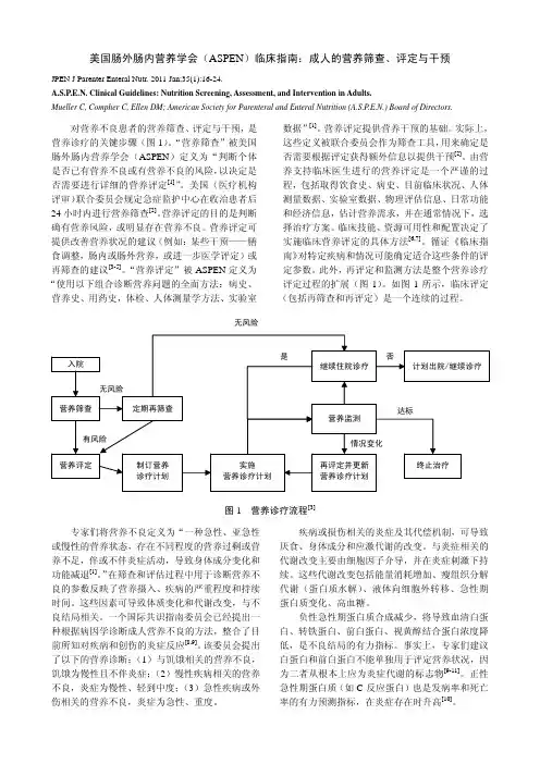
美国肠外肠内营养学会(ASPEN)临床指南:成人的营养筛查、评定与干预JPEN J Parenter Enteral Nutr. 2011 Jan;35(1):16-24.A.S.P.E.N. Clinical Guidelines: Nutrition Screening, Assessment, and Intervention in Adults.Mueller C, Compher C, Ellen DM; American Society for Parenteral and Enteral Nutrition (A.S.P.E.N.) Board of Directors.对营养不良患者的营养筛查、评定与干预,是营养诊疗的关键步骤(图1)。
“营养筛查”被美国肠外肠内营养学会(ASPEN)定义为“判断个体是否已有营养不良或有营养不良的风险,以决定是否需要进行详细的营养评定[1]”。
美国(医疗机构评审)联合委员会规定急症监护中心在收治患者后24小时内进行营养筛查[2]。
营养评定的目的是判断确有营养风险,或明显存在营养不良。
营养评定可提供改善营养状况的建议(例如:某些干预——膳食调整,肠内或肠外营养,或进一步医学评定)或再筛查的建议[3-5]。
“营养评定”被ASPEN定义为“使用以下组合诊断营养问题的全面方法:病史、营养史、用药史,体检、人体测量学方法、实验室数据”[1]。
营养评定提供营养干预的基础。
实际上,这些定义被联合委员会作为筛查工具,用来确定是否需要根据评定获得额外信息以提供干预[2]。
由营养支持临床医生进行的营养评定是一个严谨的过程,包括取得饮食史、病史、目前临床状况、人体测量数据、实验室数据、物理评估信息、日常功能和经济信息,估计营养需求,并在通常情况下,选择治疗方案。
临床技能、资源可用性和配置决定了实施临床营养评定的具体方法[6,7]。
循证《临床指南》对特定疾病和情况可能确定适合这些条件的评定参数。
晚期胃癌患者一线使用信迪利单抗联合SOX方案的疗效及疗效预测因子分析阴明妹① 冯江山① 赵正① 赵伟锋① 王朝杰① 【摘要】 目的:本研究旨在分析信迪利单抗联合SOX方案(替吉奥+奥沙利铂)一线治疗HER2阴性晚期胃癌的临床效果和安全性,并探讨影响患者生存期的疗效预测因子。
方法:回顾性分析2019年5月—2022年5月在河南省人民医院一线治疗接受信迪利单抗联合SOX方案的43例HER2阴性晚期胃癌患者的临床资料。
主要终点为客观有效率(ORR),次要终点包括疾病控制率(DCR)、无进展生存期(PFS)、总生存期(OS)、不良反应,并用Kaplan-Meier生存分析法及COX回归分析法对胃癌患者的疗效及多种疗效预测因子进行分析,用Log-rank检验进行显著性分析。
结果:43例HER2阴性晚期胃癌患者一线治疗接受了信迪利单抗联合SOX方案治疗,21例获得部分缓解(PR),15例病情稳定(SD),7例病情进展(PD)。
ORR和DCR分别为48.84%(21/43)和83.72%(36/43)。
中位PFS为8.6个月[95%CI(7.916,9.284)],中位OS为16.9个月[95%CI(14.078,19.722)]。
在信迪利单抗联合SOX方案一线治疗HER2阴性晚期胃癌患者的效果中分化程度、血小板与淋巴细胞比值(PLR)、治疗前美国东部肿瘤协作组活动状态(ECOG PS)评分组间的无进展生存期差异均有统计学意义(P<0.05),预后营养指数(PNI)、PLR、细胞程序性死亡-配体1(联合阳性分数)[PD-L1(CPS)]表达、ECOG PS评分组间的总生存期差异均有统计学意义(P<0.05)。
在单因素及多因素分析中,PD-L1(CPS)、ECOG PS为影响晚期胃癌患者OS的独立因素(P<0.05),PLR、ECOG PS为影响晚期胃癌患者PFS的独立因素(P<0.05)。
ation,migraUon and iuvvsion by targeting TRAF5iu colorectalcaucegj].BiochemBiopyys Res Commun,2212,510(5):799-7050[12]CHEN QY,DES MARAIS T,COSTA M.Dereaulatiov of SATB0iu carciuoyexesis with emppasis on miRNA-mediated control[J].Caniuoyexesis,258,45(3):596-450.[07]PATEL Y,SONI M,AWGULEWITSCH A,et al.OverexpresUon ofmiU-489derails mamma/hierarchy structure and indibitsHER2/kex-induced tumo/gexesis[J].Odcoyexe,228,38(3):245-453.[13]ZHAO T,QIC B,ZHOU S,et al.Expression of DEK iu paucreaticcauces and Us correlation with clinicopatSoloyicai features andproyuosis[J]■8Caucer,2219,15(4):910-909.[12]WEN Y,XU HN,PRIEETTE VIENEDGE L,et al.Optical ndopimaging detects the effects of DEK oncoyexe kuochkoou on theredop state of MDA-MB-050breast cauces cells[J].Mol Imaging BUU258,20(3):412-48.[22]LIE L,PIAO J GAO W,et al.DEK oves expression as as inde-pexdext biomarkes for poos proyuosis iu colorectal cauces[J].BMC Cauces,2513,13:367.[20]李景阳,孙丽梅,徐慧,等・DEK蛋白在非小细胞肺癌中的表达及临床意义[J]现代肿瘤医学,2512,20(20):3556-35590LI JY,SUN LM,XU H,et al.The clinical WgmUcadce of DEKproteiu expression iu uon-small cell lung cauces[J]•MoVeruOdcology,2212,24(20):3556-3559.(编校:张西敏)干扰NBS1表达抑制肝癌HepG2细胞增殖并促进凋亡肖瑞雪1,魏飞力2,徐忠法1,甄亚男1InteCering NBS1expression匚血巾匚恰proliferation and promotes apoptosis of livet cancer HepG2celloXIKO Ruixue1,WEI FeiU,XU Zhongfu1,ZHEN Yansu11Thr Thirg J^filiated Hospitai of Shandong First Medicai Universito(Affiliated Hospital ep ShanOong Acalema of Medical Sciences P, ShanOong Jinan250031,China;1Beijing Huhe op Henatolopa,Beijing Youan Hospital,Capital Medical Unwersito,Beijing100067, China.【Abstrvct i Objective:To invesUgato the ekect of NBS1knochdown oo yrollra/od and apoptosis of HepG2ceks.Methodt:NBS1specific small interference RNA(siNBSl)was transfected into HepG2cells,performed using Lipc-fectamine2000,with empty liposome as coowO grovp■The expressioo of NBS1was detected by RT-PCR and Western blot.The HepG2cell yrolifera/od was detected bs CCK-8methoV,and cell apoptosis was analyzed bs usingFCM.R csu U s:DiRerent codcekWatiods of siNBS1(10nmol/P,20nmol/L,50nmol/P)conlU indibit the expression ofNBS1gene at mRNA level in HepG2cells(P<0.05or P<0.01)■The highest codcekWa/od of UNBS1(50nmol/L)conlU significantly indibit the expression of NSB)K-8assas demodsWateX that the yrolifera/od of HepG2cells in siNBSl grovp transfected with diNerent codcekWatiods of siNBSl was lowec than that of the coowO grovp(P<0.05or P<0.01), and the yrolifera/od rate decreased most significantly aftec44h of Wansfectioo.FCM revealed thatthe apoptosis rate increased significantly aftec Wansfectioo(P<0.05or P<0.01),and was related to the concenWa-tioo.Conclusion:1ndibikod of NBS1gene expression can significantly inhibit the yrolifera/od and promote apoptosisof HepG2ceks.【Key words】NBS1,RNA interference,HepG2ceks,cek pndfen/od,cek apoptosisMoVern Oncoloyy2021,29(11):1859-1871【摘要】目的:探讨干扰NBS1基因表达对肝癌细胞HepG2增殖及凋亡的影响。
MEG3长链非编码RNA在胃癌组织中的表达及意义发表时间:2016-09-21T15:52:55.703Z 来源:《医师在线》2016年7月第14期作者:刘莉魏武杰李黎孙建海通讯作者[导读] 胃癌(gastric carcinoma,GC)是发生在消化道的恶性肿瘤,近年来在中国发病率排名第一。
(湖北省第三人民医院肿瘤科;湖北武汉430030)摘要:目的:检测胃癌中母系印记基因3(MEG3)长链非编码RNA的表达,探讨其与肿瘤发展的关系。
方法应用实时荧光定量PCR的方法检测87例胃癌及其配对癌旁正常胃粘膜组织中MEG3的表达,统计学分析其表达与肿瘤临床分期的关系。
结果统计学分析表明胃癌组织与配对癌旁正常组织比较MEG表达都有显著降低(P<0.01)。
结论MEG3在胃癌发生发展过程中表达有明显降低,与胃癌的发生有密切的关系。
关键词:胃癌;长链非编码RNA;MEG3Expression of MEG3 long non-coding RNA in Gastric Carcinomas and Its Clinical Significancy*LIU Li,WEI Wu-jie,LI Li,SUN Jian-haiThe Department of Oncology,The third people's Hospital of Hubei Provincel,Wuhan 430030,Hubei Province,China[Abstract]:Objective :To examine the MEG3 lncRNA expression in gastric carcinomas(GC)and correlate it with patient clinical status.Methods: Expression levels of MEG3 lncRNA were quantitated with stem-loop quantitative reverse transcription-PCR in 87 GC patients and paired adjacent normal tissues(ANTs),and correlated to the pathoclinical status of the patients.Results: Expression of MEG3 lncRNA was markedly decreased in GC tissues compared with ANTs(P<0.01).Conclusion:Expression of MEG3 lncRNA was attenuated in GCs and correlated closely with cancer progression.[Key words]:gastric carcinoma;long non-coding RNA;MEG3前言胃癌(gastric carcinoma,GC)是发生在消化道的恶性肿瘤,近年来在中国发病率排名第一[1]。
Advances in Clinical Medicine 临床医学进展, 2021, 11(4), 1782-1786Published Online April 2021 in Hans. /journal/acmhttps:///10.12677/acm.2021.114256妊娠晚期合并脾动脉瘤破裂1例并文献复习李美燕,宋志双,张淑慧,王福玲青岛大学附属医院,山东青岛收稿日期:2021年3月19日;录用日期:2021年4月18日;发布日期:2021年4月25日摘要脾动脉瘤是一种较为罕见的疾病,其发病率为0.01%~0.2%。
妊娠合并脾动脉瘤更为罕见,妊娠期由于多种因素的影响,脾动脉瘤易发生破裂,危及孕妇及胎儿生命安全。
现报告1例妊娠晚期合并脾动脉瘤破裂病例,探讨该病的临床特点及治疗方法,并回顾相关文献,以加深对该病的认识。
关键词妊娠,脾动脉瘤,破裂,病例报告Rupture of Splenic Artery Aneurysmin the Third Trimester of Pregnancy:A Case Report and Literature ReviewMeiyan Li, Zhishuang Song, Shuhui Zhang, Fuling WangAffiliated Hospital of Qingdao University, Qingdao ShandongReceived: Mar. 19th, 2021; accepted: Apr. 18th, 2021; published: Apr. 25th, 2021AbstractSplenic artery aneurysm is a rare disease with an incidence rate of 0.01%~0.2%. Pregnancy com-plicated with splenic aneurysm is rarer. Due to the influence of many factors, splenic aneurysm is prone to rupture during pregnancy, which endangers the life safety of pregnant women and fetus.This paper reports a case of rupture of splenic artery aneurysm in late pregnancy, discusses the clinical characteristics and treatment of the disease, and reviews the relevant literature to deepen the understanding of the disease.李美燕等KeywordsPregnancy, Splenic Artery Aneurysm, Rupture, Case ReportCopyright © 2021 by author(s) and Hans Publishers Inc.This work is licensed under the Creative Commons Attribution International License (CC BY 4.0)./licenses/by/4.0/1. 引言脾动脉瘤是脾动脉扩张形成的,脾动脉瘤破裂会导致严重的血流动力学性休克。
The c linical u se of MEG a ctivity a ssociated with b rain l esions J. B. Vieth1,2, H. Kober2,3, O. Ganslandt3, M. Möller2,3, and K. Kamada2 Departments of 1Biomedical Engineering, and 2Experimental Neuropsychiatry, and 3Clinic of Neurosurgery, University of Erlangen-Nürnberg, Germany1IntroductionBrain lesions may alter the surrounding brain tissue structurally by moving or compressing it, or by in-filtration or edema. Electrophysiological signs of the deteriorated function in these border zones can be focal slow (and fast) wave and epileptic activity in MEG (and EEG).Clinically it is of great interest to know the localiza-tion and the extent of these focal sources, but also the location and the extent of the evoked and event related activity of functionally important areas around brain lesions. So we developed, adapted and established clinical applications in neurosurgery and neurology with special reference to clinical rele-vance and acceptance.2Methods2.1Magnetic Source Imaging (MSI)2.1.1 B iomagnetic recording and source localiza-tion: From 1990 to 1994 we used the 37 channel system "Krenikon R" of Siemens, Erlangen, Germany (planar recording surface of 20 cm in diameter), and since 1995 the 2x37 channel system "MAGNES II R" of Biomagnetic Technologies Inc. (BTi), San Diego, CA, USA, (curved recording surface with a 14 cm open diameter). The transfer of the coordinates from the head to the recording device and to the magnetic resonance imaging (MRI) data set was done with our surface fit (edge detection algorithm) of the electrically measured head surface (Isotrack TM 3D-digitizer, Polhemus Navigation Sciences, Colches-ter, Vermont, USA) and the head surface which was reconstructed from the MR images. The transfer er-ror is less than 2 mm. The advantages are: (1) easy scanning of the head surface, (2) no need of fiducial points [19].We used the sphere as the volume conductor model [22]. The source model was - depending on the task - either the single current dipole model or a current distribution solution. In order to apply the single current dipole model in a more adequate way, the localization procedure is performed only on signal sections where one component predominantly de-scribes the signal. The principle component analysis (PCA) is used to select typically only 1-2 % of the whole recording signal, speeding up the source lo-calization procedure substantially [18].2.1.2 M EG multisource problem: The electric or magnetic fields of brain activity not only originate from the sources of interest but also from the rest of the brain. In order to reduce this "background activ-ity" we use besides the alpha blocking effect during the recording (eyes open) either one of two proce-dures:Following the localization of dipoles we use a spa-tial averaging, our Dipole-Density-Plot (DDP), which shows the spatial distribution of dipoles over the recording time. It works by a three dimensional convolution using a three dimensional Gaussian en-velope, that takes into account the localization un-certainty [18,38].Or we use a current density procedure, the CLSF (Current Localization by Spatial Filtering), which we adapted from Robinson and Rose [32]. Our ana-lyzing space (a sphere) consists of 7000 voxels which is adjusted in size and location to the area of interest [10]. The Current-Density-Plot (CDP) is our corresponding spatial averaging of the CLSF [13].2.2Functional Magnetic Resonance Imaging (fMRI) and Magnetic Resonance Spectroscopic Imaging (MRSI)For details of these comparing methods see for the fMRI, (1H MRSI) in [35], and for the MRSI in [16]. 3Results and Discussion3.1Clinical Applications: Normal activity The tool to localize the spatial relation of tumors and their border zones to the cortical somatosensory, motor, auditory and cortical speech areas are now routinely used in Erlangen for operation planning and intraoperative functional neuronavigation with either the Zeiss microscope neuronavigation system (MKM), or the Stealth pointer neuronavigation sys-tem [7].3.1.1 S omatosensory evoked and motor event re-lated responses: In neurosurgery the clinical useful-ness of the somatosensory magnetic evoked re-sponses (SEF = somatosensory evoked field) havebeen demonstrated [5,9,17,25,26,30,36]. A coupling of MSI results to the neuronavigator in image guided neurosurgery was also described [31,43]. The first motor related MEG response was the so called "Bereitschaftsfeld" of the supplementary motor area [4]. The localization of the directly motor induced MEG activity (MEF = motor evoked field) in the precentral gyrus followed [21].Up to June 2000 we localized in 137patients with tumors around the central sulcus successfully the somatosensory response in 131 cases (95,6 %) and the motor associated cortical responses in 68 out of 72 cases (94,4%), elicited by selfpaced finger movements (trigger obtained by rectified electro-myogram). The SEF-MEG results coincided in all patients with the intraoperatively evoked phase re-versal of the epicortically obtained evoked potentials [7,8,9].Figure1: Single dipole MSI source localization in the postcentral gyrus using the somatosensory evoked field (SEF) at 50 ms after the tactile stimulus of the right index finger (200 samples averaged) of a 65 years old female patient (wwa) with a meningeoma. A: display of the Stealth neuronavigator showing in a tangential plane the tumor and the MSI SEF source and the intraoperatively used pointer instru-ment. B: enlarged section of A, the central sulcus is shaded, and marked by CS and the SEF source by a white encircled spot (from [37]).86 patients out of the 137patients were operated by using the functional neuronavigation. 26 patients have not been operated on the basis of the MSI findings. In figure 1 an example is shown of the SEF dipole source in the postcentral gyrus in a patient with a meningeoma displayed by the Stealth neuro-navigator system (c.f. [7,8,9]).Figure 2 shows in a patient with a left astrocytoma an example of the MEF and the SEF dipole sources in the pre- and post-central gyrus respectively.3.1.2 M SI and functional MRI (fMRI): The "blood oxygenation level dependent contrast"(BOLD) [28] enables the functional magnetic reso-nance imaging (fMRI) [1], which is used to localize oxygenation differences caused by evoked or event related brain activity. Some fundamental differences between the MSI and the fMRI may result in misin-terpretations of the fMRI localization results. One of these is the different origin of the recorded signals: In MSI the neuronal areas will be localized. But In fMRI the venous branch of the blood supply indi-cates the oxygen level change [28,33]. Another im-portant difference is the time resolution: In fMRI it is in the order of seconds depending on the tissue diffusion and regulation time of oxygen. In MSI the time resolution is in the order of a millisecond. de-pending on the electric properties of the tissue and the recording equipment. So fMRI interpretations should be done with general caution.Figure 2: Single dipole MSI source localizations of the motor related source (MEF) in the precentral and of the somatosensory evoked field (SEF) in the postcentral gyrus of a 39 years old female patient (age) with a left astrocytoma. SEF and MEF dipole sources are marked respectively. The central sulcus is marked by CS in A. The SEF protocol was as in figure 1. The MEF source was localized at 100 ms after the movement onset of selfpaced brisk move-ments of the right index finger (100 samples aver-aged) (from [37]).The consequence of the two different principles of the signal origin is demonstrated in our two com-paring studies with 6 subjects [35] and 15 patients [27]. We found a dislocation of the evoked cortical responses obtained by MSI and fMRI typically by around 1 cm.3.1.3 E vent related speech responses: The clinical usefulness to localize the speech activated cortical areas was demonstrated [13,23,24,34]. In our ap-proach - similar to the WADA-Test [42] - we acti-vate visually by written words and pictograms of monosyllabic concrete objects via a glass fiber bun-dle from outside the shielded room. In addition tothe Wernicke area the Broca area can be activated by internally speaking of the prior recognised terms [11]. In order to enhance the average signal of the speech related signals meaningless pictograms were presented in another trial and were subtracted after averaging from the average of the speech related presentation [13,23,24].In Erlangen up to June 2000 we localized in 44pa-tients(37right and7left handed) with brain tumors the speech related cortical areas by using our aver-aging version of the CLSF, the CDP [23,24]. The handedness was determined by the Edinburgh Handedness Inventory [29]. We had a baseline group of 11 healthy subjects. In right handed people one high activity density was in the posterior part of the left superior temporal gyrus (Wernicke area) around 350 ms and with internal speaking in addi-tion in the left inferior frontal gyrus (Broca area) around 500-600 ms (methods c.f. [13]). 12 out of44 patients suffered preoperatively from transient or permanent speech disturbances.Figure3: Speech related MSI source localizations in A and somatosensory evoked field (SEF) in B of a 69 years old male patient (jza) with a left temporo-parietal glioma. The speech responses were elicited by presenting pictograms of monosyllabic concrete objects for 800 ms. The task was to recognise the meaning of the object and to speak internally the word of the object. The CLSF was determined of 250 averaged samples and displayed with isocontour lines. The first response appeared 340 ms after the onset of the presentation in the posterior part of the left superior temporal gyrus (Wernicke area) marked by W, and the second response was at 745 ms in the left inferior frontal gyrus (Broca area) marked by B. The SEF protocol was as in figure 1. In B the central sulcus is marked by CS (from [37]). In 43 patients(97,7%) the sensory speech area and in 38 patients (86,4%) also the motor speech area could be localized. 24 patients out of the 44patients were operated. 14 patients were operated by using the functional neuronavigation. None suffered from a postoperative deterioration of speech. 8 patients have not been operated on the basis of the MSI findings [23,24]. Figure 3 shows an example of the localization of the speech areas and the somatosen-sory evoked responses in a patient with a left tem-poro-parietal glioma.The simultaneous recording on both hemispheres allowed to determine the larger activity of the CLSF strength (= S, after regularization) by using the lat-erality index (LI):LI = (left S max – right S max) / (left S max + right S max)In 34 of 35 cases the activity was three to nine times larger on the left side and in 1 case three times larger on the right side [23,24]. Figure 4 shows an example of the CLSF hemispheric dominance.The invasive WADA-test [42] was used for confir-mation according to clinical needs restrictively only. In the 5 total cases the test agreed with the LI (4 left side, 1 right side). So this part of the WADA-test might be supplemented or replaced by the MSI ap-proach in the presurgical evaluation of patients. More comparing studies are necessary.Figure 4: CLSF-In-tensity (used for lat-erality index (LI))along lines acrossthe brain at the sen-sory speech response(W=Wernicke at 360ms), and at the mo-tor speech response(B=Broca at 410ms) of a 44 years oldmale patient with aleft temporal lowgrade glioma. A: testlines and CLSF iso-contourlines. B:CLSF- Intensity (af-ter regularization).3.2Clinical Applications: Abnormal activity 3.2.1 E valuation with structural lesions: The DDP and the CLSF (including the CDP) were tested up to June 2000 in 147 patients in the border zone of tu-mors and infarcts using focal slow wave activity (2-6 Hz)and in 88 cases using fast wave activity (12.5-30 Hz) [12]. 19 cases were additionally investigated using the magnetic resonance spectroscopy imaging(MRSI). On the basis of our results we can be sureto localize the center and at least the main portion of the functionally impaired area with or without visi-ble lesions in the MRI [15,16,38,40,41].3.2.2 E pileptogenic lesion: Normally the epilep-togenic zone is removed to cure the epilepsy. But the removal of the epileptogenic lesion (assumed to be the original cause of a seizure disorder) is also important for the clinical outcome [3]. Thus the functional localization of the epileptogenic lesion is of great interest. An advantage is: the signals of spontaneous interictal activity are easily to obtain compared to the acquisition of spikes or even a sei-zure. It appeared, that the spontaneous slow wave activity can be used to localize the epileptogenic lesion of focal epilepsies. [6,21,38,39,40].Figure 5: Current-Density-Plot (CDP) during the 10 minutes recording time of focal abnormal spontane-ous interictal activity in the border zone of a right frontal astrocytoma of a 67 years old female patient (ida) with grand mal epileptic seizures. In A: spikes, B: slow (2-6 Hz) and C: fast (12.5-30 Hz) wave ac-tivities. In B and C occurring spike/wave activity was eliminated in order to prevent contamination of the slow and fast wave spontaneous activity (from [37]).In our studies [39,40] with focal epilepsies we had one group of epileptic patients with structural le-sions (5 adults, 4 children) as the reason of the epi-lepsy, and the other group without any visible structural lesion (4 adults, 2 children). For localiza-tion enhancement both the DDP and the CDP have been used. Occurring spike/wave complexes were disregarded in the slow and fast wave activity analy-sis. The three different signal components (interictal epileptic spikes, slow and fast wave activity) of all patients gave a strong spatial coincidence of the DDP and CDP localizations. In the tumor patients the activity also coincided with the border zone of the tumors [39,40]. Figure 5 shows an example. Focal abnormal lesional activity even could be found associated with the (focal) Rolandic epilepsy of children [14]. We demonstrated that even in these cases an epileptogenic lesion may be present associ-ated with functional (psychopathological) deficits, in spite of that "per definitionem" no (visible struc-tural) lesion is associated with this disease in the MRI.So the localization of the epileptogenic lesion seems to be a valuable additional tool in the presurgical evaluation of epileptogenic patients, especially when no structural lesion is visible in the MRI. But more (multicenter) studies should be done to compare the localization of the epileptogenic lesion, interictal spikes and the seizure begin.3.2.3 C erebrovascular accidents: Cerebrovascular accidents account for around a quarter of the total mortality and the bulk rate of the disabled people. Therefore it would be of great value to have diag-nostic measures for an early detection of prestages. In our studies we found that the MSI is able to lo-calize not only the disturbed function around an in-farct (or tumor) but also that of an area without a visible lesion but with a functional and maybe re-versible impairment. These can be either transient ischemic attacks (TIA), or infarcts which are too small to be detected by the standard MRI resolution. Up to now we localized not only the pathological activity associated with brain infarcts in 23 patients, but also in 21 cases the activity associated with the penumbra of transient ischemic attacks (TIA) [16, 20,38,41].Thus also clinically silent reversible ischemic brain deficits can be localized in accordance to clinically silent brain infarcts [2]. This finding is of clinical importance for the decision, whether an extracranial stenosis of the internal carotid artery has caused deficits or not. And these deficits might be another indication for an endarterectomy [41].The detection and localization of such clinically si-lent deficits, caused by a carotid stenosis, needs a screening. So our finding is very helpful, that the abnormal activity of TIAs is lasting at least 4 weeks after the accident [20]. The localization of the pe-numbra of infarcts is also very important in relation with new therapeutic approaches (i.e. neuroprotec-tors), that prevent neurons to be damaged irreversi-bly. More clinical studies should verify the value of these diagnostic tools.3.2.4 B rain functions and metabolism: The ab-normal metabolic function of the brain lesion and the penumbra of infarcts and tumors can be local-ized by using the proton magnetic resonance spec-troscopic imaging (1H MRSI). So we combined theslow wave MSI and the MRSI in order to compare their spatial relation.3.2.4.1 B rain infarcts: We compared 12 patients with a brain infarct to 12 normal cases using the MEG slow wave dipole density (DDP) and the MRSI signal intensity of N-acetyl (NA) (marker for normal function of the brain) and the lactate (Lac) MRSI signal intensity (indicator of anaerobic me-tabolism) [16]. In the patients at least normal tissue, the border zone, and the bulk of the infarct were in-cluded in the analysis.Figure 6: Dipole-Density-Plot (DDP) of focal ab-normal spontaneous slow wave (2-6 Hz) activity of a 60 years old male patient (kfa) during the recording time of 10 minutes in the border zone of a left brain infarct in A. In B and C: additional overlay of a separately recorded proton magnetic resonance spectroscopic imaging ( 1H MRSI). In B: signals of lactate (Lac); in C: of N-acetyl (NA). Field of view (FOV) 200x200 mm, in A marked by a white line and indicated partly in C by the outer limit of the NA activity; 16x16 phase encoding; nominal in-plane resolution: 12.5 mm, point resolved spectroscopy (PRESS); TR: 1500 ms; TE 135 and 270 ms. Details in [16] (from [37]).The signal intensity of NA was significantly reduced in the regions with the highest slow wave activity but was well correlated interindividually with the dipole density (DDP) of the quantified maximum of slow waves. Though Lac was mildly accumulated in these regions, the Lac level had no correlation with slow wave magnetic activity.Figure 6 shows isocontourlines of the spatial distri-bution of the abnormal slow waves, the Lac and the NA activities of a patient with a brain infarct. Figure 7 shows an example of the same patient with the topographic development of the three activities (MSI, NA, Lac) along a line from normal to patho-logical tissue. It appears that the abnormal activity starts relatively far away from the infarct, typically 3 cm or more. [16].3.2.4.2 B rain tumors: We also compared 7 patients with common invasive and non invasive brain tu-mors (i.e. astrocytic tumor and menigeoma) to 10 healthy subjects [15]. The protocol was the same as in the infarct study.Figure 7: Intensity of abnormal spontaneous slow wave (2-6 Hz) activity, lactate (Lac) 1H MRSI activ-ity, and N-acetyl (NA) 1H MRSI activity of the same patient (kfa) as in figure 6 (left brain infarct) along a line from normal tissue into the bulk of the brain infarct. Same recording protocol as in figure 6. C: line seen in a T1 image. D: line seen in a T2. Enclo-sure in a white rectangular line marks the enlarged area in B. The line in B is in direct spatial relation to the three different activities in A. Details in [16] (from [37]).Focally increased slow (and fast) wave activities and epileptic spikes were observed in the neuronal area adjacent to the bulk of the tumor with a mild reduc-tion of NA and a slight accumulation of Lac. Lac intensity was less pronounced than in the infarct study. The bulk of the tumors was magnetically si-lent. The extension of the tumor border zone seems to depend on the invasiveness of the tumor, but it seems to be smaller than that of the infarcts, typi-cally about 2 cm. Figure 8 shows an example of the intensity of the three activities along a line from tis-sue of the border zone of a tumor through the tumor and back to tissue outside the tumor again [15].3.2.4.3 C onsequences: From the results of both studies we could assume, that preserved and metab-olically active cortical tissue in the border region of infarcts and tumors with remaining NA signal and the increased slow wave activity under lactic acido-sis (mild accumulation of Lac) could be one of the ischemic "penumbra" states [15,16]. So slow wavesources can serve as a marker to localize the penum-bra of infarcts and tumors. The clinical importance is to have a diagnostic tool to find and followup ar-eas of neurons, where in the case of infarcts thera-peutic measures (i.e. neuroprotectors) might prevent neurons to be damaged irreversibly. In the case of tumors an early detection of prestages of tumors can be possible.Figure 8: Intensity of abnormal spontaneous slow wave (2-6 Hz) activity, lactate (Lac) 1H MRSI activ-ity, and of N-acetyl (NA) 1H MRSI activity of a 53 years old female (mga) with a left meningeoma along a line from tissue in the border zone through one pole of the tumor and back to border zone tissue on the other side of the meningeoma. Same record-ing protocol as in figures 6 and 7. C: line seen in a T1 image. D: line seen in a T2. Enclosure in a white rectangular line marks the enlarged area in B. The line in B is in direct spatial relation to the three dif-ferent activities in A. Details in [15,16] (from [37]). 4ConclusionsIn our studies we could demonstrate: the localization of the function of eloquent cortical areas is well ac-cepted in functional image guided neurosurgery. The localization of the epileptogenic lesion is an addi-tional promising tool in the presurgical investigation of epileptic patients. The penumbra of transient is-chemic attacks (TIAs), of infarcts and of tumors can be localized. A possible screening for "asympto-matic TIAs" (clinically silent reversible neuronal deficit) might help in the prevention of strokes. In patients with infarcts the knowledge of the localiza-tion and the extent of the penumbra may serve as a basis to prevent the increase of irreversibly damaged tissue. In patients with tumors the localization of the border zone activity may serve as a tool of early de-tection or prestages of tumors. More clinical studies have to verify the value of these promising tools.References1.J.W. Belliveau, D.N. Kennedy Jr., R.C. McKin-stry, B.R. Buchbinder, R.M. Weisskoff, M.S.Cohen, J.M. Vevea, T.J. Brady, and B.R. Rosen, Functional mapping of the human visual cortex by magnetic resonance imaging, Science, 254, 716-719, 1991.2.L.R. Caplan, Silent brain infarcts, Cerebrovasc.Dis., 4 (Suppl 1), 32-40, 1994.3.G.D. Cascino, P.J. Kelly, F.W. Sharbrough, J.F.Hulihan, K.A. Hirschorn, and M.R. Trenerry, Longterm followup of stereotactic lesionectomy in partial epilepsy: Predictive factors and elec-troencephalographic results, Epilepsia,33, 639-644, 1992.4.L. Deecke, P. Weinberg, and P. Brickett, Mag-netic fields of the human brain accompanying voluntary movement: Bereitschaftsmagnetfeld, Exp. Brain Research,48, 144-148, 1982.5. C.C. Gallen, D.F. Sobel, T. Waltz, M. Aung, B.Copeland, B.J. Schwartz, E.C. Hirschkoff, andF.E. Bloom, Noninvasive presurgical neuro-magnetic mapping of somatosensory cortex, Neurosurgery, 33, 260-268, 1993.6. C.C. Gallen, E. Tecoma, V. Iragui, D.F. Sobel,B.J. Schwartz, and F.E. Bloom, Magnetic sourceimaging of abnormal low-frequency magnetic activity in presurgical evaluations of epilepsy, Epilepsia, 38, 452-460, 1997.7.O. Ganslandt, R. Fahlbusch, C. Nimsky, H. Ko-ber, M. Möller, R. Steinmeier, J. Romstöck, and J. Vieth, Functional neuronavigation with mag-netoencephalography: outcome in 50 patients with lesions around the motor cortex, Neurosur-gical Focus6, Article 3, 1999; and J. Neurosur-gery,91, 73-79, 1999.8.O. Ganslandt, R. Steinmeier, H. Kober, J. Vieth,J. Kassubek, J. Romstöck, C. Strauss, and R.Fahlbusch, Magnetic source imaging combined with image guided, frameless stereotaxy: a new method in surgery around the motor strip, Neu-rosurgery, 41, 621-627, 1997.9.O. Ganslandt, D. Ulbricht, H. Kober, J. Vieth,C. Strauss, and R. Fahlbusch, SEF-MEG lo-calization of somatosensory cortex as a method for presurgical assessment of functional brain area, Electroenceph. Clin. Neurophysiol., 46(Suppl.), 209-213, 1996.10.P. Grummich, H. Kober, and J. Vieth, Localiza-tion of the underlying currents of magnetic brain activity using spatial filtering, Biomed. Engi-neer. (Berlin), 37 (Suppl.2), 158-159, 1992. 11.P. Grummich, H. Kober, J. Vieth, J. Matschke,and O. Ganslandt, Sensory speech area inves-tigated by magnetoencephalography, Biomed.Engineer. (Berlin), 39(Suppl.), 129-130, 1994.12.P. Grummich, J. Vieth, H. Kober, H. Pongratz,D. Ulbricht, O. Ganslandt, Localization of focalspontaneous beta wave activity associated with structural lesions in the brain, in: Biomagnetism: Fundamental Research and Clinical Applica-tions, C. Baumgartner, L. Deecke, G. Stroink, and S.J. Williamson, Eds., Amsterdam: Elsevier Science IOS Press, 1995, pp 75-79.13.K. Kamada, H. Kober, M. Saguer, M. Möller,M. Kaltenhäuser, and J. Vieth, Responses to si-lent kanji reading of the native japanese and german in task subtraction magnetoencepha-lography, Cognitive Brain Res., 7, 89-98, 1998.14.K. Kamada, M. Möller, M. Saguer, J. Kassubek,M. Kaltenhäuser, H. Kober, M. Überall, H.Lauffer, D. Wenzel, and J. Vieth, Localization analysis of neuronal activities in benign rolandic epilepsy using magnetoencephalography, J.Neurological Sciences,154, 164-172, 1998. 15.K. Kamada, M. Möller, M. Saguer, O. Gan-slandt, M. Kaltenhäuser, H. Kober, and J. Vieth,A combined study of tumor-related brain lesionsusing magnetoencephalography and proton MR spectroscopic imaging, J. Neurological Sci-ences, (submitted for publication).16.K. Kamada, M. Saguer, M. Möller, K. Wicklow,M. Kaltenhäuser, H. Kober, and J. Vieth, Func-tional and metabolic analysis of cerebral ische-mia using magnetoencephalography and proton magnetic resonance spectroscopy, Annals of Neurology, 42, 554-563, 1997.17.K. Kamada, F. Takeuchi, S. Kuriki, O. Oshiro,K. Houkin, and H. Abe, Functional Neuro-surgical Stimulation with Brain Surface Mag-netic Resonance Images and Magneto-encephalography, Neurosurgery,33, 269-273, 1993.18.H. Kober, J. Vieth, P. Grummich, A. Daun, E.Weise, and H. Pongratz, The factor analysis used to improve the dipole-density-plot (DDP) to localize focal concentrations of spontaneous magnetic brain activity, Biomed. Engineer. (Ber-lin), 37(Suppl.2), 164-165, 199219.H. Kober, P. Grummich, and J. Vieth, Fit of thedigitized headsurface with the surface re-constructed from MRI-Tomography, in: Bio-magnetism: Fundamental Research and Clinical Applications, C. Baumgartner, L. Deecke, G.Stroink, and S.J. Williamson, Eds., Amsterdam: S.J. Elsevier Science IOS Press, 1995, pp 309-312.20.H. Kober, J.B. Vieth, C. Stippich, J.R. Kassu-bek, and R. Hopfengärtner,. Time course of ab-normal MEG activity associated with transient ischemic attacks, in: Biomag96: Proceedings of the Tenth International Conference on Biomag-netism, C.J. Aine, Y. Okada, G. Stroink, S.J.Swithenby, and C.C. Wood, Eds.. New York, Berlin, Heidelberg, Tokyo: Springer-Verlag, 2000, pp 1033-1036.21.J.D. Lewine, and W.W. Orrison, Magnetoen-cephalography and magnetic source imaging, Functional Brain Imaging, Mosby Year Book Inc., 1995, pp 369-417.22.J.W.H. Meijs, F.G.C. Bosch, M.J. Peters, andF.H. Lopes Da Silva, On the magnetic field dis-tribution generated by a dipolar current source situated in a realistically shaped compartment model of the head, Electroenceph. clin. Neuro-physiol.,66, 268-298, 198723.M. Möller, H. Kober, O. Ganslandt, C. Nimsky,and R. Fahlbusch,Functional mapping of speech evoked brain activity by magnetoen-cephalography and its clinical application, Bio-med. Engineer. (Berlin),44(Suppl.2), 159-161, 1999.24.M. Möller, H. Kober, O. Ganslandt, C. Nimsky,M. Kaltenhäuser, J. Vieth, and R. Fahlbusch, Speech relevant brain areas and their hemi-spheric dominance investigated by magnetoen-cephalography, Brain, (submitted for publica-tion)25.T. Morioka, T. Yamamoto, T. Katsuta, K. Fujii,and M. Fukui, Presurgical Three-Dimensional Magnetic Source Imaging of the Somatosensory Cortex in a Patient with a peri-Rolandic Lesion: Technical Note, Neurosurgery,34, 930-934, 1994.26.N. Nakasato, K. Seki, T. Kawamura, S. Ohtomo,A. Kanno, S. Fujita, K. Hatanaka, S. Fujiwara,T. Kayama, A. Takahashi, H. Jokura, T.Kumabe, H. Ikeda, K. Mizoi, and T. Yoshimoto, Cortical mapping using an MRI-linked whole head MEG system and presurgical decision making, Electroenceph. clin. Neurophysiol., 47(Suppl.), 333-341, 1996.27.C. Nimsky, C., O. Ganslandt, H. Kober, M.Möller, S. Ulmer, B. Tomandl, and R. Fahl-busch, Integration of Functional Magnetic Resonance Imaging Supported by Magnetoen-cephalography in Functional Neuronavigation, Neurosurgery, 44, 1249-1256, 1999.28.S. Ogawa, T.M. Lee, A.R. Kay, and D.W. Tank,Brain magnetic resonance imaging with contrast。