Vision and Robotics Perception Of Non-Rigid Motion Inference of Shape, Material and Force
- 格式:pdf
- 大小:384.45 KB
- 文档页数:7

AI and Robotics The Future is Now The advancement of AI and robotics has brought about a significant transformation in various aspects of our lives, shaping the way we work, communicate, and interact with technology. The integration of AI and robotics has enabled us to achieve tasks that were once considered impossible, leading to increased efficiency and productivity in different industries. However, this rapid progress has also sparked concerns about the potential consequences of relying too heavily on these technologies. One perspective on AI and robotics is the fear of job displacement and the impact on the workforce. As AI and robotics continue to evolve, there is a growing concern that automation will replace human workers, leading to mass unemployment and economic instability. While it is true that certain jobs may become obsolete due to automation, it is important to recognize the potential for new job opportunities to emerge in fields related to AI and robotics. By embracing these technologies and adapting to the changing landscape of the workforce, we can harness the benefits of automation while also creating new avenues for employment. Another perspective on AI and robotics is the ethical implications of developing autonomous systems with the ability to make decisions independently. As AI becomes more sophisticated, there are concerns about the potential for these systems to exhibit bias, discrimination, or even harm to humans. It is crucial for developers and policymakers to prioritize ethical considerations in the design and implementation of AI and robotics, ensuring that these technologies are used responsibly and in alignment with societal values. By establishing ethical guidelines and regulations, we can mitigate the risks associated with autonomous systems and promote trust in AI and robotics. On the other hand, proponents of AI and robotics argue that these technologies have the potential to revolutionize various industries and enhance our quality of life. From healthcare and transportation to manufacturing and entertainment, AI and robotics offer innovative solutions that can improve efficiency, accuracy, and safety. For example, in the field of healthcare, AI-powered diagnostic tools can help doctors make more accurate and timely diagnoses, leading to better patient outcomes. In the realm of transportation, autonomous vehicles have the potential to reduce traffic accidents and congestion, making our roads safer and moreefficient. Despite the benefits of AI and robotics, there are concerns about the potential consequences of overreliance on these technologies. As we become increasingly dependent on AI and robotics to perform tasks and make decisions on our behalf, there is a risk of losing control and autonomy over our lives. It is essential to strike a balance between leveraging the capabilities of AI and robotics and preserving human agency and decision-making. By fostering a collaborative relationship between humans and machines, we can maximize the benefits of automation while also maintaining our sense of agency and responsibility. In conclusion, the integration of AI and robotics into our daily lives presents both opportunities and challenges that require careful consideration and ethical reflection. While these technologies have the potential to revolutionize industries and improve efficiency, it is essential to address concerns about job displacement, ethical implications, and overreliance on automation. By embracing a human-centered approach to AI and robotics, we can harness the benefits of these technologies while also safeguarding our values and principles. As we navigate the future of AI and robotics, it is crucial to prioritize collaboration, transparency, and ethical responsibility to ensure a positive and sustainable impact on society.。
Artificial Intelligence AI is a rapidly evolving field that has captured the imagination of scientists,technologists,and the general public alike.It is a branch of computer science that aims to create machines capable of performing tasks that would typically require human intelligence.This includes learning,reasoning,selfcorrection,perception, and understanding natural language.Here is a detailed look at various aspects of AI and its implications for the future.Definition and ScopeAI is often divided into two main categories:narrow AI,which is designed to perform a specific task,and general AI,which aims to mimic human cognitive abilities across a wide range of tasks.The latter is still a theoretical concept,as current AI systems are limited in their scope and capabilities.History and DevelopmentThe concept of AI dates back to antiquity,with myths and stories of artificial beings endowed with consciousness and intelligence.However,the modern field of AI research began in the mid20th century,with the development of the first AI programs and the establishment of AI as a distinct academic discipline.Key TechnologiesAI relies on a variety of technologies,including machine learning,natural language processing,computer vision,and robotics.Machine learning,a subset of AI,involves the development of algorithms that enable computers to learn from and make predictions or decisions based on data.ApplicationsAI has found applications in numerous fields,such as healthcare,where it can assist in diagnosing diseases and personalizing treatment plans finance,where it can be used for fraud detection and risk assessment and transportation,with the development of autonomous vehicles.Ethical ConsiderationsThe rise of AI has raised several ethical questions,including concerns about privacy,the potential for job displacement,and the need for transparency in AI decisionmaking processes.It is essential to address these issues to ensure that AI is developed and usedresponsibly.Future ProspectsThe future of AI is both exciting and uncertain.On one hand,AI has the potential to revolutionize industries and improve our quality of life.On the other hand,there are concerns about the potential misuse of AI and the need to ensure that its development aligns with societal values.ConclusionAI is a complex and multifaceted field that is constantly evolving.As we continue to develop more advanced AI systems,it is crucial to consider the ethical implications and work towards creating AI that benefits humanity as a whole.In conclusion,Artificial Intelligence is not just a technological advancement but a transformative force that is reshaping our world.As we move forward,it is important to approach AI with a combination of enthusiasm for its potential and caution regarding its challenges.By doing so,we can harness the power of AI to create a better future for all.。
Robotics and ControlRobotics and control are two interconnected fields that have a significant impact on various industries and everyday life. The integration of robotics and control systems has revolutionized the way tasks are performed, from manufacturing and healthcare to entertainment and household chores. However, with the increasing complexity and autonomy of robots, there are also concerns and challenges that need to be addressed. One of the key benefits of robotics and control systems is the ability to automate repetitive and dangerous tasks, thereby improvingefficiency and safety. In manufacturing, robots are used to assemble products with precision and speed, leading to higher productivity and lower error rates. In the healthcare industry, robotic surgery systems enable minimally invasive procedures, reducing patient trauma and recovery time. Moreover, in the household, robotic vacuum cleaners and lawn mowers alleviate the burden of mundane chores, allowing individuals to focus on more meaningful activities. The integration of control systems in robotics plays a crucial role in ensuring the accuracy and reliability of robot operations. Control systems regulate the movement, speed, and force exerted by robots, enabling them to perform tasks with precision and consistency. For instance, in industrial automation, control systems are used to coordinate the motion of multiple robotic arms to execute complex tasks such as welding, painting, and assembly. In addition, control systems also contribute to the safety of robots by implementing emergency stop mechanisms and collision avoidance algorithms. Despite the numerous advantages of robotics and control systems, there are several challenges that need to be addressed to fully realize their potential. One of the major concerns is the ethical and societal implications of widespread automation. As robots continue to replace human labor in various industries, there is agrowing apprehension about job displacement and economic inequality. Moreover, the use of autonomous robots in warfare and surveillance raises ethical questions regarding the accountability and decision-making processes of these systems. Another challenge in the field of robotics and control is the need for robust and adaptive algorithms to handle complex and dynamic environments. While traditional control systems excel in predictable and structured settings, they may struggle to cope with uncertainties and variations in real-world scenarios. As a result, thereis a growing demand for advanced control algorithms that can adapt to changing conditions and learn from experience, such as reinforcement learning and neural network-based control. Furthermore, the integration of artificial intelligence (AI) in robotics and control introduces new opportunities and challenges. AI-powered robots have the potential to exhibit cognitive abilities, such as perception, reasoning, and decision-making, enabling them to perform tasks that were previously deemed unfeasible for machines. However, the deployment of AI in robotics also raises concerns about transparency, accountability, and bias, particularly in high-stakes applications such as autonomous vehicles and medical diagnosis. In conclusion, robotics and control systems have revolutionized various industries and aspects of daily life, offering numerous benefits such as improved efficiency, safety, and convenience. However, the widespread adoption of robotics and control also poses ethical, technical, and societal challenges that need to be carefully addressed. By considering multiple perspectives and embracing interdisciplinary collaboration, we can harness the full potential of robotics and control while mitigating the associated risks. As we continue to advance in these fields, it is crucial to prioritize ethical considerations, invest in research and development, and engage in open dialogue to ensure that robotics and control systems serve the best interests of humanity.。
Vision-Guided Robotics Visual Control Vision-guided robotics visual control is a crucial aspect of modern robotics technology. It involves the use of visual information to guide the movement and actions of robots in various applications such as manufacturing, logistics, healthcare, and even in space exploration. This technology has the potential to revolutionize the way robots interact with their environment, enabling them to perform complex tasks with precision and efficiency. However, there are challenges and requirements that need to be addressed to ensure the successful implementation of vision-guided robotics visual control.One of the key requirements for vision-guided robotics visual control is the need for high-quality and reliable visual data. This data is essential for the robots to accurately perceive and understand their surroundings, enabling them to make informed decisions and take appropriate actions. To achieve this, advanced imaging technologies such as cameras, depth sensors, and lidar systems are used to capture detailed and accurate visual information. Additionally, the development of sophisticated algorithms and software is necessary to process and analyze this visual data in real-time, allowing the robots to respond quickly and effectively to changes in their environment.Another important requirement for vision-guided robotics visual control is the need for robust and adaptable control systems. These systems are responsible for translating the visual information into actionable commands for the robots, allowing them to move, manipulate objects, and interact with their environment. To achieve this, the control systems must be capable of handling complex and dynamic visual inputs, while also being flexible enough to accommodate changes in the environment or task requirements. This requires the integration of advanced control algorithms, sensor fusion techniques, and machine learning models to enable the robots to adapt and respond to a wide range of visual stimuli.In addition to technical requirements, there are also practical and ethical considerations that need to be addressed when implementing vision-guided robotics visual control. For example, ensuring the safety and reliability of vision-guided robotic systems is of utmost importance, especially in applications where they interact with humans oroperate in dynamic and unpredictable environments. This requires the development of robust safety protocols, fail-safe mechanisms, and ethical guidelines to minimize the risk of accidents or unintended consequences.Furthermore, the widespread adoption of vision-guided robotics visual control raises important societal and economic considerations. As this technology becomes more prevalent in various industries, there is a growing need to address the potential impact on the workforce, job displacement, and the ethical implications of relying on automated systems for critical tasks. It is essential to consider the broader implications of this technology and work towards solutions that ensure a fair and equitable transition to a future where vision-guided robotics visual control plays a significant role.In conclusion, vision-guided robotics visual control holds great promise for advancing the capabilities of robotic systems in a wide range of applications. However, realizing this potential requires addressing a multitude of technical, practical, ethical, and societal requirements. By focusing on the development of high-quality visual data, robust control systems, safety and ethical considerations, and broader societal implications, we can work towards the successful implementation of vision-guided robotics visual control, unlocking new possibilities for the future of robotics technology.。

协作机器人技术的识别与感知方法介绍随着科技的不断发展,机器人在各个领域中扮演着越来越重要的角色。
其中,协作机器人技术的识别与感知方法是实现机器人与人类协调合作的关键。
本文将介绍协作机器人技术的识别与感知方法,从计算机视觉、机器学习以及传感器技术三个方面进行阐述。
一、计算机视觉计算机视觉是协作机器人识别与感知的重要技术之一。
通过摄像头和图像处理算法,机器人能够获取环境中的图像信息,进而识别和感知目标物体或人类行为。
常用的计算机视觉方法包括目标检测、目标跟踪、图像分割等。
目标检测是指在图像或视频序列中检测出特定目标的位置和边界框。
常用的目标检测算法包括基于神经网络的目标检测方法(如YOLO、Faster R-CNN)和传统的特征提取与分类方法(如Haar特征与级联分类器)。
目标检测能够使机器人在复杂环境中识别出各种物体,并做出相应的响应。
目标跟踪是指在视频序列中追踪目标随时间的变化。
机器人利用目标跟踪技术可以实时追踪物体的位置、运动轨迹等信息,从而做出适时的行为。
常见的目标跟踪算法包括基于相关滤波器的方法(如DCF、SAMF)和基于深度学习的方法(如Siamese网络)。
图像分割是指将图像划分为多个不同的区域,从而更好地理解图像中的对象。
图像分割可以分割出目标物体的边界,提取出局部特征,进一步帮助机器人实现更精确的感知。
常用的图像分割算法包括基于像素的方法(如k-means、MeanShift)和基于边缘的方法(如Canny边缘检测)。
二、机器学习机器学习是协作机器人感知方法中的重要技术支撑。
通过对大量数据的学习和归纳,机器能够从中抽取特征,并基于这些特征做出判断和决策。
常用的机器学习方法包括监督学习、无监督学习和强化学习。
监督学习是指通过输入样本和对应输出的标签,训练机器进行正确的分类和回归。
在协作机器人中,监督学习可以用来识别和感知人类行为,例如动作识别、姿态估计等。
常见的监督学习算法包括支持向量机(SVM)、决策树、神经网络等。
vision pro persona机理The Vision Pro Persona mechanism is a cutting-edge approach that integrates advanced artificial intelligence and machine learning techniques to create personalized and immersive experiences. This mechanism leverages vast amounts of data to understand and anticipate user preferences, behaviors, and emotions, enabling systems to adapt their interactions and presentations accordingly. Vision Pro Persona机制是一种前沿方法,它融合了先进的人工智能和机器学习技术,旨在创造个性化且沉浸式的体验。
该机制利用大量数据来理解和预测用户的偏好、行为和情感,从而使系统能够相应地调整其交互和呈现方式。
At the core of Vision Pro Persona lies a sophisticated algorithm that continuously analyzes and learns from user interactions. It identifies patterns and trends, extracting meaningful insights that inform personalized content delivery and interface design. This allows for a more intuitive and engaging user experience, tailored to the unique needs and preferences of each individual.Vision Pro Persona机制的核心是一个复杂的算法,它持续分析并从用户交互中学习。
双目视觉测量原理Stereo vision, also known as binocular vision, refers to the ability to perceive depth and three-dimensional structures by integrating the different images received by the left and right eyes. This is made possible by the brain using the differing signals received by each eye to calculate the distance and position of objects in the visual field. 双目视觉是指通过左右眼接收到的不同图像来感知深度和三维结构的能力。
这是通过大脑利用每只眼睛接收到的不同信号来计算视野中物体的距离和位置。
One of the key principles behind stereo vision is triangulation, wherein the brain uses the slight differences in the images receivedby the left and right eyes to calculate the distance to objects in the field of view. This is similar to the way in which surveyors use triangulation to measure distances and map out landscapes. 双目视觉的一个关键原理是三角测量,大脑利用左右眼接收到的图像之间的微小差异来计算视野中物体的距离。
这类似于测量员使用三角测量来测量距离和绘制出景观的方式。
机器视觉与其它领域的关系**机器视觉与其它领域的关系**Machine vision is a rapidly developing field that intersects with numerous other disciplines, each contributing to its advancement and broadening its application scope.机器视觉是一个快速发展的领域,它与众多其他学科相互交叉,每个学科都为其进步做出贡献,并扩大其应用范围。
One such discipline is computer science, which provides the theoretical frameworks and algorithms for image processing and analysis, enabling machine vision systems to accurately interpret and respond to visual information.其中一个学科是计算机科学,它为图像处理和分析提供了理论框架和算法,使机器视觉系统能够准确解读和响应视觉信息。
Artificial intelligence, another key area, plays a pivotal role in enhancing the capabilities of machine vision systems through deep learning and machine learning techniques.人工智能是另一个关键领域,它通过深度学习和机器学习技术,在提升机器视觉系统能力方面发挥着核心作用。
Robotics is closely aligned with machine vision, as vision systems are integral to robotic perception and navigation, enabling robots to interact with their environment more effectively.机器人技术与机器视觉紧密相连,因为视觉系统是机器人感知和导航的重要组成部分,使机器人能够更有效地与其环境进行交互。
Choosing between an Art Exhibition and aRobot PerformanceIn the realm of cultural and technological pursuits, the decision to attend an art exhibition or a robot performance often presents a dilemma. Both activities offer unique and engaging experiences, but their natures and appeal differ significantly. As such, choosing between them requires a careful consideration of personal interests, as well as an understanding of the value each event holds.Art exhibitions are a testament to the creativity and expression of human beings. They provide a window into the minds of artists, allowing visitors to immerse themselvesin a world of color, shape, and form. The paintings, sculptures, and installations displayed at theseexhibitions are often the culmination of months or even years of hard work and dedication. Attending an art exhibition is not just about admiring the finished pieces; it's also about appreciating the process, the struggle, and the joy that artists experience in their creative journey. On the other hand, robot performances offer a glimpse into the future of technology and its potential toentertain and amaze. These performances showcase the latest advancements in robotics, from lifelike movements to complex decision-making capabilities. Watching a robot dance, sing, or even engage in a conversation can be a thrilling experience, as it challenges our perception of what is possible with machines. Robot performances are not just about the technology itself; they are also about the vision and imagination of the people behind them.In comparing the two, it becomes apparent that the choice between an art exhibition and a robot performance depends heavily on one's personal preferences and interests. If you are drawn to the beauty and depth of artistic expression, then an art exhibition is likely to be the more satisfying option. However, if you are fascinated by the wonders of technology and its potential to revolutionizeour world, then a robot performance may hold greater appeal. Moreover, the choice can also be influenced by the context and circumstances surrounding the events. For instance, if you are visiting a city known for its rich artistic heritage, attending an art exhibition may be amore culturally significant experience. Conversely, if youare attending a technology conference or festival, a robot performance may be a more relevant and timely choice.In conclusion, the decision to attend an art exhibition or a robot performance is a personal one that should be based on your interests, preferences, and the context ofthe events. Both offer unique and enriching experiencesthat can broaden your horizons and enhance your understanding of the world. Whether you choose to immerse yourself in the creativity of art or be amazed by the wonders of technology, the important thing is to embracethe experience and allow it to inspire and enrich your life. **画展与机器人表演的选择**在文化与技术追求的领域里,决定是去参观画展还是观看机器人表演,常常成为一个让人难以抉择的问题。
科技发达英语作文In the modern era, the rapid advancement of technology has become an integral part of our lives. This essay will explore the impact of technology on various aspects of society andthe role it plays in shaping our future.The Digital RevolutionThe digital revolution has transformed the way we communicate, work, and learn. With the advent of smartphones and the internet, information is now at our fingertips. We can access a vast array of knowledge with just a few clicks, which has made education more accessible and personalized.Artificial IntelligenceArtificial Intelligence (AI) is another significant development that is reshaping our world. AI systems can perform tasks that would normally require human intelligence, such as visual perception, speech recognition, and decision-making. This has led to innovations in healthcare, where AI can assist in diagnosing diseases, and in the automotive industry, where self-driving cars are becoming a reality.Environmental ImpactTechnology also plays a crucial role in addressing environmental challenges. Renewable energy technologies, suchas solar panels and wind turbines, are becoming moreefficient and affordable, helping to reduce our reliance on fossil fuels and combat climate change.CybersecurityAs we become more interconnected, cybersecurity has become a critical concern. Protecting our digital infrastructure from cyber threats is essential to maintain the integrity of our data and systems. This has led to the growth of the cybersecurity industry, which is dedicated to developing and implementing protective measures.The Future of WorkThe future of work is also being shaped by technology. Automation and robotics are taking over tasks that were once performed by humans, leading to a shift in the job market. This requires us to adapt and develop new skills to stay relevant in an ever-evolving job landscape.ConclusionIn conclusion, technology is a driving force that continues to propel society forward. While it presents challenges, it also offers solutions and opportunities. As we embrace the technological advancements of today, it is essential to consider their implications and ensure that they are used responsibly for the benefit of all.。
现代电子技术Modern Electronics Technique2024年4月1日第47卷第7期Apr. 2024Vol. 47 No. 70 引 言随着我国制造强国战略逐步深化,人工智能制造[1]成为“中国制造2025”明确主攻方向,越来越多的工厂开始使用工业机器人和机器视觉实现自动化生产,使机器人能够适应更复杂的生产环境,提高生产效率。
作为实现人工智能制造和智慧城市基础[2]的手眼标定,是机器人和机器视觉进行协调工作的必要内容,通过重构三维场景获取相机坐标系和机器人坐标系之间的位姿关系,因此提升其精确度、标定范围和稳定性非常重要。
目前,标定的主要方法有主动视觉标定法、相机自标定法和传统相机标定法[3]。
主动视觉标定法优点在于不用借助标定物、稳定性强及算法简单,但成本高、设备昂贵;相机自标定法[4]灵活性强但精度低、鲁棒性差;传统相机标定法需要标定物辅助标定,但是算法足够成熟,鲁棒性强且操作简单[5⁃9]。
对于精度要求高和成本需要控制的场景,传统相机标定法能够满足要求。
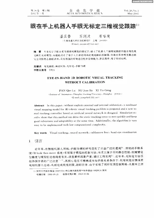
其中常用的方法有直线标定法、Tsai 两步法和张氏标定法,这面向工业机器人的非线性手眼标定方法研究胡宇鹏, 蒋年德(东华理工大学 信息工程学院, 江西 南昌 330013)摘 要: 手眼标定是机器人视觉领域中的一个关键技术,主要包括眼在手上和眼在手外两种标定方式。
标定的目的是得到相机坐标系与机器人坐标系之间的位姿关系,根据相机获取的图像重构三维场景,求出两个坐标系之间的转换参数,其结果将直接影响到机器人精准作业。
受当前镜头工艺水平和机器误差限制,相机采集的图像存在非线性畸变,原有的手眼标定方法存在精确度不足的缺点。
针对这个问题,文中提出面向工业机器人的非线性手眼标定方法,通过卷积原理使矩阵参数适应镜头下不同区域畸变的方法,减小相机镜头畸变影响。
通过实验验证表明,该方法能够提高手眼标定结果的精确度,标定后的平均误差为0.4 mm ,稳定性更强,可满足更多场景需求。
机器人创新特点英语作文Innovations in RoboticsRobotics has been a rapidly evolving field, constantly pushing the boundaries of what is possible. From the early industrial robots designed for repetitive tasks to the advanced humanoid robots of today, the innovation in this sector has been truly remarkable. As we delve into the unique features and advancements in robotics, it becomes evident that this field is not only transforming industries but also shaping the future of human-machine interaction.One of the most striking innovations in robotics is the development of autonomous systems. These robots are designed to operate independently, without the need for constant human supervision or control. This autonomy is achieved through the integration of sophisticated sensors, complex algorithms, and advanced decision-making capabilities. Autonomous robots can navigate through complex environments, adapt to changing conditions, and make real-time decisions based on the information they gather. This level of independence allows them to tackle tasks that would be challenging or even impossible for human operators, such as exploring hazardous environments or performing delicate surgicalprocedures.Another notable innovation in robotics is the incorporation of artificial intelligence (AI) and machine learning. These technologies have revolutionized the way robots perceive, process, and interact with the world around them. AI-powered robots can learn from their experiences, recognize patterns, and make informed decisions, enabling them to adapt and improve their performance over time. This adaptability is particularly valuable in dynamic and unpredictable environments, where the ability to respond to changing circumstances is crucial.The advancements in robotic manipulation and dexterity are also remarkable. Modern robots are equipped with highly precise and agile end-effectors, such as grippers and manipulators, that can perform intricate tasks with remarkable accuracy. This enhanced dexterity has opened up new possibilities in fields like surgery, where robotic systems can assist in delicate procedures that require a steady hand and a high degree of precision. Additionally, the development of soft robotics, which utilizes flexible and compliant materials, has expanded the range of applications for robots, allowing them to interact with fragile objects and even human beings in a more natural and intuitive manner.Another significant innovation in robotics is the integration ofhuman-robot interaction (HRI) technologies. Researchers have made significant strides in developing intuitive and natural ways for humans to communicate and collaborate with robots. This includes the use of natural language processing, gesture recognition, and even emotional intelligence, enabling robots to understand and respond to human cues and preferences. This enhanced interaction allows for a more seamless and efficient partnership between humans and machines, fostering greater trust and cooperation.The advancements in robotic sensing and perception have also been remarkable. Modern robots are equipped with a wide array of sensors, including vision, auditory, tactile, and even olfactory sensors, allowing them to perceive and interact with their environment in increasingly sophisticated ways. This enhanced sensory perception enables robots to navigate through complex environments, detect and avoid obstacles, and even recognize and respond to human emotions and behaviors.One of the most exciting developments in robotics is the emergence of collaborative robots, or "cobots," designed to work alongside human workers. These robots are designed to be safe, intuitive, and user-friendly, allowing for a seamless integration of human expertise and robotic capabilities. Cobots can assist human workers in tasks that are physically demanding, repetitive, or dangerous, freeing them up to focus on more complex and creative work. This collaborationbetween humans and robots has the potential to revolutionize various industries, from manufacturing to healthcare, by enhancing productivity, efficiency, and worker safety.The future of robotics holds even more promise, with researchers and engineers exploring the potential of bioinspired robotics, where the design and functionality of robots are inspired by nature and biological systems. This approach has led to the development of robots that can mimic the agility and adaptability of animals, opening up new avenues for exploration and problem-solving. Additionally, the integration of quantum computing and other emerging technologies into robotics is expected to further enhance the capabilities of these systems, enabling them to tackle increasingly complex tasks and solve problems that were previously out of reach.In conclusion, the innovations in robotics are truly remarkable, spanning a wide range of advancements in autonomy, artificial intelligence, manipulation, human-robot interaction, and sensing. These innovations are not only transforming industries but also paving the way for a future where humans and robots work together seamlessly, unlocking new possibilities and redefining the boundaries of what is possible. As we continue to push the limits of what robotics can achieve, the future holds endless possibilities forthe continued evolution and integration of these remarkable machines into our daily lives.。
In an era where technology is rapidly advancing,the concept of robots performing tasks traditionally reserved for humans is no longer a distant dream but a reality.One such fascinating development is the idea of robots dressing themselves.This innovation not only showcases the sophistication of artificial intelligence but also opens up a plethora of possibilities for various applications,from industrial automation to personal assistance.The journey of a robot learning to dress itself is a testament to the progress made in the field of robotics and AI.It involves a complex interplay of sensory perception,motor control,and cognitive processing. To begin with,the robot must be able to recognize different types of clothing and their respective parts.This requires the integration of advanced vision systems that can discern textures,patterns,and shapes.Once the clothing items are identified,the robot must then determine the correct sequence and method for dressing.This involves a deep understanding of the human bodys anatomy and the spatial relationships between the clothing and the body.For instance,a robot must know that a shirt is worn over the head and arms,and that pants are pulled up from the feet to the waist.The actual process of dressing is a delicate task that requires precise motor control.The robots arms must be able to mimic the dexterity of human hands,grasping the clothing items gently yet firmly,and maneuvering them into position.This is achieved through the use of sophisticated actuators and sensors that provide feedback on the force and position ofthe robots limbs.One of the most challenging aspects of a robot dressing itself is dealing with the variability in clothing sizes and styles.Unlike a human who can adjust their movements based on the feel of the fabric,a robot must rely on its sensors and algorithms to adapt to different types of clothing.This requires a high degree of flexibility and adaptability in the robots programming.The development of robots that can dress themselves has significant implications for various industries.In healthcare,for example,such robots could assist patients with limited mobility in getting dressed,providing them with greater independence and dignity.In the fashion industry, robots could be used to showcase clothing items on mannequins,offering a more dynamic and interactive shopping experience for customers.Moreover,the ability of robots to dress themselves also has potential applications in disaster relief and search and rescue operations.In such scenarios,robots could be deployed to quickly dress themselves in protective gear,allowing them to navigate hazardous environments and perform critical tasks with minimal risk to human life.It is worth noting,however,that the development of such technology is not without its challenges.The cost of developing and implementing advanced robotics systems can be prohibitive,and there are ethical considerations surrounding the potential displacement of human labor. Furthermore,the complexity of the task means that there is still muchroom for improvement in terms of speed,accuracy,and adaptability.In conclusion,the ability of robots to dress themselves represents a significant milestone in the field of robotics and AI.It showcases the potential for robots to perform intricate tasks that were once thought to be the exclusive domain of humans.As this technology continues to evolve, it is likely to have farreaching implications across various sectors,offering new opportunities for efficiency,accessibility,and innovation.However,it is crucial that we approach this development with a balanced perspective, considering both its benefits and potential drawbacks,and ensuring that it is used responsibly and ethically.。
Vision and RoboticsPerception O f N o n -R i g i d M o t i o n :Inference of Shape, M a t e r i a l and Force *A l e x P e n t l a n d a n d J o h n W i l l i a m s Vision Sciences Group, E15-410The M edia Lab, M .I.T.20 Ames St., Cambridge M A 02138A b s t r a c tMost non-rigid motion is much simpler than is generally thought, having many fewer degrees of freedom t h a n , for instance, 3-D shape. T h e relatively circumscribed nature of non-rigid motion can be seen by examining it f r o m the perspective of vibration modes. The fact t h a t a small number of parameters are sufficient to describe non-rigid motion mean that it is plausible to use sensory data to recover a nearly complete physical model of an object, so t h a t we can, for instance, predict its response to impinging forces. One perceptual task of considerable interest is estimating material properties such as stiffness, strength, and mass by watching, touching or listening to collisions. We derive equations which allow estimates of these material properties to be extracted f r o m visual and tactile data, and speculate on the use of aural data.1 I n t r o d u c t i o nNon-rigid m o t i o n seems to be very complex. W h e n an object is struck so t h a t it moves in a non-rigid, elastic manner, each point on the surface goes off in a different direction. It seems, therefore, t h a t a full description of non-rigid m o t i o n must have even more degrees of freed o m than a full description of shape. Despite this apparent complexity, however, people are often able to accurately predict the time course of objects experiencing non-rigid behavior, and are even able to infer material properties f r o m observing such m o t i o n.For instance, people can watch a tree l i m b swaying in the w i n d and make a good estimate of its stiffness, strength and mass. More commonly, when someone wants to determine the properties of an object they poke at it to see and feel it deform, and tap it to hear it resonate. From these visual, tactile, and auditory cues we are somehow able to ascertain material properties.In this paper we w i l l examine the finite element method of simulating the dynamics of collisions, and show t h a t it can be decomposed into simple, closed-form differential equations describing the object's vibration modes. We w i l l then show t h a t for most objects under *This research was made possible by NationalScience Foundation Grant No. IRI-87-19920 and by ARO Grant No. DAAL03-87-K-0005most conditions a relatively small number of modes are required to accurately describe how the object deforms as a function of time. Finally, we will show that for simple collisions we can estimate the object's material properties by observing these vibration modes using visual, tactile or even auditory data.2 B a c k g r o u n d : T h e F i n i t eElement M e t h o dT h e finite element method (F E M ) is a technique for simulating the dynamic behavior of an object. In the F E M the continuous variation of displacements throughout an object is replaced by a finite number of displacements at so-called nodal points. Displacements between nodal points are interpolated using a smooth function. Energy equations (or functionals) can then be derived in terms of the nodal unknowns and the resulting set of simultaneous equations can be iterated to solve for displacements as a function of impinging forces. In the dynamical case these equations may be w r i t t e n :Mu + D u + Ku = f (1)where u is a 3n x 1 vector of the (x, y, z) displacements of the n nodal points relative to the objects' center of mass, M , D and K are 3n by 3n matrices describing the mass, damping, and material stiffness between each point w i t h i n the body, and f is a 3n x 1 vector describing the (x ,y ,z ) components of the forces acting on the nodes. T h i s equation can be interpreted as assigning a certain mass to each nodal point and a certain material stiffness between nodal points, w i t h damping being accounted for by dashpots attached between the nodal points. The damping m a t r i x D is normally taken to be equal to s\M + s 2K for some scalars s 1, s 2. When S 1≠ 0 S 2 ≠ 0 this is called Raleigh damping, for s 2 = 0 it is called mass damping, and for s 1 = 0 stiffness damping.To calculate the result of applying some force f to the object one discretizes the equations in time, picking an appropriately small time step, solves this equation for the new u, and iterates u n t i l the system stabilizes. Direct (implicit) solution of the dynamic equations requires inversion the K m a t r i x , and is thus computationally expensive. Consequently explicit Euler methods (which are less stable, but require no m a t r i x inversion) are quite often applied.Even the explicit Euler methods are quite expensive, because the matrices M , D, and K are quite large: forPentland and Williams 15651566 Vision and RoboticsFigure 1: (a) A cylinder, (b) a linear deformation mode in response to compression, (c) a linear deformation mode in response to acceleration, (d) a quadratic modein response to a bending force, (e) superposition of bothlinear and quadratic modes in response to compression, (f) superposition of both linear and quadratic modes in response to acceleration.To obtain an accurate simulation of the dynamics of an object one simply uses linear superposition of these modes to determine how the object responds to a given force. Because Equation 4 can be solved in closed form, we have the result that for objects composed of linearly-deforming materials the non-rigid behavior of the objec t in response to an impulse forc e c an be solved in c losed form for any time t. The solution is discussed in Section 4. In environments w i t h more complex forces, however, analytic solution becomes cumbersome and so numerical solution is preferred. Either explicit or implicit solution techniques may be used to calculate how each mode varies w i t h time.Non-linear materials may be modeled by summing the modes at the end of each time step to f o r m the material stress state which can then be used to drive nonlinear plastic or viscous material behavior.4 Number Of Modes RequiredT h e modal representation decouples the degrees of free-dom w i t h i n the non-rigid dynamical system of Equation 1, but it does not reduced the t o t a l number of degrees of freedom. However once decoupled, we can separately analyze the various modes in order to determine which ones are required in order to obtain an accurate descrip-tion of an object's non-rigid dynamic behavior.T h e most i m p o r t a n t observation is t h a t modes asso-ciated w i t h high resonance frequencies normally have little effect on object shape. This is because:• The displacement amplitude for each mode is in-versely proportional to the square of the mode's resonance frequency. T h u s higher frequencies t y p i -cally have small amplitudes.1. 2.Figure 2: A ball coll • D a m p i n g is proportional to the mode's resonancefrequency. T h u s higher frequency vibrations dissi-pate quickly. • Frequencies are excited in proportion to the fre-quency content of the input force. T h e force gen-erated by simple collisions typically have a roughly Gaussian t i m e course, so that an individual reso-nance frequency / receives energy proportional toe -J 1° T h u s low frequencies typically receive moreenergy than high frequencies.The combination of these effects is that high-frequency modes have very little amplitude, and even less effect, in simple collisions. As a consequence much more efficient (and still accurate) simulation of an ob-ject's dynamics can be accomplished by discarding the small, high-frequency modes, and considering only the large-amplitude, low-frequency modes [5,6]. Exactly which modes to discard can determined by examining their associated eigenvalue, which determines the reso-nance frequency.Experimentally, we have found t h a t most common-place m u l t i -b o d y interactions can be adequately mod-eled by use of only rigid-body, linear, and quadratic strain modes. Figure 2, for instance, shows a example of a simulated non-rigid dynamic interaction: a ball col-liding w i t h a two-by-four. As can be seen, the interac-tion and resulting deformations look realistic despite theuse of only linear and quadratic modes.1Figure 1 also illustrates how use of linear and quadratic modes can accurately simulate non-rigid m o t i o n. Note, however, higher-order modes are required to accurately model the objects whose dimensions differ more than an order of magnitude.1Perhaps the most impressive fact about this example, however, is the speed of computation: Using a SymboUcs 3600 (with a speed of roughly one MIP), it requires only one CPU second to compute each second of simulated time!3. 4.iding with a two-by-four4.0.1 U s e o f F i x e d M o d e sNormally, in either the finite element or modal meth-ods, the mass, damping, and stiffness matrices are not recomputed at each time step. The use of fixed M , D, and K (or, equivalently, fixed modes) is well-justified as long as the material displacements are small. The defi-nition of "s m a l l /' however, is quite different for different modes. Because the eigenvalue decomposition in Equa-tion 2 performs a sort of principal-components analysis, it is the gross object shape (e.g., its low-order moments of inertia) determine the low-frequency modes, which as a consequence are quite stable. High-frequency modes are much less stable because they are determined by the fine features of the object's shape.In the standard finite element formulation the action of each mode is distributed across the entire set of equa-tions, so that one must recompute the mass and stiff-ness matrices as often as required by the very highest-frequency vibration modes. W h e n these high-frequency modes are discarded the mass, damping, and stiffness matrices need to be recomputed much less frequently. In most situations it is sufficient to use single, fixed set of low-frequency modes throughout an entire simulation.5 Estimation of MaterialPropertiesLet us imagine that we have seen the image sequence shown in Figure 2, and have been able to compute a full 3-D description of the object's shape at each instant. How can we estimate the material properties of these objects? The first step is to compute for each object a description that decomposes the object motion into its low-order modes.This can be accomplished by forming the vector p that describes each point on the object's surface, and then computing the matrices M, D, and K matrices using unit values for density and spring constant. Be-cause these matrices are determined by the vector p up to an overall constant, the eigenvectors found by solvingPentland and Williams 1567Equation 2 w i l l be identical regardless of the material properties (excepting, of course, non-linearly-behaving materials); only the eigenvalues depend upon the material properties. T h u s given the object's shape, we can directly determine Φ, the object's deformation modes.In this straightforward approach the matrices M, D, and K can become quite large, so that solution to Equation 2 becomes difficult. A more efficient method of determining Φ is be to fit either an eight or twenty point polygonal model to the sensed data (perhaps by use of the techniques described in reference [2]), and use the values of those points to construct a much smaller vector p. Given eight points we can form M, D, and K matrices that are 24 x 24 in size, and then solve Equation 2 to obtain the object's linear vibration modes. Given twenty points the matrices are 60 x 60, and produce both linear and quadratic vibration modes.A still more efficient scheme can be obtained by noting that the axes of the object can allow us to directly disentangle the action of the various modes, so that by estimating axis shape and length we can avoid solving Equation 2. This approach is described in more detail below.Given Φ and a description p(t) of the object's shape over time, we can directly decompose the object shape into a vector p(to) describing the object's shape at time / = t0a n d the amplitudes u(t) =Φl(p(t) —p(t0)) of each of the individual modes over time. The generic time behavior of each mode u i,(t) in response to an i mpinging force is given by Equation 4. T h e solution to this equation is which is graphed in Figure 3(b).Because the time behavior of u, is a function of M i,-, D i and K i, in simple situations we can recover the physical parameters of the object's material by measuring u i over time. This is particularly straightforward when the mode is underdamped, as in Figure 3, so that several cycles of deformation occur, because in this case we need only measure the frequency and amplitude of the deformation peaks. W h e n the mode is critically damped or overdamped only one peak occurs; however it is still possible to measure the material properties from peaks in the first derivative of the modal amplitude.For example, in the sequence of Figure 2 we can observe the bending of the two-by-four in response to the impact of the ball, as illustrated by Figure 4.If we plot the amplitude of this deformation mode in response to1568 Vision and Robotics5.1 E s t i m a t i o n of MassBy tracking geometry over time we can estimate the material properties up to an overall scale constant that depends upon the amount of mass involved in the particular vibration mode. The obvious question, then, is how much information is required to estimate the material density? To answer this question we surveyed the CRC Handbook, which lists the density of several hundred materials. We found that the listed densities could be clustered into four categories: metals, stones, biological materials, and woody (cellulose) materials. The range of densities for metals was roughly 7.0 to 10.0, for stone materials roughly 2.3 - 2.8, for biological materials (gums, resins, soap, etc.) roughly 0.9 - 1.2, and for woody materials (e.g., common woods, plant stems, etc.) roughly 0.4 - 0.6.Thus if the viewed material can be classified into one of these four categories, then it appears that the density can be estimated w i t h an accuracy of roughly ±10 percent. Consequently it appears that the force, mass, damping, and spring constants can also be estimated w i t h similar accuracy.5.2 Static L o a d i n gWhen a static load is applied to an object, a fixed deformation occurs. By examining Equation 4 we see that the amount of static deformation u i, is a function only of the loading force f i, and the stiffness constant K i associated w i t h the particular mode. Thus if we know the modes (either from analysis of the static shape or by the methods described in the next section) and the impinging force then we can determine the material stiffnessK i which is perhaps the most important of the basic material properties.In many situations, particularly when using a tactile sensor, this method of estimating material properties is probably the most practical.5.3 Speculation: E s t i m a t i o n f r o mO t h e r M o d a l i t i e sThe same ideas can be applied to the tactile and auditory senses: the modal vibration can be sensed eitherby touch or by sound (via coupling between the air andthe object surface). The notion of using a tactile sensorto produce a static measure of material stiffness has already been mentioned above. However a much stronger result can be achieved by using either tactile or auditory data given that we can apply a force f i so as to excite single mode i.In this case, because we knowthe force, we can measure the modal mass M, directly (from Equation 8), and thus obtain D, and K i, without knowledge of object geometry, modes, or density.For instance, if we "poke" or "tap" an object - exerta sharp blow normal to the surface - we can transfer most of the energy into a single, localized compression mode. To the extent that we are able to isolate a single mode, we need no knowledge of object geometry, modes,or density in order to estimate the physical parameters.In experiments where the sound spectrum produced by tapping has been measured it appears that most of the energy is indeed transferred into a single mode if the object's geometry is uniform in the area of the tap —e.g., the object is not hollow, and the tap occurs far from any discontinuity.6 Direct Observation of ModesWe have described a procedure of fitting data points, computing M, D, K. and then solving for Φ in order to obtain the object's vibration modes. Although mathematically sound, this procedure seems too complex and expensive to be useful in some applications. Similarly,the procedure is complex to be an account of human capabilities. Thus it is desirable to develop a theory thatis simpler even if less accurate.6.1 E s t i m a t i o n v i a s y m m e t r y axesThe first approach to direct observation of the modes depends on the observation that the object's axes of symmetry have a special status in modal analysis: theyare the singular lines (and planes) of the various vibration modes, i.e., the places along which various vibration modes cause no deformation. Thus along the axesof symmetry the actions of the different vibration modes become partially decoupled.Thus one direct way to estimate material propertiesis track the shape of symmetry axes over time. Time variation in the length of an axis is a function primarilyof linear compression modes, while the time variationin axis curvature is primarily a function of quadratic bending modes. Either the axis length or curvature canPentland and Williams 1569be tracked over time to produce a graph such as shown in Figure 3, and the material properties calculated by use of Equations 8. T h e simplicity of this method is its greatest virtue, however, in complex collisions the presence of many active vibration modes may destroy the accuracy of the approach.6.2 D i r e c t e s t i m a t i o n of m o d a la m p l i t u d e sA second approach is to fit the available shape data w i t h a simple volumetric model which can be parametrically deformed in any of the expected deformation modes. F i t t i n g the parameters of such a model to the sensor data provides a direct, simultaneous estimate of all of the modal amplitudes. Several variations on this ap-proach to extracting object geometry have been suc-cessfully demonstrated on range data [7,8,9,10]. As w i t h symmetry axes, the values of such a model's deforma-tion parameters can be tracked over time and material properties estimated by use of Equations 8. The advan-tage of this somewhat more computationally expensive approach is that is more likely to produce good esti-mates of modal amplitudes in relatively complex situa-tions.6.3 E s t i m a t i o n f r o m static i m a g e r yIn recent years both Pentland [11] and Ley ton [12] have suggested that an object's static shape can be analyzed to produce an abstract causal account of the object's history. T h a t is, t h a t a object's shape can be de-composed into a simple prototypical shape (a cube, a sphere) that has been modified by a sequence of forces or forming operations to achieve its present state. The advantage of this type of description is that produces a prototype-based representation t h a t can simplify object recognition [9] and which fits human psychological data[13].It can be seen, in retrospect, that both of these theo-ries were a t t e m p t i n g to capture the notion that objects have a limited repertoire of modal deformations. T h a t is, if one starts w i t h a fixed prototypical shape (a cylin-der, sphere, or cube for instance) an applies a series of forces to elastically deform that object, then in general the simplest possible description of the resulting shape is exactly the original shape plus the modal amplitudes that were produced by the impinging forces. Further, this description of object shape has considerable pre-dictive power, for it contains most of the information needed to estimate material properties, determine what forces were applied, and to predict the object's future dynamic behavior.7 S u m m a r yNon-rigid behavior is normally simpler than it appears from cursory examination of the F E M equations that describe such behavior. By breaking such motion into vibration modes, we can show that most of the degrees of freedom have very little energy or amplitude. Thus quite accurate descriptions of non-rigid behavior can beobtained by knowing the amplitude and phase of rela-tively few vibration modes.Using standard machine vision techniques the param-eters of these modes can be estimated f r o m sensory data. By tracking modal amplitudes across time (or, perhaps, even from analysis of static imagery!) we can then mea-sure material properties, predict future behavior, and perform other ecologically i m p o r t a n t tasks.R E F E R E N C E S[1][2][3][5][6][7] [8][9][10][11][12][13]Williams, J ., Musto, G., and Hawking, G., (1987) The Theoretical Basis of the Discrete Element M e t h o d , Numeri cal Methods in Engineering, The-ory, and Appli cation, R o t t e r d a m : Balkema Tub-ersTerzopoulos, D., P i a t t , J ., Barr, A., and Fleis-cher, K., (1987) Elastically deformable models, Proceedings of S 1G G R A P I I '87, Computer Graph-ics, Vol. 21, No. 3, pp 205-214.Williams, J. and Musto, G. (1987) Modal Methods for the Analysis of Discrete Systems, Computers and Geotec hnic s, Vol. 4, pp 1-19.Pentland, A., and W i l l i a m s , J. (1988) V i r t u a l Con-struction, Construc tion, Vol. 3, No. 3, pp. 12-22 Pentland, A. and W i l l i a m s , J., (1989) Good Vibra-tions: Modal Analysis for Graphics and Anima-tion, Proceedings of S I G G R A P H '89, Computer Graphics, Vol. 23, No. 3.Pentland, A., and W i l l i a m s , J . (1989) Fast Sim-ulation on Small Computers: Modal Dynamics Applied to Volumetric Models IEEE 20th Annual Conference on Simulation, May 4-5, Pittsburgh, PA.Pentland, A., (1988) Part segmentation for object recognition, Neural Computation, Vol. 1, No. 1 Pentland, A., (1988) A u t o m a t i c extraction of de-formable part models, M.I.T. Media Lab Vision Sciences Tec hnic al Note 104, J uly 1, 1988.Bajcsy, R. and Solina, F., (1987) Three-dimensional Object Representation Revisited, First International Conf. on Computer Vision, '87, J une 8-11, London, England.Bolt, T., and Gross, A., (1987) Recovery of Su-perquadrics from Depth Information, Pro ceedings of the AAA1 Workshop on Spatial Reasoning and Multi-Sensor Fusion, Oct. 1987, pp. 128-137Pentland, A. (1986) Perceptual Organization and the Representation of Natural Form, Artific ial In-telligence Journal, Vol. 28, No. 2, pp. 1-38.Ley ton, M. (1988) A Process-Grammar for Shape, Artificial Intelligen ce Journal, No. 34, pp. 213-247.Rosch, E. (1973) On the internal structure of per-ceptual and semantic categories. In Cognitive Development and the A cquisition of Language. Moore, T.E. (Ed.) New York: Academic Press.1570 Vision and Robotics。