Analyses of Multi-Way Branching Decision Tree Boosting Algorithms

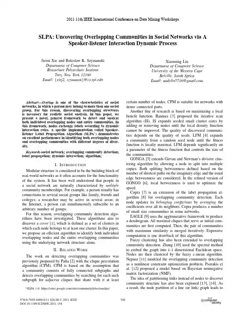
SLPA:Uncovering Overlapping Communities in Social Networks via A Speaker-listener Interaction Dynamic ProcessJierui Xie and Boleslaw K.Szymanski Department of Computer ScienceRensselaer Polytechnic InstituteTroy,New York12180 Email:{xiej2,szymansk}@Xiaoming Liu Department of Computer Science University of the Western Cape Belville,South Africa Email:andyliu5738@Abstract—Overlap is one of the characteristics of social networks,in which a person may belong to more than one social group.For this reason,discovering overlapping structures is necessary for realistic social analysis.In this paper,we present a novel,general framework to detect and analyze both individual overlapping nodes and entire communities.In this framework,nodes exchange labels according to dynamic interaction rules.A specific implementation called Speaker-listener Label Propagation Algorithm(SLPA1)demonstrates an excellent performance in identifying both overlapping nodes and overlapping communities with different degrees of diver-sity.Keywords-social network;overlapping community detection; label propagation;dynamic interaction;algorithm;I.I NTRODUCTIONModular structure is considered to be the building block of real-world networks as it often accounts for the functionality of the system.It has been well understood that people in a social network are naturally characterized by multiple community memberships.For example,a person usually has connections to several social groups like family,friends and colleges;a researcher may be active in several areas;in the Internet,a person can simultaneously subscribe to an arbitrary number of groups.For this reason,overlapping community detection algo-rithms have been investigated.These algorithms aim to discover a cover[1],which is defined as a set of clusters in which each node belongs to at least one cluster.In this paper, we propose an efficient algorithm to identify both individual overlapping nodes and the entire overlapping communities using the underlying network structure alone.II.R ELATED W ORKThe work on detecting overlapping communities was previously proposed by Palla[2]with the clique percolation algorithm(CPM).CPM is based on the assumption that a community consists of fully connected subgraphs and detects overlapping communities by searching for each such subgraph for adjacent cliques that share with it at least 1SLPA1.0:https:///site/communitydetectionslpa/certain number of nodes.CPM is suitable for networks with dense connected parts.Another line of research is based on maximizing a local benefit function.Baumes[3]proposed the iterative scan algorithm(IS).IS expands seeded small cluster cores by adding or removing nodes until the local density function cannot be improved.The quality of discovered communi-ties depends on the quality of seeds.LFM[4]expands a community from a random seed node until thefitness function is locally maximal.LFM depends significantly on a parameter of thefitness function that controls the size of the communities.GONGA[5]extends Girvan and Newman’s divisive clus-tering algorithm by allowing a node to split into multiple copies.Both splitting betweenness defined based on the number of shortest paths on the imaginary edge and the usual edge betweenness are considered.In the refined version of GONGO[6],local betweenness is used to optimize the speed.Copra[7]is an extension of the label propagation al-gorithm[8]for overlapping community detection.Each node updates its belonging coefficients by averaging the coefficients over all its neighbors.Copra produces a number of small size communities in some networks.EAGLE[9]uses the agglomerative framework to produce a dendrogram.All maximal cliques that serve as initial com-munities arefirst computed.Then,the pair of communities with maximum similarity is merged iteratively.Expensive computation is one drawback of this algorithm.Fuzzy clustering has also been extended to overlapping community detection.Zhang[10]used the spectral method to embed the graph into k-1dimensional Euclidean space. Nodes are then clustered by the fuzzy c-mean algorithm. Nepusz[11]modeled the overlapping community detection as a nonlinear constraint optimization problem.Psorakis et al.[12]proposed a model based on Bayesian nonnegative matrix factorization(NMF).The idea of partitioning links instead of nodes to discover community structure has also been explored[13],[14].As a result,the node partition of a line(or link)graph leads to2011 11th IEEE International Conference on Data Mining Workshopsan edge partition of the original graph.III.SLPA:S PEAKER-LISTENER L ABEL P ROPAGATIONA LGORITHMThe algorithm proposed in this paper is an extension of the Label Propagation Algorithm(LPA)[8].In LPA,each node holds only a single label that is iteratively updated by adopting the majority label in the neighborhood.Disjoint communities are discovered when the algorithm converges. One way to account for overlap is to allow each node to possess multiple labels as proposed in[15].Our algorithm follows this idea but applies different dynamics with more general features.In the dynamic process,we need to determine1)how to spread nodes’information to others;2)how to process the information received from others.The critical issue related to both questions is how information should be maintained. We propose a speaker-listener based information propagation process(SLPA)to mimic human communication behavior. In SLPA,each node can be a listener or a speaker.The roles are switched depending on whether a node serves as an information provider or information consumer.Typically, a node can hold as many labels as it likes,depending on what it has experienced in the stochastic processes driven by the underlying network structure.A node accumulates knowledge of repeatedly observed labels instead of erasing all but one of them.Moreover,the more a node observes a label,the more likely it will spread this label to other nodes (mimicking people’s preference of spreading most frequently discussed opinions).In a nutshell,SLPA consists of the following three stages (see algorithm1for pseudo-code):1)First,the memory of each node is initialized withthis node’s id(i.e.,with a unique label).2)Then,the following steps are repeated until the stopcriterion is satisfied:a.One node is selected as a listener.b.Each neighbor of the selected node sendsout a single label following certain speak-ing rule,such as selecting a random labelfrom its memory with probability propor-tional to the occurrence frequency of thislabel in the memory.c.The listener accepts one label from thecollection of labels received from neigh-bors following certain listening rule,suchas selecting the most popular label fromwhat it observed in the current step.3)Finally,the post-processing based on the labels inthe memories of nodes is applied to output thecommunities.SLPA utilizes an asynchronous update scheme,i.e.,when updating a listener’s memory at time t,some already updated Algorithm1:SLPA(T,r)[n,Nodes]=loadnetwork();Stage1:initializationfor i=1:n doNodes(i).Mem=i;Stage2:evolutionfor t=1:T doNodes.ShuffleOrder();for i=1:n doListener=Nodes(i);Speakers=Nodes(i).getNbs();for j=1:Speakers.len doLabelList(j)=Speakers(j).speakerRule();w=Listener.listenerRule(LabelList);Listener.Mem.add(w);Stage3:post-processingfor i=1:n doremove Nodes(i)labels seen with probability<r; neighbors have memories of size t and some other neighbors still have memories of size t−1.SLPA reduces to LPA when the size of memory is limited to one and the stop criterion is convergence of all labels.It is worth noticing that each node in our system has a memory and takes into account information that has been observed in the past to make current decision.This feature is typically absent in other label propagation algorithms such as[15],[16],where a node updates its label completely forgetting the old knowledge.This feature allows us to combine the accuracy of the asynchronous update with the stability of the synchronous update[8].As a result, the fragmentation issue of producing a number of small size communities observed in Copra in some networks,is avoided.A.Stop CriterionThe original LPA stop criterion of having every node assigned the most popular label in its neighborhood does not apply to the multiple labels case.Since neither the case where the algorithm reaches a single community(i.e., a special convergence state)nor the oscillation(e.g.,on bipartite network)would affect the stability of SLPA,we can stop at any time as long as we collect sufficient information for post-processing.In the current implementation,SLPA simply stops when the predefined maximum number of iterations T is reached.In general,SLPA produces relatively stable outputs,independent of network size or structure, when T is greater than20.B.Post-processing and Community DetectionSLAP collects only label information that reflects the underlying network structure during the evolution.The detection of communities is performed when the storedFigure 1.The convergence behavior of the parameter in LFR benchmarks with n=5000.y-axis is the ratio of the numbers of detected to true communities.Figure2.The execution time in second of SLPA in LFR benchmarks with k=20.n ranges from1000to50000.information is post-processed.Given the memory of a node, SLPA converts it into a probability distribution of labels. This distribution defines the strength of association to com-munities to which the node belongs.This distribution can be used for fuzzy communities detection[17].More often than not,one would like to produce crisp communities in which the membership of a node to a given community is binary, i.e.,either a node is in a community or not.To this end,a simple thresholding procedure is performed.If the probabil-ity of seeing a particular label during the whole process is less than a given threshold r∈[0,1],this label is deleted from a node’s memory.After thresholding,connected nodes having a particular label are grouped together and form a community.If a node contains multiple labels,it belongs to more than one community and is therefore called an overlapping node.In SLPA,we remove nested communities, so thefinal communities are maximal.As shown in Fig.1,SLPA converges(i.e.,producing similar output)quickly as the parameter r varies.The effective range is typically narrow.Note that the threshold is used only in the post-processing.It means that the dynamics of SLPA is completely determined by the network structure and the interaction rules.The number of memberships is constrained only by the node degree.In contrast,Copra uses a parameter to control the maximum number of memberships granted during the iterations.plexityThe initialization of labels requires O(n),where n is the total number of nodes.The outer loop is controlled by the user defined maximum iteration T,which is a small constant2.The inner loop is controlled by n.Each operation of the inner loop executes one speaking rule and one listening rule.For the speaking rule,selecting a label from the memory proportionally to the frequencies is,in principle, equivalent to randomly selecting an element from the array, 2In our experiments,we used T set to100.which is O(1)operation.For listening rule,since the listener needs to check all the labels from its neighbors,it takes O(K)on average,where K is the average degree.The complexity of the dynamic evolution(i.e.,stage1and2)for the asynchronous update is O(T m)on an arbitrary network and O(T n)on a sparse network,when m is the total number of edges.In the post-processing,the thresholding operation requires O(T n)operations since each node has a memory of size T.Therefore,the time complexity of the entire algorithm is O(T n)in sparse networks.For a naive implementation,the execution time on synthetic networks(see section IV)scales slightly faster than a linear growth with n as shown in Fig. 2.IV.E XPERIMENTS AND R ESULTSA.Benchmark NetworksTo study the behavior of SLPA for overlapping com-munity detection,we conducted extensive experiments on both synthetic and real-world networks.Table I lists the classical social networks for our tests and their statistics 3.For synthetic networks,we adopted the LFR benchmark [18],which is a special case of the planted l-partition model, but characterized by heterogeneous distributions of node degrees and community sizes.In our experiments,we used networks with size n=5000. The average degree is kept at k=10which is of the same order as most of the real-world networks we tested.The rest of the parameters are as follows:node degrees and commu-nity sizes are governed by the power laws,with exponents 2and1;the maximum degree is50;the community size varies between20and100;the mixing parameterµvaries from0.1to0.3,which is the expected fraction of links of a node connecting it to other communities.The degree of overlapping is determined by parameters O n(i.e.,the number of overlapping nodes)and O m(i.e., 3Data are available at /∼mejn/netdata/ and http://deim.urv.cat/∼aarenas/data/welcome.htmFigure 3.F-score for networks with n =5000,k =10,µ=0.1.Figure 4.F-score for networks with n =5000,k =10,µ=0.3.Figure 5.NMI for networks with n =5000,k =10,µ=0.1.Figure 6.Ratio of the detected to the known numbers of memberships for networks with n =5000,k =10,µ=0.1.Values over 1are possible when more memberships are detected than there are known to exist.Figure 7.Ratio of the detected to the known numbers of communities for networks with n =5000,k =10,µ=0.1.Values over 1are possible when more communities are detected than there are known toexist.Figure 8.NMI for networks with n =5000,k =10,µ=0.3.Figure 9.Ratio of the detected to the known numbers of memberships for networks with n =5000,k =10,µ=0.3.Values over 1are possible when more memberships are detected than there are known to exist.Figure 10.Ratio of the detected to the known numbers of communities for networks with n =5000,k =10,µ=0.3.Values over 1are possible when more communities are detected than there are known to exist.the number of communities to which each overlapping node belongs).We fixed the former to be 10%of the total number of nodes.The latter,the most important parameter for our test,varies from 2to 8indicating the diversity of overlapping nodes.By increasing the value of O m ,we create harder detection tasks.We compared SLPA with three well-known algorithms,including CFinder (the implementation of clique propagation algorithm [2]),Copra [7](another label propagation algo-rithm),and LFM [4](an algorithm expanding communities based on a fitness function).Parameters for those algorithmswere set as follows.For CFinder,k varied from 3to 10;for Copra,v varied from 1to 10;for LFM αwas set to 1.0which was reported to give good results.For SLPA,the maximum number of iterations T was set to 100and r varied from 0.01to 0.1to determine its optimal value.The average performances over ten repetitions are reported for SLPA and Copra.B.Identifying Overlapping Nodes in Synthetic Networks Allowing overlapping nodes is the key feature of over-lapping communities.For this reason,the ability to identify overlapping nodes is an essential component for quantifyingTable IT HE Q ov’S OF DIFFERENT ALGORITHMS ON REAL-WORLD SOCIAL NETWORKS. Network n k SLPA std r Copra std v LFM Cfinder k karate34 4.50.650.210.330.440.1830.420.523 dolphins62 5.10.760.030.450.700.0440.280.663 lesmis77 6.60.780.030.450.720.0520.720.634 polbooks1058.40.830.010.450.820.0520.740.793 football11510.60.700.010.450.690.0320.644 jazz19827.70.700.090.450.710.0510.557 netscience379 4.80.850.010.450.820.0260.460.613 celegans4538.90.310.220.350.210.1410.230.264 email11339.60.640.030.450.510.2220.250.463 CA-GrQc4730 5.60.760.000.450.710.0110.450.513 PGP10680 4.50.820.010.450.780.0290.440.573the quality of a detection algorithm.However,the node level evaluation is often neglected in previous work.Note that the number of overlapping nodes alone is not sufficient to quantify the detection performance.To provide more precise analysis,we define the identification of overlapping nodes as a binary classification problem.We use F-score as a measure of accuracy,which is the harmonic mean of precision(i.e.,the number of overlapping nodes detected correctly divided by the total number of detected overlapping node)and recall(i.e.,the number of overlapping nodes discovered correctly divided by the expected value of overlapping nodes,500here).Fig.3and4show the F-score as a functions of the number of memberships.SLPA achieves the largest F-score in networks with different levels of mixture,as defined byµ.CFinder and Copra have close performance in the test.Interestingly,SLPA has a positive correlation with O m while other algorithms typically demonstrate a negative correlation.This is due to the high precision of SLPA when each node may belong to many groups.C.Identifying Overlapping Communities in Synthetic Net-worksMost measures for quantifying the quality of a partition are not suitable for a cover produced by overlapping detec-tion algorithms.We adopted the extended normalized mutual information(NMI)proposed by Lancichinetti[1].NMI yields the values between0and1,with1corresponding to a perfect matching.The best performances in terms of NMI are shown in Fig.5and Fig.8for all algorithms with optimal parameters.The higher NMI of SLPA clearly shows that it outper-forms other algorithms over different networks structures (i.e.,with differentµ’s).Comparing the number of de-tected communities and the average number of detected memberships with the ground truth in the benchmark helps understand the results.As shown in Fig.6,7,9and10, both quantities reported by SLPA are closer to the ground truth than those reported by other algorithms.This is even the case forµ=0.3and large O m.The decrease in NMI is also relatively slow,indicating that SLPA is less sensitive to diversity of O m.In contrast,Copra drops fastest with the growth of O m,even though it is better than CFinder and LFM on average.D.Identifying Overlapping Communities in Real-world So-cial NetworksTo evaluate the performance of overlapping community detection in real-world networks,we used an overlapping measure,Q ov,proposed by Nicosia[19].It is an extension of Newman’s Modularity[20].As the Q ov function,we adopted the one used in[7],f(x)=60x−30.Q ov values vary between0and1.The larger the value is,the better the performance is.In this test,SLAP uses r in the range from0.02to0.45. Other algorithms use the same parameters as before.In Table I,the r,v and k are parameters of the corresponding algorithms.LFM usedµ=1.0.For SLPA and Copra,the algorithms repeated100times and recorded the average and standard deviation(std)of Q ov.As shown in Table I,SLPA achieves the highest Q ov in almost all the test networks,except the jazz network for which SLPA’s result is marginally smaller(by0.01)than that of Copra.SLPA outperforms Copra significantly(by>0.1) on Karate,celegans and email networks.On average,LFM and CFinder perform worse than either SLPA or Copra. To have better understanding of the output from the detection algorithms,we showed(in Table II)the statistics, including the number of detected communities(denoted as Com#),the number of detected overlapping nodes(i.e.,O d n) and the average number of detected memberships(i.e.,O d m). Due to the space limitation,we present only results from SLPA(Columns2to4)and CFinder(Columns5to7).It is interesting that all algorithms confirm that the di-versity of overlapping nodes in the tested social networks is small(close to2),although the number of overlapping nodes differs from algorithm to algorithm.SLPA seems to have a stricter concept of overlap and returns smaller number of overlapping nodes than CFinder.We observed that the numbers of communities detected by SLPA are ingood agreement with the results from other non-overlapping community detection algorithms.It is consistent with the fact that the overlapping degree is relatively low in these networks.V.C ONCLUSIONSIn this paper,we present a dynamic interaction process and one of its implementation,SLPA,to allow efficient and effective overlapping community detection.This process can be easily modified to accommodate different rules(i.e. speaker rule,listening rule,memory update,stop criterion and post-processing)and different types of networks(e.g., k-partite graphs).Interesting future research directions in-clude fuzzy hierarchy detection and temporal community detection.Table IIT HE STATISTICS OF THE OUTPUT FROM SLPA AND CF INDER.SLPA CFinder Network Com#O d n O d m Com#O d n O d mkarate 2.12 1.80 2.0032 2.00dolphins 3.44 1.24 2.0046 2.00lesmis 5.01 1.13 2.0043 2.33polbooks 3.40 1.30 2.0049 2.00football10.30 1.47 2.00136 2.00jazz 2.71 2.00 2.00639 2.05 netscience37.84 2.25 2.006548 2.33celegans 5.6814.42 2.006192 2.70email27.96 5.57 2.004183 2.12CA-GrQc499.940.02 2.00605548 2.40PGP105141 2.00734422 2.22A CKNOWLEDGMENTThis work was supported in part by the Army Re-search Laboratory under Cooperative Agreement Number W911NF-09-2-0053and by the Office of Naval Research Grant No.N00014-09-1-0607.The views and conclusions contained in this document are those of the authors and should not be interpreted as representing the official policies either expressed or implied of the Army Research Labora-tory,the Office of Naval Research,or the ernment.R EFERENCES[1] ncichinetti,S.Fortunato,and J.Kert´e sz,“Detecting theoverlapping and hierarchical community structure of complex networks,”New Journal of Physics,vol.11,p.033015,2009.[2]G.Palla,I.Der´e nyi,I.Farkas,and T.Vicsek,“Uncoveringthe overlapping community structure of complex networks in nature and society,”Nature,vol.435,pp.814–818,2005. [3]J.Baumes,M.Goldberg,M.Krishnamoorthy,M.Magdon-Ismail,and N.Preston,“Finding communities by clusteringa graph into overlapping subgraphs,”in IADIS,2005.[4] ncichinetti,S.Fortunato,and J.Kertesz,“Detecting theoverlapping and hierarchical community structure in complex networks,”New J.Phys.,vol.11,p.033015,2009.[5]S.Gregory,“An algorithm tofind overlapping communitystructure in networks,”Lect.Notes Comput.Sci.,2007. [6]S.G.,“A fast algorithm tofind overlapping communities innetworks,”Lect.Notes Comput.Sci.,vol.5211,p.408,2008.[7]S..Gregory,“Finding overlapping communities in networksby label propagation,”New J.Phys.,vol.12,p.10301,2010.[8]U.N.Raghavan,R.Albert,and S.Kumara,“Near lineartime algorithm to detect community structures in large-scale networks,”Phys.Rev.E,vol.76,p.036106,2007.[9]H.Shen,X.Cheng,K.Cai,and M.-B.Hu,“Detect overlap-ping and hierarchical community structure,”Physica A,vol.388,p.1706,2009.[10]S.Zhang,R.-S.Wangb,and X.-S.Zhang,“Identification ofoverlapping community structure in complex networks using fuzzy c-means clustering,”Physica A,vol.374,pp.483–490, 2007.[11]T.Nepusz,A.Petr´o czi,L.N´e gyessy,and F.Bazs´o,“Fuzzycommunities and the concept of bridgeness in complex net-works,”Phys.Rev.E,vol.77,p.016107,2008.[12]I.Psorakis,S.Roberts,and B.Sheldon,“Efficient bayesiancommunity detection using non-negative matrix factorisa-tion,”arXiv:1009.2646v5,2010.[13]Y.-Y.Ahn,J.P.Bagrow,and S.Lehmann,“Link communitiesreveal multiscale complexity in networks,”Nature,vol.466, pp.761–764,2010.[14]T.Evans and mbiotte,“Line graphs of weighted net-works for overlapping communities,”Eur.Phys.J.B,vol.77, p.265,2010.[15]S.Gregory,“Finding overlapping communities in networks bylabel propagation,”New J.Phys.,vol.12,p.103018,2010.[16]J.Xie and B.K.Szymanski,“Community detection using aneighborhood strength driven label propagation algorithm,”in IEEE NSW2011,2011,pp.188–195.[17]S.Gregory,“Fuzzy overlapping communities in networks,”Journal of Statistical Mechanics:Theory and Experiment,vol.2011,no.02,p.P02017,2011.[18] ncichinetti,S.Fortunato,and F.Radicchi,“Benchmarkgraphs for testing community detection algorithms,”Phys.Rev.E,vol.78,p.046110,2008.[19]V.Nicosia,G.Mangioni,V.Carchiolo,and M.Malgeri,“Extending the definition of modularity to directed graphs with overlapping communities,”J.Stat.Mech.,p.03024, 2009.[20]M.E.J.Newman,“Fast algorithm for detecting communitystructure in networks,”Phys.Rev.E,vol.69,p.066133,2004.。

anylsis英语解释### Analysis: A Comprehensive English Explanation#### IntroductionThe term "analysis" is widely used across various fields, including science, mathematics, business, and language arts.It refers to the process of examining, breaking down, or evaluating a subject or issue to understand its components, structure, or meaning.In this document, we will delve into the concept of analysis, providing a detailed English explanation to enhance your comprehension.#### Definition and SynonymsAt its core, "analysis" is the noun form derived from the Greek word "analysein," which means to break up or loosen.It encompasses the act of studying something in detail to understand its elements, function, or origin.Synonyms for analysis include:- Examination- Inspection- Evaluation- Review- Breakdown#### Usage in Various Contexts1.**Science and Mathematics**In scientific research, analysis is crucial for interpreting data and drawing conclusions.For example, a chemist might analyze a substance to determine its components.In mathematics, analysis can refer to the branch of math that deals with limits, functions, and the properties of real numbers.2.**Business and Finance**Business analysis involves examining processes, systems, or operations to improve efficiency or effectiveness.Financial analysis focuses on interpreting financial data to assess a company"s performance or predict its future prospects.3.**Language Arts**Literary analysis is the practice of examining a text closely to understand its themes, motifs, and deeper meanings.Linguistic analysis involves studying language structure, grammar, and syntax.#### Steps in the Analysis ProcessWhen conducting an analysis, the following steps are commonly followed:1.**Identification of Purpose**: Clearly define the reason for the analysis to guide the process.2.**Data Collection**: Gather relevant information, data, or materials necessary for the examination.3.**Examination**: Closely inspect the collected information,looking for patterns, connections, or anomalies.4.**Interpretation**: Make sense of the findings, often drawing comparisons or contrasts to other data or theories.5.**Analysis**: Break down the subject into its fundamental parts to understand how it works or why it is the way it is.6.**Conclusion**: Formulate conclusions based on the analysis, which may involve making recommendations or predictions.#### Importance of AnalysisAnalysis is essential because it:- Facilitates informed decision-making by providing a deeper understanding of a subject.- Helps solve complex problems by breaking them down into manageable parts.- Assists in identifying areas for improvement or optimization.- Provides a framework for critical thinking and evaluation.#### ConclusionIn summary, "analysis" is a multifaceted term that plays a pivotal role in various domains.Whether it"s used in scientific research, business strategy, or literary criticism, the process of analysis allows us to explore, understand, and draw meaningful conclusions from the world around us.Mastering the art of analysis can greatly enhance our ability to interpret, innovate, and make well-informed decisions.。

QUESTION ANSWERING AS A CLASSIFICATION TASK Edward Whittaker and Sadaoki FuruiDept.of Computer ScienceTokyo Institute of Technology2-12-1,Ookayama,Meguro-kuTokyo152-8552Japanedw,furui@furui.cs.titech.ac.jpABSTRACTIn this paper we treat question answering(QA)as a classifica-tion problem.Our motivation is to build systems for many lan-guages without the need for highly tuned linguistic modules.Con-sequently,word tokens and web data are used extensively but no explicit linguistic knowledge is incorporated.A mathematical model for answer retrieval,answer classification and answer length pre-diction is derived.The TREC2002QA task is used for system development where a confidence weighted score(CWS)of0.551 is obtained.Performance is evaluated on the factoid questions of the TREC2003QA task where a CWS of0.419is obtained which is in the mid-range of contemporary QA systems on the same task.1.INTRODUCTIONQuestion answering(QA),particularly in the style of the Text Re-trieval Conference(TREC)evaluations,has attracted significantly increased interest over recent years during which time“standard architectures”have evolved.More recently,there have been at-tempts to diverge from the highly-tuned,linguistic approaches to-wards more data-driven,statistical approaches[1,2,3,4,5,6]. In this paper,we present a new,general framework for question answering and evaluate its performance on the TREC2003QA task[7].QA,especially in the context of the Web,has been cited re-cently as the next-big-thing in search technology[8].Exploita-tion of the huge domain coverage and redundancy inherent in web data has also become a theme in many TREC participants’sys-tems e.g.[2,6].Redundancy in web data may be seen as effecting data expansion as opposed to the query expansion techniques and complex linguistic analysis often necessary in answering questions using afixed corpus,such as the AQUAINT corpus[9]where there are typically relatively few answer occurrences for any given ques-tion.The availability of large amounts of data,both for system train-ing and answer extraction logically leads to examining statistical approaches to question answering.In[1]a number of statistical methods is investigated for what was termed bridging the lexical gap between questions and answers.In[4]a maximum-entropy based classifier using several different features was used to deter-mine answer correctness and in[5]performance was compared against classifying the actual answer.A statistical noisy-channel model was used in[3]in which the distance computation between query and candidate answer sentences is performed in the space of parse trees.In[6]the lexical gap is bridged using a statistical translation model.Of these,our approach is probably most similar to[6]and the re-ranker in[5].Statistical approaches still under-perform the best TREC systems but have a number of potential advantages over highly tuned linguistic methods including robust-ness to noisy data,and rapid development for new languages and domains.In this paper we take a statistical,noisy-channel approach and treat QA as a whole as a classification problem.We present a new mathematical model for including all manner of dependencies in a consistent manner that is fully trainable if appropriate training data is available.In doing so we largely remove the need for ad-hoc weights and parameters that are a feature of many TREC sys-tems.Our motivation is the rapid development of data-driven QA systems in new languages where the need for highly tuned linguis-tic modules is removed.Apart from our new model for QA there are two major differences between our approach and many con-temporary approaches to QA.Firstly,we only use word tokens in our system and do not use WordNet,named-entity(NE)extraction, or any other linguistic information e.g from semantic analysis or from question parsing.Secondly,we use a search engine tofind relevant web documents and extract answers from the documents as a whole,rather than retrieving smaller text units such as sen-tences prior to determining the answers.2.CLASSIFICATION TASKIt is clear that the answer to a question depends primarily on the question itself but also on many other factors such as the person asking the question,the location of the person,what questions the person has asked before,and so on.Although such factors are clearly relevant in a real-world scenario they are difficult to model and also to test in an off-line mode,for example,in the context of the TREC evaluations.We therefore choose to consider only the dependence of an answer on the question,where each is considered to be a string of words and words,respectively.In particular,we hypoth-esize that the answer and its length depend on two sets offeatures and as follows:(1)where can be thought of as a set of features describing the“question-type”part of such as when,why,how, etc.and is a set of features comprising the “information-bearing”part of i.e.what the question is actuallyabout and what it refers to.For example,in the questions,Wherewas Tom Cruise married?and When was Tom Cruise married?theinformation-bearing component is identical in both cases whereasthe question-type component is different.Finding the best answer involves a search over all for theone which maximizes the probability of the above model:(2)This is guaranteed to give us the optimal answer in a maximumlikelihood sense if the probability distribution is the correct one.We don’t know this and it’s still difficult to model so we makevarious modeling assumptions to simplify ing Bayes’rule Equation(2)can be rearranged as:where,is the conditional probabilityof given the feature set and is an answer compensationweight that de-weights the contribution of an answer according toits frequency of occurrence in the language as a whole.isthe normalisation term.2.2.Filter modelThe question-type mapping function extracts-tuples()of question-type features from the question,such asHow,How many and When were.A set of single-word features is extracted based on frequency of occurrence inquestions in previous TREC question sets.Some examples in-clude:when,where,who,whose,how,many,high,deep,long etc.Modeling the complex relationship between and directly isnon-trivial.We therefore introduce an intermediate variable rep-resenting classes of example questions-and-answers(q-and-a)for drawn from the set,and to facilitate mod-eling we say that is conditionally independent of given asfollows:To obtain we use the Knowledge-Master questions and an-swers[10]and the questions and correct judgements from TRECQA evaluations prior to TREC2002by assigning each exampleq-and-a to its own unique class i.e.we do not perform clustering atall.Making a number of other similar modeling assumptions weobtain thefinal formulation for thefilter model:(5)where is a concrete class in the set of answer classes.Each class in is ideally a homogeneous and completeset of words for a given type of question,what is usually calledan answer-type in the literature,although in our model there isno explicit question-or answer-typing.For example,we expectclasses of river names,mountain names,presidents’names andcolors etc.The set of potential answers that are clustered,should ideally cover all words that might ever be answers to ques-tions.In keeping with our data-driven philosophy and related objec-tive to make our approach as language-independent as possible weuse an agglomerative clustering algorithm to derive classes auto-matically from data.The“seeds”for these clusters are chosen tobe the most frequent words in the AQUAINT corpus.The al-gorithm uses the co-occurrence probabilities of words in the samecorpus to group together words with similar co-occurrence statis-tics.For each word in some text corpus comprising unique words the co-occurrence probability is the probabil-ity of given occurring words away.If is positive,oc-curs after,and if negative,before.We then construct a vector of co-occurrences with maximum separation between words,as follows:Tofind the distance between two vectors,for efficiency,we use an distance metric:.The clustering algorithm is described in Algorithm2.1.The obtained classes are far from perfect in terms of completeness and homogeneity but were found to give reasonable results.initialize most frequent words to classes for i:=1tofor j:=1tocomputemove toupdate(6)3.EXPERIMENTAL WORKIn the question answering community the TREC QA task evalua-tions[9,7]are the de facto standard by which QA systems are as-sessed and in keeping with this,we use the500factoid questions from the2002TREC QA task for system development purposes and evaluate using the413factoid questions in the TREC2003 QA task.For training the model we use288,812example q-and-a from the Knowledge Master(KM)data[10]plus2,408q-and-a from the TREC-8,9and2001evaluations.For evaluations on the TREC2003data we also add in660example q-and-a from the TREC2002development set.The most frequentwords from the AQUAINT corpus were used to obtain for clusters using Algorithm2.1and .The maximum number of features used in the retrieval model was set to for reasons of memory efficiency.We use the Google search engine to retrieve the top doc-uments for each question.The question is passed as-is to Google except that stop words from the same list described at the begin-ning of Section2.1arefirst removed.Text normalization is mini-mal and involves only removing unnecessary markup,capitalising all words and inserting sentence boundaries.In all but one case,our evaluation is automatic and based on an exact character match between the answers provided by our sys-tem and the capitalized answers in the judgementfile.We consider two sets of correctness as defined in[9,7]where answers are either correct or not exact but where support correctness is ignored.We also look at several different metrics including the accuracy of cor-rect answers output in the top1,2and5answers,the number of correct and not exact answers in the top1position,and also at the mean reciprocal rank(MRR)and confidence-weighted score (CWS)defined in[9].CWS ranks each answer according to the confidence that the system assigns it and gives more weight to cor-rect answers with higher rank.3.1.DevelopmentAlthough in principle we could maximise the likelihood of each correct answer to optimise the system ourfinal objective is the number of correct answers.Consequently we use this as our opti-misation criterion on the set of500questions from the TREC2002 QA task.The optimised parameters were found to be:max, ,and.The best set of classes of those investigated was classes.Table1gives re-sults obtained on the development set.The1st column shows the different evaluation metrics.The2nd column gives the results for the best system(using the optimised parameters given above)and the3rd column gives results using only the retrieval model.TREC2002(dev.set TREC2003 Assessment Best Retrieval(evaluation set)criterion system model Exact0.276——correct16310496not exact202717—CWS0.5510.3050.419Table1.Performance on the development set(TREC2002)for best system and retrieval model only and performance on the eval-uation set(TREC2003)for the best development system.3.2.EvaluationWe use an identical setup for evaluation to the best system de-termined on the development set except that we also include the TREC2002q-and-a in.Two sets of results are shown in the final two columns of Table1.The4th column shows the results using an exact character match against the judgementfile provided by TREC and the last column shows the more realistic results of a human evaluation of the same answers.4.DISCUSSION AND ANALYSISAlthough our results on the development set are somewhat opti-mised they are in the mid-range of systems that participated in the TREC2002QA evaluation and compare very favourably with other mainly statistical systems[4,5].Indeed the top2and top5 results suggest there is scope for large improvements with limited system modifications.Moreover,the CWS scores indicate that an-swer confidence scoring is performed particularly well by our sta-tistical approach.On the evaluation set,however,the top1answer performance is reduced by29%compared to the development set performance.Below we examine where this difference in perfor-mance comes from.First of all,it is well known there are often disagreements as to what constitutes a correct answer and TREC tends to err on the side of marking an answer correct if the data supports it.Along these lines the human-scored results in thefinal column of Table1 indicate that our results are about18%better than doing an auto-matic evaluation would have us believe.In Table2we give the percentage of errors(i.e.incorrect an-swers according to the judgementfile)on questions in the evalu-ation set that can be attributed to each model or combination of models.The analysis of these errors is necessarily subjective but is interesting nonetheless.It shows,for example,that the retrieval component has contributed by far the most errors overall.Percentage of errors in each model combinationR L R&L R&F&L291129。

Governance Indicators:Where Are We, Where Should We Be Going?Daniel Kaufmann†Aart KraayProgress in measuring governance is assessed using a simple framework that distinguishes between indicators that measure formal rules and indicators that measure the practical application or outcomes of these rules.The analysis calls attention to the strengths and weaknesses of both types of indicators as well as the complementarities between them.It distinguishes between the views of experts and the results of surveys and assesses the merits of aggregate as opposed to individual governance indicators. Some simple principles are identified to guide the use and refinement of existing govern-ance indicators and the development of future indicators.These include transparently dis-closing and accounting for the margins of error in all indicators,drawing from a diversity of indicators and exploiting complementarities among them,submitting all indicators to rigorous public and academic scrutiny,and being realistic in expectations of future indicators.JEL codes:H1,O17Not everything that can be counted counts,and not everything thatcounts can be counted.—Albert Einstein Most scholars,policymakers,aid donors,and aid recipients recognize that good governance is a fundamental ingredient of sustained economic development.This growing understanding,initially informed by a very limited set of empirical measures of governance,has spurred intense interest in developing more refined, nuanced,and policy-relevant indicators of governance.This article reviews progress in measuring governance,emphasizing empirical measures explicitly designed to be comparable across countries and in most cases over time.The goal is to provide a structure for thinking about the strengths and weaknesses of different types of governance indicators that can inform both the use of existing indicators and ongoing efforts to improve them and develop new ones.1 Thefirst section of this article reviews definitions of governance.Although there are many broad definitions of governance,the degree of definitional disagreement#The Author2008.Published by Oxford University Press on behalf of the International Bank for Reconstruction and Development/THE WORLD BANK.All rights reserved.For permissions,please e-mail:journals.permissions@ doi;10.1093/wbro/lkm012Advance Access publication January31,200823:1–30can easily be overstated.Most definitions appropriately emphasize the importance of a capable state that is accountable to citizens and operating under the rule of law.Broad principles of governance along these lines are naturally not amenable to direct observation and thus to direct measurement.As Albert Einstein noted,“Not everything that counts can be counted.”Many different types of data provide infor-mation on the extent to which these principles of governance are observed across countries.An important corollary is that any particular indicator of governance can usefully be interpreted as an imperfect proxy for some unobserved broad dimension of governance.This interpretation emphasizes throughout this review a recurrent theme that there is measurement error in all governance indicators, which should be explicitly considered when using these kinds of data to draw conclusions about cross-country differences or trends in governance over time.The second section addresses what is measured.The discussion highlights the distinction between indicators that measure specific rules“on the books”and indi-cators that measure particular governance outcomes“on the ground.”Rules on the books codify details of the constitutional,legal,or regulatory environment; the existence or absence of specific agencies,such as anticorruption commissions or independent auditors;and so forth—components intended to provide the key de jure foundations of governance.On-the-ground measures assess de facto govern-ance outcomes that result from the application of these rules(Dofirmsfind the regulatory environment cumbersome?Do households believe the police are corrupt?).An important message in this section concerns the shared limitations of indicators of both rules and outcomes:Outcome-based indicators of governance can be difficult to link back to specific policy interventions,and the links from easy-to-measure de jure indicators of rules to governance outcomes of interest are not yet well understood and in some cases appear tenuous at best.They remind us of the need to respect Einstein’s dictum that“not everything that can be counted counts.”The third section examines whose views should be relied on.Indicators based on the views of various types of experts are distinguished from survey-based indi-cators that capture the views of large samples offirms and individuals.A category of aggregate indicators that combine,organize,provide structure,and summarize information from these different types of respondents is examined.The fourth section examines the rationale for such aggregate indicators,and their strengths and weaknesses.The set of indicators discussed in this survey is intended to provide leading examples of major governance indicators rather than an exhaustive stocktaking of existing indicators in this taxonomy.2A feature of efforts to measure governance is the preponderance of indicators focused on measuring de facto governance out-comes and the paucity of measures of de jure rules.Almost by necessity,de jure rules-based indicators of governance reflect the views or judgments of experts.In 2The W orld Bank Research Observer,vol.23,no.1(Spring2008)contrast,the much larger body of de facto indicators captures the views of both experts and survey respondents.The article concludes with a discussion of the way forward in measuring govern-ance in a manner that can be useful to policymakers.The emphasis is on the importance of consumers and producers of governance indicators clearly recogniz-ing and disclosing the pervasive measurement error in any type of governance indi-cators.This section also notes the importance of moving away from oft-heard false dichotomies,such as“subjective”or“objective”indicators or aggregate or disaggre-gated ones.For good reason,virtually all measures of governance involve a degree of subjective judgment,and different levels of aggregation are appropriate for differ-ent types of analysis.In any case,the choice is not either one or the other,as most aggregate indicators can readily be unbundled into their constituent components. What Does Governance Mean?The concept of governance is not a new one.Early discussions go back to at least 400BCE,to the Arthashastra,a treatise on governance attributed to Kautilya, thought to be the chief minister to the king of India.Kautilya presents key pillars of the“art of governance,”emphasizing justice,ethics,and anti-autocratic ten-dencies.He identifies the duty of the king to protect the wealth of the state and its subjects and to enhance,maintain,and safeguard this wealth as well as the inter-ests of the kingdom’s subjects.Despite the long provenance of the concept,no strong consensus has formed around a single definition of governance or institutional quality.For this reason, throughout this article the terms governance,institutions,and institutional quality are used interchangeably,if somewhat imprecisely.Researchers and organizations have produced a wide array of definitions.Some definitions are so broad that they cover almost anything(such as the definition“rules,enforcement mechanisms, and organizations”offered in the World Bank’s W orld Development Report2002: Building Institutions for Markets).Others,like the definition suggested by North (2000),are not only broad but risk making the links from good governance to development almost tautological:“How do we account for poverty in the midst of plenty?...We must create incentives for people to invest in more efficient tech-nology,increase their skills,and organize efficient markets....Such incentives are embodied in institutions.”Some of the governance indicators surveyed capture a wide range of develop-ment outcomes.While it is difficult to draw a line between governance and the ultimate development outcomes of interest,it is useful at both the definitional and measurement stages to emphasize concepts of governance that are at least some-what removed from development outcomes themselves.An early and narrower Kaufmann and Kraay3definition of public sector governance proposed by the World Bank is that “governance is the manner in which power is exercised in the management of a country’s economic and social resources for development”(World Bank1992, p.1).This definition remains almost unchanged in the Bank’s2007governance and anticorruption strategy,with governance defined as“the manner in which public officials and institutions acquire and exercise the authority to shape public policy and provide public goods and services”(World Bank2007,p.1).Kaufmann,Kraay,and Zoido-Lobato´n(1999a,p.1)define governance as“the traditions and institutions by which authority in a country is exercised.This includes the process by which governments are selected,monitored and replaced; the capacity of the government to effectively formulate and implement sound policies;and the respect of citizens and the state for the institutions that govern economic and social interactions among them.”Although the number of definitions of governance is large,there is some con-sensus.Most definitions agree on the importance of a capable state operating under the rule of law.Interestingly,comparing the last three definitions cited above,the one substantive difference has to do with the explicit degree of empha-sis on the role of democratic accountability of governments to their citizens.Even these narrower definitions remain sufficiently broad that there is scope for a wide diversity of empirical measures of various dimensions of good governance.The gravity of the issues dealt with in these definitions of governance suggests that measurement is important.In recent years there has been debate over whether such broad notions of governance can be usefully measured.Many indicators can shed light on various dimensions of governance.However,given the breadth of the concepts,and in many cases their inherent unobservability,no single indicator or combination of indicators can provide a completely reliable measure of any of these dimensions of governance.Rather,it is useful to think of the various specific indi-cators discussed below as all providing imperfect signals of fundamentally unobser-vable concepts of governance.This interpretation emphasizes the importance of taking into account as explicitly as possible the inevitable resulting measurement error in all indicators of governance when analyzing and interpreting any such measure.As shown below,however,the fact that such margins of error arefinite and still allow for meaningful country comparisons across space and time suggests that measuring governance is both feasible and informative.Governance Rules or Governance Outcomes?This section examines both the rules-based and outcome-based indicators of gov-ernance.A rules-based indicator of corruption might measure whether countries have legislation prohibiting corruption or have an anticorruption agency. 4The W orld Bank Research Observer,vol.23,no.1(Spring2008)An outcome-based measure could assess whether the laws are enforced or the anticorruption agency is undermined by political interference.The views offirms, individuals,nongovernmental organizations(NGOs),or commercial risk-rating agencies could also be solicited regarding the prevalence of corruption in the public sector.To measure public sector accountability,one could observe the rules regarding the presence of formal elections,financial disclosure requirements for public servants,and the like.One could also assess the extent to which these rules operate in practice by surveying respondents regarding the functioning of the institutions of democratic accountability.Because a clear line does not always distinguish the two types of indicators,it is more useful to think of ordering different indicators along a continuum,with one end corresponding to rules and the other to ultimate governance outcomes of interest.Because both types of indicators have their own strengths and weak-nesses,all indicators should be thought of as imperfect,but complementary proxies for the aspects of governance they purport to measure.Rules-Based Indicators of GovernanceSeveral rules-based indicators are used to assess governance(tables1and2). They include the Doing Business project of the World Bank,which reports detailed information on the legal and regulatory environment in a large set of countries;the Database of Political Institutions,constructed by World Bank researchers,and the POLITY-IV database of the University of Maryland,both of which report detailed factual information on features of countries’political systems;and the Global Integrity Index(GII),which provides detailed information on the legal framework governing public sector accountability and transparency in a sample of41countries,most of them developing economies.Atfirst glance,one of the main virtues of indicators of rules is their clarity.It is straightforward to ascertain whether a country has a presidential or a parliamen-tary system of government or whether a country has a legally independent anti-corruption commission.In principle,it is also straightforward to document details of the legal and regulatory environment,such as how many legal steps are required to register a business orfire a worker.This clarity also implies that it is straightforward to measure progress on such indicators.Has an anticorruption commission been established?Have business entry regulations been streamlined? Has a legal requirement for disclosure of budget documents been passed?This clarity has made such indicators very appealing to aid donors interested in linking aid with performance indicators and in monitoring progress on such indicators.Set against these advantages are three main drawbacks.They are less“objective”than they appear.It is easy to overstate the clarity and objectivity of rules-based measures of governance.In practice,a good deal of Kaufmann and Kraay5subjective judgment is involved in codifying all but the most basic and obvious features of a country’s constitutional,legal,and regulatory environments.(It is no accident that the views of lawyers,on which many of these indicators are based,are commonly referred to as opinions .)In Kenya in 2007,for example,a consti-tutional right to access to information faced being undermined or offset entirely by an official secrecy act and by pending approval and implementation of the Freedom of Information Act.In this case,codifying even the legal right to access to infor-mation requires careful judgment as to the net effect of potentially conflicting laws.Of course,this drawback of ambiguity is not unique to rules-based measures of gov-ernance:interpreting outcome-based indicators of governance can also involve ambiguity ,as discussed below .There has been less recognition,however,of the extent to which rules-based indicators also reflect subjective judgment.The links between indicators and outcomes are complex,possibly subject to long lags,and often not well understood .These problems complicate the interpretation of rules-based indicators.In the case of rules-based measures,some of the most basic features of countries’constitutional arrangements have little normative content on their own;such indicators are for the most part descriptive.It makes Table 1.Sources and Types of Information Used in Governance IndicatorsType of indicatorSource of information Rules-basedOutcomes-based Broad Specific Broad Specific ExpertsLawyers DBCommercial risk-rating agenciesDRI,EIU,PRS Nongovernmental organizations GIIHER,RSF ,CIR,FRH GII,OBI Governments and multilateralsCPIA PEF A Academics DPI,PIVDPI,PIV Survey respondentsFirmsICA,GCS,WCY IndividualsAFR,LBO,GWP Aggregate indicators combining experts and survey respondents TI,WGI,MOINote :AFR is Afrobarometer,CIR is Cingranelli-Richards Human Rights Dataset,CPIA is Country Policy and Institutional Assessment,DB is Doing Business,DPI is Database of Political Institutions,DRI is Global Insight DRI,EIU is Economist Intelligence Unit,FRH is Freedom House,GCS is Global Competitiveness Survey ,GII is Global Integrity Index,GWP is Gallup World Poll,HER is Heritage Foundation,ICA is Investment ClimateAssessment,LBO is Latinobaro´metro,MOI is Ibrahim Index of African Governance,OBI is Open Budget Index,PEF A is Public Expenditure and Financial Accountability ,PIV is Polity IV ,PRS is Political Risk Services,RSF is Reporters Without Borders,TI is Transparency International,WCY is World Competitiveness Yearbook,and WGI is Worldwide Governance Indicators.Source :Authors’compilation based on data from sources listed in table 2.6The W orld Bank Research Observer ,vol.23,no.1(Spring 2008)little sense,for example,to presuppose that presidential (as opposed to parliamentary)systems or majoritarian (as opposed to proportional)representation in voting arrangements are intrinsically good or bad.Interest in such variables as indi-cators of governance rests on the case that they may matter for outcomes,often in complex ways.In their influential book,Persson,Torsten,and Tabellini (2005)document how these features of constitutional rules influence the political process and ultimately outcomes such as the level,composition,and cyclicality of public spending (Acemoglu 2006)challenges the robustness of these findings).In such cases,the usefulness of rules-based indicators as measures of governance depends crucially on how strong the empirical links are between such rules and the ultimate outcomes of interest.Perhaps the more common is the less extreme case in which rules-based indi-cators of governance have normative content on their own,but the relative Table 2.Country Coverage and Frequency of Governance SurveysName Number of countries covered Frequency of survey W eb site Afrobarometer18Triennial www Cingranelli-Richards Human RightsDataset192Annual www Country Policy and InstitutionalAssessment136Annual www Doing Business175Annual www Database of Political Institutions178Annual Global Insight DRI117Quarterly www Economist Intelligence Unit120Quarterly www Freedom House192Annual www Global Competitiveness Survey117Annual www Global Integrity Index41Triennial www .globalintegrity .org Gallup World Poll131Annual www Heritage Foundation161Annual www Investment Climate Assessment94Irregular www Latinobaro´metro 17Annual www Ibrahim Index of African Governance48Triennial www Open Budget Index59Annual www Polity IV161Annual www /polity/Political Risk Services140Monthly www Public Expenditure and FinancialAccountability42Irregular www Reporters without Borders165Annual www World Competitiveness Yearbook47Annual www .imd.chSource :Authors’compilation.Kaufmann and Kraay 7importance of different rules for outcomes of interest is unclear.The GII,for example,provides information on the existence of dozens of rules,ranging from the legal right to freedom of speech to the existence of an independent ombuds-man to the presence of legislation prohibiting the offering or acceptance of bribes. The Open Budget Index(OBI)provides detailed information on the budget processes,including the types of information provided in budget documents, public access to budget documents,and the interaction between executive and legislative branches in the budget process.Many of these indicators arguably have normative value on their own:having public access to budget documents is desir-able and having streamlined business registration procedures is better than not having them.This profusion of detail in rules-based indicators leads to two related difficulties in using them to design and monitor governance reforms.Thefirst is that as a result of absence of good information on the links between changes in specific rules or procedures and outcomes of interest,it is difficult to know which rules should be reformed and in what order.Will establishing an anticorruption com-mission or passing legislation outlawing bribery have any impact on reducing cor-ruption?If so,which is more important?Should,instead,more efforts be put into ensuring that existing laws and regulations are implemented or that there is greater transparency,access to information,or media freedom?How soon should one expect to see the impacts of these interventions?Given that governments typi-cally operate with limited political capital to implement reforms,these trade-offs and lags are important.The second difficulty in designing or monitoring reforms arises when aid donors or governments set performance indicators for governance reforms.Performance indicators based on changing specific rules,such as the passage of a particular piece of legislation or a reform of a specific budget procedure,can be very attractive because of their clarity:it is straightforward to verify whether the specified policy action has been taken.3Yet“actionable”indicators are not necessarily also“action worthy,”in the sense of having a significant impact on the outcomes of interest. Moreover,excessive emphasis on registering improvements on rules-based indi-cators of governance leads to risks of“teaching to the test”or,worse“reform illu-sion,”in which specific rules or procedures are changed in isolation with the sole purpose of showing progress on the specific indicators used by aid donors.Major gaps exist between statutory rules on the books and their implementation on the ground.To take an extreme example,in all41countries covered by the2006GII, accepting a bribe is codified as illegal,and all but three countries(Brazil, Lebanon,and Liberia)have anticorruption commissions or similar agencies.Yet there is enormous variation in perceptions-based measures of corruption across these countries.The41countries covered by the GII include the Democratic 8The W orld Bank Research Observer,vol.23,no.1(Spring2008)Republic of Congo,which ranks200out of207countries on the2006 Worldwide Governance Indicators(WGI)control of corruption indicator,and the United States,which ranks23.Another example of the gap between rules and implementation(documented in more detail in Kaufmann,Kraay,and Mastruzzi2005)compares the statutory ease of establishing a business with a survey-based measure offirms’perceptions of the ease of starting a business across a large sample of countries.In industrial countries,where de jure rules are often implemented as intended,the two measures correspond quite closely.In contrast,in developing economies,where there are often gaps between de jure rules and their de facto implementation,the correlation between the two is very weak;the de jure codification of the rules and regulations required to start a business is not a good predictor of the actual con-straints reported byfirms.Unsurprisingly,much of the difference between the de jure and de facto measures could be statistically explained by de facto measures of corruption,which subverts the fair application of rules on the books.The three drawbacks—the inevitable role of judgment even in“objective”indi-cators,the complexity and lack of knowledge regarding the links from rules to outcomes of interest,and the gap between rules on the books and their implementation on the ground—suggest that although rules-based governance indicators provide valuable information,they are insufficient on their own for measuring governance.Rules-based measures need to be complemented by and used in conjunction with outcome-based indicators of governance.Outcome-Based Governance IndicatorsMost indicators of governance are outcome based,and several rules-based indi-cators of governance also provide complementary outcome-based measures.The GII,for example,pairs indicators of the existence of various rules and procedures with indicators of their effectiveness in practice.The Database of Political Institutions measures not only such constitutional rules as the presence of a par-liamentary system,but also outcomes of the electoral process,such as the extent to which one party controls different branches of government and the fraction of votes received by the president.The Polity-IV database records a number of out-comes,including the effective constraints on the power of the executive.The remaining outcome-based indicators range from the highly specific to the quite general.The OBI reports data on more than100indicators of the budget process,ranging from whether budget documentation contains details of assump-tions underlying macroeconomic forecasts to documentation of budget outcomes relative to budget plans.Other less specific sources include the Public Expenditure and Financial Accountability indicators,constructed by aid donors with inputs of recipient countries,and several large cross-country surveys offirms—including Kaufmann and Kraay9the Investment Climate Assessments of the World Bank,the Executive Opinion Survey of the World Economic Forum,and the World Competitiveness Yearbook of the Institute for Management Development—that askfirms detailed questions about their interactions with the state.Examples of more general assessments of broad areas of governance include ratings provided by several commercial sources,including Political Risk Services, the Economist Intelligence Unit,and Global Insight–DRI.Political Risk Services rates10areas that can be identified with governance,such as“democratic accountability,”“government stability,”“law and order,”and“corruption.”Large cross-country surveys of individuals such as the Afrobarometer and Latinobaro´metro surveys and the Gallup World Poll ask general questions,such as“Is corruption widespread throughout the government in this country?”The main advantage of outcome-based indicators is that they capture the views of relevant stakeholders,who take actions based on these ernments, analysts,researchers,and decisionmakers should,and often do,care about public views on the prevalence of corruption,the fairness of elections,the quality of service delivery,and many other governance outcomes.Outcome-based govern-ance indicators provide direct information on the de facto outcome of how de jure rules are implemented.Outcome-based measures also have some significant limitations.Such measures,particularly where they are general,can be difficult to link back to specific policy interventions that might influence governance outcomes.This is the mirror image of the problem discussed above:Rules-based indicators of gov-ernance can also be difficult to relate to outcomes of interest.A related difficulty is that outcome-based governance indicators may be too close to ultimate develop-ment outcomes of interest.To take an extreme example,the Ibrahim Index of African Governance includes a number of ultimate development outcomes,such as per capita GDP(gross domestic product),growth of GDP,inflation,infant mor-tality,and inequality.While such development outcomes are surely worth moni-toring,including them in an index of governance risks making the links from governance to development tautological.Another difficulty has to do with interpreting the units in which outcomes are measured.Rules-based indicators have the virtue of clarity:either a particular rule exists or it does not.Outcome-based indicators by contrast are often measured on somewhat arbitrary scales.For example,a survey question might ask respondents to rate the quality of public services on afive-point scale,with the distinction between different scores left unclear and up to the respondent.4In contrast,the usefulness of outcome-based indicators is greatly enhanced by the extent to which the criteria for differing scores are clearly documented.The World Bank’s Country Performance and Institutional Assessment(CPIA)and the Freedom House indicators are good examples of outcome-based indicators based 10The W orld Bank Research Observer,vol.23,no.1(Spring2008)。

Financial Globalization:A ReappraisalM.AYHAN KOSE,ESWAR PRASAD,KENNETH ROGOFF ,and SHANG-JIN WEI ÃThe literature on the benefits and costs of financial globalization for developing countries has exploded in recent years,but along many disparate channels with a variety of apparently conflicting results.There is still little robust evidence of the growth benefits of broad capital account liberalization,but a number of recent papers in the finance literature report that equity market liberalizations do significantly boost growth.Similarly,evidence based on microeconomic (firm-or industry-level)data shows some benefits of financial integration and the distortionary effects of capital controls,but the macroeconomic evidence remains inconclusive.At the same time,some studies argue that financial globalization enhances macroeconomic stability in developing countries,but others argue the opposite.This paper attempts to provide a unified conceptual framework for organizing this vast and growing literature,particularly emphasizing recent approaches to measuring the catalytic and indirect benefits to financial globalization.Indeed,it argues that the indirect effects of financial globalization on financial sector development,institutions,governance,and macroeconomic stability are likely to be far more important than any direct impact via capital accumulation or portfolio diversification.This perspective explains the failure of research based on cross-country growth regressions to find the expected positive effects of financial globalization and points to newerÃM.Ayhan Kose is a senior economist with the IMF Research Department;Eswar Prasad is the Nandlal P.Tolani Senior Professor of Trade Policy at Cornell University and a Senior Fellow at the Brookings Institution;Kenneth Rogoff is the Thomas D.Cabot Professor of Public Policy and Professor of Economics at Harvard University;and Shang-Jin Wei is the N.T.Wang Professor of Chinese Business and Economy in the Graduate School of Business at Columbia University.The authors are grateful for helpful comments from numerous colleagues and participants at various seminars where earlier versions of this paper were presented.Lore Aguilar,Cigdem Akin,Dionysios Kaltis,and Ashley Taylor provided excellent research assistance.IMF Staff PapersVol.56,No.1&2009International Monetary FundFINANCIAL GLOBALIZATION:A REAPPRAISALapproaches that are potentially more useful and convincing.[JEL F02,F21, F36,F4]IMF Staff Papers(2009)56,8–62.doi:10.1057/imfsp.2008.36F ew issues have stirred such passionate debate among developmentresearchers and policymakers as the merits offinancial globalization, including integration of equity,bond and money markets,as well as direct ownership of foreign capital or foreign direct investment(FDI).On the one hand,many economists see enhancedfinancial globalization as an important step for middle-income emerging markets that aspire to the levels of income and stability achieved by advanced industrial economies(for example, Fischer,1998;Summers,2000).On the other hand,many influential researchers argue forcefully thatfinancial integration carries huge risks that far outweigh the potential benefits for most middle-income countries(for example,Bhagwati,1998;Rodrik,1998;Stiglitz,2002).These economists point to the plethora of developing countryfinancial crises that swept across Latin America,Asia,and Africa in the1980s and particularly in the1990s as clear evidence of the potentially disastrous consequences offinancial globalization.For policymakers in developing countries,the topic is of enormous practical relevance,not least because countries such as China and India are still very much in the early stages offinancial globalization,and face numerous ongoing decisions about the timing and pace of further integration.For researchers,financial globalization is fascinating not only because of its compelling policy relevance,but because of the enormous variation of approaches and experiences across countries.Differences in speed and approach tofinancial globalization have often been driven as much by philosophy,regional fads,and political circumstances as by economic factors.Hence,cross-country studies of the effects offinancial integration can potentially exploit a wide array of natural variation in experiences.A massive empirical literature has evolved over the past10years on the growth and volatility effects of internationalfinancial globalization, with literally hundreds of published studies.Most of this work is of relatively recent vintage,because the latest wave offinancial globalization got started in earnest only in the mid-1980s.This survey will attempt to give the reader a synthesis and some perspective on this rapidly evolving literature,including both early contributions and more recent work.1Although our overall take is that the literature is still inconclusive,we argue that newer approaches that attempt to1The working paper version of this paper provides a comprehensive list of references(see Kose and others,2006).In this paper,we limit ourselves to mentioning some key papers and do not aim to be exhaustive in our citations.M.Ayhan Kose,Eswar Prasad,Kenneth Rogoff,and Shang-Jin Weifocus more on the indirect effects offinancial globalization on productivity and GDP growth hold considerable promise.At the same time,wefind that there is scant empirical support to underpin the more polemic claims of those who argue that capital account liberalizations(as opposed to,say, inappropriately rigid exchange rate regimes)are the root problem behind most developing countryfinancial crises of the past two decades.Newer approaches depart from the standard neoclassical framework that largely guided the earlier wave of thefinancial globalization literature.This literature viewed the key benefit offinancial globalization as arising from long-term netflows of capital from industrial to developing economies. Because the former group of countries is capital rich but the latter is relatively capital poor,this should generate higher growth in developing economies and welfare gains for both groups.Perhaps not surprisingly,in light of the corresponding literature on growth in closed economies(for example,Hall and Jones,1999),this literature often found conflicting results. As we shall see,despite having the advantage of a striking array of policy variation,the earlier literature also suffered from a variety of measurement problems that have since been recognized and at least partially addressed.2 The fundamental conceptual point that guides our interpretation of the newer literature is that the main benefits to successfulfinancial globalization are probably catalytic and indirect.The benefits are not simply,or even primarily,the result of enhanced access tofinancing for domestic investment. When viewed from this perspective,we will see that there is modest but increasing evidence thatfinancial openness can in many circumstances promote development of the domesticfinancial sector,impose discipline on macroeconomic policies,generate efficiency gains among domesticfirms by exposing them to competition from foreign entrants,and unleash forces that result in better public and corporate governance.That is,it can generate significant indirect or‘‘collateral’’benefits that,in quantitative terms,are likely to be the most important sources of enhanced growth and stability for a country engaged infinancial globalization.True,the research we survey does not contain any simple formulas a country could follow to avoid the pitfalls offinancial globalization.However,simply understanding that the main benefits are likely to be catalytic rather than direct is already useful guidance to policymakers.The notion thatfinancial globalization mainly influences growth through indirect channels has important implications for empirical analysis of its 2Eichengreen(2001),who focuses on the relationship between growth and measure of restrictions on capital account transactions,argues that the evidence is quite mixed.A subsequent survey by us on the broader dimensions offinancial globalization deepens the puzzle(Prasad and others,2003).We conclude that the vast empirical literature provides little robust evidence of a causal relationship betweenfinancial integration and growth.Moreover, wefind that,among developing countries,the volatility of consumption growth relative to income growth appears to be positively associated withfinancial integration,the opposite of what canonical theoretical models would predict.FINANCIAL GLOBALIZATION:A REAPPRAISALbenefits.For one thing,building institutions,enhancing market discipline, and deepening thefinancial sector takes time,and so does the realization of growth benefits from such channels.This may explain why,over relatively short periods,it may be much easier to detect the costs offinancial globalization than it is to see the benefits.Indeed,even at long horizons, detecting the benefits may be tricky,because they are indirect and work through improvements in structural,institutional,and macroeconomic policy variables.If these variables are included separately in long-run cross-country regressions,the catalytic effects offinancial globalization may be hidden.The approach we emphasize helps to link together a number of other pieces of the literature.For instance,most papers looking at the effects of financial integration have relied on de jure measures of capital account openness,which reflect legal restrictions(or lack thereof)on capital movements.But the collateral benefits are likely to be realized at least as much through de facto integration,which,as we show,can be quite different. In practice,the distinction between de jure and de facto openness can be very important.Many countries have capital controls that are quite strict on paper but toothless in practice so their de facto level of integration—as measured by capitalflows or stocks of foreign assets and liabilities—is quite high;this in itself could act as a disciplining device on the government and firms.3Focusing on collateral instead of direct benefits tofinancial globalization can also help explain why recent research that examines the growth effects of equity market liberalizationsfinds such strong positive effects even though portfolio equity inflows are typically small relative to other types of flows.Equity market liberalizations typically take place in tandem with various other domestic reforms,and when national governments have confidence in their ability to adequately supervise domesticfinancial markets.Thus,equity inflows are precisely the ones that,along with FDI,are most likely to confer the collateral benefits discussed above. Our analysis may also help explain why there is much stronger evidence based on microeconomic(firm-or industry-level)data on the distortionary effects of capital controls and the benefits of capital account liberalization.We will begin by providing a brief overview of theory and then turn to measurement issues.We then survey the empirical literature looking at the direct growth impact offinancial globalization,before turning to newer approaches that focus more on potential collateral benefits.In the concluding section,we summarize implications for future research.3We emphasize up front that our analysis focuses largely on private capitalflows and does not encompass the effects of officialflows,including foreign aid,and otherflows such as remittances(which should,strictly speaking,appear in the current account of the balance of payments).M.Ayhan Kose,Eswar Prasad,Kenneth Rogoff,and Shang-Jin WeiI.A Brief Overview of TheoryWe begin with a brief introduction to the basic theoretical arguments about howfinancial globalization should affect growth and volatility;we will continue to introduce further theoretical channels through whichfinancial globalization has an impact on growth as we discuss relevant issues in the empirical literature.GrowthThe simplest—one might say even naıve—benchmark one-sector neoclassical growth model suggests thatfinancial globalization should lead toflows of capital from capital-rich economies to capital-poor economies because,in the latter,the returns to capital should be higher.We call the model naıve because,in fact,the actual volumes of suchflows do not come anywhere near what the baseline models predict,as famously emphasized by Lucas(1990).4 In theory,thesefinancialflows should complement limited domestic saving in capital-poor economies and,by reducing the cost of capital,allow for increased investment.5Certain types offinancialflows could also generate technology spillovers and serve as a conduit for imbibing managerial and other forms of organizational expertise from more advanced economies.Newer analyses emphasize more subtle and indirect channels.For example,when domestic residents are able to hold foreign assets,they can insure themselves against country-specific shocks to their income.This naturally allows for greater diversification of income risk which can,in turn, encourage higher productivity and economic growth through greater specialization.6In addition,financialflows could foster development of the domesticfinancial sector and,by imposing discipline on macroeconomic policies,lead to more stable policies.We discuss the mechanisms and evidence for these channels later in the paper.4Indeed,from2004to2006,developing countries and emerging markets collectively averaged a large current account surplus,rather than a deficit.Lucas himself offered a new growth model based on increasing returns to human capital to explain what was then a low volume of netflows to developing countries,though recent work has tended to focus more on thefinancial channel emphasized contemporaneously by Gertler and Rogoff(1990).Mendoza, Quadrini,and Rios-Rull(2007)and Alfaro,Kalemli-Ozcan,and Volosovych(2007)argue that institutional failures more generally may lead to capitalflow reversals.Reinhart and Rogoff (2004)suggest that recurrent defaults andfinancial crises in developing countries may depress investment there.Gordon and Bovenberg(1996)focus on the role played by information asymmetries.5Henry(2007)argues that,even in the context of the basic neoclassical model,the financing channel should imply only a temporary,rather than permanent,pickup in growth fromfinancial integration.It is not clear,however,how important this nuance is likely to be empirically in studies that look at growth experiences over periods of just two to three decades.6Among developed countries and across regions within developed countries,better risk sharing is associated with greater specialization(Obstfeld,1994;Acemoglu and Zilibotti,1997; and Kalemli-Ozcan,Sorensen,and Yosha,2003).FINANCIAL GLOBALIZATION:A REAPPRAISALVolatilityIn theory,the effects offinancial integration on output volatility are ambiguous.Financial integration allows capital-poor countries to diversify away from their narrow production bases that are often agricultural or natural resource-dependent,thereby reducing macroeconomic volatility.At a more advanced stage of development,however,trade andfinancial integration could together allow for enhanced specialization,as we have already noted.This could make middle-income developing countries more vulnerable to industry-specific shocks and thereby lead to higher output volatility.7Iffinancial integration takes the form of heavy reliance on external debt,it could expose these countries to world interest rate shocks and,thus,to higher output volatility.Theory does have a strong prediction,however,about the relationship betweenfinancial integration and consumption volatility.Because consumers and,by extension,economies are risk-averse,consumption theory tells us that they should desire to usefinancial markets to insure against income risk, thereby smoothing the effects of temporary idiosyncraticfluctuations in income growth on consumption growth.Although the benefits of international risk-sharing could be quite large in theoretical models,the magnitudes of these benefits depend on various model-specific features.8 Recent research convincingly shows that the higher volatility that developing countries experience implies that they can potentially reap large benefits from international risk-sharing arrangements(see Pallage and Robe,2003). Theoretical Caveats to the Benefits of Financial GlobalizationWe could continue at considerable length about howfinancial globalization matters in theory,and will indeed keep introducing further ideas throughout the paper.However,what makes the debate overfinancial globalization fascinating is that several prominent economists question whether,in practice,the effects are positive at all.Most of these economists base their arguments on the theory of the second best and the potential presence of other distortions stemming from the trade policy regime,macroeconomic policies,labor markets,and information asymmetries.For example,if certain industries are protected by trade barriers,international capital couldflow into these sectors to exploit the benefits of protection in domestic markets and result in welfare losses and suboptimal growth(Eichengreen,2001). Information asymmetries stemming from a lack of transparency infinancial 7See Kose,Prasad,and Terrones(2004)for a more detailed exposition.8In particular,the welfare gains depend on the volatility of output shocks,the rate of relative risk aversion,the risk-adjusted growth rate,and the risk-free interest rate in these models(see the discussion in Obstfeld and Rogoff,2004,Chapter5;Lewis,1999;and van Wincoop,1999).Lucas’s(1987)claim that macroeconomic stabilization policies that reduce consumption volatility can have only minimal welfare benefits continues to be influential in the literature(see Barlevy,2004).M.Ayhan Kose,Eswar Prasad,Kenneth Rogoff,and Shang-Jin Wei institutions could lead to inefficient allocation offinancialflows,generate maturity mismatches,and result in costly crises(Stiglitz,2004).The concern thatfinancial globalization can sometimes spin off negative side effects in highly distorted developing economies is a legitimate one, though not necessarily debilitating.Indeed,as we shall see,in light of the ambiguity of theoreticalfindings,the critical question in this entire literature is whether empirical evidence can guide us on whyfinancial globalization seems to have clearly positive effects in some cases,whereas it appears to be counterproductive in others.II.Measuring Financial OpennessThe traditional approach to measuringfinancial openness is to use measures of legal restrictions on cross-border capitalflows.Such capital controls come in many varieties—controls on inflows vs.those on outflows,quantity vs.price controls, restrictions on foreign equity holdings,and so on.Indeed,the IMF’s Annual Report on Exchange Arrangements and Exchange Restrictions(AREAER) measures over60different types of controls.The early literature on capital account liberalization employed a0/1measure of capital account openness based on information from these reports.Some researchers have used a‘‘share’’measure, reflecting the fraction of years in the sample in which a country’s capital account was open.Other authors have taken the detailed information in the AREAER publications to constructfiner measures of capital account restrictiveness.9 All of these measures,despite their increasing sophistication andfineness, suffer from a variety of similar shortcomings.For example,they do not capture the degree of enforcement of capital controls(or the effectiveness of that enforcement),which can change over time even if the legal restrictions themselves remain unchanged.Moreover,these measures do not always reflect the actual degree of integration of an economy into international capital markets.Another complication is that,despite the extensive coverage of the AREAER,there could be other regulations that effectively act as capital controls but are not counted as controls.For instance,prudential regulations that limit the foreign exchange exposure of domestic banks could, in some circumstances,have the same effect as capital controls.This discussion suggests that the distinction between de jure and de facto financial integration is a crucial one.After all,what matters in analyzing the effects offinancial globalization is not how integrated economies seem on paper but how integrated they are in practice.Many Latin American economies have experienced massive capitalflight at times during the last two 9Share measures have been created by Grilli and Milesi-Ferretti(1995),Rodrik(1998), and Klein and Olivei(2006).Finer measures of openness based on the AREAER have been developed by Quinn(1997,2003),Miniane(2004),Chinn and Ito(2006),Mody and Murshid (2005),and Edwards(2005).Edison and Warnock(2003)construct measures of capital account restrictions related to just equityflows.Bekaert and Harvey(2000)and Henry(2000a) compile dates of equity market liberalizations for developing countries.We briefly discuss some of these narrower measures in more detail later.FINANCIAL GLOBALIZATION:A REAPPRAISALdecades despite having controls on outflows.And China,despite its extensive regime of capital controls,has not been able to stop inflows of speculative capital in recent years(Prasad and Wei,2007).But how does one go about measuring de facto integration?One approach has been to look at price-based measures of asset market integration.The logic is that integration of capital markets should be reflected in common prices across national borders of similarfinancial instruments(Karolyi and Stulz,2003).There are,however,serious practical problems in using such measures for emerging markets and low-income developing economies.Returns onfinancial instruments in these economies may incorporate a multitude of risk and liquidity premiums that are difficult to quantify.Also,domesticfinancial markets may simply not be deep or liquid enough to allow for efficient arbitrage of price differentials.10 Quantity-based measures of integration based on actualflows provide,in our view,the best available measure of a country’s de facto integration with globalfinancial markets.Should one measure integration using grossflows (the sum of total inflows and total outflows)or netflows(the difference between inflows and outflows)?Although the choice depends on the precise question one is interested in,grossflows in general provide a less volatile and more sensible picture of integration.Indeed,this measure has the advantage of capturing two-wayflows that one would expect to see if economies were sharing risk efficiently in a world with multiplefinancial instruments and agents with different risk profiles.However,annual grossflows tend to be volatile and prone to measurement error.To mitigate these problems,it is preferable to use the sum of gross stocks of foreign assets and liabilities as a ratio to GDP.This preserves the spirit of measuring de facto integration and obviates many of the problems associated withflow data.Moreover,for some purposes—particularly risk sharing—stock measures are more appropriate.For instance,if countries have large stocks of foreign assets and liabilities, small exchange rate changes can have large valuation effects and serve as a mechanism for risk-sharing even if net asset positions are small.The measures offinancial integration that we use in the next section draw upon the pioneering work of Lane and Milesi-Ferretti(2006),who have constructed an extensive data set of gross liabilities and assets for 145countries covering the period1970–2004.11Their data set contains 10Other measures of integration include saving-investment correlations and,related to the price-based approach discussed above,various interest parity conditions(see Frankel,1992; and Edison and others,2002).However,these measures are also difficult to operationalize and interpret for an extended period of time and for a large group of countries.11These authors substantially extend their External Wealth of Nations database(Lane and Milesi-Ferretti,2001)using a revised methodology and a larger set of sources.Although their benchmark series are based on the official estimates from the International Investment Position,they compute the stock positions for earlier years using data on capitalflows and account for capital gains and losses.M.Ayhan Kose,Eswar Prasad,Kenneth Rogoff,and Shang-Jin Wei information about the composition of internationalfinancial positions, including FDI,portfolio equity investment,external debt,and official reserves.12In addition,the data set accounts for valuation effects and other problems that typically plague raw country-level data,and also corrects for some differences across countries in data definitions and variable construction.We do not claim that our preferred de facto measure offinancial integration isflawless.Collins(2007)has argued that,notwithstanding their other merits,de facto indicators are likely to be endogenous in growth regressions,making it difficult to pin down causal effects.As we discuss later, de jure measures also have a strong element of endogeneity to them,in addition to their various other deficiencies.Our bottom line is that there is important information in both the de jure and de facto measures offinancial integration,but de facto measures provide a better picture of the extent of a country’s integration into globalfinancial markets and,for many empirical applications,this measure is more suitable.Patterns of Financial GlobalizationMeasures of de facto integration based on the Lane-Milesi-Ferretti data show a surge infinancial globalization since the mid-1980s.13Figure1 compares the evolution of de jure integration based on the IMF’s binary capital account restrictiveness measure,averaged across all countries in each group,and corresponding group averages of the de factofinancial openness measure(stock of internationalfinancial assets and liabilities expressed as a ratio to GDP).14By both measures,advanced economies have become substantially integrated into globalfinancial markets.For emerging market economies,average de jure openness has not changed much based on the IMF measure,but de facto integration has increased sharply over the last two decades.For other developing economies,de jure openness on average rose sharply over the last decade,to a level higher than that for emerging market economies,but the de facto measure has stayedflat over this period.This figure highlights the different informational content in the two types of integration measures and the importance of taking these differences into account in analyses of the effects offinancial globalization.15 12FDI refers to direct investment in a domestic company,giving the foreign investor an ownership share.Portfolio equity inflows refer to foreign investors’purchases of domestically issued equity in a company.Debt inflows include foreign investors’purchases of debt issued by corporates or the government,and also foreign borrowing undertaken by domestic banks.13An earlier wave offinancial globalization(1880–1914)has been analyzed by Bordo, Taylor,and Williamson(2003),Obstfeld and Taylor(2004),and Mauro,Sussman,and Yafeh (2006).14The sample of countries used in our analysis is listed in the Data Appendix.15Certain measures of de jure integration do track the de facto measures better.For instance,the Edison-Warnock measure of restrictions on equity inflows does change more in line with de facto integration in emerging markets,but this measure is available for only a limited number of countries and for a short time interval.Moreover,equity inflows constitute only a small portion of total inflows.FDI and portfolio equity flows have become the dominant form of new flows into developing economies,although debt still accounts for more than half of the stock of all external liabilities.The share of debt in gross stocks of foreign assets and liabilities declined from 75percent in 1980–84to 59percent in 2000–04(Table 1).Among advanced economies,the biggest increase has been in the share of portfolio equity.For emerging markets,the share of FDI and portfolio equity rose from 13percent in 1980–84to 37percent in 2000–04,reflecting the wave of mergers and acquisitions,Figure 1.Evolution of International Financial Integration:1970–2004All Countries50100150200250300Advanced Economies 00.20.40.60.81040801201602001970197519801985199019952000197019751980198519901995200000.20.40.60.81Note:This figure shows unweighted cross-country averages,within each group,of two measures of capital account openness.The de jure measure is based on the IMF 0–1capital account restrictiveness classification,with 1representing countries that have open capital accounts.The de facto measure is based on the ratio of gross stocks of foreign assets and liabilities to GDP,with the raw data taken from Lane and Milesi-Ferretti (2006).See the Data Appendix for a listing of countries in each group.FINANCIAL GLOBALIZATION:A REAPPRAISAL。

Complementary Therapies in Medicine(2004)12,131—135Conversation analysisJohn Chatwin∗School of Healthcare Studies,University of Leeds,Leeds LS29UT,UKKEYWORDS Conversation analysis; CAM interactions; Medical encounters; Socio-linguistics Summary Conversation analysis(CA)is well established as a means of exploring the interactional detail of conventional healthcare encounters.It is also becoming increasingly popular in action to CAM.This article outlines the main features of CA,how it can be used in a CAM context,and the type of information it can be expected to reveal.Examples of original CA data obtained from CAM consultations are presented to illustrate the CA method.©2004Elsevier Ltd.All rights reserved.CA—–what is it?Conversation analysis(CA)is a socio-linguistic ap-proach that is largely concerned with the analysis of the verbal communication that people routinely use when they interact with one another.It origi-nated in the1960’s,primarily due to the work of the American sociologist Harvey Sacks,1and draws on ethnomethodological and interactional traditions of naturalistic observation.Essentially,CA provides an analytical method that can be used to expose the underlying structural‘rules’that govern how day-to-day activities are composed and organised.2What can CA tell us about CAM?In terms of CAM,an obvious application for CA is as a tool for examining the interactions that occur between patients and practitioners.There is a long tradition of CA research in thefield of conventional medicine(see,for example:3—6).Over the last few*T el.:+441132331374;fax:+441132331204.E-mail address:******************.uk.years the increasing integration of CAM into main-stream medicine has encouraged some researchers to focus on this arena too—–so far concentrating mostly on talk-based therapies such as counselling and homoeopathy(see,for example:7).How would you use it?T o be used effectively,CA depends on analysing a large number of naturally occurring examples of a given phenomena.In CAM,for example,youmight be interested in studying one particular aspect of behaviour,such as how practitioners open their consultations,how patients present descriptions of their symptoms,or how treatment decisions are negotiated.Material for analysis using CA is routinely collected in the form of video or audio recordings.These‘raw’data are then transcribed using a detailed system of notation(see Fig.2) that attempts to capture,among other things,the relative timing of participants’utterances(the ex-act points,for example,when one person’s speech overlaps another in their ongoing talk),nuances of sound production,word emphasis,and certain aspects of intonation.CA contrasts with other qual-0965-2299/$—see front matter©2004Elsevier Ltd.All rights reserved. doi:10.1016/j.ctim.2004.07.042132J.Chatwinitative research methods,such as interviewing or observational work,in that(at the data collection and processing phase at least)the process does not rely to any great extent on subjective interpreta-tion.CA in fact represents a significant departure from other linguistically oriented approaches be-cause utterances are not seen primarily in relation to linguistic structure(i.e.in terms of their sense and meaning),but rather as objects utilised in the ongoing negotiation of social tasks—–requests, greetings,proposals,complaints and so on—–and as such,their relative positioning within sequences of interaction can be accurately mapped. Another useful feature of the method is that it allows for the systematic analysis of comparatively large sets of data,which,as an aim of CA is to detect commonalties of behaviour,helps to reduce any distortions that might be introduced by the id-iosyncratic communication styles of individuals.How to go about using CAAssuming the phenomena or interactional environ-ment youwant to analyse is compatible with the CA approach,the procedure would be:1.Identify what it is you want to study:Is it aspecific type of activity or behaviour?Or is it something broader?Youmay simply have a no-tion that a particular interactional activity cre-ates a certain‘feel’or atmosphere,and wish to isolate the behavioural elements that are contributing to this.In CAM and other medi-cal settings,CA has been used to explore ar-eas such as the way patients contextualise their symptoms,8how they describe what is wrong with them,9and how they seek information.10 Attempts have also been made to identify what it is in the interactions between therapists and patients that gives certain CAM encounters their collegial quality.112.Collect your data:The material youcollect willbe subjected to a detailed transcription process, so high quality video or audio recordings are es-sential.Similarly CA deals with real interaction.Mocked-up,role-played or staged exchanges will not do—–unless of course it is the idiosyncrasies of behaviour within these particular arenas that you wish to study.For best results,you will need to collect as many examples as possible of the behaviour you are interested in.So for example, if you are exploring the way in which acupunc-turists organise their talk when referring to the u se of needles(as youmight be if youwere try-ing tofind practical ways of making things eas-ier for patients who were scared of needles)you would concentrate on obtaining as many natural recordings of this activity occurring as you could.Not just from one practitioner or a single setting, but from a whole range of different acupunctur-ists with different patients.For their CA based study focusing on allopathic doctor—patient in-teraction,Heritage and Strivers3recorded335 consultations involving19doctors,and data col-lections of this size are not uncommon in CA.Essentially the greater the number of examples, the less likelihood that analytical distortions will be introduced due to the idiosyncratic charac-teristics of individual participants.3.Transcribe your data:This can be the most timeconsuming part of the process but is at the heart of the method.CA transcription needs to be extremely detailed,accurate and consistent, and is a difficult skill to master.As a rough guide,an efficient transcriber(often the re-searcher who records the original material)may be able to transcribe about1min of a recording in1h,depending on the complexity of the talk.Multi-party and lively or argumentative interactions where there is a lot of overlap-ping speech can take far longer to unravel.There are,unfortunately,no specific software packages that can come anywhere near the consistency required to do this automatically, but at an academic level,the intense process of manual transcription can be an important part of the analytical process,allowing a researcher to really get inside the data.Some digital recording and editing packages such as N-track or sound forge can make the process easier, however,allowing recordings to be displayed on-screen and controlled alongside your word processor(see Fig.1).These kinds of software can make the categorisation and comparison of data much easier at the analytical stage too.4.Analysis:Normally,in‘pure’CA,once youhave assembled a sufficiently large collection of recording transcripts,youwill isolate data relating to the particular discrete activities that are of interest(say,‘greetings’or‘topic initia-tion’)and arranged them into collections.You can then methodically analyse them to reveal underlying sequential commonalities and pat-terns.CA may,however,also be used in a much broader way to work with smaller pieces of data(a transcript of a single complete CAM consulta-tion,for example).This approach is likely to be of most interest to researchers without a pure CA background,or for studies in which CA is not the primary methodology.A traditional way of approaching the initial stages of CA is for a groupConversation analysis133Figure1.The simultaneous display of the digital recording package‘N-track’,and MS Word in different screen windows. Some software packages not specifically designed to work with CA can be very useful during transcription and analysis.of analysts to get together and hold a‘data ses-sion’in which examples of a single transcript or short collections of material are brainstormed.This process can be an extremely useful way of isolating original and tangential themes.Data exampleThe two short transcript extracts below will give a very basic illustration of the way in which CA data is presented and analysed.In keeping with the CAM context,both are taken from towards the end of ho-moeopathic consultations and represent the point where the homoeopaths are initiating the activity of offering treatment(indicated by the highlighted area).The short table in Fig.2gives the meanings of the symbols used,but note particularly the way in which each individual’s‘turn’at talk begins on a separate line,with the points at which speech over-laps indicated by square brackets(at lines2and3 in Scheme1,and11and12in Scheme2).Pauses (given in tenths of a second)between and within turns are indicated by the numbers in parenthesis.Intonationally stressed words are underlined,while words in capital letters are louder in relation to the surrounding speech.At an analytical level,youcan see that the transcription method has effectively captured two contrasting ways in which the homoeopaths organise their treatment giving‘turn’at talk(the concept of turn-taking being a fundamental tenet of CA)as well as illustrating the different sequen-tial outcomes(in terms of patient responses)which result from these.In Scheme1the homoeopath uses an approach which is overtly‘non-directive’—–she doesn’t actually suggest a treatment option as such,but in fact asks the patient to take control of the treatment process:‘...what are youthinking you-might do....’(line9).Similarly,her delivery at this point is fractured,with frequent pauses and hesitations,which further help to give it a non-directiveflavour.In contrast,the way in which the homoeopath in Scheme2switches into treatment giving is highly directive and focused. She displays no hesitation,and succinctly partitions off her treatment delivery from her preceding talk with a‘RIGHT’which is both louder relative to the134J.ChatwinFigure2.Scheme1.Scheme 2.surrounding speech,and delivered with a degree of emphasis.She follows with ‘...I’m going to give youmalandrinu m today ....’(lines 8—9)which is both directive and categorical.The sequential effect of the two different ap-proaches is also traceable in the transcript.In Scheme 1,the homoeopath’s ‘open’framing of her treatment turn allows the patient to offer her own suggestion;in Scheme 2the categorical or ‘closed’delivery that the homoeopath utilises allows little interactional opportunity for the patient to do any-thing other than go along with her .T aken as pure CA,these two short extracts could not be used to provide any definitive cate-gorisations (in this case relating to the ways that treatment decisions are delivered).A far more extensive collection would be required before any specific conclusions about reoccurring routines of interaction could be drawn.In terms of wider social research,however ,even a small numberConversation analysis135of contrasting data fragments like this can be useful.These particular data,for example,came from a multi-disciplinary study looking at ways to improve patient participation in treatment decision making,1and it can be seen that the kind of micro-level detail that CA delivers can readily provide an empirical grounding for obser-vations and concepts developed using other,more subjective,qualitative approaches.ResourcesRecommended readingA good basic introduction to the CA method is: Conversation Analysis by Ian Hutchby and Robin Wooffitt.12But the absolute bible of CA is a col-lection of lecture transcripts by its inventor Har-vey Sacks,who died in James Dean style in the mid 1970’s.Lectures in Conversation(edited by Gail Jefferson)is published in two volumes by Blackwell.SoftwareDigital recording and editing software can make the task of transcription and analysis easier,allowing youto slow down recordings,make accu rate inter-val timings(traditionally done with a stopwatch),or remove a certain amount of noise from bad record-ings.T wo software packages that have been found very useful for CA work are:N-track:Which allows for the simultaneous dis-play of several tracks of audio on your computer at the same time and is good for archiving audio and comparative analytical work.Available over the in-ternet from:.Sound forge:Which is an industry standard audio editing package that,although quite ex-pensive,is extremely useful for cleaning up bad1Data collected for the Department of Health funded PaPaYA project(Patient Participation in York and Aberdeen).Reference number3700514.recordings and creating professional sounding au-dio clips for presentations etc.Available from: .References1.Sacks H.In:Jefferson G,editor.Lectures in conversation,Vols1and2.Oxford:Blackwell;1998.2.Per¨a kyla A.Conversation analysis:a new model of re-search in doctor—patient communication.J R Soc Med 1997;90:205—8.3.Heritage J,Stivers T.Online commentary in acute medicalvisits:a method of shaping patient expectations.Soc Sci Med1999;49:501—1517.4.Heath C.The delivery and reception of diagnosis in thegeneral-practice consultation.In:Drew P,Heritage J,ed-itors.T alk at work:interaction in institutional settings.Cambridge:Cambridge University Press;1995.5.Frankel RM,West C.Miscommunication in medicine.In:Coupland N,Giles H,Wiemann JM,editors.Miscommuni-cation and problematic talk.London:Sage;1991.6.West C.Ask me no questions....An analysis of queries andreplies in physician—patient dialogues.In:Fisher S,Dun-das T,editors.The social organisation of doctor—patient communication.Washington:The Centre for Applied Lin-guistics;1983.7.Per¨a kyla A.Aids counselling.Institutional interaction andclinical practice.Cambridge:Cambridge University Press;1995.8.Gill VT.Doing attributions in medical interaction:patients’explanations for illness and doctors’responses.Social Psy-chology Quarterly1988;61:260—342.9.Ruusuvuori J.Control in the medical consultation:prac-tices of giving and receiving the reason for the visit in pri-mary health care.Unpublished doctoral dissertation.Uni-versity of T ampere;2000.10.Heritage J,SefiS.Dilemmas of advice:aspects of the deliv-ery and reception of advice in interactions between health visitors andfirst time mothers.In:Drew P,Heritage J,edi-tors.T alk at work.Cambridge:Cambridge University Press;1992.11.Chatwin munication in the homoeopathic therapeu-tic encounter.Unpublished PhD thesis.York:York Univer-sity;2003.12.Hutchby I,Wooffitt R.Conversation analysis:principles,practices and applications.Cambridge:Polity;2001.。

An expert system based on wavelet transform and radon neural network for pavement distress classificationFereidoon Moghadas Nejad,Hamzeh Zakeri ⇑Department of Civil and Environmental Engineering,Amirkabir University of Technology,Tehran,Irana r t i c l ei n f o Keywords:Expert system Pavement distress WaveletRadon features Neural networka b s t r a c tNowadays,pavement distresses classification becomes more important,as the computational power increases.Recently,multi-resolution analysis such as wavelet decompositions provides very good multi-resolution analytical tools for different scales of pavement analysis and distresses classification.In this paper an expert system is proposed for pavement distress classification.A radon neural network,based on wavelet transform expert system is used for increasing the effectiveness of the scale invariant feature extraction algorithm.Wavelet modulus is calculated and Radon transform is then applied to the wavelet modulus.The features and parameters of the peaks are finally used for training and testing the neural network.Experimental results demonstrate that the proposed expert system is an effective method for pavement distress classification.The test performances of this study show the advantages of proposed expert system:it is rapid,easy to operate,and have simple structure.Ó2010Elsevier Ltd.All rights reserved.1.IntroductionQuantification of pavement crack data is one of the most impor-tant criteria in determining optimum pavement maintenance strategies (Hudson,Elkins,Uddin,&Reilley,1987).Over the years,a significant amount of effort has been spent on developing meth-ods to objectively evaluate the condition of pavements.The sim-plest method is to visually inspect the pavements and evaluate them by subjective human experts.This approach,however,in-volves high labor costs and produces unreliable and inconsistent results.Furthermore,it exposes the inspectors to dangerous work-ing conditions on highways.To overcome the limitations of the subjective visual evaluation process;several attempts have been made to develop an automatic procedure.Most current systems use computer vision and image processing technologies to auto-mate the process.However,due to the irregularities of pavement surfaces,there has been a limited success inaccurately detecting cracks and classifying crack types.In addition,most systems re-quire complex algorithm with high levels of computing power.While many attempts have been made to automatically collect pavement crack data,better approaches are needed to evaluate these automated crack measurement systems (Daqi,Qu,He &Sh,2009;Wang,Xiao,&He,2007).Chua and Xu (1994)approached the problem of pavement crack classification using moment invariant and neural networks.By calculating moment invariants from different types of distress,fea-tures are obtained.After preprocessing and thresholding into bin-ary images,they calculated Hu,Bamieh and Zemike moments.Eighteen moments were supplied as an input vector to a multilayer perception with seven nodes indicating the output.After training and testing,they report 100%classification accuracy.Manning and Mohajeri (1991),as part of a fully automated pavement man-agement system,describe a rule-based system that incorporates knowledge about individual crack patterns and classifies by the process of elimination.In addition to classifying cracking by type,it is also capable of quantifying the crack severity with parameters such as length,width,and area.Acosta,Figueroa,and Mullen (1995)used geometric and textural features to classify the types of distress and quantify their severity and extend.Nallamothu and wang (1996)proposed and artificial neural network (ANN)for pattern recognition for pavement distress classification.Cheng,Glazier and Hu (1999)and Cheng,Jiang,Li and Glazier (1999)used hough transform to determine the type of the crack.Hsu et al.(2001)described a moment invariant technique for feature extrac-tion and a neural network for crack classification.The moment invariant technique reduces a two dimensional image pattern into feature vectors that characterize the image such as:translation,scale,rotation of an object in an image.After these features are ex-tracted the overall results of this study were satisfactory and the classification accuracy of the introduced system was 85%.Wang and Kuchikulla (2002)describes an automated system capable of real-time ing analytical descriptions of pavement stress,they compare the images under consideration with a pre-defined database of typical crack characteristics such0957-4174/$-see front matter Ó2010Elsevier Ltd.All rights reserved.doi:10.1016/j.eswa.2010.12.060⇑Corresponding author.Tel.:+982164543077;fax:+982166414213.E-mail addresses:F.moghadas@ (F.Moghadas Nejad),H_zakeri@aut.ac.ir (H.Zakeri).as location and geometry,ultimately producing surface crack indi-ces.Lee,2003Concentrate on image preprocessing and representa-tion for input to a neural network.After tiling the image,they use local statistics to tag tiles which contain cracks,thus forming a bin-ary crack matrix.This matrix is then summed along the X and Y axes,forming two histogram vectors.After additional processing these vectors are presented to an MLP for classification.They were reported ninety-five percent accuracy for crack classifications.Zhou,Huang,and Chiang(2006)propose several statistical cri-teria are developed for distress detection and isolation,which in-clude the high-amplitude wavelet coefficient percentage (HAWCP),the high-frequency energy percentage(HFEP),and the standard deviation(STD).These criteria are tested on hundreds of pavement images differing by type,severity,and extent of dis-tress.Experimental results demonstrate that the proposed criteria are reliable for distress detection and isolation and that real-time distress detection and screening is feasible.Li and Qingquan (2008)is proposed a novel pavement image-thresholding algo-rithm based on neighboring difference histogram method(NDHM). Sorncharean and Phiphobmongkal(2008)presents image process-ing techniques based on grid cell analysis for crack detection on non-uniform illumination and strong texture images.Wang (2008)using wavelet edge detection based onàtrous algorithm (holes algorithm)is used in pavement distress segmentation.This algorithm is an undecimated wavelet transform executed via afil-ter bank without sub-sampling process.By comparisons with the results derived fromfive other traditional edge detectors,the study demonstrates the validity and effectiveness of this method for edge detection of pavement surface distresses.Zhou(2004)and Zhou et al.(2006)used a two step transformation method by wavelet and radon transform to determine the type of the crack which is similar to the method proposed in this research.The difference lies in area(1)Zhou applied directly wavelet transform on distress in contrast wefirst use enhancement algorithm before wavelet trans-form.(2)Zhou et ed radon transform for distress classifica-tion,while we use neural network for pavement distress classification.(3)Zhou et ed position and number of radon transform for classification while we use new feature extracted composed and three dimensional of radon transform constructed. By selecting a dynamic threshold for three dimensional of radon transform(3DRT),statistical and geometric features such as num-ber,area,mean,standard deviation,and norm entropy are ex-tracted.The different combinations of wavelet radon neural network(WRNN)improved in this study and radon transform (RT)feature extraction method are applied for neural network training and testing based on wavelet families.The best feature vectors are chosen.All of these features are gi-ven to inputs of a Multi-Layer perceptron Neural Network based on adaptive at classification stage.Other words,pavement distress classification method improved in this paper consist of four stages: (1)Image Enhancement(2)wavelet decomposition(3)radon transform and feature extraction,and(4)neural network for classification.The experimental results show that the success rate is improved significantly when compared with the traditional method.This paper is organized as follows:In Section2,the theory of the pavement distress classification,Image Enhancement,Discrete Wavelet Transform(DWT),radon transform(RT)and neural net-work(NN)are briefly reviewed.In Section3,the feature extraction and pavement distress classification are explained.In Section4,the distress classification and experimental results families are dis-cussed.In Section5,concluding remarks are given.2.Theatric Information2.1.Pattern recognitionPavement distress pattern recognition can be divided into a se-quence of stages,starting with feature extraction from the occur-rence of the distress patterns,which is the conversion of patterns to features that are regarded as a condensed representation,ideally containing all the necessary information.In the next stage,the fea-ture selection step,a smaller number of meaningful features that best represent the given distress pattern without redundancy are identified.Finally,classification is carried out:a specific distress pattern is assigned to a specific class according to its characteristicdistress:(a)Without distress;(b)alligator cracking;(c)block cracking;(d)longitudinal cracking;(e)hair cracking;(f) cracking.F.Moghadas Nejad,H.Zakeri/Expert Systems with Applications38(2011)7088–71017089(HE)and the second step is Fast Fourier Transform(FFT).This Im-age Enhancement model is demonstrated in Fig.3.Histogram equalizationHistogram equalization is to expand the pixel value distribution image so as to increase the perceptional information. method usually increases the local contrast of pavement images, especially when the usable data of the image is represented contrast values.Through this adjustment,the intensities be better distributed on the histogram.A key advantagemethod is that it is a fairly straightforward technique and invertible operator.Histogram equalization provides better detect ability of fragment size distributions.The original histogram pavement sample image has the bimodal type(Fig.4a)histogram after the histogram equalization occupies all the range from0to255and the visualization effect is enhanced(Fig.4b).The general histogram equalization formula is:CdfðvÞ¼roundððcdfðvÞÀcdf min=ðMÂNÞÀcdf minÞÞÂðKÀ1Þ;ð1Þwhere cdf min is the minimum value of the cumulative distribution function MÂN gives the image’s number of pixels and L is the num-ber of grey levels used(Acharya&Ray,2005;Efford&Nick,2000).2.2.2.Fast Fourier TransformThe Fourier Transform is an important image processing tool which is used to decompose an image into its sine and cosine com-ponents.The output of the transformation represents the image in the Fourier or frequency domain,while the input image is the spa-tial domain equivalent.In the Fourier domain image,each point represents a particular frequency contained in the spatial domain image.In this paper we divide the image into small processing blocks(32by32pixels)and perform the Fourier transform accord-ing to:Fðu;vÞ¼X MÀ1x¼0X NÀ1y¼0fðx;yÞÂexp fÀj2p½ðu x=MÞþðv y=NÞ gð2ÞFor u=0,1,2,...,31and v=0,1,2, (31)In order to enhance a specific block by its dominant frequencies, in this paper multiply the FFT of the block by its magnitude a set of times.Where the magnitude of the original FFT=abs(F(u,v))= |F(u,v)|.Get the enhanced blocks are obtained according to:gðx;yÞ¼FÀ1f Fðu;vÞÂj Fðu;vÞj k g;ð3Þwhere FÀ1(F(u,v))is done by:MÀ1NÀ1Fig.2.The pavement distress pattern recognition approach.Fig.3.The pavement distress image enhancement using two-step method preprocessing.with Applications38(2011)7088–7101broken points on ridges and to remove some spurious connections between ridges.The side effect of each block is obvious but it has no harm to the further operations.2.3.Discrete Wavelet Transform and reconstruction2.3.1.WaveletsNowadays,most popular methods on texture analysis are mul-ti-resolution or multichannel analyses such wavelet decomposi-tion and Garbor filters have been used (Candès,1998).Because Wavelet Transforms (WT)provides a true and join frame work for the processing of a signal and image at variety scale it is more superior to Gabor Transform (GT).(Zhou et al.,2006).Three families of wavelets were investigated:Daubechies 2(D2),Haar (H)and Coiflet (C6)(Rajeev,Vasquez,&Singh,1997;Stollnitz,DeRose,&Salesin,1995).The Daubechies,Haar,and Coiflet families were considered since they differ substantially in the number of adja-cent pixels used to extract the wavelet coefficients,from which the pavement distress features are derived.These three were investigated specifically for their increasingly larger filters and smoother windows.A Continues Wavelet Transform (CWT)can decompose a signal or an image with a series of averaging and dif-ferencing calculations.Wavelets compute average intensity prop-erties as well as several detailed contrast levels distributed throughout the image.Wavelets can be calculated according to various levels of resolution or blurring depending on how many levels of averages are calculated.The general mother wavelet can be constructed from the following scaling u (x )and wavelet func-tions x (x )(Dettori &Semlera,2007)./ðx Þ¼1:414Xg ðk Þ/ð2x Àk Þ;ð5Þx ðx Þ¼1:414Xh ðk Þ/ð2x Àk Þ;ð6Þwhere h (k )=À1k g (N À1Àk ),and N is the number of scaling and wavelet coefficients.The sets of scaling h (k )and wavelet g (k )func-tion coefficients vary depending on their corresponding wavelet bases.Wavelet representation of a signal as (Zhou,2004):f ðx Þ¼2ÀkX 1n ¼À1¼½f ðx Þ;£ð2Àk x Àl Þ £ð2Àk x Àl Þþ2ÀkþX 1n ¼À1½f ðx Þ;W ð2Àk ðx Àl Þ W ð2Àk x Àl Þ;ð7Þwhich are also called the approximation details are defined below:A K ¼h f ðx Þ;2Àk =2£ð2Àk £ð2Àk x Àl Þi ¼2Àk =2Zf ðx Þ£ð2Àk x Àl Þdx ;ð8ÞD K ¼h f ðx Þ;2Àk =2W ð2ÀkW ð2Àkx Àl Þi ¼2Àk =2Zf ðx ÞW ð2Àk x Àl Þdx ;ð9ÞFor image decomposition and reconstruction,an image can bedecomposed by projection of the image in the space v k ,W H K ;W LK and W D K ,f k À1ðx ;y Þ¼2ÀkXm ;nLL k ðm ;n Þ£ð2Àk x Àm Þ£ð2Àk y Àn Þþ2ÀkXm ;nHL k ðm ;n Þ£ð2Àk x Àm ÞW ð2Àk y Àn Þþ2ÀkX m ;nLH k ðm ;n ÞW ð2Àk x Àm Þ£ð2Àk y Àn Þþ2ÀkXm ;nHH k ðm ;n ÞW ð2Àk x Àm ÞW ð2Àk y Àn Þ:ð10ÞFig.4.(a)The original histogram of a pavement image,(b)histogram after the histogram equalization.Fig.5.(a)Original image and (b)crack image enhancement by FFT with various k .where the LL K,HL K,LH K and HH K are the orthogonal projections inthe orthogonal space of V K,W HK ,W HKand W HKand they can be calcu-lated byLL kði;jÞ¼Xm;nlðmÀ2iÞlðnÀ2jÞLL kÀ1ðm;nÞ;ð11ÞHL kði;jÞ¼Xm;nhðmÀ2iÞlðnÀ2jÞLL kÀ1ðm;nÞ;ð12ÞLH kði;jÞ¼Xm;nlðmÀ2iÞhðnÀ2jÞLL kÀ1ðm;nÞ;ð13ÞHH kði;jÞ¼Xm;nhðmÀ2iÞhðnÀ2jÞLL kÀ1ðm;nÞ;ð14ÞFor more details on these wavelet families see,for example Kara in their scaling and wavelet coefficients.Scaling and wavelet func-tion coefficients are characteristics of their particular families;def-initions can be found in Appendix C(Dettori&Semlera,2007).the parameters of peaks are demonstrated in Fig.7.The Haar wavelet uses only two scaling and wavelet function coefficients and calculates pair-wise averages and differences. The Haar transform uses non-overlapping windows and reflects changes between adjacent pixel pairs.The Daubechies wavelet witch an order of two is used to decompose distress images into three levels.A weighted average is computed over four pixels, resulting in a smoother transform.These tests indicated that in general the Daubechies wavelet was preferable.Details of thefilter structure are presented in Appendix B(Dettori&Semlera, 2007).The Coiflet wavelet uses six scaling and wavelet functionFig.6.Image decomposition by wavelet transforms(Zhou,2004).Fig.7.A peak in Radon domain and its parameters(Zhou,2004).7092 F.Moghadas Nejad,H.Zakeri/Expert Systems with Applications38(2011)7088–7101histogram and for bad pavement images their widely spread histo-gram.There are many statistical parameters,such as the range, standard deviation,and moment to describe the spread of the his-togram at any sub bands.Three criteria of high amplitude wavelet coefficient percentage (HAWCP),high frequently energy percentage(HFEP)and standard derivation(STD),are tested for pavement distress detection.The HAWCP threshold for distress images select45as afinal value. HAWCP has a value between0%and100%.The value0represents a good pavement surface and100%represents the worst pavement surface.It can be used as a measure of the extent of distress,and therefore,serve as a good criterion for distress detection and isola-tion.(Zhou,2004)one of the best way to measure the severity of distress based on wavelet coefficients is to calculate the energy of coefficient.Distresses are transformed into high amplitude wavelet coefficient which have higher energy than low amplitude coefficient do.HFEP also has a value between0%and100%where 0%means a perfect pavement surface and100%means the worst pavement.The spread of the histogram can be used to characterize the type,severity and extent of the distress.The standard devia-tions(STD)of the wavelet coefficients in the horizontal,vertical and diagonal subbands at the second level are calculated.The larg-est standard deviation(STD)in the horizontal STD h,vertical STD v and diagonal STD d sub band is chosen to present the standard devi-ation of the image.The groups of distress with close standard devi-ation(STD)are similar to those grouped by HFEP.Standard deviation is a good criterion for distress detection and isolation. Previous research shows that HAWCP,HFEP and STD are consistent for severe distress(Zhou,2004).In order to detect all distresses, three criteria are combined forfinal distress detection and isola-tion.If any one of the three criteria detects the distress,the image is regard as a distress image and is saved in distress data base (DDB).Experimental result demonstrated that the criteria used for distress detection and isolation is robust.This approach used criteria as structured in Appendix D(Zhou,2004).2.4.Radon transformRadon transform uses a set of projection through an image at different angles(Bardy,1998;Ching,2001;Guil,villalba,&Zapata, 1995).The RT can also be used for line detection.A technique for using RT to reconstruct a map of Polar Regions in a planet using a spacecraft in a polar orbit has also been devised(Mark&Duane, 1997).RT is based on the parameterization of straight lines and the evaluation of integrals of an image along these lines.Due to inher-ent properties of RT,it is a useful tool to capture the directional features of an image(Magli,Olmo,&Lo Presti,1999).The classical radon transform of a two variable function u is Ru defined on a family of straight lines.The value of Ru on a given line is the inte-gral of u along this line(Beylkin,1987).Assuming the line in the plane(t,q)is represented ast¼sÆpq;ð15Þwhere p is the slope and s is the offset of the line.The RT of the function over this line will be given as:Ruðs;pÞ¼Zþ1À1uðsþpq;qÞdqð16ÞThe RT of a two-dimensional function f(x,y)in(r,h)plane is de-fined as:Rðr;hÞ½fðx;yÞ ¼Zþ1À1Zþ1À1fðx;yÞdðrÀx cos hÀyÂsin hÞdx dy;ð17Þwhere d(Á)is the Dirac function,r e[À1,1]is the perpendicular distance of a line from the origin and h e[0,p]is the angle formed by the distance vector as shown in Fig.9.A crack will be projected into a valley in radon domain.The pro-jection direction is perpendicular to the orientation of the crack. The angle of projection,which is the coordinate of the valley,can be used to determine the orientation of the crack,and furthermore, classify the type of the cracks(Zhou,2004).In this approach the type of the distresses can be classified by thresholding the value in the radon domain and the features from patterns can be ex-tracted for training the classification NN.2.5.Neural networkNeural Networks are systems that are constructed to make use of some organizational principles resembling those of the human brain(Avci,Turkoglu,&Poyraz,2005b).They represent the prom-ising new generation of information processing systems.Neural networks are good at tasks such as pattern matching and classifica-tion,function approximation,optimization and data clustering, while traditional computers,because of their architecture,are inef-ficient at these tasks,especially pattern-matching tasks(Avci et al., 2005b).As for Wavelet Neural Networks try to combine aspects of the wavelet transformation for purpose of feature extraction and selection with the characteristic decision capabilities of neural net-work approaches(Avci et al.,2005b).The Wavelet Neural Network (WNN)is constructed based on the wavelet transform theory(Avci, 2007)and is an alternative to feed-forward neural network(Avci, 2007).Wavelet decomposition(Avci,2007)is a powerful tool for non-stationary signal analysis.Let x(t)be a piecewisecontinuous Fig.8.Wavelet decomposition:W(resolution,direction)(Zhou,2004;Dettori&Semlera,2007).function.Wavelet decomposition allows one to decompose x(t) using a wavelet function W:R n?R.Based on the wavelet decom-position,wavelet network structure is defined by¼X Ni¼1W i W½D iðxÀt iÞ þb:where D i are dilation vectors specifying the diagonal dilation matri-D i,t i are translation vectors and the additional parameter introduced to help deal with non-zero mean functions onfinite mains.An algorithm of the back-propagation type has been derived adjusting the parameters of the WNN(Avci,2007).Applications signals of the heart valve diseases(Avci,2007),classifying bio sig-nals(Avci,2007),ECG segment classification(Avci,2007);As for wavelet and radon neural networks try to combine aspects of the wavelet and radon transformation for purpose of feature extraction and selection with the characteristic decision capabilities of neural network approaches.The wavelet and radon neural network (WRNN)is constructed based on the wavelet and radon transforms theory and is an alternative to feed-forward neural network.How-ever,to date WRNN pavement distress classification is a new approach.3.ProcedureFig.10shows the proposed expert system block diagram.It con-sists of four parts:(a)PIAS system,(b)preprocessing,(c)wavelet decomposition and feature extraction,(d)radon transform,and(e)neural network and distress classification.4.Experimental results and discussionIn this section,we present the experimental results following the previous section approach on a variety of surface defects found in real samples to evaluate the performance of the proposed dis-Fig.9.The principles of radon transform.Fig.10.The block diagram of proposed expert system.with Applications38(2011)7088–7101controlled condition to capture pavement images.The hardware architecture of the envisioned automatic pavement inspection sys-tem is shown in Fig.11.The pavement image acquisition system (PIAS)includes three lighting source,camera,a frame grabber, monitoring system,Global Positioning System(GPS),computer and power generator.The pavement surfaces of the lane are col-lected and sent to the host computer,where the proposed method for classification of pavement distress algorithms is implemented. The images that show distress will be detected and saved to the pavement distress data base(DDB).Also saved is the positioning information indicating where the images are taken that is obtained from a global positing system.Existing systems have no problems to collect pavement images.The problem lies in automatic and reli-able distress detection and classification.4.2.Distress classification and preprocessingThe current inspection activity of pavement surface depends mainly upon the inspector’s visual inspection and feeling with a distress.This inspection activity could be very subjective and highly dependent on the experience of human inspectors.Among the250collected samples,there are seven major classes of distress on the pavement surface that include Longitudinal cracking,Trans-verse cracking,Diagonal cracking,Block cracking,Alligator crack-ing,Multi cracking and pavement without cracking.Fig.12 shows the seven different categories and the number of the dis-tresses that belong to each class.The major preprocessing steps in this study include histogram enhancement(HE)and Fast Fourier Transform(FFT)operations. The main objective of preprocessing is to perform the image pro-cessing operation on the source image to enhance and smooth images,accentuate or extract image edges,or remove noise from an image.They allow images to be separated into their low and high spatial-frequency components.The preprocessing results are shown in Fig.13,respectively.Fig.11.Configuration of pavement image acquisition system(PIAS).images:(a)longitudinal crack(139samples),(b)transverse crack(139samples),(c)diagonal crack(139samples),(d)block samples),and(f)multi crack and pavement without cracking(139samples).Fig.13.Preprocessing results:(a)the original image,(b)result by(HE),and(c)result by(FFT)after(HE)preprocessing.with Applications38(2011)7088–71017095appropriate wavelet bases and resolution level will effectively highlight the local anomalies in the homogeneous surface.If the number of multi-resolution levels is too small they cannot suffi-ciently separate distress from the repetitive pavement texture pat-tern.However,too large number of multi-resolution levels yields the fusion effect of the anomalies,and may result in false detection. Multi-resolution levels3and4are most appropriate to enhance defects in the restored image in these experiments.The experi-ment evaluates the three selective detail sub-image combinations, namely,the horizontal and diagonal detail sub-image(HDS),verti-cal and diagonal detail sub-image(VDS)and vertical,horizontal and diagonal combination detail sub-image(HVD)respectively, with a repetitive crack distress in Fig.14.The selective sub-image effects on pavement distress image reconstruction are similar. However,the reconstructed(HVD)detail sub-images can effec-tively enhance the distress regions in the restored image.It also efficiently separates distress from the background in the corre-sponding binary images.Therefore,the features extractions are preferred to be selected from the distress in(HVD)detail sub-image.In order to avoid applying radon transform(RT)on each sub-band while keeping all the distress information,the wavelet mod-ules is obtained by combining the horizontal,vertical and diagonal detail in the wavelet domain(MHVD).M p,q Is obtained by combin-ing the horizontal,vertical and diagonal details in the wavelet do-the background using a simple binary thresholding technique such as the one proposed by(Otsu,1979).Comparing the MHVD with the other methods,the cracks are segmented by wavelet transform.The contrast will be improved significantly since noise and background are redacted and elimi-nated in the high-frequently sub-bands.Then RT is preformed on the MHDV result.4.4.Radon transformRadon transform is applied on the MHVD results at the3level since the highest frequency components transformed into the wavelet coefficient in the high frequency sub-band at the3level. From previous research,it can be seen that the high values of the wavelet modulus represent distress,while low values represent noise and background on pavement surface.When radon trans-form is applied to wavelet modulus,a crack is transformed into a peak in radon domain.The pattern of peak can be used training neural network to classify the type of crack and the parameters of the peak quantify severity and extent of crack.Under some cir-cumstances,the intensity of background maybe closes to the dis-tress,and sometimes there can be some tiny,thin crack.To solve this problem a new approach is proposed.Image enhancement methods and the MHVD method and then radon transform are implemented.This approach makes it much easier to search forFig.14.Restored images from selective sub-images:(a)the original image,(b)(HD)sub-image,(c)(VDS)sub-image,and(d)(HVD)sub-image.15.2-D inverse DWT reconstruction images:(a)alligator pavement distress,(b)wavelet modules(MHVD),(c)pavement background distress segment,and(d)binary form of pavement distress.7096 F.Moghadas Nejad,H.Zakeri/Expert Systems with Applications38(2011)7088–7101。

Analyses of FDI determinantsin developing countriesRecep KokEconomics Department,Dokuz Eylul University,Izmir,Turkey,andBernur Acikgoz ErsoySchool of Applied Science,Celal Bayar University,Manisa,TurkeyAbstractPurpose –The purpose of this paper is to investigate the best determinants of foreign direct investment (FDI)in developing countries.Design/methodology/approach –This paper investigates whether FDI determinants affect FDI based on both a panel of data (FMOLS-fully modified OLS)and cross-section SUR (seemingly unrelated regression)for 24developing countries,over the period 1983-2005for FMOLS and 1976-2005for cross-section SUR.Findings –The interaction of FDI with some FDI determinants have a strong positive effect on economic progress in developing countries,while the interaction of FDI with the total debt service/GDP and inflation have a negative impact.The most important determinant of FDI is the communication variable.Research limitations/implications –The limitations of the study are based on the development of data set which could be found uninterrupted for 30years in 24developing countries.Originality/value –The main objective of this study is to define the main FDI determinants that show the capital flows to developing countries in a globalization framework.The secondary objective of this study is to assign countries’convergence by using the same FDI determinants.FDI flow is one of the main dynamics of globalization phenomenon thus FDI flow determinations will contribute to countries’process of political development.Keywords Convergence,International investments,Developing countries,Globalization Paper type Research paper1.IntroductionTrade has traditionally been the principal mechanism linking national economies in order to create an international economy.FDI is a similar mechanism linking national economies;therefore,these two mechanisms reinforce each other.The trade effects of FDI depend on whether it is undertaken to gain access to natural resources,to consumer markets or whether the FDI is aimed at exploiting locational comparative advantage or other strategic assets such as research and development capabilities.Most developing countries lack technology capability and FDI to facilitate technology transfer and reduce the technology gap (TGAP)between developing countries and developed countries.In fact,it is suggested that spillovers or the external effects from FDI are the most significant channels for the dissemination of modern technology (Blomstrom,1989).FDI has innumerable other effects on the host country’s economy.It influences the income,production,prices,employment,economic growth,development and generalThe current issue and full text archive of this journal is available at /0306-8293.htmJEL classification –F21,F47Analyses of FDI determinants105International Journal of SocialEconomicsVol.36Nos 1/2,2009pp.105-123q Emerald Group Publishing Limited0306-8293DOI 10.1108/03068290910921226welfare of the recipient country.It is also probably one of the most significant factors leading to the globalization of the international economy.Thus,the enormous increase in FDI flows across countries is one of the clearest signs of the globalization of the world economy over the past 20years (UNCTAD,2006).Therefore,we can conclude that FDI is a key ingredient for successful economic growth in developing countries,because the very essence of economic development is the rapid and efficient transfer and adoption of “best practice”across borders.On the other hand,in general,foreign investors are influenced by three broad groups of factors:(1)The profitability of the projects.(2)The ease with which subsidiaries’operations can be integrated into investors’global strategies.(3)The overall quality of the host country’s enabling environment (Christiansenand Ogutcu,2002).A large number of studies have been conducted to identify the determinants of FDI but no consensus has emerged,in the sense that there is no widely accepted set of explanatory variables that can be regarded as the “true”determinants of FDI.The results produced by studies of FDI are typically sensitive to these factors,indicating a lack of robustness.For example,factors such as labor costs,trade barriers,trade balance,exchange rate,R&D and tax have been found to have both negative and positive effects on FDI.Chakrabarti (2001)concludes that “the relation between FDI and many of the controversial variables (namely,tax,wages,openness,exchange rate,tariffs,growth and trade balance)are highly sensitive to small alterations in the conditioning information set”.The important question is “Why do companies invest abroad?”Dunning (1993)developed his theory by synthesizing the previously published theories,because existing explanations could not fully justify the existence of FDI.According to Dunning,international production is the result of a process affected by ownership,internalization and localization advantages.Dunning’s so-called OLI paradigm states that FDI is undertaken if ownership-specific advantages (“O”)like proprietary technology exist together with location-specific advantages (“L”)in host countries,e.g.low factor costs,and potential benefits from internalization (“I”)of the production process abroad (Frenkel et al.,2004).The latter is the most important:the factors based on which an investor selects a location for a project.These include the factors affecting the availability of local inputs such as natural resources,the size of the market,geographical location,the position of the economy,the cultural and political environment,factor prices,transport costs and certain elements of the economic policy of the government (trade policy,industrial policy,budget policy,tax policy,etc.).The main objective of this study is to define the main FDI determinants that show the capital flows to developing countries in a globalization framework.The secondary objective of this study is to assign countries’convergence by using the same FDI determinants.FDI flow is one of the main dynamics of globalization phenomenon thus FDI flow determinations will contribute to countries’process of political development.IJSE 36,1/21062.The determinants of FDI:theory and evidenceFDI has been regarded in the last decades as an effective channel to transfer technology and foster growth in developing countries.This point of view vividly contrasts with the common belief that was accepted in some academic and political spheres in the1950s and1960s,according to which FDI was harmful for the economic performance of less developed countries.The theoretical discussion that permeated part of the development economics of the second half of the twentieth century has been approached from a new angle on the light of the New Growth Theory.Thus,the models built in this novel framework provide an interesting background in order to study the correlation between FDI and the growth rate of GDP(Calvo and Robles,2003).In the neoclassical growth model technological progress and labor growth are exogenous,inward FDI merely increases the investment rate,leading to a transitional increase in per capita income growth but has no long-run growth effect(Hsiao and Hsiao,2006).The new growth theory in the1980s endogenizes technological progress and FDI has been considered to have permanent growth effect in the host country through technology transfer and spillover.There is ongoing discussion on the impact of FDI on a host country economy,as can be seen from recent surveys of the literature (De Mello,1997,1999;Fan,2002;Lim,2001).According to the neoclassical growth theory model,FDI does not affect the long-term growth rate.This is understandable if we consider the assumptions of the model,namely:constant economies of scale,decreasing marginal products of inputs, positive substitution elasticity of inputs and perfect competition(Sass,2003).Within the framework of the neo-classical models(Solow,1956),the impact of FDI on the growth rate of output was constrained by the existence of diminishing returns in the physical capital.Therefore,FDI could only exert a level effect on the output per capita, but not a rate effect.In other words,it was unable to alter the growth rate of output in the long run(Calvo and Robles,2003).As a consequence,of endogenous growth theory,FDI has a newly-perceived potential role in the growth process(Bende-Nabende and Ford,1998).In the context of the New Theory of Economic Growth,however,FDI may affect not only the level of output per capita but also its rate of growth.This literature has developed various hypotheses that explain why FDI may potentially enhance the growth rate of per capita income in the host country(Calvo and Robles,2003).However,the endogenous growth theory,which dispenses with the assumption of perfect competition,leaves more scope for the impact of FDI on growth.In this theoretical framework,investment, including FDI,affects the rate of growth through research and development(R&D)or through its impact on human capital.Even if the return on investment is declining,FDI may influence growth through externalities.These may include the knowledge “leaking”into the local economy through the subsidiary(organization forms, improvement of human capital,improvement offixed assets),as well as effects through the various contacts of the subsidiary with local companies(joint ventures, technical-technological links,technology transfer,orders,sale of intermediate products,market access,improvedfinancing conditions,more intense competition generated by the presence of the subsidiaries,etc.).These factors increase the productivity of the subsidiary and of the connecting companies in the host economy. Technology transfer and the local ripple effects prevent the decline of the marginal productivity of capital,thus facilitating longer term higher growth rates induced by Analyses of FDI determinants107endogenous factors.Thus,the existence of such externalities is one of the preconditions of the positive effect of FDI on the host economy (Sass,2003).The various theoretical schools attribute different impacts to FDI on economic growth.On the other hand the literature examines a large number of variables that have been put forward to explain FDI.Some of these variables are encompassed in formal hypotheses or theories of FDI,whereas others are suggested because they make sense intuitively.Most of the studies reporting a significantly negative coefficient on the labor cost (wage rate)combine the theory with the growth rate,inflation and trade deficit.Those reporting a positive coefficient combine wages with taxes and openness.The growth rate has been found to have a significantly positive effect on FDI if it is combined with inflation,trade deficit and wages.Findlay (1978)postulated that FDI would promote economic growth through its effect on technological progress.Empirical studies such as those by Blomstrom et al.(1992)and Borensztein et al.(1998)found that FDI is positively correlated with economic growth.Empirical studies relating economic growth to capital formation have concluded that gross domestic investment (GDI)exerts a major influence on economic growth.For instance,Levine and Renelt (1992)and De Long and Summers (1991)concluded that the rate of capital formation determines the rate of economic growth.On the other hand,Graham (1995)surveys the theoretical and empirical literature on the determinants of FDI and the economic consequences of FDI for both host (recipient)and home (investor)countries.The paper concludes that FDI can have both positive and negative economic effects on host countries.Positive effects come about largely through the transfer of technology and other intangible assets,leading to productivity increases and improvements in the efficiency of resource allocation.Negative effects can arise from the market power of large foreign firms (multinational corporations)and their associated ability to generate very high profits or from domestic political interference by multinational corporations.However,empirical research suggests that the evidence of negative effects from FDI is inconclusive,while the evidence of positive effects is overwhelming.According to Sanjaya and Streeten (1977),FDI had a net positive effect on national economic welfare.The main determining factor of the remaining negative social income effects was the extent of effective protection granted firms.According to Sun (1998),FDI has significantly promoted economic growth in China by contributing to domestic capital formation,increasing exports,and creating new employment.In addition,FDI flows to China have tended to improve the productive efficiency of resource allocation of the Chinese domestic sectors by transferring technology,promoting exports,and facilitating inter-regional and intersectional flows of labor and capital.However,FDI flows to China have had also some negative side effects by:.Worsening of environmental pollution..Exacerbating inter-regional economic disparities as a result of the uneven distribution of FDI..Transfer pricing..Encouraging round tripping of the capital of Chinese domestic firms recent literature has also raised concerns about the harmful effects of flows of capital on the recipient countries.IJSE 36,1/2108Particularly,FDI displaces domestic savings(Papanek,1973;Cohen,1993;Reinhart and Talvi,1998).In a seminal paper,Papanek(1973)showed the significant negative impacts of different types of capital on national savings.Based on a sample of85 developing countries,Papanek found that foreign capital displaced domestic savings. Specifically,he showed that foreign aid,private investment and other capital crowded out national savings,and a reduction in domestic savings could lead to further increase on the dependency on foreign capital(Baharumshah and Thanoon,2006).Another determinant,tariffs,has a positive effect on FDI if they are combined with the growth rate and openness,but they produce a negative effect when combined with wages.The real exchange rate produces a positive effect when it is combined with openness,domestic investment and government consumption.When domestic investment is excluded,the effect becomes negative.This supports the argument that an efficient environment that comes with more openness to trade is likely to attract foreignfirms.This conclusion is also supported by Asiedu(2002)and Edwards(1990).In this model,investment tax and wages have a negative impact on FDI,while infrastructure and market size have a significantly positive impact on FDI.Generally,only in the case of export oriented FDI,cheap labor in terms of lower wages works as an incentive(Wheeler and Mody,1992).On the other hand Tomiura’(2003)study confirms that the positive association between FDI and R&D is robust even iffirms undertaking no FDI and/or no R&D are included.In this respect,Morck and Yeung(1991)hypothesize and provide evidence that FDI creates wealth when an expandingfirm possesses intangible assets,such as superior production and management skills,marketing expertise,patents and consumer goodwill.FDI determination effects in most of the studies can be seen from Table I.The UNCTAD’s classification of FDI determinants can be seen from Table II. 3.Data definitionThe indicators tested in this study are selected on the basis of FDI theories and previous empirical literature.The indicators tested in the panel study and cross-section SUR,are the FDI determinants for which the data have been found for developing countries for at least30years.Data sets related to a number of developing countries are sometimes discontinuous for some variables(i.e.not available for all30years).For that reason while defining the main determinants of FDI in this study,24developing countries for which uninterrupted data sets for30years at some variables could be used Developing countries list is reported in the Appendix.Hence,the forecasts related to main determinants of FDI in this study were obtained under these constraints.At the same time,some variables referred as FDI determinants by UNCTAC and used in literature were used in the same sampling.These are:3.1Gross foreign direct investment(GFDI)The gross inflows of investment to acquire a lasting management interest(10percent or more of voting stock).A business enterprise operating in a country other than that of the investor.Data source:World Development Indicators(2007).Analyses of FDI determinants109E f f e c t s o nF D I D e t e r m i n a n t s o f F D IN o n -e f f e c t N e g a t i v e e f f e c t P o s i t i v e e f f e c tO p e n n e s sS c h m i t z a n d B i e r i (1972),W h e e l e r a n d M o d y (1992)K r a v i s a n d L i p s e y (1982),C u l e m (1988),E d w a r d s (1990),P i s t o r e s i (2000),D e M e l l o (1999)G r o w t h r a t e sT s a i (1994)L u n n (1980),S c h n e i d e r a n d F r e y (1985),D e L o n g a n d S u m m e r s (1991),L e v i n e a n d R e n e l t (1992),C u l e m (1988),B l o m s t r o m e t a l.(1992),B o r e n s z t e i n e t a l.(1998),B i l l i n g t o n (1999),L i m (2001),D u r h a m (2002),C h a k r a b o r t y a n d B a s u (2002)E x c h a n g e r a t e sB l o n i g e n (1997),T u m a n a n d E m m e r t (1999)C a v e s (1989),F r o o t a n d S t e i n (1991),B l o n i g e n a n d F e e n s t r a (1996),E d w a r d s (1990)T a x f a c t o r s (n a t i o n a l a n d l o c a l t a x r a t e s ;t a x d e p r e c i a t i o n a n d t a x c r e d i t s a t t h e n a t i o n a l a n d a t t h e l o c a l l e v e l s ;t a x h o l i d a y s ,d i v i d e n d p o l i c y )a n d n o n -t a x g o v e r n m e n t i n c e n t i v e s W h e e l e r a n d M o d y (1992),J a c k s o n a n d M a r k o w s k i (1995),Y u l i n a n d R e e d (1995)H a r t m a n (1984),G r u b e r t a n d M u t t i (1991),H i n e s a n d R i c e (1994),L o r e e a n d G u i s i n g e r (1995),C a s s o u (1997),D e v e r e u x a n d G r i f fit h (1998),B i l l i n g t o n (1999),D e s a i e t a l.(2002)S w e n s o n (1994)B u d g e t d e fic i t sS c h n e i d e r a n d F r e y (1985),T o r r i s i (1985),L u c a s (1993),H e i n (1992),D o l l a r (1992),P i s t o r e s i (2000)C u l e m (1988),T s a i (1994),S h a m s u d d i n (1994)L a b o r c o s t sO w e n (1982),G u p t a (1983),L u c a s (1990),S a d e r (1993),T s a i (1994)G o l d s b r o u g h (1979),F l a m m (1984),C u l e m (1988),S c h n e i d e r a n d F r e y (1985),S h a m s u d d i n (1994),P i s t o r e s i (2000)C a v e s (1974),S w e d e n b o r g (1979),W h e e l e r a n d M o d y (1992)T r a d e b a r r i e r sB l o n i g e n a n d F e e n s t r a (1996)C u l e m (1988)S c h m i t z a n d B i e r i (1972),L u n n (1980)G r o s s d o m e s t i c i n v e s t m e n t ,g r o s s c a p i t a l f o r m a t i o n a n d i n f r a s t r u c t u r e s S u n (1998)T e c h n o l o g y g a pB l o m s t r o m (1989)(c o n t i n u e d )Table I.The effects of FDI determinationIJSE 36,1/2110E f f e c t s o nF D I D e t e r m i n a n t s o f F D I N o n -e f f e c tN e g a t i v e e f f e c t P o s i t i v e e f f e c tE c o n o m i cF r e e d o mD e H a a n a n d S t u r m (2000),B e n g o a a n d S a n c h e z -R o b l e s (2003)M a r k e t s i z e sB a n d e r a a n d W h i t e (1968),S w e d e n b o r g (1979),R o t t a n d A h m e d (1979),L u n n (1980),K r a v i s a n d L i p s e y (1982),N i g h (1985),C u l e m (1988),P e a r c e (1990),W h e e l e r a n d M o d y (1992),D u n n i n g (1993),T s a i (1994),L o r e e a n d G u i s i n g e r (1995),S h a m s u d d i n (1994),D e e s (1998),B i l l i n g t o n (1999),P i s t o r e s i (2000),S h a t z a n d V e n a b l e s (2000),F u n g e t a l.(2000)R &D (r e s e a r c h a n d d e v e l o p m e n t )U e n g a n d O j a h (1997),T o m i u r a (2003),C a v e s (1996)C o r r u p t i o nD r a b e k a n d P a y n e (1999),K a u f m a n n a n d W e i (1999),W e i (1999),S m a r z y n s k a a n d W e i (2000)H u m a n c a p i t a lF o s f u r i e t a l.(2001),G l a s s a n d S a g g i (2002)S o u r c e :T h e t a b l e w a s d e v e l o p e d b y t a k i n g i t s o n e p a r t f r o m A .C h a k r a b a r t i (1998)s t u d yTable I.Analyses of FDI determinants1113.2Electric power consumption (kwh per capita)(LOGELEC)Electric power consumption measures the production of power plants and combined heat and power plants,less distribution losses,and own use by heat and power plants.Electric is particularly important for efficiency-seeking FDI.Data Source:World Development Indicators (2007).3.3Total external debt,total (DOD,current US$)(LOGEXDEBT)Total external debt is debt owed to nonresidents repayable in foreign currency,goods,or services.Data are in current US dollars.Data Source:World Development Indicators (2007).3.4Technology gap (TGAP)TGAP is the difference of technology level between two countries.The TGAP is measured by the following formula (Blomstrom (1989):GAP i ;t ¼ðy max t 2y i ;t Þ=y i ;t ;ð1Þwhere the GDP per capita of the Argentina is used as y max i .3.5Total debt service (per cent of GDP)(TDSGDP)Total debt service is the sum of principal repayments and interest actually paid in foreign currency,goods,or services on long-term debt,interest paid on short-term debt,and repayments (repurchases and charges)to the IMF.Data Source:World Development Indicators (2007).3.6Inflation,GDP deflator (annual percent)(INFLATION)Inflation as measured by the annual growth rate of the GDP implicit deflator shows the rate of price change in the economy as a whole.The GDP implicit deflator is the ratio of GDP in current local currency to GDP in constant local currency.Data Source:World Development Indicators (2007).3.7Domestic gross fixed capital formation (as a percentage of GDP)(GFCF)Indicates capital stock in the host country and the availability of infrastructure.Data Source:World Development Indicators (2007).Determining variables ExamplesPolicy variablesTax policy,trade policy,privatization policy,macroeconomic policy Business variablesInvestment incentivesMarket-related economic determinants Market size,market growth,market structure Resource-related economic determinants Raw materials,labor costs,labor productivity Efficiency-related economic determinants Transport and communication costs,labor productivitySource:UNCTAD (2006)Table II.The UNCTAD’s classification of FDI determinantsIJSE 36,1/21123.8Telephone mainlines(per1,000people)(TELEPHONE)Telephone mainlines are telephone lines connecting a customer’s equipment to the public switched telephone network.Data are presented per1,000people for the entire country.Data Source:World Development Indicators(2007).3.9Market size–GDP per capita growth(annual per cent)(GDPpcgro)Annual percentage growth rate of GDP per capita based on constant local currency. GDP per capita is gross domestic product divided by midyear population.Data Source: World Development Indicators(2007).3.10Trade(per cent of GDP)(TRADE)Trade is the sum of exports and imports of goods and services measured as a share of gross domestic product.Data Source:World Development Indicators(2007).3.11Gross capital formation(annual per cent growth)(GCF)Annual growth rate of gross capital formation based on constant local currency. Aggregates are based on constant2000US dollars.Data Source:World Development Indicators(2007).4.MethodologyPanel data techniques has been used to estimate the FDI equations because of their advantages over cross-section and time series in using all the information available, which are not detectable in pure cross-sections or in pure time series[1].In this study,the pool data(cross-section time series)has been created for24 countries over1975-2005periods.T denotes the number of periods and N denotes the number of observations for each period.For making the evidence more reliable,five basic models were set up for analyses.After reliable estimators were derived from SUR and fully modified OLS(FMOLS)models,b convergence model was defined;countries that capture less FDI are converging to countries capturing more FDI.5.Empirical results5.1The FDI equationPanel data modeling applications have only been increasing over the past few years and there is no doubt that the range is going to expand further(Krishnakumar and Ronchetti,2000).Panel data refers to the pooling of observations on a cross-section of countries,households,firms,etc.over a number of time periods.We use panel data techniques,for example,to control for individual heterogeneity or to study the dynamics of adjustment.Panel data allows for more informative results,more variability,more degrees of freedom and more efficiency(De Kock,2007,p.1).With repeated observations of enough cross-sections,panel analysis permits the researcher to study the dynamics of change with short time series.The combination of time series with cross-sections can enhance the quality and quantity of data in ways that would be impossible using only one of these two dimensions(Gujarati,1992, p.638).Panel analysis can provide a rich and powerful study of a set of people,if one is willing to consider both the space and time dimension of the data.Analyses of FDI determinants1135.2Unit root testsBefore proceeding to estimate with panel data,we carry out unit root tests to examine whether the variables are stationary.These tests are the most widely used methods for panel data unit root tests in the literature.We performed:.Levin,Lin and Chu t ,Levin,Lin and Chu (2002)..Im,Pesaran and Shin W-stat ,Im,Pesaran and Shin (2003)..ADF –Fisher x 2,PP –Fisher x 2,Maddala and Wu (1999)and Choi (2001)..Hadri Z-stat ,Hadri (2000).Unit root tests for stationarity are performed on both levels and first differences for all the six variables in the model indicated in the preceding section.5.3The estimation resultsThe results of panel estimating in its most general form are presented in Tables III and IV.Pooled EGLS SUR standard error results are reported in Table V.b Convergence fixed effects results are reported in Table VI.Unit root test are reported in Tables VII and VIII.6.ConclusionCompetition among governments to attract FDI has grown significantly.Many countries have not only reduced or eliminated such restrictions,but also moved toward encouraging FDI with tax and other incentives.Appropriate domestic policies will help attract FDI and maximize its benefit,while at the same time removing obstacles to local businesses.Foreign enterprises,like domestic ones,pursue the good business environment rather than the special favors offered to induce the foreign enterprises to locate in the incentive offering regions,transparency and accountability of governments and corporations are fundamental conditions for providing a trustworthy and effective framework for the social,environmental,and economic life of their citizens.They bring huge domestic governance challenges not only for the benefit of foreign investors,but also for domestic business and society at large as well.When evaluating the two main model groups,namely the first model group including Models I,II,and III,and the second model group including Models IV and V,developed by us according to the literature related to FDI determinants,we see that their results are parallel.Thus,according to the forecasters of the second expanded model group it could be more reliable to forecast and develop policy suggestions.In Models IV and V,the interaction of FDI with some FDI determinants has a strong positive effect on development in developing countries,while that of FDI with the total debt service/GDP and inflation have a significant negative impact.On the other side,trade,telephone,gross capital formation,and GDP per capita growth have positive effect on FDI.However,the best FDI determinant is communication (telephone mainlines)and it has strong positive effect on FDI.In addition,we did b convergence to see the catch-up process using same equation.Thus,parameters of b convergence for the 24countries are in agreement with eachIJSE 36,1/2114。

1、Bilingual 双语Chinese English bilingual text 中英对照2、Data warehouse and Data Mining 数据仓库与数据挖掘3、classification 分类systematize classification 使分类系统化4、preprocess 预处理The theory and algorithms of automatic fingerprint identification system (AFIS) preprocess are systematically illustrated.摘要系统阐述了自动指纹识别系统预处理的理论、算法5、angle 角度6、organizations 组织central organizations 中央机关7、OLTP On-Line Transactional Processing 在线事物处理8、OLAP On-Line Analytical Processing 在线分析处理9、Incorporated 包含、包括、组成公司A corporation is an incorporated body 公司是一种组建的实体10、unique 唯一的、独特的unique technique 独特的手法11、Capabilities 功能Evaluate the capabilities of suppliers 评估供应商的能力12、features 特征13、complex 复杂的14、information consistency 信息整合15、incompatible 不兼容的16、inconsistent 不一致的Those two are temperamentally incompatible 他们两人脾气不对17、utility 利用marginal utility 边际效用18、Internal integration 内部整合19、summarizes 总结20、application-oritend 应用对象21、subject-oritend 面向主题的22、time-varient 随时间变化的23、tomb data 历史数据24、seldom 极少Advice is seldom welcome 忠言多逆耳25、previous 先前的the previous quarter 上一季26、implicit 含蓄implicit criticism 含蓄的批评27、data dredging 数据捕捞28、credit risk 信用风险29、Inventory forecasting 库存预测30、business intelligence（BI）商业智能31、cell 单元32、Data cure 数据立方体33、attribute 属性34、granular 粒状35、metadata 元数据36、independent 独立的37、prototype 原型38、overall 总体39、mature 成熟40、combination 组合41、feedback 反馈42、approach 态度43、scope 范围44、specific 特定的45、data mart 数据集市46、dependent 从属的47、motivate 刺激、激励Motivate and withstand higher working pressure个性积极，愿意承受压力.敢于克服困难48、extensive 广泛49、transaction 交易50、suit 诉讼suit pending 案件正在审理中51、isolate 孤立We decided to isolate the patients.我们决定隔离病人52、consolidation 合并So our Party really does need consolidation 所以，我们党确实存在一个整顿的问题53、throughput 吞吐量Design of a Web Site Throughput Analysis SystemWeb网站流量分析系统设计收藏指正54、Knowledge Discovery（KDD）55、non-trivial(有价值的）--Extraction interesting (non-trivial(有价值的), implicit（固有的）, previously unknown and potentially useful) patterns or knowledge from huge amounts of data.56、archeology 考古57、alternative 替代58、Statistics 统计、统计学population statistics 人口统计59、feature 特点A facial feature 面貌特征60、concise 简洁a remarkable concise report 一份非常简洁扼要的报告61、issue 发行issue price 发行价格62、heterogeneous (异类的)--Constructed by integrating multiple, heterogeneous (异类的)data sources63、multiple 多种Multiple attachments多实习64、consistent（一贯）、encode（编码）ensure consistency in naming conventions,encoding structures, attribute measures, etc.确保一致性在命名约定，编码结构，属性措施，等等。

Intellectual capital reporting insustainability reportsLı´dia Oliveira and Lu ´cia Lima Rodrigues School of Economics and Management,University of Minho,Braga,Portugal,andRussell CraigCollege of Business and Economics,University of Canterbury,Christchurch,New ZealandAbstractPurpose –The purpose of this paper is to analyse voluntary disclosures of intellectual capital (IC)items in the sustainability reports of Portuguese companies.The paper aims to highlight the level,pattern and determinants of IC disclosures in those sustainability reports;and the potential for sustainability reports to be a medium for IC disclosures.Design/methodology/approach –An index of voluntary disclosure of intangibles is constructed and deployed to analyse IC disclosures in the sustainability reports for 2006of Portuguese firms,published on the web site of the Portugal’s Business Council for Sustainability Development.Four hypotheses are tested about associations between that disclosure index and firm-specific variables.Findings –Disclosure of information about IC is more likely in sustainability reports of firms that have a higher level of application of the Global Reporting Initiative framework,and are listed companies.Research limitations/implications –This study is cross-sectional.Subjective judgment is involved in constructing the disclosure index.Practical implications –The observed level and pattern of disclosure of IC information suggests that the preparation of a sustainability report is an opportune starting point for the development of IC reporting.Originality/value –The study highlights the determinants of IC disclosures in sustainability reports;the high incidence of such disclosures;and points to the enhancement of legitimacy and reputation as potential incentives for firms to engage in such practice.Keywords Disclosure,Financial reporting,Intellectual capital,Sustainable development,Portugal Paper type Research paper1.IntroductionThis study analyses the voluntary disclosure of intellectual capital (IC)items in the sustainability reports of Portuguese companies.The level,pattern and determinants of IC disclosures in those sustainability reports are highlighted,and attention is drawn to the potential for sustainability reports to be a medium for IC disclosures.A major premise is that firms disclose IC in sustainability reports to improve transparency,legitimise status and enhance reputation.Such a premise accords with contention by McPhail (2009,p.804)that knowledge-based firms have strong reasons to improve transparency by disclosing IC information to stakeholders.The current issue and full text archive of this journal is available at /1469-1930.htmThe authors are grateful to the Portuguese Foundation for Science and Technology for financial support (project PTDC/GES/64453/2006).Intellectual capital reporting575Journal of Intellectual CapitalVol.11No.4,2010pp.575-594q Emerald Group Publishing Limited1469-1930DOI 10.1108/14691931011085696Consistent with the definition provided by Meritum (2002),IC is conceived as the “value-creating”combination of a company’s human capital (skills,experience,competence and innovation ability of personnel),structural capital (organisational processes and systems,software and databases and business processes),and relational capital (all resources linked to the external relationships of the firm with stakeholders,such as,customers,creditors,investors,suppliers,etc.).The term “intellectual capital”is used synonymously with “intangibles”:both are non-physical sources of future economic benefits that may or may not appear in corporate financial reports (Meritum,2002).Most empirical studies of IC disclosures have focused on annual reports (Bozzolan et al.,2003;Guthrie et al.,2006;Oliveira et al.,2006).However,sustainability reports have become an increasingly important medium for company disclosure.Such a communication channel is particularly important in Portugal since intellectual capital reporting is not popular.Zambon (2003)and Cordazzo (2005)have drawn attention to the potential for an overlap between IC reporting and sustainability reporting.With this potential in mind,the objectives of this paper are to enquire whether sustainability reports are a mechanism for external disclosure of information on IC;and to ascertain the characteristics of firms that are more likely to provide IC information in sustainability reports.The analytical framework applied here conceives legitimacy theory and resource-based perspectives as subsidiary elements of a stakeholder meta-narrative in which firms disclose IC information to convey a wider understanding of their performance.They want to increase transparency to satisfy stakeholder expectations;and they seek to generate valuable reputation-related IC by developing and maintaining good relations with stakeholders (Branco and Rodrigues,2006b).Voluntary disclosure of IC items will help firms enhance their legitimacy and survive (Dowling and Pfeffer,1975;Woodward et al.,2001).An analysis of IC disclosures in sustainability reports for 2006,published by Portuguese firms on the web site of the Portugal’s Business Council for SustainableDevelopment (BCSD)(Conselho Empresarial para o Desenvolvimento Sustenta´vel),reveals a high incidence of disclosure of IC information.Portuguese firms appear to be more likely to disclose information about IC in their sustainability reports if they have a higher level of application level of the Global Reporting Initiative (GRI)framework,and are listed companies.Bivariate analysis also shows that firm size is correlated positively with the level of IC disclosures.Consistent with Pedrini (2007),the authors believe that sustainability reports offer a good and synergistic starting point for the development of IC reporting.The remainder of this paper is structured as follows.Section 2presents the theoretical framework,Section 3develops hypotheses,Section 4explains the research design,Section 5presents the results,and Section 6draws conclusions and engages in discussion.2.Theoretical frameworkFirms are prompted to increase transparency voluntarily to meet stakeholder expectations.They are motivated to adopt a stakeholder perspective self-interestedly –to benefit from associated reputational effects (a resource)(e.g.,Branco and Rodrigues,2006b).Those reasons seem likely also to influence decisions to issue sustainability reports and to use such reports to disclose IC items.Disclosures of IC information haveJIC 11,4576the potential to be a good benchmark indicator of afirm’s capacity to employ the type of resources,systems and technology perceived as conducive to environmentally sustainable operations.Thus,it is plausible to expect sustainability reports to appeal to firms as a medium for disclosure of IC items.A stakeholder is any group or individual who can affect,or be affected by,the achievement of afirm’s objectives(Freeman,1984).Stakeholders include shareholders, employees,customers,suppliers,lenders,government and communities;and groups representing environmentalists,the media,and consumer advocates(Clarkson,1995). The managerial branch of stakeholder theory posits that corporate disclosure is a mechanism for negotiating the relationship between afirm and its stakeholders(Gray et al.,1995)and as a“strategy for managing,or perhaps manipulating,the demands of particular groups”(Deegan and Blomquist,2006,p.349).Stakeholder management is panies have strong incentive to convince stakeholders that their activities are congruent with stakeholder expectations (Branco and Rodrigues,2008a,b).Thus,disclosure of information on IC to stakeholders is helpful in avoiding information asymmetries and litigation risks.In similar vein, Guthrie et al.(2004)have argued that legitimacy theory is tied closely to the reporting of IC;and thatfirms are more likely to report information on intangibles if they cannot legitimise their status via the“hard”assets that traditionally have symbolised corporate success.Companies with a resource-based perspective believe good relations with stakeholders will increasefinancial returns and help in the acquisition of a competitive advantage through the development of valuable intangible assets related to reputation(Branco and Rodrigues,2006b,2008b).They also consider stakeholders to be gatekeepers to needed resources,and catalysts for increases or decreases in the cost and speed of access to those resources(Svendsen et al.,2001).Thus,relationships between afirm and its stakeholders are critical sources of afirm’s wealth;and the ability to establish and maintain such relationships determines afirm’s long-term survival and success(Post et al.,2002).So,from a resource-based perspective,there is an inherently high risk to afirm from failing to establish and nurture stakeholder relationships.IC reporting will helpfirms to build a positive relationship with stakeholders and help them to acquire an important intangible element–a good reputation.Because corporate reputation is based on perceptions,any strategy implemented by management should be accompanied by disclosure(Deegan,2002).Although reputation is influenced by many other factors,it is created and managed through the disclosure process(Toms,2002).Indicative of this is Stansfield’s(2006) description of corporate practice at the AXA Group.At AXA specific initiatives are taken to shape,promote,measure and safeguard the company’s reputation and image in the global marketplace.These initiatives include a multi-faceted global communications and sustainable development policy that integrates corporate social responsibility and sustainable development into business strategy and practices. Additionally,AXA has created a Group Compliance and Ethics Guide to facilitate continuous commitment to transparent disclosure practices.This Guide defines several important group-wide policies and procedures–including those relating to trading in AXA Group securities and prohibiting insider trading.According to Stansfield(2006, p.478)“we[AXA]believe that maintaining our reputation for transparency in governance and disclosure has never been more important”.Intellectual capital reporting577Firms have conveyed their extended performance to stakeholders using different communication media.The role of the annual report in corporate reporting strategies appears to be changing.Other types of corporate reports are becoming important and popular (Striukova et al.,2008).Discrete reports,reporting on the internet,one-to-one meetings,presentations and conference calls to financial analysts and institutional investors have been used to disseminate voluntarydisclosures of corporate information,including intangibles information (Garcı´a-Meca et al.,2005;Guthrie et al.,2008).Consequently,although previous empirical studies on IC reporting have predominantly focused on IC disclosures within the annual report (see Striukova et al.,2008),other communication media have been analysed to overcome the incomplete view of IC disclosures given by the examination of annual reports solely.These other media have included prospectuses of initial public offerings (Bukh et al.,2005;Singh and Van der Zahn,2008),conference calls tofinancial analysts (Garcı´a-Meca et al.,2005),environmental and social reports (Cordazzo,2005)and web sites (Striukova et al.,2008;Gerpott et al.,2008;Guthrie et al.,2008).Studies by Gerpott et al.(2008)and Guthrie et al.(2008)have compared IC disclosures between different communication media.These two papers,each focusing on a single industry (respectively,telecommunications industry;and the Australian food and beverage industry),concluded that intangible items disclosure in annual reports tended to be better than on web sites.According to Gerpott et al.(2008),telecommunications network operators use annual reports and web sites in a complementary manner to disclose intangible information.In annual reports they found that the highest disclosure quality values were for the intangible categories “customer”,“supplier”,and “investor capital”,whereas in web site disclosures,they were for “investor”,“customer”,and “human capital.”Additionally,many forms of stakeholder-oriented corporate reporting have developed –including financial,triple bottom line,sustainability,social and environmental responsibility,and intellectual capital (see InCaS project in ).Guidelines for the disclosure of information on IC in such reports have been produced by the Nordic Industrial Fund (2001),Meritum (2002),the Danish Ministry of Science,Technology and Innovation (DMSTI)(2003)(see also European Commission,2006).Companies and stakeholders would benefit if efforts to guide voluntary disclosure of corporate information on intangibles were integrated,and a consistent blueprint for the voluntary disclosure of relevant and reliable information onIC was provided (Garcı´a-Ayuso,2003).Suggested guidelines regarding the content of an IC report by Meritum (2002),DMSTI (2003)and a sustainability report by GRI (2006),are similar.There is much common ground relating to purpose,elements to include,and classifications of intangibles resources and activities (Meritum,2002),knowledge resources (DMSTI,2003),sustainability dimensions (GRI,2006),target groups and expected benefits (see Table I).An IC report and a corporate responsibility report (such as a sustainability report)have compatible and amenable characteristics.This makes their integration or convergence feasible and sensible (e.g.,Pedrini,2007).To investigate this degree of integration,Pedrini (2007)analysed common elements between human capital accounting and the GRI Guidelines 2002,focusing on which indicators for employees (proposed in GRI Guidelines)were used frequently in 20international best practices forJIC 11,4578IC reports.The author found a large overlap of indicators around three issues:description of human capital,reporting on diversity and opportunity,and measurement of the quality and intensity of training.Cordazzo (2005)also conducted an empirical analysis of environmental and social reports in Italy,and analysed,in particular,whether some elements of an IC statement are present in environmental and social reports.She found a significant overlapping of data between these two sets of documents and a common relevant set of information between the environmental and social reports and the IC statement.Based on prior literature,analysis of guidelines,and on the increasing importance that sustainability reports have gained as medium of corporate communication,the sustainability report appears to be a potentially important vehicle for disclosure of IC information.Meritum (2002)DMSTI (2003)GRI (2006)Intellectual capital reportIntellectual capital statementSustainability report PurposeTo communicate to stakeholders the firm’s abilities,resources and commitments in relation to the fundamental determinant of firm value:intellectual capitalTo explain thecompany’s resource base and the activities that managementimplements to develop itTo provide a balanced and reasonable representation of the company’ssustainability performance,disclosing outcomes and results that occurred in the context of the organisation’scommitments,strategy,and management approachElements to include Vision of the firmSummary of intangible resources and activities System of indicators Knowledge narrativeManagement challenges InitiativesIndicatorsStrategy and profile Management approachPerformance indicators Main classification Intangibles resourcesand activities:Structural capital Relational capital Human capital Knowledge resources:Customers/users Employees Technology Processes Sustainability dimensions:Economic dimensionEnvironmental dimension Social dimension Target groupsBroad range of stakeholdersBoth internal and external usersBroad range of stakeholdersBoth internal and external usersBroad range of stakeholdersExpected benefitsBoth documentsrecognise a double role for the IC report:contribution to the value creation process;andmeasurement of IC valueEnable a robust assessment of an organisation’s performance.Supportcontinuous improvement in performance over time.Serve as a tool for engaging with stakeholders.Secure useful input toorganisational processesTable I.Comparison of guidelines for an intellectual capitalreport and asustainability reportIntellectual capital reporting5793.HypothesesWe posit that the extent of voluntary disclosure of IC in sustainability reports is explained by four variables:adherence to GRI guidelines,industry differences,firm size,and stock market listing.3.1Adherence to GRI guidelinesAdherence to GRI guidelines can be interpreted as a way for a firm to foster legitimacy.Legitimacy theory and resource-based perspectives suggest that firms would regard adherence to GRI guidelines as a way to manage their stakeholders,and gain their support and approval.Therefore,a positive association is expected between the extent of IC information disclosed in a sustainability report and adherence to GRI guidelines.This expectation is supported by argument that there is an overlap between IC reporting and sustainability reporting (Zambon,2003;Cordazzo,2005).This leads to the following hypothesis:H1.The higher the level of application of the GRI reporting framework,the morelikely there will be voluntary disclosures of information about IC in a firm’s sustainability report.3.2Industry differencesFirms are more likely to report IC information if they have a specific need to do so:for example,if they cannot legitimise their status via physical assets and need to highlight the extent of their holdings of intangibles (Guthrie et al.,2004).However,the current accounting treatment of intangibles is inadequate,especially in high technology industries with large investments in IC (Collins et al.,1997;Francis and Schipper,1999;Lev and Zarowin,1999;Lev,2001).The risk and uncertainty of the future economic benefits of intangible items is high,and many such items are unrecognised.Most accounting standards require expenditure on intangibles (particularly those internally generated)to be expensed,because this procedure is considered more reliable.International Accounting Standard 38,Intangible Assets (IASB,2004)is conservative and does not provide an adequate conceptual basis for accounting for intangibles.As a result,mandatory financial reporting tends to be less informative in industries with large investments in intangibles (such as R&D).In such industries,it is plausible that firms will address this lack of information and potential misrepresentation by providing further disclosures voluntarily (Tasker,1998):H2.Firms in industries with high levels of intangibles are likely to disclose moreinformation about IC in sustainability reports than firms in industries with low levels of intangibles.3.3Firm sizeMost studies of accounting disclosure have found a positive relationship between firm size and extent of discretionary disclosure (e.g.,Botosan,1997;Depoers,2000).Larger firms are said to disclose more information because they are more visible and more susceptible to scrutiny from stakeholder groups (Branco and Rodrigues,2008b);and because they are more likely to have stronger financial,organisational and human resources to support voluntary disclosures.Drawing from studies of IC by Bukh et al.JIC 11,4580(2005),Garcı´a-Meca et al.(2005)and Oliveira et al.(2006),the authors hypothesise that the extent of afirm’s voluntary disclosure of IC is related positively tofirm size: H3.The larger afirm,the more likely there will be voluntary disclosure of information about IC in thatfirm’s sustainability report.3.4.Stock market listingGenerally,a listedfirm will disclose more information than a non-listedfirm because of the disclosure requirements of stock exchanges.Listing rules of stock exchanges are devised to help reduce litigation risk and to elicit transparency,equity and timeliness. Generally,in comparison with non-listed companies,listed companies are more visible, subject to greater public scrutiny,and attract more media coverage(Branco and Rodrigues,2006a;Archel,2003).A significant association between listing status and extent of disclosure has been found by Cooke(1992),Hossain et al.(1995),Wallace et al. (1994),Giner(1997),Garcı´a-Meca(2005),and Cerbioni and Parbonetti(2007).H4.Listedfirms are likely to disclose more information about IC in sustainability reports than non-listedfirms.4.Research design4.1SampleThe sample comprises the sustainability reports published byfirms for the calendar year2006on BCSD Portugal’s web site(as available on30November,2009).BCSD Portugal is a non-profit association affiliated with the World Business Council for Sustainable Development(WBCSD)that was created by three Portuguesefirms(Sonae, Cimpor,and Soporcel)to promote corporate communication.The number offirms that published a sustainability report on the BCSD Portugal web site increased fromfive for the calendar year2002,to55for the calendar year2006.After excluding all sustainability reports from international non-Portuguese groups and one“outlier”Portuguese company,the sample comprised42sustainability reports.Table II presents the profile of the industries represented in the sample.4.2VariablesTo explore the extent to which information on IC is disclosed voluntarily in sustainability reports,the dependent variable chosen was an IC disclosure index(ICI). This index was constructed using content analysis.Disclosure indexes(such as ICI) calculate“the number of information-related items that a given report contains based on a predefined list of the possible items”(Bukh et al.,2005,p.719).The success of a disclosure index depends on critical and cautious selection of items(Marston and Shrives,1991;Bukh et al.,2005).Mindful of this,the selection of items comprising the ICI was influenced by example lists provided by Bukh et al.(2005),Garcı´a-Meca et al. (2005)and Singh and Van der Zahn(2008)(78items,71items,and81items respectively).An interrogation protocol was used to pilot testfive randomly chosen sustainability reports with a view to modifying the lists to better reflect the diverse nature of disclosed items.Manual coding was preferred because software-assisted searches for words,sentences or portions of pages are insufficiently robust to capture the nature of the IC information disclosed(Beattie and Thomson,2007).Intellectual capital reporting581The final list included 88IC items that firms could report in sustainability reports(Table III).Drawing on the methods of Bukh et al.(2005)and Garcı´a-Meca et al.(2005),these items were classified into six categories:Strategy (ST)(n ¼21),Processes (P)(n ¼11),Technology (T)(n ¼5),Innovation,Research and Development (IRD)(n ¼8),Customers (C)(n ¼14)and Human Capital (HC)(n ¼29).Such classification included the most common components of IC:structural capital,relational capital and human capital (Stewart,1997;Sveiby,1997;Meritum,2002).The total disclosure score was computed as the unweighted sum of the scores of each item (Cooke,1989b;Raffournier,1995;Giner,1997;Chavent et al.,2006).All items were considered relevant to all firms.The total ICI score for a firm was calculated as:ICI ¼Xm i ¼1d imwhere d i ¼0or 1,as follows:d i ¼0if the disclosure item is not found;d i ¼1if the disclosure item was found;andm¼the maximum number of items a firm can disclose in the sustainabilityreport (i.e.88items).SectorNumber of firmsBanks 3Beverages1Construction and building materials 6Containers and packaging 1Customer services/retail 1Electricity2Food producers and processors 1Forestry and paper 2General retailers1Government,authorities and agencies 1Industrial machinery 1Industrial transportation3Information technology hardware 1Leisure,entertainment and hotels 2Oil and gas 3Real estate1Support services3Telecommunication services 4Transport1Travel and leisure 1Water 3Total42Table II.Industry membership of sample firmsJIC 11,4582Selected items No.offirms% Strategy–21itemsNew products/services and technology2867 Investments in new business921 Strategic alliances or agreements3993 Acquisitions and mergers1126 Leadership1843 Network of suppliers and distributors2560 Supplier evaluation policy3379 Image and brand3379 Corporate culture3686 Best practices2662 Organisational structure3071 Environmental investments3276 Community involvement4095 Corporate social responsibility and objective4198 Shareholders’structure2252 Price policy1433 Business vision,objectives and consistency of strategy3993 Quality of products/services2969 Marketing activities1638 Stakeholder relationships/engagement3788 Risk management3276 Processes–11itemsEfforts related to the working environment2355 Internal sharing of knowledge and information/internal communication3071 External sharing of knowledge and information/external communication2764 Measure of internal or external failures1843 Environmental approvals and statements/policies4095 Utilisation of energy,raw materials and other input goods4198 Efficiency3174 Business model1536 Installed capacity1433 Litigations/law suits/sanctions512 Quality approvals and statements/policies3686 Innovation,research and development–eight itemsPolicy,strategy and/or objectives of I&R&D activities3583 I&R&D expenses819 I&R&D in basic research717 I&R&D in product design/development1229 Futures projects or projects in course regarding I&R&D1024 Details offirm patents25 Patents,licences,papers,etc.1433 Patents pending00 Technology–five itemsInvestments in information technology–description,reason and/or expenses1331 Information technology systems and facilities3993Software assets614 Web transactions37 Number of visits to the web819(continued)Table III. Frequency of intellectual capital items disclosed byfirmsIntellectual capital reporting583An increase in IC categories potentially decreases inter-coder reliability (Beattie and Thomson,2007).To check for reliability,two researchers used the specified coding system on five sustainability reports in the sample (more than 10per cent of sample).The two codings were compared for inter-coder reliability using correlation coefficients.Selected itemsNo.of firms%Customers –14items Number of customers1945Sales breakdown by customer512Annual sales per segment or product 1638Average customer size 12Customer relationships2969Customer satisfaction/survey 2764Education/training of customers 37Customers by employee12Value added per customer or segment25Market share,breakdown by country/segment/product 37Relative market share to competitors1638Repurchase/customer seniority and loyalty 410New customers614Production by customer or customer by product410Human capital –29items Staff breakdown by age3788Staff breakdown by seniority 1945Staff breakdown by gender3788Staff breakdown by job function/business area 2355Staff breakdown by level of education1843Staff breakdown by geographic area/by country 1740Staff breakdown by type of contract 1945Rate of staff turnover2048Changes in number of employees 3481Staff health and safety 3890Absence2457Staff interview/employee survey 2252Policy on competence development3583Description of competence development program and activities 1945Education and training policy 3993Education and training expenses1229Education and training expenses/number of employees or.../sales turnover 37Employee expenses/number of employees 410Recruitment policies1740Job rotation opportunities 1126Career opportunities1229Remuneration and evaluation systems 3071Incentive systems and fringe benefits 3174Pensions1536Insurance policies1843Income or assets by employee12Value added/employee or production/employee 410Employee quality and experience 921Management quality and experience614Table III.JIC 11,4584。