aquifertest中文教程

习题12.2 地下水向不完整井的运动（Aquifer Test操作说明）[1] 如果你还没有打开Aquifer Test3.0软件，双击Aquifer Test3.0图标，开始含水层抽水试验。

本软件进行试验无需保存，软件会自动保存，也不能后退，但可以修改参数设置，结果也会随之改变无需刷新。

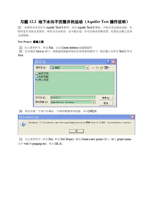
New Project 新建工程[2] 从主菜单栏中，单击File，点击Create database创建数据库[3] 在出现的Save as窗口，将新建的数据库保存在你需要的路径下，然后键入文件名Test12单击Save。

[4] 将会出现一个窗口以确认一个新的数据库的创建，单击[OK]键。

[5] 从主菜单栏中，单击File，单击New Project，弹出Create a new project窗口，键入project name，点中well和pumping test，单击OK键。

[6] 在菜单栏中选中Project点units，单位设置如下图，点OK完成单位的设置并退出改窗口。

Well井[7] 在导航树窗口右击选中Expand all，导航树将全部展开。

[8] 点击New well，然后键入Well name为PW（抽水井），其它参数如下图所示。

然后，在导航树中右击well选择new well另建一观测孔，命名为OW，点OK键。

其它参数如下图所示。

[9] 在绘图区右击，选map→Appearance，可以改变标签的大小及颜色，其设置见下图。

其它设置为默认，点Apply，然后点OK键关闭该窗口。

绘图区将会如下图所示。

Pumping Test 抽水试验[10] 在导航树中点Pumping Test Name，并在Pumping Test Name一栏输入Test12.2，在Saturated aquifer thickness一栏中输入66.70，Performed by一栏输入你的名字，并且可设置时间，在Pumping well一栏中选PW，抽水流量输入1500m3/d。

好的QuickTestProfessional教程QuickT est Professional学习教程，非常好的目录目录 (1)1 QTP 简介 (2)1.1 自动化测试的好处 (2)1.2 QuickTest工作流程 (2)1.3 QTP程序界面 (3)1.4 Mercury T ours 示范网站 (5)2 录制/执行测试脚本 (5)2.1 录制前的准备 (6)2.2 录制测试脚本 (6)2.2.1 录制测试脚本 (6)2.2.2 分析录制的测试脚本 (8)2.3 执行测试脚本 (10)2.3.1 执行脚本出现错误 (11)2.4 分析测试结果 (11)3 建立检查点 (12)3.1 QuickTest检查点种类 (13)3.2 创建检查点 (13)3.2.1 对象检查 (13)3.2.2 网页检查 (16)3.2.3 文字检查 (17)3.2.4 表格检查 (18)3.3 执行并分析使用检查点的测试脚本 (20)4 参数化 (24)4.1 参数化步骤和检查点中的值 (24)4.1.1 参数化对象和检查点的属性值 (24)4.1.2 参数化操作的值 (25)4.2 参数种类 (26)4.2.1 使用数据表参数 (27)4.2.2 使用环境变量参数 (28)4.2.3 使用随机数字参数 (28)4.3 参数化测试脚本 (29)4.3.1 定义参数 (29)4.3.2 修正受到参数化影响的步骤 (30)4.3.3 执行并分析使用参数的测试脚本 (31)5 输出值 (32)5.1 创建输出值 (33)5.1.1 输出值类型 (33)5.1.2 存储输出值 (34)5.2 输出属性值 (35)5.2.1 定义标准输出值 (35)5.2.2 指定输出类型和和设置 (36)5.3 在脚本中建立输出值 (37)5.3.1 建立输出值 (37)5.3.2 执行并分析使用输出值的测试脚本 (40)1QTP 简介1.1 自动化测试的好处如果你执行过人工测试，你一定了解人工测试的缺点，人工测试非常浪费时间而且需要投入大量的人力。

基于水位恢复法的含水层水文地质参数的求解摘要：稳定流抽水试验求取水文地质参数一般要求地下水处于稳定流动状态，由于受各种地质因素的影响，地下水很难保持稳定状态，所以采用传统的方法所预测的水文地质参数精确度并不高。

而水文地质勘测中的水位恢复阶段，由于没有人力和机械因素干扰,其测量数据可以画出平滑的曲线,更适用于水文地质参数的分析。

因此，本文基于水位恢复原理，利用Aquifertest软件中的Theis Recovery对水位恢复数据进行拟合，充分利用停抽后短时间内的恢复水位数据，求出了含水层各种参数，对含水层的贮水性能及释水性能进行了评价。

关键词：水位恢复；水文地质参数；渗透系数；储水系数1绪论在水文地质勘探实践中,一个重要的工作就是确定含水层的水文地质参数[1,2]。

抽水试验则是确定含水层参数的主要途径之一，是以地下水井流理论为基础，通过在井孔中抽水与观测，研究井的涌水量与水位降深的关系及其与抽水延续时间的关系、含水层之间及含水层与地表水体之间的水力联系，求得含水层水文地质参数、评价含水层富水性的一种野外水文地质试验，是获取含水层水文地质参数最有效的手段之一[3]。

水文地质参数，如渗透系数、导水系数、水位传导系数、压力传导系数、给水度、释水系数、越流系数等，是反映含水层或透水层水文地质性能的指标，能为水源井设计或有关水文地质预测提供依据。

而参数精度直接影响井水量计算及地下水资源评价，也为预测井涌水量和评价地下水开采量提供可靠的理论依据[4-7]。

稳定流抽水试验大多采用公式法求参，非稳定流抽水试验采用传统的配线法、直线图解法求参等[8,9]，但这些传统方法人工计算同一井孔抽水试验参数时会因人为误差而得到不同结果，进而直接影响地下水资源的评价结果。

但是利用水位恢复资料求解水文地质参数则可以避免因抽水设备及其它边界条件的干扰因素所造成的不利影响，因此参数的计算结果一般比较可靠。

2“四含”水文地质特征祁南煤矿（隶属于淮北矿业股份有限公司）位于安徽省宿州市埇桥区祁县镇境内，水文地质单元属于南区，矿区范围内无基岩出露，均为松散层覆盖，经钻孔揭露地层有奥陶系、石炭系、二叠系、新近系和第四系。

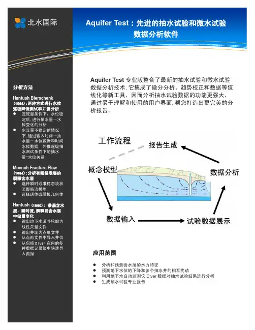
水文地质参数的可视化软件Aquifer Test庞国兴【摘要】Aquifer test是先进的抽水试验和微水试验分析软件,与传统手工计算相比,具有操作简便、实用性强、可视化、对比分析速度快等特点,可大大提高科研人员的工作效率.目前已成位国外比较流行含水层试验分软件,为高效地处理试验数据和参数计算提供帮助,在我国迅速普及推广这套应用软件意义重大.【期刊名称】《地下水》【年(卷),期】2012(000)003【总页数】2页(P195-196)【关键词】Aquifer test;水文地质参数;抽水试验;微水试验;含水层【作者】庞国兴【作者单位】河北省环境地质勘查院,河北石家庄050021【正文语种】中文【中图分类】P642.2含水层的水文地质参数是确定水文地质勘探试验和地下水资源评价中最为重要的研究工作之一，而通过抽水试验可以了解含水层的水力特性和水文地质参数，如导水系数，渗透系数、释水系数、给水度及导压系数等，此目的的抽水试验也被称为含水层试验(Aquifer test)。

近年来，随着计算机技术的发展，求解水文地质参数配线法、直线法等均可借助计算机完成。

目前，由 Waterloo Hydrogeologic.Inc.开发研制的 Aquifer test软件是一款先进的抽水试验与微水试验软件，其主要解决承压水含水层、非承压水含水层、弱透水含水层、基岩裂隙含水层四种情况，主要功能专门用于抽水试验资料的分析、数据处理及求参等，用较短的时间里有效地处理来自含水层试验所有的信息和完成更多的分析。

为水文地质学者和其他水利专家设计提供了方便。

由于Aquifer test软件具有简便、友好、直观的使用界面，并具有优良的可视化效果，目前已成为国际上受欢迎的地下水抽水试验分析软件。

Aquifer test软件系统的硬件运行环境要求并不高，主要包括(1)Pentium系列处理器500 Mhz以上;(2)256 M字节RAM;(3)XGA图形卡和1024x768显示器;(4)使用 windows2000或xp操作系统;(5)硬盘空间75 M字节以上。

AquiferTest软件在抽水试验中的应用AquiferTest软件在抽水试验中的应用引言：地下水是人类生活和工业生产中不可或缺的重要资源。

为了科学、高效地管理和利用地下水资源，地下水抽水试验成为一个必要的环节。

随着计算机技术的发展，各种地下水流动模型和软件工具得到了广泛应用。

其中一款重要的软件工具就是AquiferTest，它被广泛应用于地下水抽水试验的数据分析和模拟过程。

本文将介绍AquiferTest软件的基本原理、应用方法以及其在地下水资源管理中的重要意义。

一、AquiferTest软件的基本原理AquiferTest软件是一款基于单井原理的数值模拟软件，用于分析地下水抽水试验数据。

其基本原理是基于地下水流动方程和井孔流动方程，借助计算机模拟地下水的流动过程。

通过建立适当的数学模型和设定参数，软件能够模拟地下水的压力变化和流量变化，从而对地下水资源进行评估和管理。

二、AquiferTest软件的应用方法使用AquiferTest软件进行抽水试验的数据分析可以分为以下几个步骤：1. 数据导入与测定点设置：首先将实际抽水试验的数据导入软件中，并设置相关的测定点和参数。

2. 地下水模型建立：根据实际情况，通过软件设定适当的地下水模型。

包括选择适合的地下水流动方程、边界条件和初值设定等。

3. 研究参数设置：根据实际需求，设定研究的关键参数，如渗透系数、孔隙度等。

软件将根据这些参数进行模拟计算。

4. 模拟计算与结果分析：软件将根据设定的参数和模型进行模拟计算，并生成模拟结果图表。

根据模拟结果进行数据分析，评估地下水的可持续利用性和资源量。

三、AquiferTest软件在地下水资源管理中的应用意义AquiferTest软件在地下水资源管理中具有重要的应用意义。

首先，在地下水资源评估中，软件能够通过对抽水试验数据的分析，对地下水资源的储量、补给量和消耗量进行准确评估，为科学决策提供依据。

其次，在地下水资源开发与利用中，软件能够通过模拟地下水流动过程，预测地下水位下降速度和补给能力，从而合理规划地下水开采方案，保障地下水资源的可持续利用。

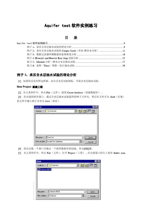
Aquifer test软件实例练习目录Aquifer test软件实例练习 0例子1：承压含水层抽水试验的理论分析 0例子2：承压含水层抽水试验的Cooper-Jacob（库珀-雅各布分析） (11)例子3：数据记录器所测数据的泰斯恢复分析 (16)例子4: Hvorslev and Bouwer-Rice Slug试验分析 (23)练习5：Moench分析—潜水含水层抽水试验 (27)练习6：泰斯（Theis）预报－设计抽水试验 (36)例子1：承压含水层抽水试验的理论分析[1] 如果你还没有照这样做，双击含水层试验图标，开始含水层抽水试验。

New Project 新建工程[2] 从主菜单栏中，单击File（文件），接着Create database（创建数据库）…[3] 在出现的保存窗口，通过含水层抽水试验提供的例子文件夹，然后在文件名为field（区域）的文件中键入例子并单击Save（保存）。

[4] 将会出现一个窗口以确认一个新的数据库的创建，单击[OK]键。

[5] 从主菜单栏中，单击File（文件），打开Project（工程）…在出现窗口的右上角有folder icon（文件夹图标）。

使通过例子文件夹，选择例子。

打开你刚建立的数据库MDB。

[6] 在Open project window（打开工程窗口）中，单击Create Project（创建工程）…[7] 在Create a new project window（创建新工程窗口）中，键入例子，并单击[OK]按钮。

然后，在Open Project window（打开工程窗口）中单击Open（打开）（例子就被突出）。

[8] 在主菜单栏中，单击Project（工程）然后选择Units（单位）。

[9] 对于这个例子，我们将会使用上面显示的单位，如果你的单位不同，相应地进行改变，并单击[OK]按钮。

Well井[10] 在(navigator)（Netscape公司出品的WEB浏览器）面板左边，单击你的鼠标右键，在出现的对话框中选择Expand all（扩大全部）。

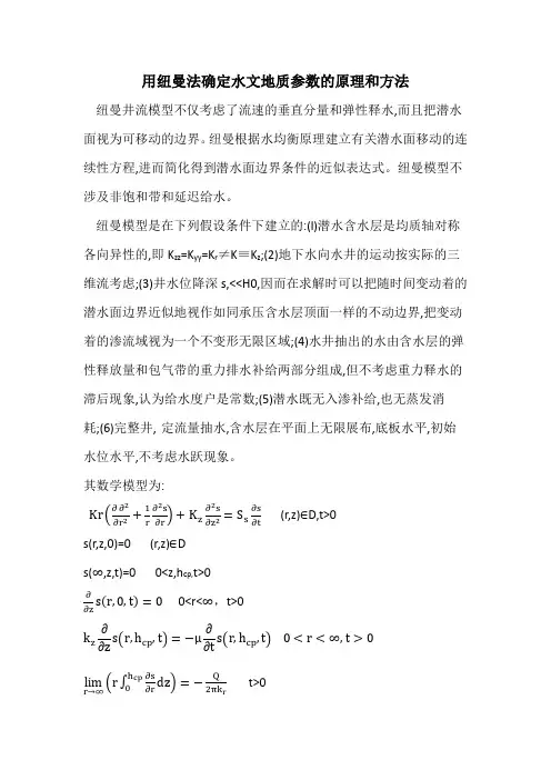
用纽曼法确定水文地质参数的原理和方法纽曼井流模型不仅考虑了流速的垂直分量和弹性释水,而且把潜水面视为可移动的边界。

纽曼根据水均衡原理建立有关潜水面移动的连续性方程,进而简化得到潜水面边界条件的近似表达式。

纽曼模型不涉及非饱和带和延迟给水。

纽曼模型是在下列假设条件下建立的:(l)潜水含水层是均质轴对称各向异性的,即K zz =K yy =K r ≠K ≡K z ;(2)地下水向水井的运动按实际的三维流考虑;(3)井水位降深s,<<H0,因而在求解时可以把随时间变动着的潜水面边界近似地视作如同承压含水层顶面一样的不动边界,把变动着的渗流域视为一个不变形无限区域;(4)水井抽出的水由含水层的弹性释放量和包气带的重力排水补给两部分组成,但不考虑重力释水的滞后现象,认为给水度户是常数;(5)潜水既无入渗补给,也无蒸发消耗;(6)完整井, 定流量抽水,含水层在平面上无限展布,底板水平,初始水位水平,不考虑水跃现象。

其数学模型为:Kr ∂∂2∂r +1r ∂2s ∂r +K z ∂2s ∂z =S s ∂s∂t (r,z)∈D,t>0 s(r,z,0)=0 (r,z)∈Ds(∞,z,t)=0 0<z,h cp,t>0∂∂z s r,0,t =0 0<r<∞，t>0k z ∂s r,h cp ,t =−μ∂s r,h cp ,t 0<r <∞,t >0 lim r →∞ r ∂s ∂r h cp 0dz =−Q2πk r t>0s r,t=Q4πT4yJ0∞yβ1/2w0y+w n y∞n=1dy式中：J0（x）—第一类另零阶贝塞尔函数；β=k zk rrH02;w0y=1−exp−t sβy2−γ02thγ02n nK r—水平径向渗透系数；K z—垂向渗透系数；μs—贮水系数；μ—给水度；H0—潜水流初始厚度；通过对比仿泰斯与纽曼井流模型的假定条件,发现两者的区别在于,纽曼井流模型假定潜水含水介质是轴对称各向异性的。

第３０卷第１０期２　０　１　２年１　０月水　电　能　源　科　学Ｗａｔｅｒ　Ｒｅｓｏｕｒｃｅｓ　ａｎｄ　ＰｏｗｅｒＶｏｌ．３０Ｎｏ．１０Ｏｃｔ．２　０　１　２文章编号：１０００－７７０９（２０１２）１０－００５８－０３ＡｑｕｉｆｅｒＴｅｓｔ软件求解承压含水层水文地质参数的方法及效果陶宗涛，闫志为（桂林理工大学环境科学与工程学院，广西桂林５４１００６）摘要：抽水试验是获取多项水文地质参数最常用的野外水文地质试验方法之一，其参数计算结果精度直接影响地下水资源评价精度。

针对传统水文地质参数计算方法的缺陷，以马楼水源地勘探孔抽水试验为例，采用含水层试验软件ＡｑｕｉｆｅｒＴｅｓｔ计算水文地质参数，并与传统计算方法做了比较。

结果表明，该方法简捷、方便、实用、精度高。

关键词：ＡｑｕｉｆｅｒＴｅｓｔ；水文地质参数；抽水试验；人工求参中图分类号：Ｐ６４１．７３文献标志码：Ａ收稿日期：２０１２－０６－０６，修回日期：２０１２－０７－３１基金项目：广西自然科学基金资助项目（桂科自０９９１２４９）作者简介：陶宗涛（１９８７－），男，硕士研究生，研究方向为水文地质与工程地质，Ｅ－ｍａｉｌ：５０２２６２７４０＠ｑｑ．ｃｏｍ通讯作者：闫志为（１９６３－），男，教授，研究方向为岩溶、水文地球化学与水文地质等，Ｅ－ｍａｉｌ：ｚｈｉｗｅｉｙａｎ＠ｔｏｍ．ｃｏｍ 抽水试验是以地下水井流理论为基础，通过在井孔中抽水与观测，研究井的涌水量与水位降深的关系及其与抽水延续时间的关系、含水层之间及含水层与地表水体之间的水力联系，求得含水层水文地质参数、评价含水层富水性的一种野外水文地质试验，是获取含水层（渗透系数Ｋ、导水系数Ｔ、贮水系数μ＊、给水度μ等）水文地质参数最有效的手段之一。

参数精度直接影响井水量计算及地下水资源评价，也为预测井涌水量和评价地下水开采量提供可靠的理论依据［１］。

稳定流抽水试验大多采用公式法求参，非稳定流抽水试验采用传统的配线法［２］、直线图解法求参等，但这些传统方法人工计算同一井孔抽水试验参数时会因人为误差而得到不同结果［３，４］，进而直接影响地下水资源的评价结果。

安徽焦炭联产甲醇工程一期年产60万吨甲醇项目A1标段抽水试验报告上海设计集团上海工程有限公司二零一一年一月安徽焦炭联产甲醇工程一期年产60万吨甲醇项目A1标段抽水试验报告编写:审核:审定:上海设计集团工程有限公司二零一一年一月二十八日目录第一章前言 (1)第一节工程概况 (1)第二节现场抽水试验 (1)第二章场地地质及水文地质条件 (4)第一节场地地质条件 (4)第二节水文地质条件 (6)第三章单井抽水试验 (6)第一节水文地质钻探 (6)第二节抽水试验 (7)第三节抽水试验观测孔动态 (8)第四节抽水试验参数计算 (10)附件 (15)第四章结论及建议 (17)第一节结论 (17)第二节建议 (17)第一章前言第一节工程概况安徽化工有限公司入驻二坝开发区拟建年产60万吨甲醇项目。

本次拟建为A1区运煤地槽，基坑周长为491m，面积约4519m2。

本基坑开挖深度为自然地面以下6.5～12.7ｍ，已经挖穿承压含水层。

基坑采用三轴搅拌桩止水帷幕，深度为16.6～25.6米，没有隔断承压含水层。

同时本基坑场区内沟塘纵横，场地东南侧为长江，距离本场区较近。

基坑开挖范围内地基土层多为砂性土，含水量特别丰富，且含水层很厚，而基坑开挖又较深，地下水对基坑开挖影响特别大。

鉴于地下水对4#转运站基坑开挖时造成的不利影响，为充分观测和掌握承压水抽水引起对含水层地下水位变化特征、求取水文地质参数、以及降水过程中引起的固结沉降影响，为基坑设计、施工方案制定和优化，有必要在泄煤地槽基坑开挖前做一次有针对性的地下水水文勘察及专项抽水试验。

我公司于2011年1月对该工程进行了水文地质试验，并进行该段工程的地质调查、水文地质调查、钻探、抽水试验等。

根据该地区水文地质条件，进行了两组非稳定流的单井抽水试验，共布置了3个试验井。

第二节现场抽水试验一、目的、任务（一）目的本次试验分为两部分：小流量的单井抽水试验，大流量的单井抽水试验。

AquiferTest Pro v.4.1 Demo Tutorial Advanced Pumping Test & Slug Test Analysis Software©2007, Co-developed by Thomas Röhrich andWaterloo Hydrogeologic, Inc., A Schlumberger CompanyLicense AgreementWaterloo Hydrogeologic Inc., A Schlumberger Company, retains the ownership of this copy of the software. This copy is licensed to you for use under the following conditions:I. Copyright NoticeThis software is protected by both Canadian copyright law and international treaty provisions. Therefore, you must treat this software JUST LIKE A BOOK, with the following single exception. Waterloo Hydrogeologic Inc. authorizes you to make archive copies of the software for the sole purpose of backing-up our software and protecting your investment from loss.By saying “JUST LIKE A BOOK”, Waterloo Hydrogeologic Inc. means, for example, that this software may be used by any number of people and may be freely moved from one computer location to another, so long as there is NO POSSIBILITY of it being used at one location while it is being used at another. Just like a book can't be read by two different people in two different places at the same time.Specifically, you may not distribute, rent, sub-license, or lease the software or documentation; alter, modify, or adapt the software or documentation, including, but not limited to, translating, decompiling, disassembling, or creating derivative works without the prior written consent of Waterloo Hydrogeologic Inc. The provided software and documentation contain trade secrets and it is agreed by the licensee that these trade secrets will not be disclosed to non-licensed persons without written consent of Waterloo Hydrogeologic Inc.II. WarrantyWaterloo Hydrogeologic Inc. warrants that, under normal use, the material on the CD-ROM and the documentation will be free of defects in materials and workmanship for a period of 30 days from the date of purchase. In the event of notification of defects in material or workmanship, Waterloo Hydrogeologic Inc. will replace the CD-ROM or documentation.The remedy for breach of this warranty shall be limited to replacement and shall not encompass any other damages, including but not limited to loss of profit, and special, incidental, consequential, or other similar claims.III. DisclaimerExcept as specifically provided above, neither the developer(s) of this software nor any person or organization acting on behalf of him (them) makes any warranty, express or implied, with respect to this software. In no event will Waterloo Hydrogeologic Inc. assume any liabilities with respect to the use, or misuse, of this software, or the interpretation, or misinterpretation, of any results obtained from this software, or for direct, indirect, special, incidental, or consequential damages resulting from the use of this software.Specifically, Waterloo Hydrogeologic Inc. is not responsible for any costs including, but not limited to, those incurred as a result of lost profits or revenue, loss of use of the computer program, loss of data, the costs of recovering such programs or data, the cost of any substitute program, claims by third parties, or for other similar costs. In no case shall Waterloo Hydrogeologic Inc.'s liability exceed the amount of the license fee. IV. Infringement ProtectionWaterloo Hydrogeologic Inc., A Schlumberger Company, is the sole owner of this software. Waterloo Hydrogeologic Inc. warrants that neither the software and documentation nor any component, including elements provided by others and incorporated into the software and documentation, infringes upon or violates any patent, trademark, copyright, trade secret, or other proprietary right.Royalties or other charges for any patent, trademark, copyright, trade secret or otherproprietary information to be used in the software and documentation shall be considered as included in the contract price.V. Governing LawThis license agreement shall be construed, interpreted, and governed by the laws of the Province of Ontario, Canada, and the United States. Any terms or conditions of this agreement found to be unenforceable, illegal, or contrary to public policy in any jurisdiction will be deleted, but will not affect the remaining terms and conditions of the agreement.VI. Entire AgreementThis agreement constitutes the entire agreement between you and Waterloo Hydrogeologic, Inc., A Schlumberger Company.Table of ContentsIntroduction . . . . . . . . . . . . . . . . . . . . . . . . . . . . . . . . . . . . . . . . . . . 3 Limitations of Demo Version . . . . . . . . . . . . . . . . . . . . . . . . . . . . . . . . . . . . . . . . . . . .3Main Features . . . . . . . . . . . . . . . . . . . . . . . . . . . . . . . . . . . . . . . . . 3 Project Set-up Features . . . . . . . . . . . . . . . . . . . . . . . . . . . . . . . . . . . . . . . . . . . . . . . . .4 Data Entry Features . . . . . . . . . . . . . . . . . . . . . . . . . . . . . . . . . . . . . . . . . . . . . . . . . . .4 Data Analysis Features . . . . . . . . . . . . . . . . . . . . . . . . . . . . . . . . . . . . . . . . . . . . . . . . .4 Graphing and Printing Features . . . . . . . . . . . . . . . . . . . . . . . . . . . . . . . . . . . . . . . . . .5Exercise 1: Confined Aquifer Pumping Test Analysis . . . . . . . . . 5 Project Details . . . . . . . . . . . . . . . . . . . . . . . . . . . . . . . . . . . . . . . . . . . . . . . . . . . . . . . .6 Project Navigator . . . . . . . . . . . . . . . . . . . . . . . . . . . . . . . . . . . . . . . . . . . . . . . . . . . . .6 Project Information . . . . . . . . . . . . . . . . . . . . . . . . . . . . . . . . . . . . . . . . . . . . . . . . . . . .6 Entering Discharge Data . . . . . . . . . . . . . . . . . . . . . . . . . . . . . . . . . . . . . . . . . . . . . . . .7 Entering Water Level Data . . . . . . . . . . . . . . . . . . . . . . . . . . . . . . . . . . . . . . . . . . . . . .8 Creating an Analysis . . . . . . . . . . . . . . . . . . . . . . . . . . . . . . . . . . . . . . . . . . . . . . . . . . .9 Time vs. Drawdown . . . . . . . . . . . . . . . . . . . . . . . . . . . . . . . . . . . . . . . . . . . . . . . . . . . . . . . . . . . . . 9Theis Analysis . . . . . . . . . . . . . . . . . . . . . . . . . . . . . . . . . . . . . . . . . . . . . . . . . . . . . . . . . . . . . . . . 10 Contouring Drawdown . . . . . . . . . . . . . . . . . . . . . . . . . . . . . . . . . . . . . . . . . . . . . . . .18 Determining the effect of the second pumping well . . . . . . . . . . . . . . . . . . . . . . . . . .22 Exercise 2: Predictive Analysis . . . . . . . . . . . . . . . . . . . . . . . . . . . 26 Returning to static level conditions . . . . . . . . . . . . . . . . . . . . . . . . . . . . . . . . . . . . . . . . . . . . . . . . 28 Creating a Report . . . . . . . . . . . . . . . . . . . . . . . . . . . . . . . . . . . . . . . . . . . . . . . . . . . .30Exercise 3: Single Well Analysis . . . . . . . . . . . . . . . . . . . . . . . . . . 31 Interpreting Well Effects with Derivative Analysis . . . . . . . . . . . . . . . . . . . . . . . . . .34 Exercise 4: Slug Test Analysis . . . . . . . . . . . . . . . . . . . . . . . . . . . 36 Hvorslev Analysis . . . . . . . . . . . . . . . . . . . . . . . . . . . . . . . . . . . . . . . . . . . . . . . . . . . .39 Bouwer & Rice Analysis . . . . . . . . . . . . . . . . . . . . . . . . . . . . . . . . . . . . . . . . . . . . . .40 Creating a Report . . . . . . . . . . . . . . . . . . . . . . . . . . . . . . . . . . . . . . . . . . . . . . . . . . . .41IntroductionAquiferTest Pro from Waterloo Hydrogeologic is the latest software technology forgraphical analysis and reporting of pumping and slug test data. This powerful yeteasy-to-use program has everything you need to quickly calculate the hydraulicproperties of your aquifer using a comprehensive selection of pumping and slug testsolution methods for:•Confined aquifers•Unconfined aquifers•Leaky aquifers, and•Fractured rock aquifersIn addition, it is possible to analyze the effects of well interference, and also toaccount for:•Recharge and barrier boundary conditions•Wellbore storage•Partially penetrating pumping and observation wells•Multiple Pumping Wells•Variable pumping rates.AquiferTest Pro can be used as a predictive analysis tool, to calculate water levels /drawdown at any given point based on estimated transmissivity and storativity values.This new functionality allows you to optimize the location of pumping wells,effectively plan your next pumping test.This demo tutorial has been designed to explore many features of AquiferTest Pro,and has been divided into three sections:•Exercise 1: Confined Aquifer Pumping Test Analysis•Exercise 2: Predictive Analysis•Exercise 3: Single Well Analysis•Exercise 4: Slug Test AnalysisLimitations of Demo VersionThe Demo version of AquiferTest is designed to provide you with a brief overview ofthe capabilities of the software. The following limitations exist:•The Save and Save As features have been disabled•Maximum of 20 data points• A watermark “Demo Version” will appear on all print templatesMain FeaturesFor your convenience a description of the main program features has been includedbelow.3Project Set-up Features•Customizable units for length, time, discharge, conductivity, and transmissivity•Import basemaps from common graphic formats (.dxf, .bmp, .wmf., .emf, .jpg)•Display well locations on the basemap•Enter company information and import company logo for printed resultsData Entry Features•Intuitive data entry forms•Cut-and-paste data from Windows clipboard•Import well locations and geometry from a text file•Import and filter data from virtually any datalogger file•Save datalogger import templates (huge time saver!)•Customizable water level datum (top-of-casing, sea level, or benchmark)•On-screen display of water level vs. time graph•Quickly navigate through all data using the Project NavigatorData Analysis FeaturesAquiferTest supports pumping test solutions for the following conditions:•Confined Aquifers•Unconfined Aquifers•Leaky Aquifers•Fracture Flow (Dual Porosity) Aquifers•Fully and partially penetrating Pumping wells and/or Observations wells orPiezometers•Infinite extent of Aquifer or bounded by recharge or barrier boundary•Isotropic or Anisotropic Aquifer•Constant or Variable discharge rates•Single or Multiple pumping wells•Well losses and well storageIn addition, the following analysis tools are available:•Use the Diagnostic Plots to select the appropriate solution method for your aquiferconditions•Select from a comprehensive list of pumping and slug test solution methods forconfined, unconfined, leaky, and fractured rock aquifers and then adjust theassumptions to fit your particular model•Simultaneously analyze data from several different pumping tests•Easily compare and interpret different solution methods for the same data set•Analysis Status Report tells you when data is missing and how to correct the problem•Easily remove selected data from an analysis graph•Fit your data using manual or automatic curve matching (for all data series, or onlyfor selected data in a series)45Graphing and Printing Features•Customize the appearance of the graphs (titles, fonts, lines, axes, symbols, colors, etc.)•Print the map view, tabulated test data, and analysis graphs using professional report layoutsExercise 1: Confined Aquifer Pumping Test AnalysisIf you have not already done so, double-click the AquiferTest Demo icon to start the program. The AquiferTest splash screen will appear followed by a blank project.[1]Select File/Open and browse to the folder AquiferTest\Demo\. [2]Locate the file DemoProject.HYT, and click [Open] and the following windowwill appear:The AquiferTest window is set up so the information can be entered in logicalsuccession from left to right using Navigation tabs .•Pumping Test tab (or Slug test, as the case may be) contains project, test, and aquifer information including units.•Discharge tab (pumping test only) contains discharge data for the pumpingwells.•Water Levels tab contains data for observation wells, pumping wells, andpeizometers used in the selected test. Main menu ToolbarProjectNavigatorWells gridProject informationNavigation tabs•Analysis tab houses all functions needed to perform all analyses available inAquiferTest.•Site Plan tab allows wells to be plotted on a site map, and also contourdrawdown data•Reports tab allows you to tailor the printed report to your specifications.Project DetailsThe pumping test was conducted at Newington Airport, which overlies a 40-foot thicksand and gravel aquifer. There are 3 fully-penetrating wells in the area (Water Supply1, Water Supply 2, and OW-1). Water Supply 1 was pumped at 150 GPM (gallonsper minute) for 24 hours. OW-1 is located 200 feet south of Water Supply 1. WaterSupply 2 will be activated in the second exerciseThe objective of this section is to examine drawdown data from OW-1 and determinethe aquifer transmissivity and storativity. The project basics have already beenestablished including the units and site map (.bmp).Project NavigatorThe project navigator allows you to easily switch between all Array functional parts of AquiferTest.Clicking on any well in their respective frames will take you tothat part of the program where that information is displayed orrequired (i.e. clicking on OW-1 in the Water Levels frame willtake you to the Water Levels tab and activate OW-1 for waterlevel data entry)Two lower frames of the Project Navigator also provide accessto the most frequently used functions of AquiferTest. Fromhere you can access any analysis you have created, create a newanalysis, define time range for the data used in analysis, addcomments to the analysis, import wells from a data file, create anew pumping test, create a new slug test, and contact techsupport.You can hide the Project Navigator by choosing View/Navigation Panel.You can collapse any and all frames in the Project Navigatorby clicking the [-] button beside the header of each frame.Project InformationThe top portion of the Pumping Test tab contains information that describes theproject details, test details, units, and aquifer parameters. Most of the information hasbeen entered for you; however, some additional information is required.6[3]In the Pumping Test frame:•Pumping Test Name: Confined Aquifer Analysis•Performed by: Your Name[4]In the Aquifer Properties frame:•Aquifer Thickness: 40•Type: Confined•Bar. Eff.: leave blankAs mentioned before, the units have been preset in this example, however you caneasily change them using the drop-down menus beside each category and selecting theunit from the provided list.The Convert existing values checkbox allows you to convert the values to the newunits without having to calculate and re-enter them manually.On the other hand if you created a pumping test with incorrect unit labels, you canswitch the labels by de-selecting the Convert existing values option. That way, thephysical labels will change but the numerical values remain the same.Entering Discharge DataNow you need to enter the discharge data for your Water Supply wells.[5]Click on the Discharge tab and activate Water Supply 1 by choosing it fromthe wells list in the top left corner of the form.[6]Select Constant and enter the discharge rate of 150 US gal/min, as shownbelow.For this exercise, the pumping well Water Supply 2 will not be used; this well will be“turned on” in the second exercise, in order to see the effects of multiple pumpingwells.78Entering Water Level DataIn this section, you will import observation water level data from an Excel spreadsheet.AquiferTest can also import data from a datalogger file or a delimited text file, and even paste from the Windows clipboard; this flexibility is important as your pumping test data can be stored in different formats.[7]Click on the Water Levels tab. [8]Select OW-1 from the wells list in the top left corner of the form [9]Enter 4.0 as Static Water Level [10]From the main menu, select File / Import / Water level measurements , or click on the Import button (circled below)[11]In the dialog that appears, browse to the folder AquiferTest\Demo\.[12]Locate the file OW-1.xls file and click [Open]. The Water level measurements will appear in the table. [13]Click on the (Refresh ) button in the toolbar, to refresh the graph. You will see the calculated drawdown data appear in the Drawdown column and a9drawdown graph displayed on the right.Over the 24-hour pumping test, water levels in the observation well dropped almost4.5 feet.Creating an AnalysisIn this section, you will create the analysis graphs, and calculate the aquifer parameters.Time vs. Drawdown[14]Click on the Analysis tab.[15]In the Data from frame, check the box beside OW-1.The first analysis you will perform on the data is the basic Time vs. Drawdown plot.[16]At the top of the Analysis tab, complete the general information about theanalysis as follows:•Analysis name : Time vs. Drawdown•Performed by: your name10•Date: choose current date from the drop-down calendar[17]Select Time-Drawdown from the Analysis Method frame in the AnalysisNavigator.The Time vs. Drawdown analysis appears in the Analyses frame of the Project Navigator.In the next section you will create Theis analysis of your data.Theis Analysis[18]Create a new analysis by selecting Analysis/Create New Analysis or clickingCreate New Analysis in the Analyses frame of the Project Navigator. [19]At the top of the Analysis tab, complete the general information about theanalysis as follows:ProjectNavigatorAnalysisNavigator•Analysis name: Theis•Performed by: your name•Date: choose current date from the drop-down calendarYou will see the Theis analysis name is added to the analyses list in the Analyses frame of the Project Navigator.Theis is the default analysis selected for a pumping test for a confined aquifer. [20]Click the Automatic Fit button above the graph to automatically fit the curve tothe data.Your graph should now look similar to the one shown below.There are numerous graph and display options, such as gridlines, axis intervals,symbol size, and line properties. Feel free to experiment with these options now.1112AquiferTest automatically calculates the Transmissivity and Storativity values and they are displayed in the Results frame of the Analysis Navigator :It is also possible to display the analysis using a dimensionless time drawdown plot (conventional Theis type curve). To see this option, [21]Expand the Display frame under the Analysis Panel (to the right of the main analysis graph).[22]Activate the Dimensionless option, as circled below. [23]Expand the Diagram frame (under the Analysis Panel)13[24]Increase the Marker size to 11.The plot should be displayed similar to the one shown below.AquiferTest has automatically fit the data to the curve, and calculated the aquifer parameters. However the fit includes all the data which is sometimes not the desired case. For example you may wish to place more emphasis on the early time data if you suspect the aquifer is leaky or some other boundary feature is affecting the results.In this pumping test, there is a boundary condition affecting the water levels /drawdown between 700 - 1000 feet south of Water Supply 1. You need to remove the data points after time = 100 minutes.There are several ways to do this, either by de-activating data points in the analysis (they will remain visible but will not be considered in analysis) or by applying a time limit to the data (data outside the time limit is removed from the display). You will examine both options.[25]Return the graph to its original view by setting the following options in the14Analysis Panel:•Display frame•Dimensionless : unchecked•In the Time frame:•Scale: linear •Minimum: 0•Maximum: 2000•Gridlines: unchecked •In the Drawdown frame:•Scale: linear •Minimum: 0•Maximum: 5•Gridlines: unchecked [26]From the main menu, select Analysis / Define Analysis Time Range , or click Define analysis time range in the Analyses frame of the Project Navigator panel The following dialogue will be produced:[27]Select Before and type in 101. This will include all the data-points before 101 minutes and will remove all the data-points after that period. [28]Click [OK] and note that all points after 100 minutes have been temporarily hidden from the graph view.[29]Now, you will modify the graph properties to focus on the early time data.[30]Set the Maximum value for the Time axis to105.15[31]Set the Maximum value for the Drawdown axis to 2.5[32]Click the (Automatic Fit)button above the graph to automatically fit the curve to the data. The points after 100 minutes are no longer visible.With the later points excluded, the calculated parameters in the Results frame have changed to•Transmissivity = 4.48E3 ft2/day•Storativity = 4.27E-4You will now utilize the other method to exclude data points from the graph. First you need to restore the graph to the original view.[33]Select Define analysis time range[34]Choose All and click [OK].[35]You will now exclude the late time data points from the graph. Click the(Exclude) icon above the graph16The following dialogue will be produced:Whereas the Define analysis time range requires you to enter the range in which the data is to be INCLUDED, the Exclude function works the opposite way and requires that you define a time range in which the data will be EXCLUDED. Both perform the similar function, however in different situation one may be more appropriate than the other. Use your discretion for selecting the appropriate method.To define a new period for data exclusion, [36]Type in 101 in the Start field [37]Type 1440 in the End field [38]Click [Add][39]Select and highlight the added period (as shown below), and click [OK][40]Modify the graph properties as follows:•Set the Maximum value for the Time axis to 2000.•Set the Maximum value for the Drawdown axis to5.017[41]Click the (AutomaticFit) button above the graph to automatically fit the curve to the data.Observe, the curve change is identical to the Define analysis time range option (as evident from the calculated parameter values in the Results frame), however the points are still visible.The parameters in the Results frame should now be similar to the following:•Transmissivity = 4.48E3 ft2/day•Storativity = 4.27E-4AquiferTest calculates the best fit line, however that line may not always be ideal. There are two ways in which you can adjust the curve.[42]If you suspect that the aquifer does not conform to the Theis assumptions(confined, infinitely extending, isotropic aquifer), change the assumptions in the Model Assumptions frame of the Analysis Navigator[43]Or, use Parameter Controls to manually adjust the curve fit.18To activate parameter controls, click the parameter controls button above the graph The dialogue shown below allows you to change curve fit, and resulting parameters that are calculated in this analysis.Use the slider-bars to increase or decrease a specific parameter and observe as the relative position of the curve and datapoints change in response. Alternately you can use the up / down arrow keys on your keyboard. You can also simply type in a value in the provided field.[44]Close the Parametersdialog, by clicking on the [X] button in the upper right corner.[45]Restore the best fit parameter values, by clicking on the button.Contouring DrawdownAt this stage it may be advantageous to visualize the drawdown data. You can do so by using the mapping component of AquiferTest located in the Site Plan tab.19[46]Click on the Site Plan tab•Map View - displays the map (if loaded) and the wells from the selected test(s)•Toolbar - provides buttons for map manipulation tools•Well selection - choose the test from which you wish the wells to be displayed •Map properties - provides options for formatting the display properties of themap and contours[47]To obtain a better view of the wells, you may need to zoom out from the defaultmap view. Before displaying contours, you need to select the data series on which the contours will be based.[48]Locate the Data Series field in the Map Properties frame, and click on thebutton in the right portion of that field. The following dialogue will load:[49]Select Theis under the AnalysisframeMap Field Map Properties Well selectiontoolbar20[50]Select OW-1 in the at Well frame [51]Leave the remaining settings, and click [OK][52]In the Map properties , check the box beside Color Shading [53]In the Map properties , check the box beside Contouring Your map display should then be similar to the image shown below You may now modify the color of the color shading and contour lines, following the instructions below.[54]In the Map properties locate the Contour Settings and click on the button in the right portion of that field. The following dialogue will load:[55]In the Contour Linestab, load the color options, and select Black.21[56]For the Interval Distance value, type 0.5[57]For the Minimum value, type 1.5[58]Click [Apply] to apply the changes and update the map view.[59]Click on the Color Shading tab in the Map Appearance dialog, and specify thefollowing settings:•For the Minimum value, type 1.5•For the Maximum value, type 5.0•For the Minimum color, select Blue •For the Maximum color, select Red •For the > color, select the same Red color:[60]Click [OK] to apply the changes and update the map view, and close the Map properties dialogue. The Map window should look similar to the image shownbelow:[61]Before proceeding, turn off the color map and contour lines:•In theMap properties , remove the check mark besideColor Shading•In the Map properties, remove the check mark beside ContouringDetermining the effect of the second pumping wellNow that you have calculated the aquifer parameters, you can use the AquiferTest topredict the effects of applying additional stresses on the aquifer system. In the nextexample, we will activate the second pumping well, and determine what affect thiswill have on the drawdown observed at the observation well.Before proceeding, you must first “lock” the aquifer parameters. Locking theparameters will ensure that the current values for Transmissivity and Storativity willnot be changed when applying the automatic fit.[62]Return to the Analysis tab[63]Select Theis from the Analyses frame of the Project NavigatorLoad the Parameter controls by clicking on the Parameter control icon[64]2223[65]Click the lock icons beside each parameter.[66]Click on the Pumping Test tab[67]In the Wells table, select WaterSupply2 from the well list. To “turn on” thesecond pumping well, change the type from Not Used to Pumping Well[68]Click on the Discharge tab[69]Select WaterSupply2 from the well list[70]Select the Variable discharge option[71]Enter the following pumping rates in the table:TimeDischarge 72015014400These values indicate that the Water Supply 2 well was turned on at the same time as the Water Supply 1, however, whereas Water Supply 1 pumped for 1440 minutes (24 hours) at a constant discharge of 150 US gal/min, Water Supply 2 only ran at thatrate for 720 minutes (12 hours) and was then shut off.。

潜水-微承压含水层水文地质参数求解方法研究任柳妹;杨军耀;吕路【摘要】潜水-微承压含水层水文地质参数是正确评价山西临汾涝洰河生态建设工程,确定水库渗漏量的重要依据.以涝河河谷中段C6典型抽水试验为基础,基于含水层试验(Aquifer Test)专业软件,分析多种方法下获取的潜水-微承压含水层水文地质参数.结果表明,考虑潜水重力释水的Boulton法和水位恢复法求得的水文地质参数稳定可靠,可为后期水文地质数值模拟提供基础数据.%The hydrogeological parameters of phreatic-feeble confined aquifer are important indexes to accurately evaluate LaoJu River Ecological Construction Project in Linfen,Shanxi,and the key basis to confirm reservoir leakage.On the basis of C6 hole pumping test in the middle of Laohe River,the hydrogeological parameters of phreatic-feeble confined aquifer obtained by various methods are analyzed by Aquifer Test software.The result shows that the parameters calculated by the Boulton method which considering phreatic and reliable aquifer gravity water release and the water level recovery method are stable and reliable,which can provide basic data for later hydrogeological numerical simulation.【期刊名称】《水力发电》【年(卷),期】2017(043)003【总页数】7页(P38-43,83)【关键词】水文地质参数;潜水-微承压含水层;含水层试验;Boulton法;涝洰河生态建设工程【作者】任柳妹;杨军耀;吕路【作者单位】太原理工大学水利科学与工程,山西太原030024;太原理工大学水利科学与工程,山西太原030024;太原理工大学水利科学与工程,山西太原030024【正文语种】中文【中图分类】P641.2(225)水文地质参数是水文地质条件中反映含水层或透水层水文地质性能的指标,是进行地下水资源评价、含水层污染风险评价以及地下水数值模拟和溶质运移模拟的前提条件[1],其精确度直接影响后期水文工作。

AquaChem 简要使用说明GAOZANDONG@AquaChem 简要使用说明（编译）--AquaChem是用于水溶液地球化学数据的分析、作图和模拟的专业软件，加拿大滑铁卢水文地质有限公司（Waterloo Hydrogeologic, Inc.）与Lukas Calmbach博士合作开发，前者拥有版权。

--本说明为中国西北地下水开发培训班学员专用。

是在阅读原版用户手册基础上的摘译，并进行重新编排，在省略很多内容的同时对某些操作步骤进行了更为详细地介绍，目的是让计算机操作不很熟练、英语阅读有一定困难的学员对该软件有一个初步了解并能够实际操作。

--如果想深入了解和应用AquaChem软件，请参阅用户手册。

该手册以电子文本方式存储在安装目录下的Tutorials文件夹内，文件名为aqcdemo.pdf。

如果计算机内没有安装打开该文件的Acrobat阅读器，可从互联网上免费下载安装（从任一网站如新浪、搜狐等的搜索引擎上查找以“acrobat”为关键词的“软件”）。

1、简介AquaChem是一个专门用于水溶液地球化学数据的图形和数值分析的软件包。

它具有完全可以由用户自己定制的地球化学数据和参数数据库系统，并提供水文地球化学领域得到广泛应用的多种数据分析和作图工具。

AquaChem的数据分析功能包括单位转换、电荷平衡、样品混合以及样品相关性分析和地球化学参数计算等，辅之以广泛应用的水化学数据图形工具，可以更清楚地表示水的化学特征和质量。

AquaChem的图形工具包括：●三线图，包括piper（图1-1a）、Durov（图1-1b）和简单的三离子三线图（图1-1c）；a，Piper三线图 b，Durov三线图c，三线图图1-1 AquaChem中的三线图a，饼图b，Schoeller指印图c，Stiff折线图 d，放射图图1-2 AquaChem中的饼图、折线图和放射图●饼图（图1-2a）、折线图（Schoeller指印图，图1-2b；Stiff折线图，图1-2c）和放射图（图1-2d）；●散点图，包括一般散点图（图1-3a）和Ludwig-Langelier散点图（图1-3b）；a，一般散点图b，Ludwig-Langelier散点图图1-3 AquaChem中的散点图●频率柱状图（图1-4a）和时间序列图（图1-4b）；a，频率柱状图b，时间序列图图1-4 AquaChem中的频率柱状图和时间序列图●地温图（图1-5）；●样品位置图（图1-6）。