Model selection for support vector machines

Matlab的第三方工具箱大全（强烈推荐）Matlab Toolboxes∙ADCPtools - acoustic doppler current profiler data processing∙AFDesign - designing analog and digital filters∙AIRES - automatic integration of reusable embedded software∙Air-Sea - air-sea flux estimates in oceanography∙Animation - developing scientific animations∙ARfit - estimation of parameters and eigenmodes of multivariate autoregressive methods∙ARMASA - power spectrum estimation∙AR-Toolkit - computer vision tracking∙Auditory - auditory models∙b4m - interval arithmetic∙Bayes Net - inference and learning for directed graphical models∙Binaural Modeling - calculating binaural cross-correlograms of sound∙Bode Step - design of control systems with maximized feedback∙Bootstrap - for resampling, hypothesis testing and confidence interval estimation ∙BrainStorm - MEG and EEG data visualization and processing∙BSTEX - equation viewer∙CALFEM - interactive program for teaching the finite element method∙Calibr - for calibrating CCD cameras∙Camera Calibration∙Captain - non-stationary time series analysis and forecasting∙CHMMBOX - for coupled hidden Markov modeling using maximum likelihood EM∙Classification - supervised and unsupervised classification algorithms∙CLOSID∙Cluster - for analysis of Gaussian mixture models for data set clustering ∙Clustering - cluster analysis∙ClusterPack - cluster analysis∙COLEA - speech analysis∙CompEcon - solving problems in economics and finance∙Complex - for estimating temporal and spatial signal complexities∙Computational Statistics∙Coral - seismic waveform analysis∙DACE - kriging approximations to computer models∙DAIHM - data assimilation in hydrological and hydrodynamic models∙Data Visualization∙DBT - radar array processing∙DDE-BIFTOOL - bifurcation analysis of delay differential equations∙Denoise - for removing noise from signals∙DiffMan - solving differential equations on manifolds∙Dimensional Analysis -∙DIPimage - scientific image processing∙Direct - Laplace transform inversion via the direct integration method ∙DirectSD - analysis and design of computer controlled systems with process-oriented models∙DMsuite - differentiation matrix suite∙DMTTEQ - design and test time domain equalizer design methods∙DrawFilt - drawing digital and analog filters∙DSFWAV - spline interpolation with Dean wave solutions∙DWT - discrete wavelet transforms∙EasyKrig∙Econometrics∙EEGLAB∙EigTool - graphical tool for nonsymmetric eigenproblems∙EMSC - separating light scattering and absorbance by extended multiplicative signal correction∙Engineering Vibration∙FastICA - fixed-point algorithm for ICA and projection pursuit∙FDC - flight dynamics and control∙FDtools - fractional delay filter design∙FlexICA - for independent components analysis∙FMBPC - fuzzy model-based predictive control∙ForWaRD - Fourier-wavelet regularized deconvolution∙FracLab - fractal analysis for signal processing∙FSBOX - stepwise forward and backward selection of features using linear regression∙GABLE - geometric algebra tutorial∙GAOT - genetic algorithm optimization∙Garch - estimating and diagnosing heteroskedasticity in time series models∙GCE Data - managing, analyzing and displaying data and metadata stored using the GCE data structure specification∙GCSV - growing cell structure visualization∙GEMANOVA - fitting multilinear ANOVA models∙Genetic Algorithm∙Geodetic - geodetic calculations∙GHSOM - growing hierarchical self-organizing map∙glmlab - general linear models∙GPIB - wrapper for GPIB library from National Instrument∙GTM - generative topographic mapping, a model for density modeling and data visualization∙GVF - gradient vector flow for finding 3-D object boundaries∙HFRadarmap - converts HF radar data from radial current vectors to total vectors ∙HFRC - importing, processing and manipulating HF radar data∙Hilbert - Hilbert transform by the rational eigenfunction expansion method∙HMM - hidden Markov models∙HMMBOX - for hidden Markov modeling using maximum likelihood EM∙HUTear - auditory modeling∙ICALAB - signal and image processing using ICA and higher order statistics∙Imputation - analysis of incomplete datasets∙IPEM - perception based musical analysisJMatLink - Matlab Java classesKalman - Bayesian Kalman filterKalman Filter - filtering, smoothing and parameter estimation (using EM) for linear dynamical systemsKALMTOOL - state estimation of nonlinear systemsKautz - Kautz filter designKrigingLDestimate - estimation of scaling exponentsLDPC - low density parity check codesLISQ - wavelet lifting scheme on quincunx gridsLKER - Laguerre kernel estimation toolLMAM-OLMAM - Levenberg Marquardt with Adaptive Momentum algorithm for training feedforward neural networksLow-Field NMR - for exponential fitting, phase correction of quadrature data and slicing LPSVM - Newton method for LP support vector machine for machine learning problems LSDPTOOL - robust control system design using the loop shaping design procedureLS-SVMlabLSVM - Lagrangian support vector machine for machine learning problemsLyngby - functional neuroimagingMARBOX - for multivariate autogressive modeling and cross-spectral estimation MatArray - analysis of microarray dataMatrix Computation - constructing test matrices, computing matrix factorizations, visualizing matrices, and direct search optimizationMCAT - Monte Carlo analysisMDP - Markov decision processesMESHPART - graph and mesh partioning methodsMILES - maximum likelihood fitting using ordinary least squares algorithmsMIMO - multidimensional code synthesisMissing - functions for handling missing data valuesM_Map - geographic mapping toolsMODCONS - multi-objective control system designMOEA - multi-objective evolutionary algorithmsMS - estimation of multiscaling exponentsMultiblock - analysis and regression on several data blocks simultaneouslyMultiscale Shape AnalysisMusic Analysis - feature extraction from raw audio signals for content-based music retrievalMWM - multifractal wavelet modelNetCDFNetlab - neural network algorithmsNiDAQ - data acquisition using the NiDAQ libraryNEDM - nonlinear economic dynamic modelsNMM - numerical methods in Matlab textNNCTRL - design and simulation of control systems based on neural networks NNSYSID - neural net based identification of nonlinear dynamic systemsNSVM - newton support vector machine for solving machine learning problems NURBS - non-uniform rational B-splinesN-way - analysis of multiway data with multilinear modelsOpenFEM - finite element developmentPCNN - pulse coupled neural networksPeruna - signal processing and analysisPhiVis - probabilistic hierarchical interactive visualization, i.e. functions for visual analysis of multivariate continuous dataPlanar Manipulator - simulation of n-DOF planar manipulatorsPRTools - pattern recognitionpsignifit - testing hyptheses about psychometric functionsPSVM - proximal support vector machine for solving machine learning problemsPsychophysics - vision researchPyrTools - multi-scale image processingRBF - radial basis function neural networksRBN - simulation of synchronous and asynchronous random boolean networks ReBEL - sigma-point Kalman filtersRegression - basic multivariate data analysis and regressionRegularization ToolsRegularization Tools XPRestore ToolsRobot - robotics functions, e.g. kinematics, dynamics and trajectory generation Robust Calibration - robust calibration in statsRRMT - rainfall-runoff modellingSAM - structure and motionSchwarz-Christoffel - computation of conformal maps to polygonally bounded regions SDH - smoothed data histogramSeaGrid - orthogonal grid makerSEA-MAT - oceanographic analysisSLS - sparse least squaresSolvOpt - solver for local optimization problemsSOM - self-organizing mapSOSTOOLS - solving sums of squares (SOS) optimization problemsSpatial and Geometric AnalysisSpatial RegressionSpatial StatisticsSpectral MethodsSPM - statistical parametric mappingSSVM - smooth support vector machine for solving machine learning problems STATBAG - for linear regression, feature selection, generation of data, and significance testingStatBox - statistical routinesStatistical Pattern Recognition - pattern recognition methodsStixbox - statisticsSVM - implements support vector machinesSVM ClassifierSymbolic Robot DynamicsTEMPLAR - wavelet-based template learning and pattern classificationTextClust - model-based document clusteringTextureSynth - analyzing and synthesizing visual texturesTfMin - continous 3-D minimum time orbit transfer around EarthTime-Frequency - analyzing non-stationary signals using time-frequency distributions Tree-Ring - tasks in tree-ring analysisTSA - uni- and multivariate, stationary and non-stationary time series analysis TSTOOL - nonlinear time series analysisT_Tide - harmonic analysis of tidesUTVtools - computing and modifying rank-revealing URV and UTV decompositionsUvi_Wave - wavelet analysisvarimax - orthogonal rotation of EOFsVBHMM - variation Bayesian hidden Markov modelsVBMFA - variational Bayesian mixtures of factor analyzersVMT - VRML Molecule Toolbox, for animating results from molecular dynamics experiments VOICEBOXVRMLplot - generates interactive VRML 2.0 graphs and animationsVSVtools - computing and modifying symmetric rank-revealing decompositionsWAFO - wave analysis for fatique and oceanographyWarpTB - frequency-warped signal processingWAVEKIT - wavelet analysisWaveLab - wavelet analysisWeeks - Laplace transform inversion via the Weeks methodWetCDF - NetCDF interfaceWHMT - wavelet-domain hidden Markov tree modelsWInHD - Wavelet-based inverse halftoning via deconvolutionWSCT - weighted sequences clustering toolkitXMLTree - XML parserYAADA - analyze single particle mass spectrum dataZMAP - quantitative seismicity analysis。

UNIVERSITY OF SOUTHAMPTONSupport Vector MachinesforClassification and RegressionbySteve R.GunnTechnical ReportFaculty of Engineering,Science and Mathematics School of Electronics and Computer Science10May1998ContentsNomenclature xi1Introduction11.1Statistical Learning Theory (2)1.1.1VC Dimension (3)1.1.2Structural Risk Minimisation (4)2Support Vector Classification52.1The Optimal Separating Hyperplane (5)2.1.1Linearly Separable Example (10)2.2The Generalised Optimal Separating Hyperplane (10)2.2.1Linearly Non-Separable Example (13)2.3Generalisation in High Dimensional Feature Space (14)2.3.1Polynomial Mapping Example (16)2.4Discussion (16)3Feature Space193.1Kernel Functions (19)3.1.1Polynomial (20)3.1.2Gaussian Radial Basis Function (20)3.1.3Exponential Radial Basis Function (20)3.1.4Multi-Layer Perceptron (20)3.1.5Fourier Series (21)3.1.6Splines (21)3.1.7B splines (21)3.1.8Additive Kernels (22)3.1.9Tensor Product (22)3.2Implicit vs.Explicit Bias (22)3.3Data Normalisation (23)3.4Kernel Selection (23)4Classification Example:IRIS data254.1Applications (28)5Support Vector Regression295.1Linear Regression (30)5.1.1 -insensitive Loss Function (30)5.1.2Quadratic Loss Function (31)iiiiv CONTENTS5.1.3Huber Loss Function (32)5.1.4Example (33)5.2Non Linear Regression (33)5.2.1Examples (34)5.2.2Comments (36)6Regression Example:Titanium Data396.1Applications (42)7Conclusions43A Implementation Issues45A.1Support Vector Classification (45)A.2Support Vector Regression (47)B MATLAB SVM Toolbox51 Bibliography53List of Figures1.1Modelling Errors (2)1.2VC Dimension Illustration (3)2.1Optimal Separating Hyperplane (5)2.2Canonical Hyperplanes (6)2.3Constraining the Canonical Hyperplanes (7)2.4Optimal Separating Hyperplane (10)2.5Generalised Optimal Separating Hyperplane (11)2.6Generalised Optimal Separating Hyperplane Example(C=1) (13)2.7Generalised Optimal Separating Hyperplane Example(C=105) (14)2.8Generalised Optimal Separating Hyperplane Example(C=10−8) (14)2.9Mapping the Input Space into a High Dimensional Feature Space (14)2.10Mapping input space into Polynomial Feature Space (16)3.1Comparison between Implicit and Explicit bias for a linear kernel (22)4.1Iris data set (25)4.2Separating Setosa with a linear SVC(C=∞) (26)4.3Separating Viginica with a polynomial SVM(degree2,C=∞) (26)4.4Separating Viginica with a polynomial SVM(degree10,C=∞) (26)4.5Separating Viginica with a Radial Basis Function SVM(σ=1.0,C=∞)274.6Separating Viginica with a polynomial SVM(degree2,C=10) (27)4.7The effect of C on the separation of Versilcolor with a linear spline SVM.285.1Loss Functions (29)5.2Linear regression (33)5.3Polynomial Regression (35)5.4Radial Basis Function Regression (35)5.5Spline Regression (36)5.6B-spline Regression (36)5.7Exponential RBF Regression (36)6.1Titanium Linear Spline Regression( =0.05,C=∞) (39)6.2Titanium B-Spline Regression( =0.05,C=∞) (40)6.3Titanium Gaussian RBF Regression( =0.05,σ=1.0,C=∞) (40)6.4Titanium Gaussian RBF Regression( =0.05,σ=0.3,C=∞) (40)6.5Titanium Exponential RBF Regression( =0.05,σ=1.0,C=∞) (41)6.6Titanium Fourier Regression( =0.05,degree3,C=∞) (41)6.7Titanium Linear Spline Regression( =0.05,C=10) (42)vvi LIST OF FIGURES6.8Titanium B-Spline Regression( =0.05,C=10) (42)List of Tables2.1Linearly Separable Classification Data (10)2.2Non-Linearly Separable Classification Data (13)5.1Regression Data (33)viiListingsA.1Support Vector Classification MATLAB Code (46)A.2Support Vector Regression MATLAB Code (48)ixNomenclature0Column vector of zeros(x)+The positive part of xC SVM misclassification tolerance parameterD DatasetK(x,x )Kernel functionR[f]Risk functionalR emp[f]Empirical Risk functionalxiChapter1IntroductionThe problem of empirical data modelling is germane to many engineering applications. In empirical data modelling a process of induction is used to build up a model of the system,from which it is hoped to deduce responses of the system that have yet to be ob-served.Ultimately the quantity and quality of the observations govern the performance of this empirical model.By its observational nature data obtained isfinite and sampled; typically this sampling is non-uniform and due to the high dimensional nature of the problem the data will form only a sparse distribution in the input space.Consequently the problem is nearly always ill posed(Poggio et al.,1985)in the sense of Hadamard (Hadamard,1923).Traditional neural network approaches have suffered difficulties with generalisation,producing models that can overfit the data.This is a consequence of the optimisation algorithms used for parameter selection and the statistical measures used to select the’best’model.The foundations of Support Vector Machines(SVM)have been developed by Vapnik(1995)and are gaining popularity due to many attractive features,and promising empirical performance.The formulation embodies the Struc-tural Risk Minimisation(SRM)principle,which has been shown to be superior,(Gunn et al.,1997),to traditional Empirical Risk Minimisation(ERM)principle,employed by conventional neural networks.SRM minimises an upper bound on the expected risk, as opposed to ERM that minimises the error on the training data.It is this difference which equips SVM with a greater ability to generalise,which is the goal in statistical learning.SVMs were developed to solve the classification problem,but recently they have been extended to the domain of regression problems(Vapnik et al.,1997).In the literature the terminology for SVMs can be slightly confusing.The term SVM is typ-ically used to describe classification with support vector methods and support vector regression is used to describe regression with support vector methods.In this report the term SVM will refer to both classification and regression methods,and the terms Support Vector Classification(SVC)and Support Vector Regression(SVR)will be used for specification.This section continues with a brief introduction to the structural risk12Chapter1Introductionminimisation principle.In Chapter2the SVM is introduced in the setting of classifica-tion,being both historical and more accessible.This leads onto mapping the input into a higher dimensional feature space by a suitable choice of kernel function.The report then considers the problem of regression.Illustrative examples re given to show the properties of the techniques.1.1Statistical Learning TheoryThis section is a very brief introduction to statistical learning theory.For a much more in depth look at statistical learning theory,see(Vapnik,1998).Figure1.1:Modelling ErrorsThe goal in modelling is to choose a model from the hypothesis space,which is closest (with respect to some error measure)to the underlying function in the target space. Errors in doing this arise from two cases:Approximation Error is a consequence of the hypothesis space being smaller than the target space,and hence the underlying function may lie outside the hypothesis space.A poor choice of the model space will result in a large approximation error, and is referred to as model mismatch.Estimation Error is the error due to the learning procedure which results in a tech-nique selecting the non-optimal model from the hypothesis space.Chapter1Introduction3Together these errors form the generalisation error.Ultimately we would like tofind the function,f,which minimises the risk,R[f]=X×YL(y,f(x))P(x,y)dxdy(1.1)However,P(x,y)is unknown.It is possible tofind an approximation according to the empirical risk minimisation principle,R emp[f]=1lli=1Ly i,fx i(1.2)which minimises the empirical risk,ˆf n,l (x)=arg minf∈H nR emp[f](1.3)Empirical risk minimisation makes sense only if,liml→∞R emp[f]=R[f](1.4) which is true from the law of large numbers.However,it must also satisfy,lim l→∞minf∈H nR emp[f]=minf∈H nR[f](1.5)which is only valid when H n is’small’enough.This condition is less intuitive and requires that the minima also converge.The following bound holds with probability1−δ,R[f]≤R emp[f]+h ln2lh+1−lnδ4l(1.6)Remarkably,this expression for the expected risk is independent of the probability dis-tribution.1.1.1VC DimensionThe VC dimension is a scalar value that measures the capacity of a set offunctions.Figure1.2:VC Dimension Illustration4Chapter1IntroductionDefinition1.1(Vapnik–Chervonenkis).The VC dimension of a set of functions is p if and only if there exists a set of points{x i}pi=1such that these points can be separatedin all2p possible configurations,and that no set{x i}qi=1exists where q>p satisfying this property.Figure1.2illustrates how three points in the plane can be shattered by the set of linear indicator functions whereas four points cannot.In this case the VC dimension is equal to the number of free parameters,but in general that is not the case;e.g.the function A sin(bx)has an infinite VC dimension(Vapnik,1995).The set of linear indicator functions in n dimensional space has a VC dimension equal to n+1.1.1.2Structural Risk MinimisationCreate a structure such that S h is a hypothesis space of VC dimension h then,S1⊂S2⊂...⊂S∞(1.7) SRM consists in solving the following problemmin S h R emp[f]+h ln2lh+1−lnδ4l(1.8)If the underlying process being modelled is not deterministic the modelling problem becomes more exacting and consequently this chapter is restricted to deterministic pro-cesses.Multiple output problems can usually be reduced to a set of single output prob-lems that may be considered independent.Hence it is appropriate to consider processes with multiple inputs from which it is desired to predict a single output.Chapter2Support Vector ClassificationThe classification problem can be restricted to consideration of the two-class problem without loss of generality.In this problem the goal is to separate the two classes by a function which is induced from available examples.The goal is to produce a classifier that will work well on unseen examples,i.e.it generalises well.Consider the example in Figure2.1.Here there are many possible linear classifiers that can separate the data, but there is only one that maximises the margin(maximises the distance between it and the nearest data point of each class).This linear classifier is termed the optimal separating hyperplane.Intuitively,we would expect this boundary to generalise well as opposed to the other possible boundaries.Figure2.1:Optimal Separating Hyperplane2.1The Optimal Separating HyperplaneConsider the problem of separating the set of training vectors belonging to two separateclasses,D=(x1,y1),...,(x l,y l),x∈R n,y∈{−1,1},(2.1)56Chapter 2Support Vector Classificationwith a hyperplane, w,x +b =0.(2.2)The set of vectors is said to be optimally separated by the hyperplane if it is separated without error and the distance between the closest vector to the hyperplane is maximal.There is some redundancy in Equation 2.2,and without loss of generality it is appropri-ate to consider a canonical hyperplane (Vapnik ,1995),where the parameters w ,b are constrained by,min i w,x i +b =1.(2.3)This incisive constraint on the parameterisation is preferable to alternatives in simpli-fying the formulation of the problem.In words it states that:the norm of the weight vector should be equal to the inverse of the distance,of the nearest point in the data set to the hyperplane .The idea is illustrated in Figure 2.2,where the distance from the nearest point to each hyperplane is shown.Figure 2.2:Canonical HyperplanesA separating hyperplane in canonical form must satisfy the following constraints,y i w,x i +b ≥1,i =1,...,l.(2.4)The distance d (w,b ;x )of a point x from the hyperplane (w,b )is,d (w,b ;x )= w,x i +bw .(2.5)Chapter 2Support Vector Classification 7The optimal hyperplane is given by maximising the margin,ρ,subject to the constraints of Equation 2.4.The margin is given by,ρ(w,b )=min x i :y i =−1d (w,b ;x i )+min x i :y i =1d (w,b ;x i )=min x i :y i =−1 w,x i +b w +min x i :y i =1 w,x i +b w =1 w min x i :y i =−1 w,x i +b +min x i :y i =1w,x i +b =2 w (2.6)Hence the hyperplane that optimally separates the data is the one that minimisesΦ(w )=12 w 2.(2.7)It is independent of b because provided Equation 2.4is satisfied (i.e.it is a separating hyperplane)changing b will move it in the normal direction to itself.Accordingly the margin remains unchanged but the hyperplane is no longer optimal in that it will be nearer to one class than the other.To consider how minimising Equation 2.7is equivalent to implementing the SRM principle,suppose that the following bound holds,w <A.(2.8)Then from Equation 2.4and 2.5,d (w,b ;x )≥1A.(2.9)Accordingly the hyperplanes cannot be nearer than 1A to any of the data points and intuitively it can be seen in Figure 2.3how this reduces the possible hyperplanes,andhence thecapacity.Figure 2.3:Constraining the Canonical Hyperplanes8Chapter2Support Vector ClassificationThe VC dimension,h,of the set of canonical hyperplanes in n dimensional space is bounded by,h≤min[R2A2,n]+1,(2.10)where R is the radius of a hypersphere enclosing all the data points.Hence minimising Equation2.7is equivalent to minimising an upper bound on the VC dimension.The solution to the optimisation problem of Equation2.7under the constraints of Equation 2.4is given by the saddle point of the Lagrange functional(Lagrangian)(Minoux,1986),Φ(w,b,α)=12 w 2−li=1αiy iw,x i +b−1,(2.11)whereαare the Lagrange multipliers.The Lagrangian has to be minimised with respect to w,b and maximised with respect toα≥0.Classical Lagrangian duality enables the primal problem,Equation2.11,to be transformed to its dual problem,which is easier to solve.The dual problem is given by,max αW(α)=maxαminw,bΦ(w,b,α).(2.12)The minimum with respect to w and b of the Lagrangian,Φ,is given by,∂Φ∂b =0⇒li=1αi y i=0∂Φ∂w =0⇒w=li=1αi y i x i.(2.13)Hence from Equations2.11,2.12and2.13,the dual problem is,max αW(α)=maxα−12li=1lj=1αiαj y i y j x i,x j +lk=1αk,(2.14)and hence the solution to the problem is given by,α∗=arg minα12li=1lj=1αiαj y i y j x i,x j −lk=1αk,(2.15)with constraints,αi≥0i=1,...,llj=1αj y j=0.(2.16)Chapter2Support Vector Classification9Solving Equation2.15with constraints Equation2.16determines the Lagrange multi-pliers,and the optimal separating hyperplane is given by,w∗=li=1αi y i x ib∗=−12w∗,x r+x s .(2.17)where x r and x s are any support vector from each class satisfying,αr,αs>0,y r=−1,y s=1.(2.18)The hard classifier is then,f(x)=sgn( w∗,x +b)(2.19) Alternatively,a soft classifier may be used which linearly interpolates the margin,f(x)=h( w∗,x +b)where h(z)=−1:z<−1z:−1≤z≤1+1:z>1(2.20)This may be more appropriate than the hard classifier of Equation2.19,because it produces a real valued output between−1and1when the classifier is queried within the margin,where no training data resides.From the Kuhn-Tucker conditions,αiy iw,x i +b−1=0,i=1,...,l,(2.21)and hence only the points x i which satisfy,y iw,x i +b=1(2.22)will have non-zero Lagrange multipliers.These points are termed Support Vectors(SV). If the data is linearly separable all the SV will lie on the margin and hence the number of SV can be very small.Consequently the hyperplane is determined by a small subset of the training set;the other points could be removed from the training set and recalculating the hyperplane would produce the same answer.Hence SVM can be used to summarise the information contained in a data set by the SV produced.If the data is linearly separable the following equality will hold,w 2=li=1αi=i∈SV sαi=i∈SV sj∈SV sαiαj y i y j x i,x j .(2.23)Hence from Equation2.10the VC dimension of the classifier is bounded by,h≤min[R2i∈SV s,n]+1,(2.24)10Chapter2Support Vector Classificationx1x2y11-133113131-12 2.513 2.5-143-1Table2.1:Linearly Separable Classification Dataand if the training data,x,is normalised to lie in the unit hypersphere,,n],(2.25)h≤1+min[i∈SV s2.1.1Linearly Separable ExampleTo illustrate the method consider the training set in Table2.1.The SVC solution is shown in Figure2.4,where the dotted lines describe the locus of the margin and the circled data points represent the SV,which all lie on the margin.Figure2.4:Optimal Separating Hyperplane2.2The Generalised Optimal Separating HyperplaneSo far the discussion has been restricted to the case where the training data is linearly separable.However,in general this will not be the case,Figure2.5.There are two approaches to generalising the problem,which are dependent upon prior knowledge of the problem and an estimate of the noise on the data.In the case where it is expected (or possibly even known)that a hyperplane can correctly separate the data,a method ofChapter2Support Vector Classification11Figure2.5:Generalised Optimal Separating Hyperplaneintroducing an additional cost function associated with misclassification is appropriate. Alternatively a more complex function can be used to describe the boundary,as discussed in Chapter2.1.To enable the optimal separating hyperplane method to be generalised, Cortes and Vapnik(1995)introduced non-negative variables,ξi≥0,and a penalty function,Fσ(ξ)=iξσiσ>0,(2.26) where theξi are a measure of the misclassification errors.The optimisation problem is now posed so as to minimise the classification error as well as minimising the bound on the VC dimension of the classifier.The constraints of Equation2.4are modified for the non-separable case to,y iw,x i +b≥1−ξi,i=1,...,l.(2.27)whereξi≥0.The generalised optimal separating hyperplane is determined by the vector w,that minimises the functional,Φ(w,ξ)=12w 2+Ciξi,(2.28)(where C is a given value)subject to the constraints of Equation2.27.The solution to the optimisation problem of Equation2.28under the constraints of Equation2.27is given by the saddle point of the Lagrangian(Minoux,1986),Φ(w,b,α,ξ,β)=12 w 2+Ciξi−li=1αiy iw T x i+b−1+ξi−lj=1βiξi,(2.29)12Chapter2Support Vector Classificationwhereα,βare the Lagrange multipliers.The Lagrangian has to be minimised with respect to w,b,x and maximised with respect toα,β.As before,classical Lagrangian duality enables the primal problem,Equation2.29,to be transformed to its dual problem. The dual problem is given by,max αW(α,β)=maxα,βminw,b,ξΦ(w,b,α,ξ,β).(2.30)The minimum with respect to w,b andξof the Lagrangian,Φ,is given by,∂Φ∂b =0⇒li=1αi y i=0∂Φ∂w =0⇒w=li=1αi y i x i∂Φ∂ξ=0⇒αi+βi=C.(2.31) Hence from Equations2.29,2.30and2.31,the dual problem is,max αW(α)=maxα−12li=1lj=1αiαj y i y j x i,x j +lk=1αk,(2.32)and hence the solution to the problem is given by,α∗=arg minα12li=1lj=1αiαj y i y j x i,x j −lk=1αk,(2.33)with constraints,0≤αi≤C i=1,...,llj=1αj y j=0.(2.34)The solution to this minimisation problem is identical to the separable case except for a modification of the bounds of the Lagrange multipliers.The uncertain part of Cortes’s approach is that the coefficient C has to be determined.This parameter introduces additional capacity control within the classifier.C can be directly related to a regulari-sation parameter(Girosi,1997;Smola and Sch¨o lkopf,1998).Blanz et al.(1996)uses a value of C=5,but ultimately C must be chosen to reflect the knowledge of the noise on the data.This warrants further work,but a more practical discussion is given in Chapter4.Chapter2Support Vector Classification13x1x2y11-133113131-12 2.513 2.5-143-11.5 1.5112-1Table2.2:Non-Linearly Separable Classification Data2.2.1Linearly Non-Separable ExampleTwo additional data points are added to the separable data of Table2.1to produce a linearly non-separable data set,Table2.2.The resulting SVC is shown in Figure2.6,for C=1.The SV are no longer required to lie on the margin,as in Figure2.4,and the orientation of the hyperplane and the width of the margin are different.Figure2.6:Generalised Optimal Separating Hyperplane Example(C=1)In the limit,lim C→∞the solution converges towards the solution obtained by the optimal separating hyperplane(on this non-separable data),Figure2.7.In the limit,lim C→0the solution converges to one where the margin maximisation term dominates,Figure2.8.Beyond a certain point the Lagrange multipliers will all take on the value of C.There is now less emphasis on minimising the misclassification error, but purely on maximising the margin,producing a large width margin.Consequently as C decreases the width of the margin increases.The useful range of C lies between the point where all the Lagrange Multipliers are equal to C and when only one of them is just bounded by C.14Chapter2Support Vector ClassificationFigure2.7:Generalised Optimal Separating Hyperplane Example(C=105)Figure2.8:Generalised Optimal Separating Hyperplane Example(C=10−8)2.3Generalisation in High Dimensional Feature SpaceIn the case where a linear boundary is inappropriate the SVM can map the input vector, x,into a high dimensional feature space,z.By choosing a non-linear mapping a priori, the SVM constructs an optimal separating hyperplane in this higher dimensional space, Figure2.9.The idea exploits the method of Aizerman et al.(1964)which,enables the curse of dimensionality(Bellman,1961)to be addressed.Figure2.9:Mapping the Input Space into a High Dimensional Feature SpaceChapter2Support Vector Classification15There are some restrictions on the non-linear mapping that can be employed,see Chap-ter3,but it turns out,surprisingly,that most commonly employed functions are accept-able.Among acceptable mappings are polynomials,radial basis functions and certain sigmoid functions.The optimisation problem of Equation2.33becomes,α∗=arg minα12li=1lj=1αiαj y i y j K(x i,x j)−lk=1αk,(2.35)where K(x,x )is the kernel function performing the non-linear mapping into feature space,and the constraints are unchanged,0≤αi≤C i=1,...,llj=1αj y j=0.(2.36)Solving Equation2.35with constraints Equation2.36determines the Lagrange multipli-ers,and a hard classifier implementing the optimal separating hyperplane in the feature space is given by,f(x)=sgn(i∈SV sαi y i K(x i,x)+b)(2.37) wherew∗,x =li=1αi y i K(x i,x)b∗=−12li=1αi y i[K(x i,x r)+K(x i,x r)].(2.38)The bias is computed here using two support vectors,but can be computed using all the SV on the margin for stability(Vapnik et al.,1997).If the Kernel contains a bias term, the bias can be accommodated within the Kernel,and hence the classifier is simply,f(x)=sgn(i∈SV sαi K(x i,x))(2.39)Many employed kernels have a bias term and anyfinite Kernel can be made to have one(Girosi,1997).This simplifies the optimisation problem by removing the equality constraint of Equation2.36.Chapter3discusses the necessary conditions that must be satisfied by valid kernel functions.16Chapter2Support Vector Classification 2.3.1Polynomial Mapping ExampleConsider a polynomial kernel of the form,K(x,x )=( x,x +1)2,(2.40)which maps a two dimensional input vector into a six dimensional feature space.Apply-ing the non-linear SVC to the linearly non-separable training data of Table2.2,produces the classification illustrated in Figure2.10(C=∞).The margin is no longer of constant width due to the non-linear projection into the input space.The solution is in contrast to Figure2.7,in that the training data is now classified correctly.However,even though SVMs implement the SRM principle and hence can generalise well,a careful choice of the kernel function is necessary to produce a classification boundary that is topologically appropriate.It is always possible to map the input space into a dimension greater than the number of training points and produce a classifier with no classification errors on the training set.However,this will generalise badly.Figure2.10:Mapping input space into Polynomial Feature Space2.4DiscussionTypically the data will only be linearly separable in some,possibly very high dimensional feature space.It may not make sense to try and separate the data exactly,particularly when only afinite amount of training data is available which is potentially corrupted by noise.Hence in practice it will be necessary to employ the non-separable approach which places an upper bound on the Lagrange multipliers.This raises the question of how to determine the parameter C.It is similar to the problem in regularisation where the regularisation coefficient has to be determined,and it has been shown that the parameter C can be directly related to a regularisation parameter for certain kernels (Smola and Sch¨o lkopf,1998).A process of cross-validation can be used to determine thisChapter2Support Vector Classification17parameter,although more efficient and potentially better methods are sought after.In removing the training patterns that are not support vectors,the solution is unchanged and hence a fast method for validation may be available when the support vectors are sparse.Chapter3Feature SpaceThis chapter discusses the method that can be used to construct a mapping into a high dimensional feature space by the use of reproducing kernels.The idea of the kernel function is to enable operations to be performed in the input space rather than the potentially high dimensional feature space.Hence the inner product does not need to be evaluated in the feature space.This provides a way of addressing the curse of dimensionality.However,the computation is still critically dependent upon the number of training patterns and to provide a good data distribution for a high dimensional problem will generally require a large training set.3.1Kernel FunctionsThe following theory is based upon Reproducing Kernel Hilbert Spaces(RKHS)(Aron-szajn,1950;Girosi,1997;Heckman,1997;Wahba,1990).An inner product in feature space has an equivalent kernel in input space,K(x,x )= φ(x),φ(x ) ,(3.1)provided certain conditions hold.If K is a symmetric positive definite function,which satisfies Mercer’s Conditions,K(x,x )=∞ma mφm(x)φm(x ),a m≥0,(3.2)K(x,x )g(x)g(x )dxdx >0,g∈L2,(3.3) then the kernel represents a legitimate inner product in feature space.Valid functions that satisfy Mercer’s conditions are now given,which unless stated are valid for all real x and x .1920Chapter3Feature Space3.1.1PolynomialA polynomial mapping is a popular method for non-linear modelling,K(x,x )= x,x d.(3.4)K(x,x )=x,x +1d.(3.5)The second kernel is usually preferable as it avoids problems with the hessian becoming zero.3.1.2Gaussian Radial Basis FunctionRadial basis functions have received significant attention,most commonly with a Gaus-sian of the form,K(x,x )=exp−x−x 22σ2.(3.6)Classical techniques utilising radial basis functions employ some method of determining a subset of centres.Typically a method of clustering isfirst employed to select a subset of centres.An attractive feature of the SVM is that this selection is implicit,with each support vectors contributing one local Gaussian function,centred at that data point. By further considerations it is possible to select the global basis function width,s,using the SRM principle(Vapnik,1995).3.1.3Exponential Radial Basis FunctionA radial basis function of the form,K(x,x )=exp−x−x2σ2.(3.7)produces a piecewise linear solution which can be attractive when discontinuities are acceptable.3.1.4Multi-Layer PerceptronThe long established MLP,with a single hidden layer,also has a valid kernel represen-tation,K(x,x )=tanhρ x,x +(3.8)for certain values of the scale,ρ,and offset, ,parameters.Here the SV correspond to thefirst layer and the Lagrange multipliers to the weights.。

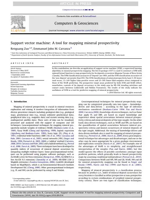
Support vector machine:A tool for mapping mineral prospectivityRenguang Zuo a,n,Emmanuel John M.Carranza ba State Key Laboratory of Geological Processes and Mineral Resources,China University of Geosciences,Wuhan430074;Beijing100083,Chinab Department of Earth Systems Analysis,Faculty of Geo-Information Science and Earth Observation(ITC),University of Twente,Enschede,The Netherlandsa r t i c l e i n f oArticle history:Received17May2010Received in revised form3September2010Accepted25September2010Keywords:Supervised learning algorithmsKernel functionsWeights-of-evidenceTurbidite-hosted AuMeguma Terraina b s t r a c tIn this contribution,we describe an application of support vector machine(SVM),a supervised learningalgorithm,to mineral prospectivity mapping.The free R package e1071is used to construct a SVM withsigmoid kernel function to map prospectivity for Au deposits in western Meguma Terrain of Nova Scotia(Canada).The SVM classification accuracies of‘deposit’are100%,and the SVM classification accuracies ofthe‘non-deposit’are greater than85%.The SVM classifications of mineral prospectivity have5–9%lowertotal errors,13–14%higher false-positive errors and25–30%lower false-negative errors compared tothose of the WofE prediction.The prospective target areas predicted by both SVM and WofE reflect,nonetheless,controls of Au deposit occurrence in the study area by NE–SW trending anticlines andcontact zones between Goldenville and Halifax Formations.The results of the study indicate theusefulness of SVM as a tool for predictive mapping of mineral prospectivity.&2010Elsevier Ltd.All rights reserved.1.IntroductionMapping of mineral prospectivity is crucial in mineral resourcesexploration and mining.It involves integration of information fromdiverse geoscience datasets including geological data(e.g.,geologicalmap),geochemical data(e.g.,stream sediment geochemical data),geophysical data(e.g.,magnetic data)and remote sensing data(e.g.,multispectral satellite data).These sorts of data can be visualized,processed and analyzed with the support of computer and GIStechniques.Geocomputational techniques for mapping mineral pro-spectivity include weights of evidence(WofE)(Bonham-Carter et al.,1989),fuzzy WofE(Cheng and Agterberg,1999),logistic regression(Agterberg and Bonham-Carter,1999),fuzzy logic(FL)(Ping et al.,1991),evidential belief functions(EBF)(An et al.,1992;Carranza andHale,2003;Carranza et al.,2005),neural networks(NN)(Singer andKouda,1996;Porwal et al.,2003,2004),a‘wildcat’method(Carranza,2008,2010;Carranza and Hale,2002)and a hybrid method(e.g.,Porwalet al.,2006;Zuo et al.,2009).These techniques have been developed toquantify indices of occurrence of mineral deposit occurrence byintegrating multiple evidence layers.Some geocomputational techni-ques can be performed using popular software packages,such asArcWofE(a free ArcView extension)(Kemp et al.,1999),ArcSDM9.3(afree ArcGIS9.3extension)(Sawatzky et al.,2009),MI-SDM2.50(aMapInfo extension)(Avantra Geosystems,2006),GeoDAS(developedbased on MapObjects,which is an Environmental Research InstituteDevelopment Kit)(Cheng,2000).Other geocomputational techniques(e.g.,FL and NN)can be performed by using R and Matlab.Geocomputational techniques for mineral prospectivity map-ping can be categorized generally into two types–knowledge-driven and data-driven–according to the type of inferencemechanism considered(Bonham-Carter1994;Pan and Harris2000;Carranza2008).Knowledge-driven techniques,such as thosethat apply FL and EBF,are based on expert knowledge andexperience about spatial associations between mineral prospec-tivity criteria and mineral deposits of the type sought.On the otherhand,data-driven techniques,such as WofE and NN,are based onthe quantification of spatial associations between mineral pro-spectivity criteria and known occurrences of mineral deposits ofthe type sought.Additional,the mixing of knowledge-driven anddata-driven methods also is used for mapping of mineral prospec-tivity(e.g.,Porwal et al.,2006;Zuo et al.,2009).Every geocomputa-tional technique has advantages and disadvantages,and one or theother may be more appropriate for a given geologic environmentand exploration scenario(Harris et al.,2001).For example,one ofthe advantages of WofE is its simplicity,and straightforwardinterpretation of the weights(Pan and Harris,2000),but thismodel ignores the effects of possible correlations amongst inputpredictor patterns,which generally leads to biased prospectivitymaps by assuming conditional independence(Porwal et al.,2010).Comparisons between WofE and NN,NN and LR,WofE,NN and LRfor mineral prospectivity mapping can be found in Singer andKouda(1999),Harris and Pan(1999)and Harris et al.(2003),respectively.Mapping of mineral prospectivity is a classification process,because its product(i.e.,index of mineral deposit occurrence)forevery location is classified as either prospective or non-prospectiveaccording to certain combinations of weighted mineral prospec-tivity criteria.There are two types of classification techniques.Contents lists available at ScienceDirectjournal homepage:/locate/cageoComputers&Geosciences0098-3004/$-see front matter&2010Elsevier Ltd.All rights reserved.doi:10.1016/j.cageo.2010.09.014n Corresponding author.E-mail addresses:zrguang@,zrguang1981@(R.Zuo).Computers&Geosciences](]]]])]]]–]]]One type is known as supervised classification,which classifies mineral prospectivity of every location based on a training set of locations of known deposits and non-deposits and a set of evidential data layers.The other type is known as unsupervised classification, which classifies mineral prospectivity of every location based solely on feature statistics of individual evidential data layers.A support vector machine(SVM)is a model of algorithms for supervised classification(Vapnik,1995).Certain types of SVMs have been developed and applied successfully to text categorization, handwriting recognition,gene-function prediction,remote sensing classification and other studies(e.g.,Joachims1998;Huang et al.,2002;Cristianini and Scholkopf,2002;Guo et al.,2005; Kavzoglu and Colkesen,2009).An SVM performs classification by constructing an n-dimensional hyperplane in feature space that optimally separates evidential data of a predictor variable into two categories.In the parlance of SVM literature,a predictor variable is called an attribute whereas a transformed attribute that is used to define the hyperplane is called a feature.The task of choosing the most suitable representation of the target variable(e.g.,mineral prospectivity)is known as feature selection.A set of features that describes one case(i.e.,a row of predictor values)is called a feature vector.The feature vectors near the hyperplane are the support feature vectors.The goal of SVM modeling is tofind the optimal hyperplane that separates clusters of feature vectors in such a way that feature vectors representing one category of the target variable (e.g.,prospective)are on one side of the plane and feature vectors representing the other category of the target variable(e.g.,non-prospective)are on the other size of the plane.A good separation is achieved by the hyperplane that has the largest distance to the neighboring data points of both categories,since in general the larger the margin the better the generalization error of the classifier.In this paper,SVM is demonstrated as an alternative tool for integrating multiple evidential variables to map mineral prospectivity.2.Support vector machine algorithmsSupport vector machines are supervised learning algorithms, which are considered as heuristic algorithms,based on statistical learning theory(Vapnik,1995).The classical task of a SVM is binary (two-class)classification.Suppose we have a training set composed of l feature vectors x i A R n,where i(¼1,2,y,n)is the number of feature vectors in training samples.The class in which each sample is identified to belong is labeled y i,which is equal to1for one class or is equal toÀ1for the other class(i.e.y i A{À1,1})(Huang et al., 2002).If the two classes are linearly separable,then there exists a family of linear separators,also called separating hyperplanes, which satisfy the following set of equations(KavzogluandFig.1.Support vectors and optimum hyperplane for the binary case of linearly separable data sets.Table1Experimental data.yer A Layer B Layer C Layer D Target yer A Layer B Layer C Layer D Target1111112100000 2111112200000 3111112300000 4111112401000 5111112510000 6111112600000 7111112711100 8111112800000 9111012900000 10111013000000 11101113111100 12111013200000 13111013300000 14111013400000 15011013510000 16101013600000 17011013700000 18010113811100 19010112900000 20101014010000R.Zuo,E.J.M.Carranza/Computers&Geosciences](]]]])]]]–]]]2Colkesen,2009)(Fig.1):wx iþb Zþ1for y i¼þ1wx iþb rÀ1for y i¼À1ð1Þwhich is equivalent toy iðwx iþbÞZ1,i¼1,2,...,nð2ÞThe separating hyperplane can then be formalized as a decision functionfðxÞ¼sgnðwxþbÞð3Þwhere,sgn is a sign function,which is defined as follows:sgnðxÞ¼1,if x400,if x¼0À1,if x o08><>:ð4ÞThe two parameters of the separating hyperplane decision func-tion,w and b,can be obtained by solving the following optimization function:Minimize tðwÞ¼12J w J2ð5Þsubject toy Iððwx iÞþbÞZ1,i¼1,...,lð6ÞThe solution to this optimization problem is the saddle point of the Lagrange functionLðw,b,aÞ¼1J w J2ÀX li¼1a iðy iððx i wÞþbÞÀ1Þð7Þ@ @b Lðw,b,aÞ¼0@@wLðw,b,aÞ¼0ð8Þwhere a i is a Lagrange multiplier.The Lagrange function is minimized with respect to w and b and is maximized with respect to a grange multipliers a i are determined by the following optimization function:MaximizeX li¼1a iÀ12X li,j¼1a i a j y i y jðx i x jÞð9Þsubject toa i Z0,i¼1,...,l,andX li¼1a i y i¼0ð10ÞThe separating rule,based on the optimal hyperplane,is the following decision function:fðxÞ¼sgnX li¼1y i a iðxx iÞþb!ð11ÞMore details about SVM algorithms can be found in Vapnik(1995) and Tax and Duin(1999).3.Experiments with kernel functionsFor spatial geocomputational analysis of mineral exploration targets,the decision function in Eq.(3)is a kernel function.The choice of a kernel function(K)and its parameters for an SVM are crucial for obtaining good results.The kernel function can be usedTable2Errors of SVM classification using linear kernel functions.l Number ofsupportvectors Testingerror(non-deposit)(%)Testingerror(deposit)(%)Total error(%)0.2580.00.00.0180.00.00.0 1080.00.00.0 10080.00.00.0 100080.00.00.0Table3Errors of SVM classification using polynomial kernel functions when d¼3and r¼0. l Number ofsupportvectorsTestingerror(non-deposit)(%)Testingerror(deposit)(%)Total error(%)0.25120.00.00.0160.00.00.01060.00.00.010060.00.00.0 100060.00.00.0Table4Errors of SVM classification using polynomial kernel functions when l¼0.25,r¼0.d Number ofsupportvectorsTestingerror(non-deposit)(%)Testingerror(deposit)(%)Total error(%)11110.00.0 5.010290.00.00.0100230.045.022.5 1000200.090.045.0Table5Errors of SVM classification using polynomial kernel functions when l¼0.25and d¼3.r Number ofsupportvectorsTestingerror(non-deposit)(%)Testingerror(deposit)(%)Total error(%)0120.00.00.01100.00.00.01080.00.00.010080.00.00.0 100080.00.00.0Table6Errors of SVM classification using radial kernel functions.l Number ofsupportvectorsTestingerror(non-deposit)(%)Testingerror(deposit)(%)Total error(%)0.25140.00.00.01130.00.00.010130.00.00.0100130.00.00.0 1000130.00.00.0Table7Errors of SVM classification using sigmoid kernel functions when r¼0.l Number ofsupportvectorsTestingerror(non-deposit)(%)Testingerror(deposit)(%)Total error(%)0.25400.00.00.01400.035.017.510400.0 6.0 3.0100400.0 6.0 3.0 1000400.0 6.0 3.0R.Zuo,E.J.M.Carranza/Computers&Geosciences](]]]])]]]–]]]3to construct a non-linear decision boundary and to avoid expensive calculation of dot products in high-dimensional feature space.The four popular kernel functions are as follows:Linear:Kðx i,x jÞ¼l x i x j Polynomial of degree d:Kðx i,x jÞ¼ðl x i x jþrÞd,l40Radial basis functionðRBFÞ:Kðx i,x jÞ¼exp fÀl99x iÀx j992g,l40 Sigmoid:Kðx i,x jÞ¼tanhðl x i x jþrÞ,l40ð12ÞThe parameters l,r and d are referred to as kernel parameters. The parameter l serves as an inner product coefficient in the polynomial function.In the case of the RBF kernel(Eq.(12)),l determines the RBF width.In the sigmoid kernel,l serves as an inner product coefficient in the hyperbolic tangent function.The parameter r is used for kernels of polynomial and sigmoid types. The parameter d is the degree of a polynomial function.We performed some experiments to explore the performance of the parameters used in a kernel function.The dataset used in the experiments(Table1),which are derived from the study area(see below),were compiled according to the requirementfor Fig.2.Simplified geological map in western Meguma Terrain of Nova Scotia,Canada(after,Chatterjee1983;Cheng,2008).Table8Errors of SVM classification using sigmoid kernel functions when l¼0.25.r Number ofSupportVectorsTestingerror(non-deposit)(%)Testingerror(deposit)(%)Total error(%)0400.00.00.01400.00.00.010400.00.00.0100400.00.00.01000400.00.00.0R.Zuo,E.J.M.Carranza/Computers&Geosciences](]]]])]]]–]]]4classification analysis.The e1071(Dimitriadou et al.,2010),a freeware R package,was used to construct a SVM.In e1071,the default values of l,r and d are1/(number of variables),0and3,respectively.From the study area,we used40geological feature vectors of four geoscience variables and a target variable for classification of mineral prospec-tivity(Table1).The target feature vector is either the‘non-deposit’class(or0)or the‘deposit’class(or1)representing whether mineral exploration target is absent or present,respectively.For‘deposit’locations,we used the20known Au deposits.For‘non-deposit’locations,we randomly selected them according to the following four criteria(Carranza et al.,2008):(i)non-deposit locations,in contrast to deposit locations,which tend to cluster and are thus non-random, must be random so that multivariate spatial data signatures are highly non-coherent;(ii)random non-deposit locations should be distal to any deposit location,because non-deposit locations proximal to deposit locations are likely to have similar multivariate spatial data signatures as the deposit locations and thus preclude achievement of desired results;(iii)distal and random non-deposit locations must have values for all the univariate geoscience spatial data;(iv)the number of distal and random non-deposit locations must be equaltoFig.3.Evidence layers used in mapping prospectivity for Au deposits(from Cheng,2008):(a)and(b)represent optimum proximity to anticline axes(2.5km)and contacts between Goldenville and Halifax formations(4km),respectively;(c)and(d)represent,respectively,background and anomaly maps obtained via S-Afiltering of thefirst principal component of As,Cu,Pb and Zn data.R.Zuo,E.J.M.Carranza/Computers&Geosciences](]]]])]]]–]]]5the number of deposit locations.We used point pattern analysis (Diggle,1983;2003;Boots and Getis,1988)to evaluate degrees of spatial randomness of sets of non-deposit locations and tofind distance from any deposit location and corresponding probability that one deposit location is situated next to another deposit location.In the study area,we found that the farthest distance between pairs of Au deposits is71km,indicating that within that distance from any deposit location in there is100%probability of another deposit location. However,few non-deposit locations can be selected beyond71km of the individual Au deposits in the study area.Instead,we selected random non-deposit locations beyond11km from any deposit location because within this distance from any deposit location there is90% probability of another deposit location.When using a linear kernel function and varying l from0.25to 1000,the number of support vectors and the testing errors for both ‘deposit’and‘non-deposit’do not vary(Table2).In this experiment the total error of classification is0.0%,indicating that the accuracy of classification is not sensitive to the choice of l.With a polynomial kernel function,we tested different values of l, d and r as follows.If d¼3,r¼0and l is increased from0.25to1000,the number of support vectors decreases from12to6,but the testing errors for‘deposit’and‘non-deposit’remain nil(Table3).If l¼0.25, r¼0and d is increased from1to1000,the number of support vectors firstly increases from11to29,then decreases from23to20,the testing error for‘non-deposit’decreases from10.0%to0.0%,whereas the testing error for‘deposit’increases from0.0%to90%(Table4). In this experiment,the total error of classification is minimum(0.0%) when d¼10(Table4).If l¼0.25,d¼3and r is increased from 0to1000,the number of support vectors decreases from12to8,but the testing errors for‘deposit’and‘non-deposit’remain nil(Table5).When using a radial kernel function and varying l from0.25to 1000,the number of support vectors decreases from14to13,but the testing errors of‘deposit’and‘non-deposit’remain nil(Table6).With a sigmoid kernel function,we experimented with different values of l and r as follows.If r¼0and l is increased from0.25to1000, the number of support vectors is40,the testing errors for‘non-deposit’do not change,but the testing error of‘deposit’increases from 0.0%to35.0%,then decreases to6.0%(Table7).In this experiment,the total error of classification is minimum at0.0%when l¼0.25 (Table7).If l¼0.25and r is increased from0to1000,the numbers of support vectors and the testing errors of‘deposit’and‘non-deposit’do not change and the total error remains nil(Table8).The results of the experiments demonstrate that,for the datasets in the study area,a linear kernel function,a polynomial kernel function with d¼3and r¼0,or l¼0.25,r¼0and d¼10,or l¼0.25and d¼3,a radial kernel function,and a sigmoid kernel function with r¼0and l¼0.25are optimal kernel functions.That is because the testing errors for‘deposit’and‘non-deposit’are0%in the SVM classifications(Tables2–8).Nevertheless,a sigmoid kernel with l¼0.25and r¼0,compared to all the other kernel functions,is the most optimal kernel function because it uses all the input support vectors for either‘deposit’or‘non-deposit’(Table1)and the training and testing errors for‘deposit’and‘non-deposit’are0% in the SVM classification(Tables7and8).4.Prospectivity mapping in the study areaThe study area is located in western Meguma Terrain of Nova Scotia,Canada.It measures about7780km2.The host rock of Au deposits in this area consists of Cambro-Ordovician low-middle grade metamorphosed sedimentary rocks and a suite of Devonian aluminous granitoid intrusions(Sangster,1990;Ryan and Ramsay, 1997).The metamorphosed sedimentary strata of the Meguma Group are the lower sand-dominatedflysch Goldenville Formation and the upper shalyflysch Halifax Formation occurring in the central part of the study area.The igneous rocks occur mostly in the northern part of the study area(Fig.2).In this area,20turbidite-hosted Au deposits and occurrences (Ryan and Ramsay,1997)are found in the Meguma Group, especially near the contact zones between Goldenville and Halifax Formations(Chatterjee,1983).The major Au mineralization-related geological features are the contact zones between Gold-enville and Halifax Formations,NE–SW trending anticline axes and NE–SW trending shear zones(Sangster,1990;Ryan and Ramsay, 1997).This dataset has been used to test many mineral prospec-tivity mapping algorithms(e.g.,Agterberg,1989;Cheng,2008). More details about the geological settings and datasets in this area can be found in Xu and Cheng(2001).We used four evidence layers(Fig.3)derived and used by Cheng (2008)for mapping prospectivity for Au deposits in the yers A and B represent optimum proximity to anticline axes(2.5km) and optimum proximity to contacts between Goldenville and Halifax Formations(4km),yers C and D represent variations in geochemical background and anomaly,respectively, as modeled by multifractalfilter mapping of thefirst principal component of As,Cu,Pb,and Zn data.Details of how the four evidence layers were obtained can be found in Cheng(2008).4.1.Training datasetThe application of SVM requires two subsets of training loca-tions:one training subset of‘deposit’locations representing presence of mineral deposits,and a training subset of‘non-deposit’locations representing absence of mineral deposits.The value of y i is1for‘deposits’andÀ1for‘non-deposits’.For‘deposit’locations, we used the20known Au deposits(the sixth column of Table1).For ‘non-deposit’locations(last column of Table1),we obtained two ‘non-deposit’datasets(Tables9and10)according to the above-described selection criteria(Carranza et al.,2008).We combined the‘deposits’dataset with each of the two‘non-deposit’datasets to obtain two training datasets.Each training dataset commonly contains20known Au deposits but contains different20randomly selected non-deposits(Fig.4).4.2.Application of SVMBy using the software e1071,separate SVMs both with sigmoid kernel with l¼0.25and r¼0were constructed using the twoTable9The value of each evidence layer occurring in‘non-deposit’dataset1.yer A Layer B Layer C Layer D100002000031110400005000061000700008000090100 100100 110000 120000 130000 140000 150000 160100 170000 180000 190100 200000R.Zuo,E.J.M.Carranza/Computers&Geosciences](]]]])]]]–]]] 6training datasets.With training dataset1,the classification accuracies for‘non-deposits’and‘deposits’are95%and100%, respectively;With training dataset2,the classification accuracies for‘non-deposits’and‘deposits’are85%and100%,respectively.The total classification accuracies using the two training datasets are97.5%and92.5%,respectively.The patterns of the predicted prospective target areas for Au deposits(Fig.5)are defined mainly by proximity to NE–SW trending anticlines and proximity to contact zones between Goldenville and Halifax Formations.This indicates that‘geology’is better than‘geochemistry’as evidence of prospectivity for Au deposits in this area.With training dataset1,the predicted prospective target areas occupy32.6%of the study area and contain100%of the known Au deposits(Fig.5a).With training dataset2,the predicted prospec-tive target areas occupy33.3%of the study area and contain95.0% of the known Au deposits(Fig.5b).In contrast,using the same datasets,the prospective target areas predicted via WofE occupy 19.3%of study area and contain70.0%of the known Au deposits (Cheng,2008).The error matrices for two SVM classifications show that the type1(false-positive)and type2(false-negative)errors based on training dataset1(Table11)and training dataset2(Table12)are 32.6%and0%,and33.3%and5%,respectively.The total errors for two SVM classifications are16.3%and19.15%based on training datasets1and2,respectively.In contrast,the type1and type2 errors for the WofE prediction are19.3%and30%(Table13), respectively,and the total error for the WofE prediction is24.65%.The results show that the total errors of the SVM classifications are5–9%lower than the total error of the WofE prediction.The 13–14%higher false-positive errors of the SVM classifications compared to that of the WofE prediction suggest that theSVMFig.4.The locations of‘deposit’and‘non-deposit’.Table10The value of each evidence layer occurring in‘non-deposit’dataset2.yer A Layer B Layer C Layer D110102000030000411105000060110710108000091000101110111000120010131000140000150000161000171000180010190010200000R.Zuo,E.J.M.Carranza/Computers&Geosciences](]]]])]]]–]]]7classifications result in larger prospective areas that may not contain undiscovered deposits.However,the 25–30%higher false-negative error of the WofE prediction compared to those of the SVM classifications suggest that the WofE analysis results in larger non-prospective areas that may contain undiscovered deposits.Certainly,in mineral exploration the intentions are notto miss undiscovered deposits (i.e.,avoid false-negative error)and to minimize exploration cost in areas that may not really contain undiscovered deposits (i.e.,keep false-positive error as low as possible).Thus,results suggest the superiority of the SVM classi-fications over the WofE prediction.5.ConclusionsNowadays,SVMs have become a popular geocomputational tool for spatial analysis.In this paper,we used an SVM algorithm to integrate multiple variables for mineral prospectivity mapping.The results obtained by two SVM applications demonstrate that prospective target areas for Au deposits are defined mainly by proximity to NE–SW trending anticlines and to contact zones between the Goldenville and Halifax Formations.In the study area,the SVM classifications of mineral prospectivity have 5–9%lower total errors,13–14%higher false-positive errors and 25–30%lower false-negative errors compared to those of the WofE prediction.These results indicate that SVM is a potentially useful tool for integrating multiple evidence layers in mineral prospectivity mapping.Table 11Error matrix for SVM classification using training dataset 1.Known All ‘deposits’All ‘non-deposits’TotalPrediction ‘Deposit’10032.6132.6‘Non-deposit’067.467.4Total100100200Type 1(false-positive)error ¼32.6.Type 2(false-negative)error ¼0.Total error ¼16.3.Note :Values in the matrix are percentages of ‘deposit’and ‘non-deposit’locations.Table 12Error matrix for SVM classification using training dataset 2.Known All ‘deposits’All ‘non-deposits’TotalPrediction ‘Deposits’9533.3128.3‘Non-deposits’566.771.4Total100100200Type 1(false-positive)error ¼33.3.Type 2(false-negative)error ¼5.Total error ¼19.15.Note :Values in the matrix are percentages of ‘deposit’and ‘non-deposit’locations.Table 13Error matrix for WofE prediction.Known All ‘deposits’All ‘non-deposits’TotalPrediction ‘Deposit’7019.389.3‘Non-deposit’3080.7110.7Total100100200Type 1(false-positive)error ¼19.3.Type 2(false-negative)error ¼30.Total error ¼24.65.Note :Values in the matrix are percentages of ‘deposit’and ‘non-deposit’locations.Fig.5.Prospective targets area for Au deposits delineated by SVM.(a)and (b)are obtained using training dataset 1and 2,respectively.R.Zuo,E.J.M.Carranza /Computers &Geosciences ](]]]])]]]–]]]8。

Vector® seriesGroup-operated switches manual and motorized/disconnectswitchesOverviewDesigned for superior reliability and load-breaking performance, the Vector series of group-operated air-break switches includes 15/25 kV and 38 kV versions. Manufactured as a true unitized switch, the Vector series is completely factory assembled and adjusted to eliminate the need for tuning in the field. Utilizing Siemens innovative Saf-T-Gap interrupters for dependable loadinterruption, bolt-on style interrupters are supplied as standard with plug-in styleinterrupters available as an option for rapid change-out using a shotgun stick.VectorOperational reliability is enhanced byenclosing the operating mechanism inside the switch base for superior weather protection. Ease-of-operation is assisted with the use of environmentally sealed, oil impregnated sintered bronze bearings supporting a balanced-force operating mechanism. Galvanized steel, fiberglass, and aluminum tubular bases are available.2OverviewInstallation is made simple with the factory-installed “single-point lift bracket.” Provisions for dead-ending all three conductors is standard (on most models) along with the “pole hugger” design for improved aesthetics.All Vector series switches are available in pipe-operated versions, hookstick-operated gang versions and motorized versions with SCADA control.3Enclosed operating mechanismOperational reliability is assured by enclosing the operating mechanism inside the switch base to shield it from the environment. Two interposing rods balance the forces acting on the rotating insulator shafts to provide dependable push-pull switching.14123455DetailsHookstick-operated gangThe HOG – horizontalThe HOG – vertical* Weight does not include operating pipe.* Weight does not include operating pipe.6Pipe operatedDetailsPipe operated – horizontalPipe operated – vertical (cable riser style)* Weight does not include operating pipe.* Weight does not include operating pipe.7DetailsHookstick-operated gangThe HOG – symmetricalThe HOG – inverted* Weight does not include operating pipe.* Weight does not include operating pipe.* Weight does not include operating pipe.8Pipe operatedDetailsPipe operated – symmetricalPipe operated – inverted* Weight does not include operating pipe.* Weight does not include operating pipe.* Weight does not include operating pipe.9ConfigurationsThe Vector ® series is available in pipe-operated and hookstick-operated versions. For additional options or configurations, please contact yourSiemens representative.1410AutomationVersatility is key when it comes to operating a motorized group-operatedairbreak switch locally or remotely. Combining the field proven reliability of themanually operated Vector series with engineered controls, the Auto-Pak Vector(APV) enables applications such as auto-transfer and auto-sectionalizing.Optional voltage and current sensors can be mounted directly to the switch unitto provide a cost-effective line monitoring and fault detection solution.11Vector numbering systemPosition:12345*A B1C*Consult factory for custom configurations.12DetailsVector ratings:• 900/1,200 A continuous current• 630 A loadbreak• Momentarycurrent loadbreak• 25,000 A three second• 20,000 A one-time symmetricalfault close in• 15,000 A three-time symmetricalfault close in.Standard features:• Silver-to-silver hinge andjaw contacts• Dead-end bracket supplied asstandard (not available for verticalriser model)• E nclosed balanced bearingoperating mechanism• Pole-hugger operating shaft forimproved installation appearance• Four 7’ pipe sections, handle andlocking assembly and necessarycouplings and guides• Single-point lift bracket• All components packaged inone crate• 630 A bolt-on Saf-T-Gapinterrupters. Plug-in style availableas an option.• Copper-bronze live parts• Tinned terminal pads.3EK4 (APS) surge arrester3EK8 (APS) surge arrester131415Siemens Industry, Inc.99 Bolton Sullivan DriveHeber Springs, Arkansas 72543For more information, including service or parts,please contact our Customer Support Center.Phone: 1-800-333-7421/disconnectswitchesOrder No.: E50001-F630-A167-01-76USPrinted in U.S.A.© 2019 Siemens Industry, Inc.The technical data presented in this document is based on an actual case or on as designed parameters, and therefore should not be relied upon for any specific application and does not constitute a performance guarantee for any projects. Actual results are dependent on variable conditions. Accordingly, Siemens does not make representations, warranties, or assurances as to the accuracy, currency or completeness of the content contained herein. If requested, we will provide specific technical data or specifications with respect to any customer‘s particular applications. Our company is constantly involved in engineering and development. For that reason, we reserve the right to modify, at any time, the technology and product specifications contained herein.。

Legal informationCopyright and License© Copyright 2019 HP Development Company, L.P.Reproduction, adaptation, or translation without prior written permission is prohibited, except as allowedunder the copyright laws.The information contained herein is subject to change without notice.The only warranties for HP products and services are set forth in the express warranty statementsaccompanying such products and services. Nothing herein should be construed as constituting anadditional warranty. HP shall not be liable for technical or editorial errors or omissions contained herein.Edition 1, 10/2019Trademark CreditsAdobe®, Adobe Photoshop®, Acrobat®, and PostScript® are trademarks of Adobe Systems Incorporated.Apple and the Apple logo are trademarks of Apple Inc., registered in the U.S. and other countries.macOS is a trademark of Apple Inc., registered in the U.S. and other countries.AirPrint is a trademark of Apple Inc., registered in the U.S. and other countries.Google™ is a trademark of Google Inc.Microsoft®, Windows®, Windows® XP, and Windows Vista® are U.S. registered trademarks of MicrosoftCorporation.UNIX® is a registered trademark of The Open Group.iiiT able of contents1 Printer overview (1)Warning icons (1)Potential shock hazard (2)Printer views (2)Printer front view (2)Printer back view (4)Interface ports (4)Control-panel view (5)How to use the touchscreen control panel (7)Printer specifications (8)T echnical specifications (8)Supported operating systems (11)Mobile printing solutions (12)Printer dimensions (13)Power consumption, electrical specifications, and acoustic emissions (15)Operating-environment range (15)Printer hardware setup and software installation (16)2 Paper trays (17)Introduction (17)Load paper to Tray 1 (multipurpose tray) (17)Load Tray 1 (multipurpose tray) (18)Tray 1 paper orientation (19)Use alternative letterhead mode (24)Enable Alternative Letterhead Mode by using the printer control-panel menus (24)Load paper to Tray 2 (24)Load Tray 2 (24)Tray 2 paper orientation (26)Use alternative letterhead mode (29)Enable Alternative Letterhead Mode by using the printer control-panel menus (29)Load paper to the 550-sheet paper tray (30)Load paper to the 550-sheet paper tray (30)550-sheet paper tray paper orientation (32)Use alternative letterhead mode (35)Enable Alternative Letterhead Mode by using the printer control-panel menus (35)ivLoad paper to the 2 x 550-sheet paper trays (36)Load paper to the 2 x 550-sheet paper trays (36)2 x 550-sheet paper tray paper orientation (38)Use alternative letterhead mode (41)Enable Alternative Letterhead Mode by using the printer control-panel menus (41)Load paper to the 2,700-sheet high-capacity input paper trays (41)Load paper to the 2,700-sheet high-capacity input paper trays (41)2,700-sheet HCI paper tray paper orientation (43)Use alternative letterhead mode (45)Enable Alternative Letterhead Mode by using the printer control-panel menus (45)Load and print envelopes (46)Print envelopes (46)Envelope orientation (46)Load and print labels (47)Manually feed labels (47)Label orientation (48)3 Supplies, accessories, and parts (49)Order supplies, accessories, and parts (49)Ordering (49)Supplies and accessories (50)Maintenance/long-life consumables (51)Customer self-repair parts (51)Dynamic security (52)Configure the HP toner-cartridge-protection supply settings (53)Introduction (53)Enable or disable the Cartridge Policy feature (53)Use the printer control panel to enable the Cartridge Policy feature (54)Use the printer control panel to disable the Cartridge Policy feature (54)Use the HP Embedded Web Server (EWS) to enable the Cartridge Policy feature (54)Use the HP Embedded Web Server (EWS) to disable the Cartridge Policy feature (55)Troubleshoot Cartridge Policy control panel error messages (55)Enable or disable the Cartridge Protection feature (55)Use the printer control panel to enable the Cartridge Protection feature (56)Use the printer control panel to disable the Cartridge Protection feature (56)Use the HP Embedded Web Server (EWS) to enable the Cartridge Protection feature (56)Use the HP Embedded Web Server (EWS) to disable the Cartridge Protection feature (57)Troubleshoot Cartridge Protection control panel error messages (57)Replace the toner cartridges (58)T oner-cartridge information (58)Remove and replace the cartridges (59)Replace the imaging drums (62)Imaging drum information (62)Remove and replace the imaging drums (63)Replace the toner-collection unit (66)T oner-collection unit information (66)vRemove and replace the toner-collection unit (67)Replace the staple cartridge (M776zs model only) (70)Staple cartridge information (70)Remove and replace the staple cartridge (71)4 Print (73)Print tasks (Windows) (73)How to print (Windows) (73)Automatically print on both sides (Windows) (74)Manually print on both sides (Windows) (74)Print multiple pages per sheet (Windows) (75)Select the paper type (Windows) (75)Additional print tasks (76)Print tasks (macOS) (77)How to print (macOS) (77)Automatically print on both sides (macOS) (77)Manually print on both sides (macOS) (77)Print multiple pages per sheet (macOS) (78)Select the paper type (macOS) (78)Additional print tasks (79)Store print jobs on the printer to print later or print privately (79)Introduction (79)Create a stored job (Windows) (79)Create a stored job (macOS) (80)Print a stored job (81)Delete a stored job (81)Delete a job that is stored on the printer (81)Change the job storage limit (82)Information sent to printer for Job Accounting purposes (82)Mobile printing (82)Introduction (82)Wi-Fi, Wi-Fi Direct Print, NFC, and BLE printing (82)Enable wireless printing (83)Change the Wi-Fi Direct name (83)HP ePrint via email (83)AirPrint (84)Android embedded printing (85)Print from a USB flash drive (85)Enable the USB port for printing (85)Method one: Enable the USB port from the printer control panel (85)Method two: Enable the USB port from the HP Embedded Web Server (network-connectedprinters only) (85)Print USB documents (86)Print using high-speed USB 2.0 port (wired) (86)Method one: Enable the high-speed USB 2.0 port from the printer control panel menus (86)Method two: Enable the high-speed USB 2.0 port from the HP Embedded Web Server (network-connected printers only) (87)vi5 Copy (88)Make a copy (88)Copy on both sides (duplex) (90)Additional copy tasks (92)6 Scan (93)Set up Scan to Email (93)Introduction (93)Before you begin (93)Step one: Access the HP Embedded Web Server (EWS) (94)Step two: Configure the Network Identification settings (95)Step three: Configure the Send to Email feature (96)Method one: Basic configuration using the Email Setup Wizard (96)Method two: Advanced configuration using the Email Setup (100)Step four: Configure the Quick Sets (optional) (104)Step five: Set up Send to Email to use Office 365 Outlook (optional) (105)Introduction (105)Configure the outgoing email server (SMTP) to send an email from an Office 365 Outlookaccount (105)Set up Scan to Network Folder (108)Introduction (108)Before you begin (108)Step one: Access the HP Embedded Web Server (EWS) (108)Step two: Set up Scan to Network Folder (109)Method one: Use the Scan to Network Folder Wizard (109)Method two: Use Scan to Network Folder Setup (110)Step one: Begin the configuration (110)Step two: Configure the Scan to Network Folder settings (111)Step three: Complete the configuration (118)Set up Scan to SharePoint (118)Introduction (118)Before you begin (118)Step one: Access the HP Embedded Web Server (EWS) (118)Step two: Enable Scan to SharePoint and create a Scan to SharePoint Quick Set (119)Scan a file directly to a SharePoint site (121)Quick Set scan settings and options for Scan to SharePoint (122)Set up Scan to USB Drive (123)Introduction (124)Step one: Access the HP Embedded Web Server (EWS) (124)Step two: Enable Scan to USB Drive (124)Step three: Configure the Quick Sets (optional) (125)Default scan settings for Scan to USB Drive setup (126)Default file settings for Save to USB setup (126)Scan to email (127)Introduction (127)Scan to email (127)Scan to job storage (129)viiIntroduction (129)Scan to job storage on the printer (130)Print from job storage on the printer (132)Scan to network folder (132)Introduction (132)Scan to network folder (132)Scan to SharePoint (134)Introduction (134)Scan to SharePoint (134)Scan to USB drive (136)Introduction (136)Scan to USB drive (136)Use HP JetAdvantage business solutions (138)Additional scan tasks (138)7 Fax (140)Set up fax (140)Introduction (140)Set up fax by using the printer control panel (140)Change fax configurations (141)Fax dialing settings (141)General fax send settings (142)Fax receive settings (143)Send a fax (144)Additional fax tasks (146)8 Manage the printer (147)Advanced configuration with the HP Embedded Web Server (EWS) (147)Introduction (147)How to access the HP Embedded Web Server (EWS) (148)HP Embedded Web Server features (149)Information tab (149)General tab (149)Copy/Print tab (150)Scan/Digital Send tab (151)Fax tab (152)Supplies tab (153)Troubleshooting tab (153)Security tab (153)HP Web Services tab (154)Networking tab (154)Other Links list (156)Configure IP network settings (157)Printer sharing disclaimer (157)View or change network settings (157)Rename the printer on a network (157)viiiManually configure IPv4 TCP/IP parameters from the control panel (158)Manually configure IPv6 TCP/IP parameters from the control panel (158)Link speed and duplex settings (159)Printer security features (160)Introduction (160)Security statements (160)Assign an administrator password (160)Use the HP Embedded Web Server (EWS) to set the password (160)Provide user access credentials at the printer control panel (161)IP Security (161)Encryption support: HP High Performance Secure Hard Disks (161)Lock the formatter (161)Energy-conservation settings (161)Set the sleep timer and configure the printer to use 1 watt or less of power (161)Set the sleep schedule (162)Set the idle settings (162)HP Web Jetadmin (163)Software and firmware updates (163)9 Solve problems (164)Customer support (164)Control panel help system (165)Reset factory settings (165)Introduction (165)Method one: Reset factory settings from the printer control panel (165)Method two: Reset factory settings from the HP Embedded Web Server (network-connectedprinters only) (166)A “Cartridge is low” or “Cartridge is very low” message displays on the printer control panel (166)Change the “Very Low” settings (166)Change the “Very Low” settings at the control panel (166)For printers with fax capability (167)Order supplies (167)Printer does not pick up paper or misfeeds (167)Introduction (167)The printer does not pick up paper (167)The printer picks up multiple sheets of paper (171)The document feeder jams, skews, or picks up multiple sheets of paper (174)Clear paper jams (174)Introduction (174)Paper jam locations (174)Auto-navigation for clearing paper jams (175)Experiencing frequent or recurring paper jams? (175)Clear paper jams in the document feeder - 31.13.yz (176)Clear paper jams in Tray 1 (13.A1) (177)Clear paper jams in Tray 2 (13.A2) (182)Clear paper jams in the fuser (13.B9, 13.B2, 13.FF) (188)ixClear paper jams in the duplex area (13.D3) (194)Clear paper jams in the 550-sheet trays (13.A3, 13.A4) (199)Clear paper jams in the 2 x 550 paper trays (13.A4, 13.A5) (206)Clear paper jams in the 2,700-sheet high-capacity input paper trays (13.A3, 13.A4, 13.A5, 13.A7) (213)Resolving color print quality problems (220)Introduction (220)Troubleshoot print quality (221)Update the printer firmware (221)Print from a different software program (221)Check the paper-type setting for the print job (221)Check the paper type setting on the printer (221)Check the paper type setting (Windows) (221)Check the paper type setting (macOS) (222)Check toner-cartridge status (222)Step one: Print the Supplies Status Page (222)Step two: Check supplies status (222)Print a cleaning page (222)Visually inspect the toner cartridge or cartridges (223)Check paper and the printing environment (223)Step one: Use paper that meets HP specifications (223)Step two: Check the environment (223)Step three: Set the individual tray alignment (224)Try a different print driver (224)Troubleshoot color quality (225)Calibrate the printer to align the colors (225)Troubleshoot image defects (225)Improve copy image quality (233)Check the scanner glass for dirt and smudges (233)Calibrate the scanner (234)Check the paper settings (235)Check the paper selection options (235)Check the image-adjustment settings (235)Optimize copy quality for text or pictures (236)Edge-to-edge copying (236)Improve scan image quality (236)Check the scanner glass for dirt and smudges (237)Check the resolution settings (238)Check the color settings (238)Check the image-adjustment settings (239)Optimize scan quality for text or pictures (239)Check the output-quality settings (240)Improve fax image quality (240)Check the scanner glass for dirt and smudges (240)Check the send-fax resolution settings (242)Check the image-adjustment settings (242)Optimize fax quality for text or pictures (242)Check the error-correction setting (243)xSend to a different fax machine (243)Check the sender's fax machine (243)Solve wired network problems (244)Introduction (244)Poor physical connection (244)The computer is unable to communicate with the printer (244)The printer is using incorrect link and duplex settings for the network (245)New software programs might be causing compatibility problems (245)The computer or workstation might be set up incorrectly (245)The printer is disabled, or other network settings are incorrect (245)Solve wireless network problems (245)Introduction (245)Wireless connectivity checklist (245)The printer does not print after the wireless configuration completes (246)The printer does not print, and the computer has a third-party firewall installed (246)The wireless connection does not work after moving the wireless router or printer (247)Cannot connect more computers to the wireless printer (247)The wireless printer loses communication when connected to a VPN (247)The network does not appear in the wireless networks list (247)The wireless network is not functioning (247)Reduce interference on a wireless network (248)Solve fax problems (248)Checklist for solving fax problems (248)What type of phone line are you using? (249)Are you using a surge-protection device? (249)Are you using a phone company voice-messaging service or an answering machine? (249)Does your phone line have a call-waiting feature? (249)Check fax accessory status (249)General fax problems (250)The fax failed to send (250)No fax address book button displays (250)Not able to locate the Fax settings in HP Web Jetadmin (250)The header is appended to the top of the page when the overlay option is enabled (251)A mix of names and numbers is in the recipients box (251)A one-page fax prints as two pages (251)A document stops in the document feeder in the middle of faxing (251)The volume for sounds coming from the fax accessory is too high or too low (251)Index (252)xiPrinter overview1Review the location of features on the printer, the physical and technical specifications of the printer,and where to locate setup information.For video assistance, see /videos/LaserJet.The following information is correct at the time of publication. For current information, see /support/colorljM776MFP.For more information:HP's all-inclusive help for the printer includes the following information:●Install and configure●Learn and use●Solve problems●Download software and firmware updates●Join support forums●Find warranty and regulatory informationWarning iconsUse caution if you see a warning icon on your HP printer, as indicated in the icon definitions.●Caution: Electric shock●Caution: Hot surface●Caution: Keep body parts away from moving partsPrinter overview1●Caution: Sharp edge in close proximity●WarningPotential shock hazardReview this important safety information.●Read and understand these safety statements to avoid an electrical shock hazard.●Always follow basic safety precautions when using this product to reduce risk of injury from fire orelectric shock.●Read and understand all instructions in the user guide.●Observe all warnings and instructions marked on the product.●Use only a grounded electrical outlet when connecting the product to a power source. If you do notknow whether the outlet is grounded, check with a qualified electrician.●Do not touch the contacts on any of the sockets on the product. Replace damaged cordsimmediately.●Unplug this product from wall outlets before cleaning.●Do not install or use this product near water or when you are wet.●Install the product securely on a stable surface.●Install the product in a protected location where no one can step on or trip over the power cord.Printer viewsIdentify certain parts of the printer and the control panel.Printer front viewLocate features on the front of the printer.2Chapter 1 Printer overviewPrinter front view3Printer back viewLocate features on the back of the printer.Interface portsLocate the interface ports on the printer formatter. 4Chapter 1 Printer overviewControl-panel viewThe control panel provides access to the printer features and indicates the current status of the printer.NOTE:Tilt the control panel for easier viewing.The Home screen provides access to the printer features and indicates the current status of the printer.screens.NOTE:The features that appear on the Home screen can vary, depending on the printerconfiguration.Control-panel view5Figure 1-1Control-panel view?i 12:42 PM6Chapter 1 Printer overviewHow to use the touchscreen control panelPerform the following actions to use the printer touchscreen control panel.T ouchT ouch an item on the screen to select that item or open that menu. Also, when scrolling T ouch the Settings icon to open the Settings app.How to use the touchscreen control panel 7SwipeT ouch the screen and then move your finger horizontally to scroll the screen sideways.Swipe until the Settings app displays.Printer specificationsDetermine the specifications for your printer model.IMPORTANT:The following specifications are correct at the time of publication, but they are subject to change. For current information, see /support/colorljM776MFP .T echnical specificationsReview the printer technical specifications.Product numbers for each model ●M776dn - #T3U55A ●Flow M776z - #3WT91A ●Flow M776zs - #T3U56APaper handling specificationsPaper handling features Tray 1 (100-sheet capacity)Included Included Included Tray 2 (550-sheet capacity)IncludedIncludedIncluded8Chapter 1 Printer overview550-sheet paper trayOptional Included Not included NOTE:The M776dn models accept one optional550-sheet tray.Optional Included Included2 x 550-sheet paper tray and standNOTE:The M776dn models accept one optional550-sheet tray that may be installed on top of thestand.Optional Not included Not included2,700-sheet high-capacity input (HCI) paper trayand standNOTE:The M776dn models accept one optional550-sheet tray that may be installed on top of theoptional printer stand.Printer standOptional Not included Not included NOTE:The M776dn models accept one optional550-sheet tray that may be installed on top of theoptional printer stand.Inner finisher accessory Not included Not included Included Automatic duplex printing Included IncludedIncludedIncluded Included Included10/100/1000 Ethernet LAN connection with IPv4and IPv6Hi-Speed USB 2.0Included Included IncludedIncluded Included IncludedEasy-access USB port for printing from a USBflash drive or upgrading the firmwareIncluded Included Included Hardware Integration Pocket for connectingaccessory and third-party devicesHP Internal USB Ports Optional Optional OptionalOptional Optional OptionalHP Jetdirect 2900nw Print Server accessory forWi-Fi connectivity and an additional Ethernet portOptional IncludedIncludedHP Jetdirect 3100w accessory for Wi-Fi, BLE, NFC,and proximity badge readingPrints 45 pages per minute (ppm) on Letter-sizepaper and 46 ppm on A4-size paperEasy-access USB printing for printing from a USBIncluded Included Includedflash driveT echnical specifications9Included Included Included Store jobs in the printer memory to print later orprint privatelyScans 100 pages per minute (ppm) on A4 andIncluded Included Included letter-size paper one-sidedIncluded Included Included 200-page document feeder with dual-headscanning for single-pass duplex copying andscanningNot included Included Included HP EveryPage T echnologies including ultrasonicmulti-feed detectionNot included Included Included Embedded optical character recognition (OCR)provides the ability to convert printed pages intotext that can be edited or searched using acomputerIncluded Included Included SMART Label feature provides paper-edgedetection for automatic page croppingIncluded Included Included Automatic page orientation for pages that haveat least 100 characters of textIncluded Automatic tone adjustment sets contrast,Included Includedbrightness, and background removal for eachpageIncluded Included Includedfolders on a networkIncludedSend documents to SharePoint®Included IncludedIncluded Included Included NOTE:Memory reported on the configurationpage will change from 2.5 GB to 3 GB with theoptional 1 GB SODIMM installed.Mass storage: 500 GB hard disk drive Included Included IncludedSecurity: HP Trusted Platform Module (TPM)Included Included IncludedT ouchscreen control panel Included Included IncludedRetractable keyboard Not included Included Included 10Chapter 1 Printer overviewFax Optional Included IncludedSupported operating systemsUse the following information to ensure printer compatibility with your computer operating system.Linux: For information and print drivers for Linux, go to /go/linuxprinting.UNIX: For information and print drivers for UNIX®, go to /go/unixmodelscripts.The following information applies to the printer-specific Windows HP PCL 6 print drivers, HP print driversfor macOS, and to the software installer.Windows: Download HP Easy Start from /LaserJet to install the HP print driver. Or, go tothe printer-support website for this printer: /support/colorljM776MFP to download the printdriver or the software installer to install the HP print driver.macOS: Mac computers are supported with this printer. Download HP Easy Start either from /LaserJet or from the Printer Support page, and then use HP Easy Start to install the HP print driver.1.Go to /LaserJet.2.Follow the steps provided to download the printer software.Windows 7, 32-bit and 64-bit The “HP PCL 6” printer-specific print driver is installed for this operating system aspart of the software installation.Windows 8.1, 32-bit and 64-bit The “HP PCL-6” V4 printer-specific print driver is installed for this operating systemas part of the software installation.Windows 10, 32-bit and 64-bit The “HP PCL-6” V4 printer-specific print driver is installed for this operating systemas part of the software installation.Windows Server 2008 R2, SP 1, 64-bit The PCL 6 printer-specific print driver is available for download from the printer-support website. Download the driver, and then use the Microsoft Add Printer tool toinstall it.Windows Server 2012, 64-bit The PCL 6 printer-specific print driver is available for download from the printer-support website. Download the driver, and then use the Microsoft Add Printer tool toinstall it.Windows Server 2012 R2, 64-bit The PCL 6 printer-specific print driver is available for download from the printer-support website. Download the driver, and then use the Microsoft Add Printer tool toinstall it.Windows Server 2016, 64-bit The PCL 6 printer-specific print driver is available for download from the printer-support website. Download the driver, and then use the Microsoft Add Printer tool toinstall it.Windows Server 2019, 64-bit The PCL 6 printer-specific print driver is available for download from the printer-support website. Download the driver, and then use the Microsoft Add Printer tool toinstall it.Supported operating systems11macOS 10.13 High Sierra, macOS 10.14 MojaveDownload HP Easy Start from /LaserJet , and then use it to install the print driver.NOTE:Supported operating systems can change.NOTE:For a current list of supported operating systems and HP’s all-inclusive help for the printer, go to /support/colorljM776MFP .NOTE:For details on client and server operating systems and for HP UPD driver support for this printer, go to /go/upd . Under Additional information , click Specifications .●Internet connection●Dedicated USB 1.1 or 2.0 connection or a network connection● 2 GB of available hard-disk space ●1 GB RAM (32-bit) or2 GB RAM (64-bit)●Internet connection●Dedicated USB 1.1 or 2.0 connection or a network connection●1.5 GB of available hard-disk spaceNOTE:The Windows software installer installs the HP Smart Device Agent Base service. The file size is less than 100 kb. Its only function is to check for printers connected via USB hourly. No data is collected. If a USB printer is found, it then tries to locate a JetAdvantage Management Connector (JAMc) instance on the network. If a JAMc is found, the HP Smart Device Agent Base is securelyupgraded to a full Smart Device Agent from JAMc, which will then allow printed pages to be accounted for in a Managed Print Services (MPS) account. The driver-only web packs downloaded from for the printer and installed through the Add Printer wizard do not install this service.T o uninstall the service, open the Control Panel , select Programs or Programs and Features , and then select Add/Remove Programs or Uninstall a Programto remove the service. The file name isHPSmartDeviceAgentBase.Mobile printing solutionsHP offers multiple mobile printing solutions to enable easy printing to an HP printer from a laptop, tablet, smartphone, or other mobile device.T o see the full list and to determine the best choice, go to /go/MobilePrinting .NOTE:Update the printer firmware to ensure all mobile printing capabilities are supported.●Wi-Fi Direct (wireless models only, with HP Jetdirect 3100w BLE/NFC/Wireless accessory installed)●HP ePrint via email (Requires HP Web Services to be enabled and the printer to be registered with HP Connected)●HP Smart app ●Google Cloud Print12Chapter 1 Printer overview。

文献2：Model selection approaches for non-linear system identification: a reviewX. Hong, R.J. Mitchell, S. Chen, C.J. Harris, K. Li and G.W. Irwin. International Journal of Systems Science, 2008,39(10): 925–946非线性系统辨识模型选择方法综述摘要：近20年来基于有限观测数据集的非线性系统辨识方法的研究比较成熟。

由于可利用现有线性学习算法，同时满足收敛条件，目前深入研究和广泛使用的非线性系统辨识方法是一类具有万能逼近能力的参数线性化非线性模型辨识（linear-in-the-parameters nonlinear model identification ）。

本文综述了参数线性化的非线性模型选择方法。

非线性系统辨识最基本问题是从观测数据中识别具有最好模型泛化性能的最小模型。

综述了各种非线性系统辨识算法中实现良好模型泛化性的一些重要概念，包括贝叶斯参数正规化，基于交叉验证和实验设计的模型选择准则。

机器学习的一个显著进步，被认为是确定的结构风险最小化原则为基础的内核模式，即支持向量机的发展。

基于凸优化建模算法，包括支持向量回归算法，输入选择算法和在线系统辨识算法。

1 引言控制工程学科的系统辨识，是指从测量数据建立系统/过程动态特性的数学描述，以便准确预测输入未来行为。

系统辨识2个重要子问题：（1）确定描述系统输入和输出变量之间函数关系的模型结构；（2）估计选定或衍生模型结构范围内模型参数。

最初自然的想法是使用输入输出观测值线性差分方程。

早期研究集中在线性时不变系统，近期线性辨识研究考虑连续系统辨识、子空间辨识、变量误差法（errors-in-the-variable methods ）。

模型质量重要测度是未知过程逼近的拟合精度。

Matlab的第三方工具箱大全(按住CTRL点击连接就可以到达每个工具箱的主页面来下载了)Matlab Toolboxes∙ADCPtools - acoustic doppler current profiler data processing∙AFDesign - designing analog and digital filters∙AIRES - automatic integration of reusable embedded software∙Air-Sea - air-sea flux estimates in oceanography∙Animation - developing scientific animations∙ARfit - estimation of parameters and eigenmodes of multivariate autoregressive methods∙ARMASA - power spectrum estimation∙AR-Toolkit - computer vision tracking∙Auditory - auditory models∙b4m - interval arithmetic∙Bayes Net - inference and learning for directed graphical models∙Binaural Modeling - calculating binaural cross-correlograms of sound∙Bode Step - design of control systems with maximized feedback∙Bootstrap - for resampling, hypothesis testing and confidence interval estimation ∙BrainStorm - MEG and EEG data visualization and processing∙BSTEX - equation viewer∙CALFEM - interactive program for teaching the finite element method∙Calibr - for calibrating CCD cameras∙Camera Calibration∙Captain - non-stationary time series analysis and forecasting∙CHMMBOX - for coupled hidden Markov modeling using max imum likelihood EM ∙Classification - supervised and unsupervised classification algorithms∙CLOSID∙Cluster - for analysis of Gaussian mixture models for data set clustering∙Clustering - cluster analysis∙ClusterPack - cluster analysis∙COLEA - speech analysis∙CompEcon - solving problems in economics and finance∙Complex - for estimating temporal and spatial signal complexities∙Computational Statistics∙Coral - seismic waveform analysis∙DACE - kriging approximations to computer models∙DAIHM - data assimilation in hydrological and hydrodynamic models∙Data Visualization∙DBT - radar array processing∙DDE-BIFTOOL - bifurcation analysis of delay differential equations∙Denoise - for removing noise from signals∙DiffMan - solv ing differential equations on manifolds∙Dimensional Analysis -∙DIPimage - scientific image processing∙Direct - Laplace transform inversion via the direct integration method∙DirectSD - analysis and design of computer controlled systems with process-oriented models∙DMsuite - differentiation matrix suite∙DMTTEQ - design and test time domain equalizer design methods∙DrawFilt - drawing digital and analog filters∙DSFWAV - spline interpolation with Dean wave solutions∙DWT - discrete wavelet transforms∙EasyKrig∙Econometrics∙EEGLAB∙EigTool - graphical tool for nonsymmetric eigenproblems∙EMSC - separating light scattering and absorbance by extended multiplicative signal correction∙Engineering Vibration∙FastICA - fixed-point algorithm for ICA and projection pursuit∙FDC - flight dynamics and control∙FDtools - fractional delay filter design∙FlexICA - for independent components analysis∙FMBPC - fuzzy model-based predictive control∙ForWaRD - Fourier-wavelet regularized deconvolution∙FracLab - fractal analysis for signal processing∙FSBOX - stepwise forward and backward selection of features using linear regression∙GABLE - geometric algebra tutorial∙GAOT - genetic algorithm optimization∙Garch - estimating and diagnosing heteroskedasticity in time series models∙GCE Data - managing, analyzing and displaying data and metadata stored using the GCE data structure specification∙GCSV - growing cell structure visualization∙GEMANOVA - fitting multilinear ANOVA models∙Genetic Algorithm∙Geodetic - geodetic calculations∙GHSOM - growing hierarchical self-organizing map∙glmlab - general linear models∙GPIB - wrapper for GPIB library from National Instrument∙GTM - generative topographic mapping, a model for density modeling and data visualization∙GVF - gradient vector flow for finding 3-D object boundaries∙HFRadarmap - converts HF radar data from radial current vectors to total vectors ∙HFRC - importing, processing and manipulating HF radar data∙Hilbert - Hilbert transform by the rational eigenfunction expansion method∙HMM - hidden Markov models∙HMMBOX - for hidden Markov modeling using maximum likelihood EM∙HUTear - auditory modeling∙ICALAB - signal and image processing using ICA and higher order statistics∙Imputation - analysis of incomplete datasets∙IPEM - perception based musical analysisJMatLink - Matlab Java classesKalman - Bayesian Kalman filterKalman Filter - filtering, smoothing and parameter estimation (using EM) for linear dynamical systemsKALMTOOL - state estimation of nonlinear systemsKautz - Kautz filter designKrigingLDestimate - estimation of scaling exponentsLDPC - low density parity check codesLISQ - wavelet lifting scheme on quincunx gridsLKER - Laguerre kernel estimation toolLMAM-OLMAM - Levenberg Marquardt with Adaptive Momentum algorithm for training feedforward neural networksLow-Field NMR - for exponential fitting, phase correction of quadrature data and slicing LPSVM - Newton method for LP support vector machine for machine learning problems LSDPTOOL - robust control system design using the loop shaping design procedure LS-SVMlabLSVM - Lagrangian support vector machine for machine learning problemsLyngby - functional neuroimagingMARBOX - for multivariate autogressive modeling and cross-spectral estimation MatArray - analysis of microarray dataMatrix Computation- constructing test matrices, computing matrix factorizations, visualizing matrices, and direct search optimizationMCAT - Monte Carlo analysisMDP - Markov decision processesMESHPART - graph and mesh partioning methodsMILES - maximum likelihood fitting using ordinary least squares algorithmsMIMO - multidimensional code synthesisMissing - functions for handling missing data valuesM_Map - geographic mapping toolsMODCONS - multi-objective control system designMOEA - multi-objective evolutionary algorithmsMS - estimation of multiscaling exponentsMultiblock - analysis and regression on several data blocks simultaneously Multiscale Shape AnalysisMusic Analysis - feature extraction from raw audio signals for content-based music retrievalMWM - multifractal wavelet modelNetCDFNetlab - neural network algorithmsNiDAQ - data acquisition using the NiDAQ libraryNEDM - nonlinear economic dynamic modelsNMM - numerical methods in Matlab textNNCTRL - design and simulation of control systems based on neural networks NNSYSID - neural net based identification of nonlinear dynamic systemsNSVM - newton support vector machine for solv ing machine learning problems NURBS - non-uniform rational B-splinesN-way - analysis of multiway data with multilinear modelsOpenFEM - finite element developmentPCNN - pulse coupled neural networksPeruna - signal processing and analysisPhiVis- probabilistic hierarchical interactive visualization, i.e. functions for visual analysis of multivariate continuous dataPlanar Manipulator - simulation of n-DOF planar manipulatorsPRT ools - pattern recognitionpsignifit - testing hyptheses about psychometric functionsPSVM - proximal support vector machine for solving machine learning problems Psychophysics - vision researchPyrTools - multi-scale image processingRBF - radial basis function neural networksRBN - simulation of synchronous and asynchronous random boolean networks ReBEL - sigma-point Kalman filtersRegression - basic multivariate data analysis and regressionRegularization ToolsRegularization Tools XPRestore ToolsRobot - robotics functions, e.g. kinematics, dynamics and trajectory generation Robust Calibration - robust calibration in statsRRMT - rainfall-runoff modellingSAM - structure and motionSchwarz-Christoffel - computation of conformal maps to polygonally bounded regions SDH - smoothed data histogramSeaGrid - orthogonal grid makerSEA-MAT - oceanographic analysisSLS - sparse least squaresSolvOpt - solver for local optimization problemsSOM - self-organizing mapSOSTOOLS - solving sums of squares (SOS) optimization problemsSpatial and Geometric AnalysisSpatial RegressionSpatial StatisticsSpectral MethodsSPM - statistical parametric mappingSSVM - smooth support vector machine for solving machine learning problems STATBAG - for linear regression, feature selection, generation of data, and significance testingStatBox - statistical routinesStatistical Pattern Recognition - pattern recognition methodsStixbox - statisticsSVM - implements support vector machinesSVM ClassifierSymbolic Robot DynamicsTEMPLAR - wavelet-based template learning and pattern classificationTextClust - model-based document clusteringTextureSynth - analyzing and synthesizing visual texturesTfMin - continous 3-D minimum time orbit transfer around EarthTime-Frequency - analyzing non-stationary signals using time-frequency distributions Tree-Ring - tasks in tree-ring analysisTSA - uni- and multivariate, stationary and non-stationary time series analysisTSTOOL - nonlinear time series analysisT_Tide - harmonic analysis of tidesUTVtools - computing and modifying rank-revealing URV and UTV decompositions Uvi_Wave - wavelet analysisvarimax - orthogonal rotation of EOFsVBHMM - variation Bayesian hidden Markov modelsVBMFA - variational Bayesian mixtures of factor analyzersVMT- VRML Molecule Toolbox, for animating results from molecular dynamics experimentsVOICEBOXVRMLplot - generates interactive VRML 2.0 graphs and animationsVSVtools - computing and modifying symmetric rank-revealing decompositions WAFO - wave analysis for fatique and oceanographyWarpTB - frequency-warped signal processingWAVEKIT - wavelet analysisWaveLab - wavelet analysisWeeks - Laplace transform inversion via the Weeks methodWetCDF - NetCDF interfaceWHMT - wavelet-domain hidden Markov tree modelsWInHD - Wavelet-based inverse halftoning via deconvolutionWSCT - weighted sequences clustering toolkitXMLTree - XML parserYAADA - analyze single particle mass spectrum dataZMAP - quantitative seismicity analysis。

scikit-learn使用手册Scikit-learn是一个功能强大的Python机器学习库，提供了各种各样的机器学习算法和工具，以帮助开发者构建高效准确的机器学习模型。

本使用手册将介绍Scikit-learn的基本功能和用法，以帮助读者快速上手并充分利用这个库。

一、安装与环境配置Scikit-learn依赖于NumPy和SciPy库，在使用之前需要先安装这些依赖项。

在安装完成后，你可以通过以下命令来检查Scikit-learn是否正确安装：```pythonimport sklearnprint(sklearn.__version__)```二、数据预处理在开始使用Scikit-learn进行机器学习之前，我们通常需要对原始数据进行预处理。

这包括数据清洗、特征选择、特征缩放以及数据拆分等步骤。

1. 数据清洗数据清洗是指从原始数据中去除无效或不完整的样本。

Scikit-learn提供了多种处理缺失数据的方法，例如使用均值来填充缺失值，或者使用最近邻算法来估计缺失值。

2. 特征选择特征选择是指从原始数据中选择最相关的特征，并且去除冗余特征。

Scikit-learn提供了多种特征选择的方法，包括方差阈值、相关系数、主成分分析（PCA）等。

3. 特征缩放特征缩放是指对原始数据的特征进行归一化处理，以消除不同特征之间的量纲差异。

Scikit-learn提供了多种特征缩放的方法，例如标准化（Standardization）和归一化（Normalization）。

4. 数据拆分在机器学习中，我们通常将数据集划分为训练集和测试集。

Scikit-learn提供了便捷的方法用于数据集划分，例如train_test_split函数可以将数据集按指定比例划分为训练集和测试集。

三、机器学习算法Scikit-learn提供了多种机器学习算法，包括分类、回归、聚类、降维等。

下面将介绍其中一些常用的机器学习算法及其使用方法。