Theory of Quantum Gravity of photon confirms experimental results of a varying fine structu
- 格式:pdf
- 大小:313.14 KB
- 文档页数:51
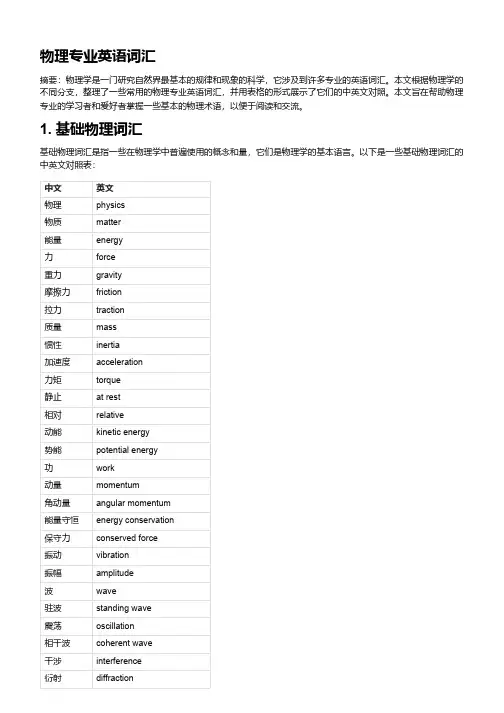
物理专业英语词汇摘要:物理学是一门研究自然界最基本的规律和现象的科学,它涉及到许多专业的英语词汇。
本文根据物理学的不同分支,整理了一些常用的物理专业英语词汇,并用表格的形式展示了它们的中英文对照。
本文旨在帮助物理专业的学习者和爱好者掌握一些基本的物理术语,以便于阅读和交流。
1. 基础物理词汇基础物理词汇是指一些在物理学中普遍使用的概念和量,它们是物理学的基本语言。
以下是一些基础物理词汇的中英文对照表:中文英文物理physics物质matter能量energy力force重力gravity摩擦力friction拉力traction质量mass惯性inertia加速度acceleration力矩torque静止at rest相对relative动能kinetic energy势能potential energy功work动量momentum角动量angular momentum能量守恒energy conservation保守力conserved force振动vibration振幅amplitude波wave驻波standing wave震荡oscillation相干波coherent wave干涉interference衍射diffraction轨道orbit速度velocity速率speed大小magnitude方向direction水平horizontal竖直vertical相互垂直perpendicular坐标coordinate直角坐标系Cartesian coordinate system极坐标系polar coordinate system2. 电学和磁学词汇电学和磁学是研究电荷、电流、电场、磁场等现象和规律的物理学分支,它们与光学、热学、原子物理等有着密切的联系。
以下是一些电学和磁学词汇的中英文对照表:中文英文电子electron电荷charge电流current电场electric field电通量electric flux电势electric potential导体conductor电介质dielectric绝缘体insulator电阻resistor电阻率resistivity电容capacitor3. 物理专业英语词汇物理专业英语词汇是指在物理学的学习和研究中经常使用的一些专业术语,它们涵盖了物理学的各个分支和领域,如力学、电磁学、光学、热学、量子力学等。
the historical development of quantum theory量子理论是二十世纪最重要的科学发现之一,它改变了我们对世界的认识。
量子理论的发展是一段漫长而充满曲折的历史。
以下是量子理论的历史发展:1900年,德国物理学家马克斯·普朗克提出了黑体辐射理论,这是量子理论的开端。
普朗克发现,无法用经典物理学解释黑体辐射的特性。
他假设能量是以离散的量子形式发射和吸收的,这个假设引发了量子化概念的诞生。
1905年,爱因斯坦在他的光电效应论文中提出了光是以粒子形式存在的理论,这个理论被称为光量子说,它也是量子理论的重要组成部分。
1913年,尼尔斯·玻尔提出了玻尔模型,该模型可以解释氢原子的光谱线。
这个模型的关键是电子只能在特定的能级中运动,并且电子在跃迁时会释放或吸收能量。
1925年,德国物理学家维尔纳·海森伯提出了著名的不确定性原理,它指出,我们不能同时精确地测量一个粒子的位置和动量。
这个原理改变了我们对粒子的认识。
1926年,奥地利物理学家埃尔温·薛定谔提出了薛定谔方程式,这个方程式描述了量子系统的演化。
它也是量子力学的基础。
1927年,英国物理学家保罗·狄拉克提出了狄拉克方程式,它描述了电子的行为,并预测了反物质的存在。
1935年,爱因斯坦、波多尔斯基和罗森提出了著名的EPR实验,这个实验证明了量子纠缠现象的存在。
这个实验也引发了量子信息学的发展。
以上是量子理论的历史发展的一些重要事件。
现在,量子理论已经成为现代物理学的重要分支,它在许多领域有着广泛的应用,包括计算机、通信和加密等。
爱因斯坦做出的贡献的英文作文阿尔伯特·爱因斯坦,这位二十世纪最伟大的理论物理学家之一,以其深邃的洞察力、无与伦比的创造力和对宇宙奥秘的不懈探索,为人类科学知识体系做出了诸多里程碑式的贡献。
他不仅彻底颠覆了人们对时空、物质和能量的传统认知,更奠定了现代物理学的两大基石——相对论和量子力学。
(English):Albert Einstein, one of the greatest theoretical physicists of the 20th century, made numerous landmark contributions to humanity's scientific knowledge system with his profound insights, unparalleled creativity, and relentless exploration of cosmic mysteries. He not only fundamentally upended traditional notions of space, time, matter, and energy but also laid the twin cornerstones of modern physics: relativity and quantum mechanics.Paragraph 2 (中文):爱因斯坦首先在1905年提出了狭义相对论,这是对牛顿力学框架的一次革命性突破。
他揭示了时间和空间并非绝对不变,而是相互关联、随观察者运动状态而变化的统一四维时空。
著名的质能方程E=mc²,便是这一理论的核心成果,它表明能量(E)与质量(m)之间存在着直接等价关系,且能量的转换蕴含着巨大的潜能。
这一发现不仅为核能的开发提供了理论基础,也深刻影响了我们对宇宙起源、星体演化等宏观现象的理解。
光子数密度Photons, the fundamental particles of light, play a crucial role in various physical processes and applications. One key concept related to photons is their number density, which refers to the number of photons per unit volume. This metric is particularly important in fields such as quantum optics, laser physics, and photodetection, where understanding the density of photons is crucial for accurate modeling and predictions.光子,作为光的基本粒子,在各种物理过程和应用中起着至关重要的作用。
与光子相关的一个关键概念是其数密度,即单位体积内的光子数量。
这一度量在量子光学、激光物理和光电探测等领域尤为重要,因为这些领域需要准确理解光子的密度才能进行精确的建模和预测。
In quantum optics, for instance, the photon number density determines the intensity of light and its interaction with matter.A higher photon number density corresponds to a brighter light source, which can lead to stronger interactions with atoms or molecules. This, in turn, affects the behavior of quantum systems and their ability to emit or absorb light.例如,在量子光学中,光子数密度决定了光的强度及其与物质的相互作用。

华中师范大学物理学院物理学专业英语仅供内部学习参考!2014一、课程的任务和教学目的通过学习《物理学专业英语》,学生将掌握物理学领域使用频率较高的专业词汇和表达方法,进而具备基本的阅读理解物理学专业文献的能力。
通过分析《物理学专业英语》课程教材中的范文,学生还将从英语角度理解物理学中个学科的研究内容和主要思想,提高学生的专业英语能力和了解物理学研究前沿的能力。
培养专业英语阅读能力,了解科技英语的特点,提高专业外语的阅读质量和阅读速度;掌握一定量的本专业英文词汇,基本达到能够独立完成一般性本专业外文资料的阅读;达到一定的笔译水平。
要求译文通顺、准确和专业化。
要求译文通顺、准确和专业化。
二、课程内容课程内容包括以下章节:物理学、经典力学、热力学、电磁学、光学、原子物理、统计力学、量子力学和狭义相对论三、基本要求1.充分利用课内时间保证充足的阅读量(约1200~1500词/学时),要求正确理解原文。
2.泛读适量课外相关英文读物,要求基本理解原文主要内容。
3.掌握基本专业词汇(不少于200词)。
4.应具有流利阅读、翻译及赏析专业英语文献,并能简单地进行写作的能力。
四、参考书目录1 Physics 物理学 (1)Introduction to physics (1)Classical and modern physics (2)Research fields (4)V ocabulary (7)2 Classical mechanics 经典力学 (10)Introduction (10)Description of classical mechanics (10)Momentum and collisions (14)Angular momentum (15)V ocabulary (16)3 Thermodynamics 热力学 (18)Introduction (18)Laws of thermodynamics (21)System models (22)Thermodynamic processes (27)Scope of thermodynamics (29)V ocabulary (30)4 Electromagnetism 电磁学 (33)Introduction (33)Electrostatics (33)Magnetostatics (35)Electromagnetic induction (40)V ocabulary (43)5 Optics 光学 (45)Introduction (45)Geometrical optics (45)Physical optics (47)Polarization (50)V ocabulary (51)6 Atomic physics 原子物理 (52)Introduction (52)Electronic configuration (52)Excitation and ionization (56)V ocabulary (59)7 Statistical mechanics 统计力学 (60)Overview (60)Fundamentals (60)Statistical ensembles (63)V ocabulary (65)8 Quantum mechanics 量子力学 (67)Introduction (67)Mathematical formulations (68)Quantization (71)Wave-particle duality (72)Quantum entanglement (75)V ocabulary (77)9 Special relativity 狭义相对论 (79)Introduction (79)Relativity of simultaneity (80)Lorentz transformations (80)Time dilation and length contraction (81)Mass-energy equivalence (82)Relativistic energy-momentum relation (86)V ocabulary (89)正文标记说明:蓝色Arial字体(例如energy):已知的专业词汇蓝色Arial字体加下划线(例如electromagnetism):新学的专业词汇黑色Times New Roman字体加下划线(例如postulate):新学的普通词汇1 Physics 物理学1 Physics 物理学Introduction to physicsPhysics is a part of natural philosophy and a natural science that involves the study of matter and its motion through space and time, along with related concepts such as energy and force. More broadly, it is the general analysis of nature, conducted in order to understand how the universe behaves.Physics is one of the oldest academic disciplines, perhaps the oldest through its inclusion of astronomy. Over the last two millennia, physics was a part of natural philosophy along with chemistry, certain branches of mathematics, and biology, but during the Scientific Revolution in the 17th century, the natural sciences emerged as unique research programs in their own right. Physics intersects with many interdisciplinary areas of research, such as biophysics and quantum chemistry,and the boundaries of physics are not rigidly defined. New ideas in physics often explain the fundamental mechanisms of other sciences, while opening new avenues of research in areas such as mathematics and philosophy.Physics also makes significant contributions through advances in new technologies that arise from theoretical breakthroughs. For example, advances in the understanding of electromagnetism or nuclear physics led directly to the development of new products which have dramatically transformed modern-day society, such as television, computers, domestic appliances, and nuclear weapons; advances in thermodynamics led to the development of industrialization; and advances in mechanics inspired the development of calculus.Core theoriesThough physics deals with a wide variety of systems, certain theories are used by all physicists. Each of these theories were experimentally tested numerous times and found correct as an approximation of nature (within a certain domain of validity).For instance, the theory of classical mechanics accurately describes the motion of objects, provided they are much larger than atoms and moving at much less than the speed of light. These theories continue to be areas of active research, and a remarkable aspect of classical mechanics known as chaos was discovered in the 20th century, three centuries after the original formulation of classical mechanics by Isaac Newton (1642–1727) 【艾萨克·牛顿】.University PhysicsThese central theories are important tools for research into more specialized topics, and any physicist, regardless of his or her specialization, is expected to be literate in them. These include classical mechanics, quantum mechanics, thermodynamics and statistical mechanics, electromagnetism, and special relativity.Classical and modern physicsClassical mechanicsClassical physics includes the traditional branches and topics that were recognized and well-developed before the beginning of the 20th century—classical mechanics, acoustics, optics, thermodynamics, and electromagnetism.Classical mechanics is concerned with bodies acted on by forces and bodies in motion and may be divided into statics (study of the forces on a body or bodies at rest), kinematics (study of motion without regard to its causes), and dynamics (study of motion and the forces that affect it); mechanics may also be divided into solid mechanics and fluid mechanics (known together as continuum mechanics), the latter including such branches as hydrostatics, hydrodynamics, aerodynamics, and pneumatics.Acoustics is the study of how sound is produced, controlled, transmitted and received. Important modern branches of acoustics include ultrasonics, the study of sound waves of very high frequency beyond the range of human hearing; bioacoustics the physics of animal calls and hearing, and electroacoustics, the manipulation of audible sound waves using electronics.Optics, the study of light, is concerned not only with visible light but also with infrared and ultraviolet radiation, which exhibit all of the phenomena of visible light except visibility, e.g., reflection, refraction, interference, diffraction, dispersion, and polarization of light.Heat is a form of energy, the internal energy possessed by the particles of which a substance is composed; thermodynamics deals with the relationships between heat and other forms of energy.Electricity and magnetism have been studied as a single branch of physics since the intimate connection between them was discovered in the early 19th century; an electric current gives rise to a magnetic field and a changing magnetic field induces an electric current. Electrostatics deals with electric charges at rest, electrodynamics with moving charges, and magnetostatics with magnetic poles at rest.Modern PhysicsClassical physics is generally concerned with matter and energy on the normal scale of1 Physics 物理学observation, while much of modern physics is concerned with the behavior of matter and energy under extreme conditions or on the very large or very small scale.For example, atomic and nuclear physics studies matter on the smallest scale at which chemical elements can be identified.The physics of elementary particles is on an even smaller scale, as it is concerned with the most basic units of matter; this branch of physics is also known as high-energy physics because of the extremely high energies necessary to produce many types of particles in large particle accelerators. On this scale, ordinary, commonsense notions of space, time, matter, and energy are no longer valid.The two chief theories of modern physics present a different picture of the concepts of space, time, and matter from that presented by classical physics.Quantum theory is concerned with the discrete, rather than continuous, nature of many phenomena at the atomic and subatomic level, and with the complementary aspects of particles and waves in the description of such phenomena.The theory of relativity is concerned with the description of phenomena that take place in a frame of reference that is in motion with respect to an observer; the special theory of relativity is concerned with relative uniform motion in a straight line and the general theory of relativity with accelerated motion and its connection with gravitation.Both quantum theory and the theory of relativity find applications in all areas of modern physics.Difference between classical and modern physicsWhile physics aims to discover universal laws, its theories lie in explicit domains of applicability. Loosely speaking, the laws of classical physics accurately describe systems whose important length scales are greater than the atomic scale and whose motions are much slower than the speed of light. Outside of this domain, observations do not match their predictions.Albert Einstein【阿尔伯特·爱因斯坦】contributed the framework of special relativity, which replaced notions of absolute time and space with space-time and allowed an accurate description of systems whose components have speeds approaching the speed of light.Max Planck【普朗克】, Erwin Schrödinger【薛定谔】, and others introduced quantum mechanics, a probabilistic notion of particles and interactions that allowed an accurate description of atomic and subatomic scales.Later, quantum field theory unified quantum mechanics and special relativity.General relativity allowed for a dynamical, curved space-time, with which highly massiveUniversity Physicssystems and the large-scale structure of the universe can be well-described. General relativity has not yet been unified with the other fundamental descriptions; several candidate theories of quantum gravity are being developed.Research fieldsContemporary research in physics can be broadly divided into condensed matter physics; atomic, molecular, and optical physics; particle physics; astrophysics; geophysics and biophysics. Some physics departments also support research in Physics education.Since the 20th century, the individual fields of physics have become increasingly specialized, and today most physicists work in a single field for their entire careers. "Universalists" such as Albert Einstein (1879–1955) and Lev Landau (1908–1968)【列夫·朗道】, who worked in multiple fields of physics, are now very rare.Condensed matter physicsCondensed matter physics is the field of physics that deals with the macroscopic physical properties of matter. In particular, it is concerned with the "condensed" phases that appear whenever the number of particles in a system is extremely large and the interactions between them are strong.The most familiar examples of condensed phases are solids and liquids, which arise from the bonding by way of the electromagnetic force between atoms. More exotic condensed phases include the super-fluid and the Bose–Einstein condensate found in certain atomic systems at very low temperature, the superconducting phase exhibited by conduction electrons in certain materials,and the ferromagnetic and antiferromagnetic phases of spins on atomic lattices.Condensed matter physics is by far the largest field of contemporary physics.Historically, condensed matter physics grew out of solid-state physics, which is now considered one of its main subfields. The term condensed matter physics was apparently coined by Philip Anderson when he renamed his research group—previously solid-state theory—in 1967. In 1978, the Division of Solid State Physics of the American Physical Society was renamed as the Division of Condensed Matter Physics.Condensed matter physics has a large overlap with chemistry, materials science, nanotechnology and engineering.Atomic, molecular and optical physicsAtomic, molecular, and optical physics (AMO) is the study of matter–matter and light–matter interactions on the scale of single atoms and molecules.1 Physics 物理学The three areas are grouped together because of their interrelationships, the similarity of methods used, and the commonality of the energy scales that are relevant. All three areas include both classical, semi-classical and quantum treatments; they can treat their subject from a microscopic view (in contrast to a macroscopic view).Atomic physics studies the electron shells of atoms. Current research focuses on activities in quantum control, cooling and trapping of atoms and ions, low-temperature collision dynamics and the effects of electron correlation on structure and dynamics. Atomic physics is influenced by the nucleus (see, e.g., hyperfine splitting), but intra-nuclear phenomena such as fission and fusion are considered part of high-energy physics.Molecular physics focuses on multi-atomic structures and their internal and external interactions with matter and light.Optical physics is distinct from optics in that it tends to focus not on the control of classical light fields by macroscopic objects, but on the fundamental properties of optical fields and their interactions with matter in the microscopic realm.High-energy physics (particle physics) and nuclear physicsParticle physics is the study of the elementary constituents of matter and energy, and the interactions between them.In addition, particle physicists design and develop the high energy accelerators,detectors, and computer programs necessary for this research. The field is also called "high-energy physics" because many elementary particles do not occur naturally, but are created only during high-energy collisions of other particles.Currently, the interactions of elementary particles and fields are described by the Standard Model.●The model accounts for the 12 known particles of matter (quarks and leptons) thatinteract via the strong, weak, and electromagnetic fundamental forces.●Dynamics are described in terms of matter particles exchanging gauge bosons (gluons,W and Z bosons, and photons, respectively).●The Standard Model also predicts a particle known as the Higgs boson. In July 2012CERN, the European laboratory for particle physics, announced the detection of a particle consistent with the Higgs boson.Nuclear Physics is the field of physics that studies the constituents and interactions of atomic nuclei. The most commonly known applications of nuclear physics are nuclear power generation and nuclear weapons technology, but the research has provided application in many fields, including those in nuclear medicine and magnetic resonance imaging, ion implantation in materials engineering, and radiocarbon dating in geology and archaeology.University PhysicsAstrophysics and Physical CosmologyAstrophysics and astronomy are the application of the theories and methods of physics to the study of stellar structure, stellar evolution, the origin of the solar system, and related problems of cosmology. Because astrophysics is a broad subject, astrophysicists typically apply many disciplines of physics, including mechanics, electromagnetism, statistical mechanics, thermodynamics, quantum mechanics, relativity, nuclear and particle physics, and atomic and molecular physics.The discovery by Karl Jansky in 1931 that radio signals were emitted by celestial bodies initiated the science of radio astronomy. Most recently, the frontiers of astronomy have been expanded by space exploration. Perturbations and interference from the earth's atmosphere make space-based observations necessary for infrared, ultraviolet, gamma-ray, and X-ray astronomy.Physical cosmology is the study of the formation and evolution of the universe on its largest scales. Albert Einstein's theory of relativity plays a central role in all modern cosmological theories. In the early 20th century, Hubble's discovery that the universe was expanding, as shown by the Hubble diagram, prompted rival explanations known as the steady state universe and the Big Bang.The Big Bang was confirmed by the success of Big Bang nucleo-synthesis and the discovery of the cosmic microwave background in 1964. The Big Bang model rests on two theoretical pillars: Albert Einstein's general relativity and the cosmological principle (On a sufficiently large scale, the properties of the Universe are the same for all observers). Cosmologists have recently established the ΛCDM model (the standard model of Big Bang cosmology) of the evolution of the universe, which includes cosmic inflation, dark energy and dark matter.Current research frontiersIn condensed matter physics, an important unsolved theoretical problem is that of high-temperature superconductivity. Many condensed matter experiments are aiming to fabricate workable spintronics and quantum computers.In particle physics, the first pieces of experimental evidence for physics beyond the Standard Model have begun to appear. Foremost among these are indications that neutrinos have non-zero mass. These experimental results appear to have solved the long-standing solar neutrino problem, and the physics of massive neutrinos remains an area of active theoretical and experimental research. Particle accelerators have begun probing energy scales in the TeV range, in which experimentalists are hoping to find evidence for the super-symmetric particles, after discovery of the Higgs boson.Theoretical attempts to unify quantum mechanics and general relativity into a single theory1 Physics 物理学of quantum gravity, a program ongoing for over half a century, have not yet been decisively resolved. The current leading candidates are M-theory, superstring theory and loop quantum gravity.Many astronomical and cosmological phenomena have yet to be satisfactorily explained, including the existence of ultra-high energy cosmic rays, the baryon asymmetry, the acceleration of the universe and the anomalous rotation rates of galaxies.Although much progress has been made in high-energy, quantum, and astronomical physics, many everyday phenomena involving complexity, chaos, or turbulence are still poorly understood. Complex problems that seem like they could be solved by a clever application of dynamics and mechanics remain unsolved; examples include the formation of sand-piles, nodes in trickling water, the shape of water droplets, mechanisms of surface tension catastrophes, and self-sorting in shaken heterogeneous collections.These complex phenomena have received growing attention since the 1970s for several reasons, including the availability of modern mathematical methods and computers, which enabled complex systems to be modeled in new ways. Complex physics has become part of increasingly interdisciplinary research, as exemplified by the study of turbulence in aerodynamics and the observation of pattern formation in biological systems.Vocabulary★natural science 自然科学academic disciplines 学科astronomy 天文学in their own right 凭他们本身的实力intersects相交,交叉interdisciplinary交叉学科的,跨学科的★quantum 量子的theoretical breakthroughs 理论突破★electromagnetism 电磁学dramatically显著地★thermodynamics热力学★calculus微积分validity★classical mechanics 经典力学chaos 混沌literate 学者★quantum mechanics量子力学★thermodynamics and statistical mechanics热力学与统计物理★special relativity狭义相对论is concerned with 关注,讨论,考虑acoustics 声学★optics 光学statics静力学at rest 静息kinematics运动学★dynamics动力学ultrasonics超声学manipulation 操作,处理,使用University Physicsinfrared红外ultraviolet紫外radiation辐射reflection 反射refraction 折射★interference 干涉★diffraction 衍射dispersion散射★polarization 极化,偏振internal energy 内能Electricity电性Magnetism 磁性intimate 亲密的induces 诱导,感应scale尺度★elementary particles基本粒子★high-energy physics 高能物理particle accelerators 粒子加速器valid 有效的,正当的★discrete离散的continuous 连续的complementary 互补的★frame of reference 参照系★the special theory of relativity 狭义相对论★general theory of relativity 广义相对论gravitation 重力,万有引力explicit 详细的,清楚的★quantum field theory 量子场论★condensed matter physics凝聚态物理astrophysics天体物理geophysics地球物理Universalist博学多才者★Macroscopic宏观Exotic奇异的★Superconducting 超导Ferromagnetic铁磁质Antiferromagnetic 反铁磁质★Spin自旋Lattice 晶格,点阵,网格★Society社会,学会★microscopic微观的hyperfine splitting超精细分裂fission分裂,裂变fusion熔合,聚变constituents成分,组分accelerators加速器detectors 检测器★quarks夸克lepton 轻子gauge bosons规范玻色子gluons胶子★Higgs boson希格斯玻色子CERN欧洲核子研究中心★Magnetic Resonance Imaging磁共振成像,核磁共振ion implantation 离子注入radiocarbon dating放射性碳年代测定法geology地质学archaeology考古学stellar 恒星cosmology宇宙论celestial bodies 天体Hubble diagram 哈勃图Rival竞争的★Big Bang大爆炸nucleo-synthesis核聚合,核合成pillar支柱cosmological principle宇宙学原理ΛCDM modelΛ-冷暗物质模型cosmic inflation宇宙膨胀1 Physics 物理学fabricate制造,建造spintronics自旋电子元件,自旋电子学★neutrinos 中微子superstring 超弦baryon重子turbulence湍流,扰动,骚动catastrophes突变,灾变,灾难heterogeneous collections异质性集合pattern formation模式形成University Physics2 Classical mechanics 经典力学IntroductionIn physics, classical mechanics is one of the two major sub-fields of mechanics, which is concerned with the set of physical laws describing the motion of bodies under the action of a system of forces. The study of the motion of bodies is an ancient one, making classical mechanics one of the oldest and largest subjects in science, engineering and technology.Classical mechanics describes the motion of macroscopic objects, from projectiles to parts of machinery, as well as astronomical objects, such as spacecraft, planets, stars, and galaxies. Besides this, many specializations within the subject deal with gases, liquids, solids, and other specific sub-topics.Classical mechanics provides extremely accurate results as long as the domain of study is restricted to large objects and the speeds involved do not approach the speed of light. When the objects being dealt with become sufficiently small, it becomes necessary to introduce the other major sub-field of mechanics, quantum mechanics, which reconciles the macroscopic laws of physics with the atomic nature of matter and handles the wave–particle duality of atoms and molecules. In the case of high velocity objects approaching the speed of light, classical mechanics is enhanced by special relativity. General relativity unifies special relativity with Newton's law of universal gravitation, allowing physicists to handle gravitation at a deeper level.The initial stage in the development of classical mechanics is often referred to as Newtonian mechanics, and is associated with the physical concepts employed by and the mathematical methods invented by Newton himself, in parallel with Leibniz【莱布尼兹】, and others.Later, more abstract and general methods were developed, leading to reformulations of classical mechanics known as Lagrangian mechanics and Hamiltonian mechanics. These advances were largely made in the 18th and 19th centuries, and they extend substantially beyond Newton's work, particularly through their use of analytical mechanics. Ultimately, the mathematics developed for these were central to the creation of quantum mechanics.Description of classical mechanicsThe following introduces the basic concepts of classical mechanics. For simplicity, it often2 Classical mechanics 经典力学models real-world objects as point particles, objects with negligible size. The motion of a point particle is characterized by a small number of parameters: its position, mass, and the forces applied to it.In reality, the kind of objects that classical mechanics can describe always have a non-zero size. (The physics of very small particles, such as the electron, is more accurately described by quantum mechanics). Objects with non-zero size have more complicated behavior than hypothetical point particles, because of the additional degrees of freedom—for example, a baseball can spin while it is moving. However, the results for point particles can be used to study such objects by treating them as composite objects, made up of a large number of interacting point particles. The center of mass of a composite object behaves like a point particle.Classical mechanics uses common-sense notions of how matter and forces exist and interact. It assumes that matter and energy have definite, knowable attributes such as where an object is in space and its speed. It also assumes that objects may be directly influenced only by their immediate surroundings, known as the principle of locality.In quantum mechanics objects may have unknowable position or velocity, or instantaneously interact with other objects at a distance.Position and its derivativesThe position of a point particle is defined with respect to an arbitrary fixed reference point, O, in space, usually accompanied by a coordinate system, with the reference point located at the origin of the coordinate system. It is defined as the vector r from O to the particle.In general, the point particle need not be stationary relative to O, so r is a function of t, the time elapsed since an arbitrary initial time.In pre-Einstein relativity (known as Galilean relativity), time is considered an absolute, i.e., the time interval between any given pair of events is the same for all observers. In addition to relying on absolute time, classical mechanics assumes Euclidean geometry for the structure of space.Velocity and speedThe velocity, or the rate of change of position with time, is defined as the derivative of the position with respect to time. In classical mechanics, velocities are directly additive and subtractive as vector quantities; they must be dealt with using vector analysis.When both objects are moving in the same direction, the difference can be given in terms of speed only by ignoring direction.University PhysicsAccelerationThe acceleration , or rate of change of velocity, is the derivative of the velocity with respect to time (the second derivative of the position with respect to time).Acceleration can arise from a change with time of the magnitude of the velocity or of the direction of the velocity or both . If only the magnitude v of the velocity decreases, this is sometimes referred to as deceleration , but generally any change in the velocity with time, including deceleration, is simply referred to as acceleration.Inertial frames of referenceWhile the position and velocity and acceleration of a particle can be referred to any observer in any state of motion, classical mechanics assumes the existence of a special family of reference frames in terms of which the mechanical laws of nature take a comparatively simple form. These special reference frames are called inertial frames .An inertial frame is such that when an object without any force interactions (an idealized situation) is viewed from it, it appears either to be at rest or in a state of uniform motion in a straight line. This is the fundamental definition of an inertial frame. They are characterized by the requirement that all forces entering the observer's physical laws originate in identifiable sources (charges, gravitational bodies, and so forth).A non-inertial reference frame is one accelerating with respect to an inertial one, and in such a non-inertial frame a particle is subject to acceleration by fictitious forces that enter the equations of motion solely as a result of its accelerated motion, and do not originate in identifiable sources. These fictitious forces are in addition to the real forces recognized in an inertial frame.A key concept of inertial frames is the method for identifying them. For practical purposes, reference frames that are un-accelerated with respect to the distant stars are regarded as good approximations to inertial frames.Forces; Newton's second lawNewton was the first to mathematically express the relationship between force and momentum . Some physicists interpret Newton's second law of motion as a definition of force and mass, while others consider it a fundamental postulate, a law of nature. Either interpretation has the same mathematical consequences, historically known as "Newton's Second Law":a m t v m t p F ===d )(d d dThe quantity m v is called the (canonical ) momentum . The net force on a particle is thus equal to rate of change of momentum of the particle with time.So long as the force acting on a particle is known, Newton's second law is sufficient to。
高Q 值二维光子晶体微腔光子腔具有约束光线的特性,这个特性可以应用到物理和工程的许多领域中,包括相关电-光互相作用[1],超小滤光片[2,3],低阈值激光器[4],光子芯片[5],非线性光学[6]和处理量子信息[7]。
这些应用的关键是实现腔的品质因数Q,更小的模式体积。
比例Q/V决定了各种腔的互相作用强度,和一个超小型腔使能够大范围互相作用和更宽波长范围的单模运算。
可是一个高Q光波长的腔范围是很难制作,因为辐射损失与腔的体积成反比。
除了一些最近的理论研究,在制造高Q值微腔方面没有权威的理论和实验[8-10]。
在这里我们使用基于硅的二维光子晶体平板微腔,Q=45,000和V=7.0x10⁻¹⁴cm3;Q/V值是以前研究的10-100倍。
这项研究使我们意识到光线可以被更强烈的约束[4,11-14]。
集成与其他光子器件是非常简单的,已经可以证明100nm的光谱范围了。
腔的Q值决定于相对于原能量的每个周期的能量损耗。
由于腔的材料对光没有吸收,Q值决定于腔内外界面之间的能量损失。
全部内部反射(TIR)和/或布拉格散射常用于对光的约束。
对于一个体积大于光波长的腔,已经可以得到一个很高的Q值了[14,15。
在这种情况下,被约束在腔中的光线符合光学理论,每一束在交界面处被反射的光都符合全内反射或布拉格散射。
腔越小光线对光学理论的偏移越严重,因此Q值会变小。
被约束在微腔中的光线是由非常多的平面波组成的,由于光的局部化这些平面波是由很多波矢k组成。
设计出符合全内反射或者布拉格散射的平面波非常困难,高Q值光子晶体谐振腔的产生很好的解决这个问题。
解决这个问题的一个很好的办法就是在所有方向上运用布拉格散射效应。
二维或者三维的折射率周期性变化的结构可以产生这样的效应,变化基于光波波长的数量级。
这些被称为光子晶体,类似于固体晶体[5,16]。
对于一个三维光子晶体,布拉格散射可以约束所有方向特定频率范围的光线,称为光子带隙。
一个小扰动或缺陷引入三维光子晶体就会形成光子晶体微谐振腔,并具有极高的Q/V值。
Bose-Einstein condensationShihao LiBJTU ID#:13276013;UW ID#:20548261School of Science,Beijing Jiaotong University,Beijing,100044,ChinaJune1,20151What is BEC?To answer this question,it has to begin with the fermions and bosons.As is known,matters consist of atoms,atoms are made of protons,neutrons and electrons, and protons and neutrons are made of quarks.Also,there are photons and gluons that works for transferring interaction.All of these particles are microscopic particles and can be classified to two families,the fermion and the boson.A fermion is any particle characterized by Fermi–Dirac statistics.Particles with half-integer spin are fermions,including all quarks,leptons and electrons,as well as any composite particle made of an odd number of these,such as all baryons and many atoms and nuclei.As a consequence of the Pauli exclusion principle,two or more identical fermions cannot occupy the same quantum state at any given time.Differing from fermions,bosons obey Bose-Einstein statistics.Particles with integer spin are bosons,such as photons,gluons,W and Z bosons,the Higgs boson, and the still-theoretical graviton of quantum gravity.It also includes the composite particle made of even number of fermions,such as the nuclei with even number ofnucleons.An important characteristic of bosons is that their statistics do not restrict the number of them that occupy the same quantum state.For a single particle,when the temperature is at the absolute zero,0K,the particle is in the state of lowest energy,the ground state.Supposing that there are many particle,if they are fermions,there will be exactly one of them in the ground state;if they are bosons,most of them will be in the ground state,where these bosons share the same quantum states,and this state is called Bose-Einstein condensate (BEC).Bose–Einstein condensation(BEC)—the macroscopic groundstate accumulation of particles of a dilute gas with integer spin(bosons)at high density and low temperature very close to absolute zero.According to the knowledge of quantum mechanics,all microscopic particles have the wave-particle duality.For an atom in space,it can be expressed as well as a wave function.As is shown in the figure1.1,it tells the distribution but never exact position of atoms.Each distribution corresponds to the de Broglie wavelength of each atom.Lower the temperature is,lower the kinetic energy is,and longer the de Broglie wavelength is.p=mv=h/λ(Eq.1.1)When the distance of atoms is less than the de Broglie wavelength,the distribution of atoms are overlapped,like figure1.2.For the atoms of the same category,the overlapped distribution leads to a integral quantum state.If those atoms are bosons,each member will tend to a particular quantum state,and the whole atomsystem will become the BEC.In BEC,the physical property of all atoms is totally identical,and they are indistinguishable and like one independent atom.Figure1.1Wave functionsFigure1.2Overlapped wave functionWhat should be stressed is that the Bose–Einstein condensate is based on bosons, and BEC is a macroscopic quantum state.The first time people obtained BEC of gaseous rubidium atoms at170nK in lab was1995.Up to now,physicists have found the BEC of eight elements,most of which are alkali metals,calcium,and helium-4 atom.Always,the BEC of atom has some amazing properties which plays a vital role in the application of chip technology,precision measurement,and nano technology. What’s more,as a macroscopic quantum state,Bose–Einstein condensate gives a brand new research approach and field.2Bose and Einstein's papers were published in1924.Why does it take so long before it can be observed experimentally in atoms in1995?The condition of obtaining the BEC is daunting in1924.On the one hand,the temperature has to approach the absolute zero indefinitely;on the other hand,the aimed sample atoms should have relatively high density with few interactions but still keep in gaseous state.However,most categories of atom will easily tend to combine with others and form gaseous molecules or liquid.At first,people focused on the BEC of hydrogen atom,but failed to in the end. Fortunately,after the research,the alkali metal atoms with one electron in the outer shell and odd number of nuclei spin,which can be seen as bosons,were found suitable to obtain BEC in1980s.This is the first reason why it takes so long before BEC can be observed.Then,here’s a problem of cooling atom.Cooling atom make the kinetic energy of atom less.The breakthrough appeared in1960s when the laser was invented.In1975, the idea of laser cooling was advanced by Hänsch and Shallow.Here’s a chart of the development of laser cooling:Year Technique Limit Temperature Contributors 1980~Laser cooling of the atomic beam~mK Phillips,etc. 19853-D Laser cooling~240μK S.Chu,etc. 1989Sisyphus cooling~0.1~1μK Dalibard,etc. 1995Evaporative cooling~100nK S.Chu,etc. 1995The first realization of BEC~20nK JILA group Until1995,people didn’t have the cooling technique which was not perfect enough,so that’s the other answer.By the way,the Nobel Prize in Physics1997wasawarded to Stephen Chu,Claude Cohen-Tannoudji,and William D.Phillips for the contribution on laser cooling and trapping of atoms.3Anything you can add to the BEC phenomena(recent developments,etc.)from your own Reading.Bose–Einstein condensation of photons in an optical microcavity BEC is the state of bosons at extremely low temperature.According to the traditional view,photon does not have static mass,which means lower the temperature is,less the number of photons will be.It's very difficult for scientists to get Bose Einstein condensation of photons.Several German scientists said they obtained the BEC of photon successfully in the journal Nature published on November24th,2011.Their experiment confines photons in a curved-mirror optical microresonator filled with a dye solution,in which photons are repeatedly absorbed and re-emitted by the dye molecules.Those photons could‘heat’the dye molecules and be gradually cooled.The small distance of3.5 optical wavelengths between the mirrors causes a large frequency spacing between adjacent longitudinal modes.By pumping the dye with an external laser we add to a reservoir of electronic excitations that exchanges particles with the photon gas,in the sense of a grand-canonical ensemble.The pumping is maintained throughout the measurement to compensate for losses due to coupling into unconfined optical modes, finite quantum efficiency and mirror losses until they reach a steady state and become a super photons.(Klaers,J.,Schmitt,J.,Vewinger, F.,&Weitz,M.(2010).Bose-einstein condensation of photons in an optical microcavity.Nature,468(7323), 545-548.)With the BEC of photons,a brand new light source is created,which gives a possible to generate laser with extremely short wavelength,such as UV laser and X-ray laser.What’s more,it shows the future of powerful computer chip.Figure3.1Scheme of the experimental setup.4ConclusionA Bose-Einstein condensation(BEC)is a state of matter of a dilute gas of bosons cooled to temperatures very close to absolute zero.Under such conditions,a large fraction of bosons occupy the lowest quantum state,at which point macroscopic quantum phenomena become apparent.This state was first predicted,generally,in1924-25by Satyendra Nath Bose and Albert Einstein.And after70years,the Nobel Prize in Physics2001was awarded jointly to Eric A.Cornell,Wolfgang Ketterle and Carl E.Wieman"for theachievement of Bose-Einstein condensation in dilute gases of alkali atoms,and for early fundamental studies of the properties of the condensates".This achievement is not only related to the BEC theory but also the revolution of atom-cooling technique.5References[1]Pethick,C.,&Smith,H.(2001).Bose-einstein condensation in dilute gases.Bose-Einstein Condensation in Dilute Gases,56(6),414.[2]Klaers J,Schmitt J,Vewinger F,et al.Bose-Einstein condensation of photons in anoptical microcavity[J].Nature,2010,468(7323):545-548.[3]陈徐宗,&陈帅.(2002).物质的新状态——玻色-爱因斯坦凝聚——2001年诺贝尔物理奖介绍.物理,31(3),141-145.[4]Boson(n.d.)In Wikipedia.Retrieved from:</wiki/Boson>[5]Fermion(n.d.)In Wikipedia.Retrieved from:</wiki/Fermion>[6]Bose-einstein condensate(n.d.)In Wikipedia.Retrieved from:</wiki/Bose%E2%80%93Einstein_condensate>[7]玻色-爱因斯坦凝聚态(n.d.)In Baidubaike.Retrieved from:</link?url=5NzWN5riyBWC-qgPhvZ1QBcD2rdd4Tenkcw EyoEcOBhjh7-ofFra6uydj2ChtL-JvkPK78twjkfIC2gG2m_ZdK>。
霍金的简介英文版斯蒂芬威廉霍金,英国剑桥大学著名物理学家,20世纪享有国际盛誉的伟人之一,斯蒂芬威廉霍金简介Stephen William Hawking, born in Oxford, England on January 8, 1942, won CH (British Lord of Honor), CBE (British Empire mander Medal), FRS (Royal Society Member), FRSA (British Royal Art Association members) and other honors. He is a famous physicist at Cambridge University, one of the greatest physicists of modern times and one of the great men of the 20th century.He suffers from muscular atrophic lateral sclerosis (Luganle’s disease), generalized paralysis, can not speak, hand only three fingers can be active.From 1979 to 20xx, he was a professor of mathematics at Lucas. He was the most respected professor in Britain. Hawking’s main research field is cosmology and black hole, which proves the singularity theorem and black hole area theorem of general relativity, and puts forward the black hole evaporation theory and the boundless Hawking cosmic model. In the process of unifying the two basic theories of physics in the 20th century, Einstein founded the theory of relativity and Planck’s quantum mechanics to create an important step forward.斯蒂芬威廉霍金主要成就Stephen William Hawking’s research laid the groundwork for today’s understanding of the black hole and the origin of the universe, but according to himself, he said that he was in the animated The Simpsons and the science fiction episode Star Trek: Next Generation (Star Trek: The Next Generation) is also wonderful.Hawking emphasizes that the universe does not need a Creator or God in the Great Design, philosophy is dead, which means that mankind will be detached from ignorant self-slavery, denying that pure philosophy andreligion can really explain Naturally, it also shows that the major religions are only the ancient spiritual world to explore the unknown, the pursuit of immortal system, rather than the objective truth. With the progress of the times, human civilization is also catch up, not far behind, which is why generations of people of insight to the existence of life and the meaning of the universe. To solve these propositions should have been the task of the philosopher, but unfortunately the highly developed science makes the philosophy can not keep up. Hawking in the big design of the opening that philosophy is dead is the meaning.Hawking hopes to solve the mystery of the birth of the universe, the 1970s, Hawking quantum mechanics applied to explain the phenomenon of black hole, in the next 30 years, with quantum mechanics to explain the universe has bee more difficult. Hawking wanted to find a set of theories that could explain the universe as a whole to illustrate the birth of the billion years of the universe until now, but it has not been concluded for years even if it is infinitely close. According to his theory of quantum mechanics, the birth of the universe is the big bang produced, which is a pressed infinitely small but with large gravity of the material (also can be understood as the density of infinite) explosion products. The theoretical category of quantum mechanics can not explain how this process is going to be done. Why is it so? Hawking says that must have a theory that can describe small-scale gravity.The latest scientific breakthrough is Hawking’s colleague, Michael Smith of London’s Queen Mary’s College (Michael. Green) involved in the construction of the superstring theory, referred to as string theory, which states that all particles and natural forces are actually in shock In the universe like a small object, to solve the Hawking has always wanted to try to answer the gravity problem, this theory must be established in the universe must have 9,10 or even greater than 11 dimensions, and humanbeings in the three-dimensional world may only One of the real ones of the universe ...A large number of scientists around the world are doing experiments in space and earth to prove string theory and from experiments to support Hawking’s black hole theory and quantum theory. January 24, 20xx, the famous British scientist Professor Stephen Hawking once again with its black hole-related theory shocked the physics, in a recently published paper admitted that black hole does not exist, but gray hole indeed exist. In a paper entitled Information Preservation and Weather Forecasting For Black Holes, Hawking points out that black holes do not exist because they can not find the boundaries of black holes. In order to solve the firewall problem in the new theory set black hole does not exist, it does not really do not exist. The black hole of the boundary, also known as the horizon, the classic black hole theory that the black hole outside the material and radiation can enter the black hole through the horizon, and any material and radiation within the black hole can not wear out horizons.Hawking’s latest gray hole theory that material and energy in the black hole trapped after a period of time, will be re-released into the universe. He admitted in his essay that his initial knowledge of the horizon was flawed, and that light could cross the horizon. When the light flies the black hole core, its movement is like a person running on a treadmill, slowly through the outward radiation and shrink. The classical black hole theory argues that any matter and radiation can not escape the black hole, and quantum mechanics suggests that energy and information can escape from the black hole. Hawking also pointed out that the interpretation of this escape process requires a gravity And other basic forces of successful integration of the theory. In the past hundred years, no one in physics has tried to explain this process.For Hawking’s gray hole theory, some scientists expressed approval,it was skeptical. Joseph Polchinski, a theoretical physicist at the Cuban Institute of Theoretical Physics, points out that according to Einstein’s theory of gravity, the boundary of the black hole is present, but it differs from the rest of the universe Not obvious. In fact, as early as 20xx, Hawking had made a similar statement. On July 21 of that year, Hawking pointed out at the 17th International Symposium on General Theory of Relativity and Gravitation that the Black Hole was not pletely swallowed around it, as he and most other physicists had previously thought, Some of the information that is sucked into the depths of the black hole may be released at some point.In 1973, Hawking said he calculated by the conclusion that the black hole in the formation of the process of its quality reduction, but also continue to be in the form of energy to the outside world radiation. This is the famous Hawking radiation theory, the theory mentioned in the black hole radiation does not include the black hole inside the material of any information, once the black hole is concentrated and evaporated disappear, all of which information will disappear, which is the so-called The black hole paradox. This theory and quantum mechanics of the relevant theories appear contradictory. Because modern quantum physics finds that this material information is never pletely gone.For more than 30 years, Hawking tried to explain this contradictory view with various speculations. Hawking has said that the quantum movement of the black hole is a special case, because the gravity in the black hole is very strong, quantum mechanics at this time is no longer applicable. Hawking’s argument does not convince the scienti fic munity of skeptical scholars. It now appears that Hawking finally gave this year’s contradictory view of a more convincing answer. Hawking said the black hole never pletely shut itself - Hawking radiation, they in a long period of time gradually to the outside world to radiate more and more heat, thenthe black hole will eventually open themselves and release the material contained in the information.On August 16, 1616, Jeff Steinhauer, a professor at the Israel Institute of Technology in Haifa, proved the quantum effect of Hawking radiation in a paper published in the journal Nature Physics. He made a sound black hole instead of a light black hole, using a long tube with sound particles, the phonon horizon. In 20xx, Professor Steinhall found that the phonemes were randomly generated in the horizon. In his latest results, Steinhouse proved that these phonons were one of a pair of related phonons, thus proving the quantum effect of Hawking radiation.斯蒂芬威廉霍金社会活动April 12, 20xx, the famous British physicist Stephen Hawking in New York New World Trade Center Observatory announced a plan called breakthrough star plan, with the Russian businessman Yuri Milner, the US social networking site Facebook Founder Zuckerberg collaborated to build a new space exploration project, build a large number of miniature interplanetary spaceships and launch them at half the speed of light to the Centaur Alpha Star. The day was the sixth international manned space day established by the United Nations and the 55th anniversary of the first manned space flight.Milner said at a press conference that the initial investment in the Breakthrough Star program would be $ 100 million to develop a miniature interplanetary spacecraft using laser propulsion and to fly to Centauri in the current generation of time Star of the target.According to reports, plans to build a miniature interstellar spacecraft called nano-aircraft, which consists of a star puter chip as a hull. Milner at the press conference to show the star of the original product. The chip is only two or three centimeters square, a few grams of weight, but integrated camera, photon thruster, navigation andtransmission ponents, is a plete space exploration function of the aircraft, and manufacturing costs only equivalent to an iPhone.The chip will be installed on the name of light sail of the ultra-material cloth Peng, through the ground to launch high-energy laser power to promote, light sail can absorb laser energy, driven by micro-spacecraft forward. Because the quality of the spacecraft is very small, there is almost no resistance in space, in the continuous acceleration of the laser, the theoretical calculation shows its speed up to one fifth of the speed of light. If successful, this will allow the spacecraft to arrive near the Earth for about 20 years light-year-old Centaurian Alpha Star near. Centaur Alpha Star is one of the closest stars from the solar system, but the existing fastest spacecraft also need to spend 30,000 years to fly there.Today, we are determined to take a big step forward in exploring the universe, Hawking said at the press conference, because we are human beings, longing for flying is our nature.Chinese exp erts: Hawking’s spacecraft is still science fiction For Hawking’s plan, Chinese experts believe that the idea is good, but now has a science fiction color. Strictly speaking, Hawking’s spacecraft is not a ‘spacecraft’, just a few centimeters square of the flying objects, the envisaged laser propulsion technology in engineering is also very plex, space technology research expert Pang Zhi-ho said.。
Albert Einstein was a Germanborn theoretical physicist who is best known for his theory of relativity,specifically the massenergy equivalence formula Emc2.His work has had a profound impact on the development of modern physics.Einstein was born in Ulm,in the Kingdom of Württemberg in the German Empire,on March14,1879.He showed an early interest in mathematics and physics and later enrolled at the Swiss Federal Institute of Technology in Zurich,where he graduated in 1900.In1905,Einstein published four groundbreaking papers that would set the stage for his future work.The first paper,On a Heuristic Viewpoint Concerning the Production and Transformation of Light,introduced the concept of the photon and laid the foundation for quantum theory.The second paper,A New Determination of Molecular Dimensions, provided experimental proof of the existence of atoms.The third paper,On the Motion of Small Particles Suspended in a Stationary Liquid,as Required by the Molecular Kinetic Theory of Heat,offered further evidence for the existence of atoms and molecules.The fourth paper,Does the Inertia of a Body Depend Upon Its Energy Content?,introduced the famous equation Emc2,which demonstrated the equivalence of mass and energy. Einsteins work on the theory of relativity began with his1905paper On the Electrodynamics of Moving Bodies,which introduced the special theory of relativity. This theory revolutionized our understanding of space and time,showing that they are relative rather than absolute.In1915,he published his general theory of relativity,which extended the special theory to include gravity.This theory described gravity not as a force,but as a curvature of spacetime caused by mass and energy.Throughout his career,Einstein received numerous awards and honors for his contributions to science.In1921,he was awarded the Nobel Prize in Physics for his explanation of the photoelectric effect,which was instrumental in the development of quantum theory.Einstein was also a passionate advocate for peace and social justice.He was a member of the International Committee on Intellectual Cooperation,a precursor to UNESCO,and was involved in various humanitarian causes throughout his life.Despite facing numerous challenges,including opposition to his theories and political persecution,Einstein remained dedicated to his scientific pursuits and continued to make significant contributions to the field of physics until his death on April18,1955.Einsteins legacy endures not only through his scientific achievements but also through hisinfluence on popular culture and his status as a symbol of genius.His name is synonymous with innovation and creativity,and his work continues to inspire scientists and thinkers around the world.。
尼尔斯波尔(因研究从原子发出的辐射所做的贡献获奖)尼尔斯波尔1885年10月7日生于哥本哈根。
父亲是哥本哈根大学生理学教授,尼尔斯波尔上中学时父亲就尽力启发他对物理学的兴趣。
1903年进入哥本哈根大学并在大学读书期间尼尔斯波尔获得了哥本哈根科学院颁发的奖金。
这项工作是在他父亲的实验室里完成的,他用振动射流方法对表面张力进行了实验和理论上的研究,研究成果发表在1980年的英国《皇家学会会刊》上。
他1909年获物理学硕士学位,1911年获博士学位。
1911年,他到英国剑桥大学卡迪文什实验室学习和工作,几个月后,又到卢瑟福的实验室工作了4个月,其实正直卢瑟福组织大家对有核原子模型理论进行检验。
尼尔斯波尔参加了整理数据和撰写论文的工作。
他就这样在关键的时刻参加到卢瑟福的工作并成为这个实验室的理论核心人物。
1913年,尼尔斯波尔在卢瑟福有核模型的基础上运用量子化概念,提出定态跃迁原子模型理论,对氢光谱的巴尔末系做出了满意的解释,这是原子理论和量子理论发展中的一个重要里程碑。
1921年起尼尔斯波尔出任哥本哈根理论物理学研究所所长。
1939年在美国参加原子弹研制工作1945年任丹麦原子能委员会主席。
1962年11月18日在哥本哈根去世,享年77岁。
在他领导下,哥本哈根理论物理研究所成为世界上活跃的学术中心之一,在这里培养了一大批物理学家,逐渐形成了以他的思想为核心的哥本哈根学派,这个学派在形成和发展量子力学理论体系方面发挥了巨大作用。
人们公认他是量子力学正统学派的学说领头人。
尼尔斯波尔的主要科学著作:《光谱和原子结构理论》(The Theory of Spectra and Atomic Constitution:Three Essays),Cambridge:Cambridge U.Press,1922;《尼尔斯波尔文集》(Niels Bohr:Collected Works)North-Holland Publ.Co.,1972;《原子论和对自然的描述》,商务印书馆,1964;《原子结构》,《诺贝尔奖获得者奖集物理学》第二卷,科学出版社,1984年,6~36页。
Quantum MechanicsQuantum mechanics is a fundamental theory in physics that describes the behavior of matter and energy at the smallest scales, such as atoms and subatomic particles. It has revolutionized our understanding of the universe and has led to the development of many modern technologies, such as computers, lasers, and MRI machines. However, despite its incredible success in explaining the behavior of the microscopic world, quantum mechanics also presents many challenges and paradoxes that continue to perplex scientists and philosophers alike. One of the most perplexing aspects of quantum mechanics is the phenomenon of wave-particle duality, which states that particles such as electrons and photons can exhibit both wave-like and particle-like behavior. This duality challenges our classical intuition, as we are accustomed to thinking of objects as either waves or particles, not both at the same time. The famous double-slit experiment, in which particles exhibit interference patterns characteristic of waves, is often cited as evidence of this duality. This strange behavior has profound implications for our understanding of the nature of reality and has sparked much debate amongphysicists and philosophers. Another puzzling aspect of quantum mechanics is the concept of entanglement, in which particles become correlated in such a way that the state of one particle instantaneously influences the state of another, no matter how far apart they are. This phenomenon seems to violate the principle of locality, which states that an object is directly influenced only by its immediate surroundings. Einstein famously referred to this as "spooky action at a distance," and it remains a subject of intense study and debate in the scientific community. Furthermore, the uncertainty principle, formulated by Werner Heisenberg, asserts that certain pairs of physical properties, such as position and momentum, cannot be simultaneously known with arbitrary precision. This principle challenges the classical notion of determinism and has profound implications for our understanding of the predictability of physical systems. It introduces a fundamental limit to the precision with which we can know the state of a system, and raises deep questions about the nature of reality and the limits of human knowledge. The interpretation of quantum mechanics has also been a source of much controversy and debate. There are several competing interpretations of the theory,each with its own philosophical implications and consequences. The Copenhagen interpretation, proposed by Niels Bohr and Werner Heisenberg, emphasizes the role of the observer in the measurement process and asserts that the wave function of a particle collapses into a definite state only upon measurement. Thisinterpretation has been criticized for its apparent subjectivity and lack of a clear physical mechanism for the collapse of the wave function. On the other hand, the many-worlds interpretation, proposed by Hugh Everett, suggests that every possible outcome of a quantum measurement actually occurs in a separate branch of the universe, leading to a proliferation of parallel universes. Thisinterpretation has profound implications for our understanding of the nature of reality and has sparked much debate and speculation about the nature of consciousness and the role of observers in the universe. The challenges and paradoxes of quantum mechanics have led some to question whether the theory provides a complete and accurate description of the physical world, or if it is merely a useful approximation that breaks down at the smallest scales. Some physicists have proposed alternative theories, such as hidden variable theories or modifications to quantum mechanics, in an attempt to resolve the paradoxes and challenges of the theory. However, these alternative theories often come withtheir own set of problems and have yet to gain widespread acceptance in the scientific community. In conclusion, quantum mechanics presents many challenges and paradoxes that continue to perplex scientists and philosophers alike. The phenomenon of wave-particle duality, the concept of entanglement, the uncertainty principle, and the interpretation of the theory all raise deep questions about the nature of reality, the limits of human knowledge, and the role of observers in the universe. While quantum mechanics has been incredibly successful in explaining the behavior of the microscopic world and has led to the development of many modern technologies, it also presents profound philosophical and conceptual challengesthat continue to inspire intense study and debate in the scientific community.。
物理学专业英语词汇摘要:物理学是一门研究自然界最基本的规律和现象的科学,它涉及到许多专业的英语词汇,对于物理学专业的学习者来说,掌握这些词汇是非常重要的。
本文根据物理学的不同分支,整理了一些常用的物理学专业英语词汇,并用表格的形式给出了中文和英文的对照,以便于读者查阅和记忆。
本文旨在为物理学专业的学习者提供一个参考资料,帮助他们提高英语水平和物理知识。
1. 基础物理 Basic Physics中文英文物理量physical quantity物理单位physical unit标准单位standard unit国际单位制International System of Units (SI)基本量base quantity导出量derived quantity标量scalar矢量vector位移displacement速度velocity加速度acceleration力force动量momentum动能kinetic energy势能potential energy能量守恒conservation of energy功work功率power压强pressure浮力buoyancy摩擦力friction force弹力elastic force重力gravity force引力常数gravitational constant圆周运动circular motion向心力centripetal force简谐振动simple harmonic motion振幅amplitude频率frequency周期period2. 热学 Thermodynamics中文英文温度temperature热力学温标thermodynamic temperature scale 开尔文温标Kelvin temperature scale摄氏温标Celsius temperature scale华氏温标Fahrenheit temperature scale热平衡thermal equilibrium热力学第零定律zeroth law of thermodynamics热量heat热容量heat capacity比热容specific heat capacity理想气体定律ideal gas law普适气体常数universal gas constant3. 光学 Optics中文英文光light光源light source光线light ray光束light beam光波light wave波长wavelength频率frequency振幅amplitude相位phase干涉interference衍射diffraction偏振polarization光速speed of light折射率refractive index折射定律law of refraction反射定律law of reflection全反射total reflection透镜lens镜头lens焦距focal length焦点focus物镜objective lens可见光visible light紫外光ultraviolet light红外光infrared light4. 电学 Electricity中文英文电荷electric charge电流electric current电压electric voltage电阻electric resistance电阻率resistivity电容electric capacitance电容率permittivity5. 原子物理 Atomic Physics中文英文原子atom原子核atomic nucleus原子序数atomic number原子量atomic mass原子半径atomic radius原子轨道atomic orbit电子electron质子proton中子neutron电子云electron cloud电子壳层electron shell价电子valence electron离子ion同位素isotope同素异形体allotrope核裂变nuclear fission核聚变nuclear fusion核反应堆nuclear reactor核武器nuclear weapon6. 量子物理 Quantum Physics中文英文量子quantum量子力学quantum mechanics量子场论quantum field theory量子数quantum number量子态quantum state量子纠缠quantum entanglement量子隧穿quantum tunneling测不准原理uncertainty principle薛定谔方程Schrödinger equation海森堡矩阵力学Heisenberg matrix mechanics 7. 固体物理 Solid State Physics中文英文固体solid晶体crystal晶格lattice晶胞unit cell晶面指数Miller index点阵常数lattice constant点缺陷point defect线缺陷line defect8. 电磁学 Electromagnetism中文英文电荷electric charge电流electric current电场electric field电势electric potential电压electric voltage电阻electric resistance电阻率resistivity电容electric capacitance电容率permittivity电感electric inductance电磁感应electromagnetic induction电磁波electromagnetic wave磁场magnetic field磁通量magnetic flux磁感应强度magnetic induction intensity磁化率magnetic susceptibility磁导率magnetic permeability9. 光子学 Photonics中文英文光子photon光源light source光纤optical fiber光波导optical waveguide光谱spectrum光谱仪spectrometer激光器laser半导体激光器semiconductor laser激光二极管laser diode发光二极管light-emitting diode (LED)光探测器photodetector光电倍增管photomultiplier tube (PMT) 10. 流体力学 Fluid Mechanics中文英文流体fluid气体gas液体liquid粘性viscosity粘滞力viscous force流速flow velocity流量flow rate流线streamline管流pipe flow层流laminar flow湍流turbulent flow雷诺数Reynolds number伯努利方程Bernoulli's equation压力差pressure difference水头head水锤现象water hammer11. 波动光学 Wave Optics中文英文光波light wave波前wavefront光程差optical path difference干涉条纹interference fringe干涉仪interferometer杨氏双缝实验Young's double-slit experiment 迈克尔逊干涉仪Michelson interferometer法布里-珀罗干涉仪Fabry-Perot interferometer衍射现象diffraction phenomenon衍射级数diffraction order中文英文衍射极限diffraction limit单缝衍射single-slit diffraction双缝衍射double-slit diffraction12. 相对论 Relativity中文英文相对论relativity狭义相对论special relativity广义相对论general relativity惯性系inertial frame参考系reference frame洛伦兹变换Lorentz transformation洛伦兹收缩Lorentz contraction时间膨胀time dilation质能方程mass-energy equation光速不变原理principle of constancy of light speed 相对性原理principle of relativity引力场gravitational field引力波gravitational wave弯曲的时空curved spacetime13. 核物理 Nuclear Physics中文英文核物理nuclear physics原子核atomic nucleus核子nucleon质子proton中子neutron核力nuclear force核结合能nuclear binding energy核裂变nuclear fission核聚变nuclear fusion放射性元素radioactive element放射性衰变radioactive decay半衰期half-lifeα衰变alpha decayβ衰变beta decay。
Theory of Quantum Gravity of photon confirmsexperimental results of a varying fine structure constant while Quantum Mechanics leads toString theoryPradip Kumar ChatterjeeIndian Physical SocietyIACS Campus,2A & 2B Raja Subodh Chandra Mullick Road,Calcutta 700032IndiaAbstractQuantum Mechanics of photons leads to a theory of Quantum Gravitythat nicely matches the experimental results of varying fine structureconstant, obtained from many-multiplet Quaser absorption systems andatomic clocks. The variation of that constant is due to quantum gravity ofphotons, created by their non-zero invariant mass. The photon mass isobtained from a Klein-Gordon scalar tachyon. This led to a Lorentzsymmetry-breaking and varying speed of light theory in complexspacetime manifold. In essence, Quantum Mechanics includes quantumgravitational potential in the guise of Quantum potential. The greatestsurprise lies in showing that Quantum Mechanics naturally leads to openbosonic string whose troublesome tachyonic vibration is taken in itsstride. Quantum Mechanics also proves Sen`s second conjecture andspace-tearing. Length melts into dimensionless number at the Planckscale. Quantum-mechanical analog of the classical equation E=Mc2hasbeen derived and a dispersion relation demonstrates Lorentz non-invariance in Quantum Mechanics.1. INTRODUCTIONTheory of Quantum Gravity is perhaps the greatest intellectual challenge to physicists today. Although the three interactions in nature --- electromagnetic, weak and strong --- have been successfully described by Quantum Field Theories (that constitute the Standard Model), gravity haspersistently resisted unification with Quantum theory. There are several distinct paths along which attempts have been made in the past [1], but the following two theories have emerged with a sustained growth and internal consistency; and their recent results have far-reaching consequences in the understanding of our physical world:(1) Loop Quantum Gravity [2,3,4,5,6,7](2) String, Superstring, M-theory [8,9,10,11]It is a real conundrum why gravity cannot be united with Quantum Mechanics.When Quantum Gravity is teased out of Quantum Mechanics in a deceptivelysimple way, its mathematics spontaneously leads to the theory of open strings [12] and also tachyon condensation [13], when photon dynamics is considered.It is really happenstance that quantum gravity has found its experimental verification in the recent diverse experiments aimed at finding variations of finestructure constant over different look-back times [14,15,16].The first hint of avarying fine structure constant surfaced in string theory. Since then there has been a surge of interest in finding observational and theoretical results insupport of a varying α. In 1999, J.K.Webb et al [14] declared results showing a time-varying α. Peres [17] suggested that the variation in α is due to a varying speed of light (VSL). The controversy regarding the effect of a varyingdimensionful quantity on a dimensionless constant has been discussed below,and a solution to this end emerged when one could identify quantum spacetime with complex spacetime manifold. The main purpose of this paper is to show that our theoretical predictions from the quantum gravity of photons agree quite nicely with the accumulated experimental results of a time-varying α. The other aim is to access string theory through Quantum Mechanics.Various theories have been advanced to interpret a varying αover cosmological times [18,19,20,21,22]. A varying αcreates many troubles in present-day physics ---- chief among these being a contradiction of the Standard Model of particle physics. It however more than compensates for this by yielding a theory of quantum gravity of photons, nicely verified by the extant experimental results provided by many-multiplet quaser absorption systems, Gamma Ray Bursts(GRB) and transitions between two nearly degenerate states of atomic clock [14,15,16,23,24,25,26,27,28,29,30,31,32,33,34].Another striking result is obtained from this quantum gravity theory in a form of mathematical gift : Quantum Mechanics,if probed deeply, leads to open string theory [12]. A three-dimensional vibration also requires the use of quaternions in Quantum theory [35,36].The organization of the paper is as follows : In section 2, I derive thephoton wave function by quantizing the classical energy equation of special relativity,and then refute all objections to a photon wave function. The momentum operator isfound invertible and the eigenvalue of this inverse operator is just the reciprocal of eigenvalue of the operator. In section 3, I derive another wave function, but this time it is motivated by a purely mathematical reasoning : The derivatives d dx φ1 and d dtφ2need not necessarily be constants; they might be functions of x and t respectively. This yields a space- and time-varying speed of light in complex spacetime manifold. The controversy regarding the validity of VSL theories, in the context of a varying dimensionless number α, loses strength once it is realized that real-valued meter rods and real time-tickingclocks are of no use in measuring a complex-valued speed of photon traveling incomplex spacetime. The varying speed of light extracted in real spacetime is foundgreater than the speed of light in vacuum, c 0. This immediately made us considertachyons --- the dreaded objects with imaginary mass, and not detected to date. But Ihave made a significant change in their property : Their imaginary energy andmomentum are retained. These are not new concepts in Quantum Mechanicsembedded in complex spacetime (see Ref [37] for details). Tachyon mass is kept real. A tachyon cannot be found in complex spacetime because the latter is operationallyinaccessible. It cannot be found at a measurement event [37] since it pops up as aphoton there. While discussing these I have deduced an explicit expression for the relativistic mass operator $()($)mv m v r r =. Next I turned to the problem of finding the least possible invariantmass of a tachyon in section 4.To this end, an ansatz is inserted into Klein-Gordonequation to obtain a four-component wave function. Arguments have been advanced to take away the sting of all the objections to its use as a valid wave function. The non-zero mass of photon (or, its complex spacetime masquerader, tachyon) has been found to be1.7×−1038gm which is exceptionally close to values obtained in GRB events. Thequantum-mechanical analog of the classical relation E Mc =2 now readsE Mc M v c=−−L N M O Q P 222281h .From the varying speed of light I derive the the most importantrelation concerning variation in fine structure constant, in section 5 :∆ααλπ=−=−F H G I c t l c t p 00223where the look-back time is t and the constant λ was later found to be proportional to Planck length l p . The above equation explicitly shows that a time-varying α occurs at Planck scale.Section 6 describes the Quantum Gravity theory of photons derived from quantum potential that introduces slowing down of older photons. The key ingredient in quantum gravity of photons is their non-zero invariant mass revealed by the theory. An important finding is that the Schwarzschild radius for photon is equal to lp2.There is indication in the theory that ′αof string theory is also equal to lp2. As a refinement of Heisenberg`s position-momentum uncertainty relation we prove a theorem stating that a particle cannot have a definite position; nor it can have a definite momentum. Complete uncertainty ! The theorem in general states that an incompatible observable cannot have a definite value.This introduces a formidable tool in quantum physics : It immediately removes big bang singularity of Quantum Cosmology, singularities owing to notorious zero-distance interactions in QED, and Schwarzschild black-hole singularity.I derive tachyon wave function in this section. The half wave number along the imaginary axis drove us to the idea that a single vertical wave is confined in an inaccessible region of Planck length. This oscillation is traveling with a velocity c(x,t) along the real x-axis. This describes an open string whose lowest excitation produces tachyons. I have shown that tachyons in complex space-time show up as photons at the measurement point. This is equivalent to tachyon condensation [38,39] which carries the tachyon to a stable state, viz., photon at the measurement point (MP).In the same section we discuss the possible Lorentz non-invariance owing to non-zero invariant mass of photon. While the (classical) theory of special relativity does not admit a preferred reference frame, the measurement problem of Quantum Mechanics[40] poses the problem of preferred basis[41] which can be resolved only by stating that the preferred reference frame(the frame containing the device particle at the MP as the origin) is chosen by the observer or measuringdevice[37].This is also supported by Copenhagen Interpretation[40]. Quantum Mechanics requires ten-dimensional spacetime manifold [37] to describe a quantum system. Of these, five are imaginary dimensions which are obviously compactified since measurements always take place at real spacetime.The negative norm states of string theory are no longer disastrous as Quantum Mechanics permits negative probability[37]. String theory is therefore on the right track !Finally, section 6 compares the predictions of our quantum gravity theory of photons with the experimental results gleaned from observational dataof recent years showing the persistent variations ∆ααand1ααddt. These include thequaser and atomic clock experiments. The theory is in good agreement with the experimental results. This perhaps fulfils a hope that a quantum gravity theory has been experimentally confirmed. The experimental results have been provided with a consistent theoretical underpinning that stems from Quantum Mechanics.2. PHOTON WAVE FUNCTIONThere are clear-cut objections to a photon wave function [42A,43,44]. I shall discussthem only after deriving the wave function. The energy equation of special theory ofrelativity isE p c m c 22224=+For a photon, the invariant mass m is zero. Hence the quantized form of the aboveequation is$$E p c 222ψψ= (1) Being an operator equation, the above equation cannot be simplified to$$E pc ψψ=.Replacing $Eand $p by their explicit forms, Eq.(1) reads ∂∂=∂∂22222ψψt c x. (2) The concept of wave function of photon is not new, but it has only found referencewithin the description of second quantization with creation and annihilation operators[42]. For the wave function of photon, we assume the splitting:ψψψ(,)()()x t x t =12Since ψ(,)x t is complex, there is no reason to believe that any one of ψ1()x or ψ2()t will be real. In general, both will be complex. Therefore,ψφ111()()exp[()]x R x i x = ,where P x x R x 11212()()()==ψ. Also,ψφ222()()exp[()]t R t i t =where P t t R t 22222()()().==ψ Consequently, the ansatz for photon wave function isψφφ(,)()()exp[()()]x t R x R t i x i t =+1212. (3)The probability density isP x t P x P t R R (,)()().==121222 (4)The definitions of wave number κ and ω implyκφφφκ=∂∂==±x d dx or d dx 11,, (5)andωφφφω=∂∂==±t d dt or d dt22,, (5)sinceφφφ(,)()()x t x t =+12. There are two possibilities: d x dx and d t dtφφ12()() may be constants, or, these may be functions of x and t respectively.We first consider the case when κ and ω are constants. For aphoton traveling along +x direction, the obvious choice isd dx and d dtφκφω12==−,, (7)which is just one of four alternative choices. Inserting the ansatz, Eq.(3), in Eq.(2), one obtains (provided ψ≠0)122222222R d R dt i R dR dt −−=ωω c R d R dx i R dR dx212111212+−L N M O QP κκ= a complex constant = a ib say 11+,, (8)where a 1 and b 1 are real. Equate the real parts of both sides of the first and last parts of Eq.(8) to obtain1222221R d R dta =+ω (8a)which yieldsR t A a t 21212()exp[()]=±+ω (9)with a real constant A. Equating the imaginary parts of both sides of the first and lastparts of Eq.(8), one obtains2221ωR dR dtb =−.This yieldsR t B b t 212()exp=L N M O Q P ω (10) where B is a real constant. At t = 0, Eqs. (9) and (10) giveR A B 20().==Equating the right sides of Eqs. (9) and (10), one has±+=−a b 1212ωω. (11)Now equate the real parts of the second equation of Eq.(8) to findc Rd R dxa 2121212=+ω. (12)The solution isR x B x a c 1122()exp =′±+L N M M O Q P P ω (13)where ′B is a real constant. Similarly, equating the imaginary parts of both sides of the second equation of Eq.(8), one arrives at22111c R dR dxb κ= (13a)which in turn shows thatR x A b x c112()exp .=′L N M O QP ω (14)′A is a real constant. At x = 0, Eqs.(13) and (14) gives′A = ′=B R 10().When a photon approaches a measurement point (MP) at x, P x 1() will obviouslydecrease with increasing x [see the probability wave diagrams in Ref.37]dP dx d dx R R dR dx1121120==<c h.Since R x P x dR dx1110()(),=> will be negative. Eq.(13a) then requires b 10<. Let b b 11=−′, where ′>b 10. From Eqs.(14) and (10) respectively, the amplitudesbecomeR x A b x c112()exp =′−′L N M O Q P ω (15a) andR t B b t 212()exp =′L N M O Q P ω(15b)The above two equations combine to form the photon probability density for anincoming photon [ Fig.(1)] :P x t R R P (,)(,)==122200exp (),−′−L N M O Q P b cx ct 1ω for x ct ≥ (16)When a photon recedes the MP (The point x is called the MP because ψ(,)x t orP x t (,) is measured at this point at a distance x from the origin) P x 1() wouldincrease with increasing x, sodP dx R dR dx11120=> implies dR dx10>. Eq.(13a), as also Eq.(10) require b 10>. The result for a receding photon is [Fig.(2)]P x t P b cx ct (,)(,)exp ()=−L N M O QP 001ω, for x ct ≤. (16a)Eqs. (16) and (16a) show that probability density is a wave traveling with velocity c(equal to photon speed)along +x direction. The dynamics of the probability wavehas been described in detail in the context of quantum measurement problem inRef.[37]. Time is measured such that when the photon is at x = 0 , t = 0.Hence,P(0,0) = 0. Referring to Fig.(1), where the photon is at a distance ct from the origin attime t, we normalize P(x,t) :1 = P x t dx b cx ct dx ct ct (,)exp ()]=−′−L N M O QP ∞∞z z 1ω.Integration yields the value′=b c 1ω.From Eq.(16), the probability density isP x t x ct (,)exp (=− for x ct ≥. (17)If position of the MP is measured from the photon [Fig.(1)], thens x ct =−≥()0and probability of finding the photon at a distance s from it may be found from Eq.(17):P s s ()exp(),=− for s ≥0. (18)It is straightforward to show thatP x t x ct (,)exp(),=− for x ct ≤ (19)The fact that a photon is quantum-mechanically a probability wave (as the aboveequation says) rules out the objections to a photon wave function[42A,43,44]. While aconventional wave function of photon, e.g. Landau-Peierls function[45], consider it ashaving electromagnetic origin, we here explore only the ontological basis of a photonthrough its probabilistic origin. While photons are quanta of electromagnetic field, they are also quanta of probability field P(s) ,described by Eq.(18). This equation alsosupports the observation of I.Biyalinicki-Birula [46] that photo-detection probability falls off exponentially.There are mainly two objections to photon wave function :(i) No position operator exists for photon,(ii) While the position space wave function may be localizednear a space-time point, the measurable quantities, likethe electromagnetic field vectors, energy and photo-detection probability remain spread out.To refute the objections, I first derive the photon wave function. Eq.(7) impliesφκ1(),x x =and φω2()t t =−where I have ignored the arbitrary constants of integration. Making use of these and Eqs.(3),(17) and (19) the photon wave functions in the two domains take the following forms :ψκω(,)exp ()x t x ct i x i t =−−+−L N M O Q P 12, for x ct ≥ (20)and ψκω(,)exp ()x t ct x i x i t =−−+−L N M O QP 12, for x ct ≤ (21)At the MP, viz. x = ct, the wave function becomes a stationary waveψκωx xci x i t ,exp()F H G I KJ =− (22)so in the measurement event at spacetime point (x = ct, t) the probability density isP x xc,F H G I KJ =1,implying that a whole photon has been found at x at time t = x/c. The MP characterized by x = ct is the one-dimensional analog of the three-dimensional MPr x y z ct =++=222.It is interesting to note that measurement event is recorded at null interval :c t x y z 222220−−−=.The intervals shown in Eqs.(20) and (21) are respectively space-like and time-like. Quantizing the classical relation of position s p of a photon at time t 0 ,s ct p =0one obtains$sct p ψψ=0. (23)For a photon, c E p =/. Symmetrizing it and then inserting in Eq.(23), I obtain the eigenvalue equation after quantization:$$$$$s Ep p E t p ψψ=+−−12110d i(24)To be valid, the above equation requires the existence of invertibility of $p. To investigate this, we find the norm$p i x i x ψψψ=−∂∂−∂∂h h = h κψ214+where ψ is described by Eq.(20). If b is a positive number such thath κ214+≥b ,then $pb ψψ≥ for every ψ∈dom p ($). Therefore $p admits a continuous inverse $p−1. To find its eigenvalue, note that$$pp −=1ψψ, or, using the explicit form of ψ given in Eq.(20), the above equation results in$p i −=+L N M M M O QP P P 1112ψκψh h . (25)The required eigenvalue of $p−1 is 112h h κ+L N M M M O QP P P i .We are now in a position to study Eq.(24).Using Eq.(25), Eq.(24) gives$$$s t E i p i t pψψκψ=++∂∂F H G I K J L N M M M O QP P P −01212h h h = i t c i i h h h 022212−F H G I K J +F H G I K J ωψκ = ct 0ψ (26)where,as usual, ψ is described by Eq.(20). This eigenvalue equation unambiguously proves that the position operator of a photon exists and its explicit form at time t 0 is$$$st i t p p i t p =∂∂+∂∂F H G I KJ −−0112h h . (27)while its eigenvalue at that time is simply ct 0.The eigenvalue is real. This sets apart photons from all other particles in Quantum Mechanics. While I have shown elsewhere [37] that all quantum systems travel in complex spacetime except at the measurement event, photons always move in real spacetime.This might provide a reason why photons have the maximum permissible speed in real-dimensional nature!The other objection to a photon wave function may be refuted in quantum-mechanical terms. It is reiterated that the photon wave function derived here has no relation whatsoever with the wave function derived from electromagnetic inputs. Here, the photon is a probability wave ------ a generic mathematical wave in probability space. Indeed all quantum systems are probability waves [37] when left to evolve i.e. when they are not subjected to measurements. The probability fields of differentquantum particles do not interact among themselves because these are mathematical (probability) fields. The observables of a photon may be calculated using the appropriate operators on the photon wave functions, Eqs.(20) and (21). Of course, thecorresponding eigenvalues (except position) may be complex. This only shows that the corresponding operators are non-Hermitian normal operators which transform into Hermitian ones at the MP [37]. At the MP the measurement device will record realnumbers ---- so there is no problem. Let us see that it is really so. In general , when the photon is not at the MP, i.e., x ct ≠,$Ei ti c ψψωψ=∂∂=+F H G I KJ h h h 12.But at the MP, x = ct, and ψκω=−exp i x i t b g, and so$Eψωψ=h .This reveals the transformation of non-Hermitian operators into Hermitian ones at the MP. The complex eigenenergies need not be cofused with those characteristic of decay or growing Gamow vectors. These are mere consequences of the complex spacetime manifold in which the quantum particles live.So far I have discussed the case when d dx φ1 and d dtφ2are constants.Now I consider the fact that these derivatives need not mean that they are not functions of x and t respectively. This possibility introduces tachyons in complex spacetime.3. WHEN d x dx φ1b g AND d t dtφ2b g ARE NOT CONSTANTSI therefore rewrite the wave number and frequency asd x dx φ1b g= ±κx b g, and d tdtφ2b g= ±ωt b gand for a photon traveling in +x direction, I choosed x dx φ1b g= κx b gand d tdtφ2b g= −ωt b gSince ωκtxc x t c x c t b gb gb g b g ==(,)12, where separation of variables have been assumed,one findsκx b g= 11c xb gand ωt b g = c t 2b g.Keeping these in mind, I insert Eq.(3) in Eq.(2) and find122222222R d R dt i R dR dt i d dt −−−ωωω = c 2121212112R d R dx i R dR dx i d dx++−L N M O QP κκκ (28)The above equation generates four equations when real and imaginary parts of both sides are equated :112222222c R d R dt−L N M O Q P =ω c R d R dx 12121221−L N M O QP =κ a real constant = a , (29a)−L N M O Q P +L N M O QP =12222c d dt R dR dtωω c d dx R dR dx 12112κκ+L N M O QP = a real constant = b . (29b)Substituting [/]1κx b gand ωt b gfor c x 1b gand c t 2b grespectively the following equations are obtained :1222222R d R dta −=ωω (30a)1121222R d R dxa −=κκ (30b)d dt R dR dtb ωωω+=−2222 (30c)d dx R dR dxb κκκ+=2112 (30d)From Eq.(30c) , a little rearrangement givesd dR R b dt ωωω+=−222which after integration results intoR t A bdt 22b g=−L NM O QP zωωexp (30)where A is a real constant. Eq.(30d) is similar to Eq.(30c) except for the sign on the right side. Hence its solution may be immediately written down :R x B b dx 12b g=L NM O QP zκκexp (31a)φκω12x t dx dt b g b +=−zz (), Eqs.(30) and (31a) help write down thephoton wave function from Eq.(3) :ψωκκωκωx t AB b dx bdt i dx i dt ,exp b g=−+−L NM O QP z z z z 22(31b)and P x t Ddx dt ,b g e =L N M O QP −z z ωκκω (31b)where AB = D and x c x t dt ≥z ,.b g From Eq.(31b), P(0,0) = 1 means D =ωκωκ000b g b g =. HenceP x t dx (,)(=−zz ωκωκκω00But κωdx dt −z z=κ((,)x c x t −z and x c x t dt ≥z(,) implies thatc x t −≥(,)0, so, P x t b dx cdt (,)exp =−ωκωκκ00l q. (32)κ()x is positive as the photon is traveling along the +x direction. Now a look at asimilar photon wave function of constant speed, viz. Eq.(20) for x ct ≥ suggests that b in the exponent of Eq. (32) must be negative in order to check the diverging P(x ,t). We set b b =−′, where ′b is positive. Eq. (32) then describes probability density as an inhomogeneous wave traveling with a varying speed c(x ,t ) along +x direction. The photon wave function may now be written down from Eq. (31b):ψωκωκκω(,)expx t b c c dt c b dxc i dx i dt =′−′+−L N M M O QP P z z z z 00121122 (32a) or,ψωκωκκωκω(,)exp x t b dx dt i dx i dt =−′−+−L NM O Q P z z z z 002o t (32b)where x c x t dt ≥z(,).The rule for finding the value R of an observable $Rin a particular measurement is [37] :R = $,Rψψand therefore, the photon energy in a particular measurement , calculated from Eq. (32b), isE E t i b t i d dt r ==+′−$()()ψψωωωωh h h 122 (33)The photon momentum may be similarly found :p p x i b x i d dxr ==+′+$()()ψψκκκκh h h 122 (34)The energy and momentum values of a photon are related asE p c x t p c x c t r r r ==(,)()()12 (34A)Inserting the values of E r and p r from Eqs.(33) and (34) respectively, in Eq.(34A)and replacing ω()t and κ()x by c t 2() and11c x ()one arrives ath h h h h h ωωωωκκκκ()()()()t i b t i d dt c c x i b x i d dx+′−=+′+L N M O QP 12212212 (34B)which is separated into real and imaginary parts and a little rearrangement leads to the important result :12221c dcdt dc dx==λ (34a)where λ is a real constant. The above two equations yield the following solutions :c x c x 110()=+b g λ (35)c t c tc 222010()=−b g b gλ (36)The space-time varying speed becomesc x t (,)=2 (36A)From Eq. (34a) one finds∂∂==c t c dc dtc c 12122λc c x c c dc dxc c ∂∂==1221122λ,and the above two equations easily presents a differential equation for varying speed of light :∂∂=∂∂c t c cx(36a)Varying speed of light (VSL) theories [47,48,49,50,51] have always received fatal blows while trying to interpret the varying fine structure constant results. While interpreting the varying fine structure constant results the lethal line is that alllengths, masses and times are measured in dimensionless numbers (multiples) of unit length, mass and time. A change in a dimensionful quantity cannot rule out the possibility that the meter rods ,clocks etc have undergone similar changes in lengths ticks etc. No experiment can distinguish ! Therefore change in a dimensionful quantity does not point towards a change in a dimensionless quantity like α.But all these arguments hold only when we measure something like speed of light with `meter` of a meter ruler and `second` of a clock, which are all real numbers.That is , the measurements involve four-dimensional real spacetime. But here, we find that something extraordinary happens. From Eq. (34A), the varying speed of light isc x t E p t i b t id dt x ib x i d dxr r(,)()()()()==+′−+′+h h h h ωωωωκκκκ122122 (36b)where we have used Eqs.(33) and (34). This speed c(x ,t ) is a compex quantity, and so it cannot be measured by real meters and seconds. In fact these speed is not measurable. Whenever we measure speed of light this space-time varying complex speed transforms into a real valued constant speed c c (,)000=, which is the present speed of light in vacuum. To prove how this measured value of a complex c(x ,t ) transforms into a real c(0,0) we recall that the criterion of measurement is spelt out asx c x t dt =z(,) (36c) from which we findxc x c t dt t 120()()=z= a real constant (36d)Differential of the second equation gives c t dt 20()=. Since c t 2() cannot be zero (otherwise c(x ,t ) would be zero), dt =0, i.e., t t =0= a constant at the measurement event. Since dt = 0, differentiating Eq.(36c) yieldsdx c x t dt ==(,)0, i.e., x = x 0 = a constant.If we want to measure c(x ,t ) at the MP, then we replace x and t in Eq. (36b) by x 0 and t 0. Now we use the relation ωκ()()(,)t x c x t 0000= in Eq. (36b) to obtainc x t (,)= c x t (,)00 (36e)If we set the present time as t = 0 = t 0, then Eq.(36d) gives x = 0. Hence from Eq.(36e) the speed of light at the MP is c c (,)000=. . Gravitational redshift of light rising away from a distant quaser is caused by a decrease in frequency :d dt ω < 0, i.e., dcdt2 < 0.Eq.(34a) now says λλ=−<00.。