结构与非结构网格之间的转换及应用
- 格式:pdf
- 大小:335.38 KB
- 文档页数:5
FLUENT学习总结1 概述:FLUENT是目前处于世界领先地位的商业CFD软件包之一,最初由FLUENT Inc.公司发行。
2006年2月ANSYS Inc.公司收购FLUENT Inc.公司后成为全球最大的CAE软件公司。
FLUENT是一个用于模拟和分析复杂几何区域内的流体流动与传热现象的专用软件。
FLUENT提供了灵活的网格特性,可以支持多种网格。
用户可以自由选择使用结构化或者非结构化网格来划分复杂的几何区域,例如针对二维问题支持三角形网格或四边形网格;针对三维问题支持四面体、六面体、棱锥、楔形、多面体网格;同时也支持混合网格。
用户可以利用FLUENT提供的网格自适应特性在求解过程中根据所获得的计算结果来优化网格。
FLUENT是使用C语言开发的,支持并行计算,支持UNIX和Windows等多种平台,采用用户/服务器的结构,能够在安装不同操作系统的工作站和服务器之间协同完成同一个任务。
FLUENT通过菜单界面与用户进行交互,用户可以通过多窗口的方式随时观察计算的进程和计算结果。
计算结果可以采用云图、等值线图、矢量图、剖面图、XY散点图、动画等多种方式显示、存贮和打印,也可以将计算结果保存为其他CFD软件、FEM软件或后处理软件所支持的格式。
FLUENT还提供了用户编程接口,用户可以在FLUENT的基础上定制、控制相关的输入输出,并进行二次开发。
1.1 FLUENT软件包的组成针对不同的计算对象,CFD软件都包含有3个主要功能部分:前处理、求解器、后处理。
其中前处理是指完成计算对象的建模、网格生成的程序;求解器是指求解控制方程的程序;后处理是指对计算结果进行显示、输出的程序。
FLUENT软件是基于CFD软件的思想设计的。
FLUENT软件包主要由GAMBIT、Tgrid、Filters、FLUENT几部分组成。
(1)前处理器。
包括GAMBIT、Tgrid和Fliters。
其中GAMBIT是由FLUENT Inc.公司自主开发的专用CFD前置处理器,用于模拟对象的几何建模以及网格生成。
kagome 非厄米长程相互作用1.引言1.1 概述概述kagome 非厄米长程相互作用是当前研究领域中备受关注的一个重要课题。
随着科学技术的不断进步,人们对于材料性质的理解也越来越深入。
在这一背景下,相互作用的研究成为了科学界的热门话题之一。
kagome 是一种特殊的结构,指的是由等边三角形组成的二维晶格。
这种结构具有许多独特的性质,如高度的对称性和非简并的能带结构等。
因此,kagome 结构被广泛应用于各种领域,如拓扑物理学、自旋电子学和量子计算等。
非厄米相互作用是指系统中存在能量非守恒的情况。
与厄米相互作用不同,非厄米相互作用给系统带来了一些新的现象和性质。
研究发现,非厄米相互作用可以导致能带的拓扑重构、电子输运的异常行为以及新奇的量子态等。
本文旨在探讨kagome 结构下的非厄米相互作用,并对其可能的应用进行展望。
通过对kagome 结构的理解和非厄米相互作用的研究,我们可以深入认识这一系统的特性,并且为相关领域提供新的思路和可能性。
总的来说,本文将介绍kagome 结构和非厄米相互作用的基本概念和理论,进一步探究它们在实际应用中的潜力。
通过深入研究这一课题,我们希望能够为材料科学和物理学领域的进展作出一定的贡献,并为未来的研究方向提供一些新颖的思路和方案。
综上所述,本文的研究内容主要围绕kagome 非厄米相互作用展开,目的是深入研究其基本理论和可能的应用。
相信通过这一研究,我们可以为相关领域的发展带来新的突破和进步。
1.2文章结构文章结构部分的内容可以如下编写:1.2 文章结构本文主要分为以下几个部分进行论述:(1)引言:在引言部分,我们将简要介绍文章的研究背景和意义。
首先,我们会阐述kagome结构的重要性和应用领域。
然后,我们将提出非厄米相互作用在物理学中的重要性,并说明其与kagome结构的关联。
(2)kagome结构:在第二部分,我们将详细介绍kagome结构的概念和特点。
我们会对kagome结构的几何形状、原子排列以及其在材料科学和量子物理学中的应用进行深入讨论。
MIKE21FM 非结构网格模型界面说明1 基本参数1.1模型范围(Domain)MIKE21 Flow Model FM是一个基于不规则网格的模型。
地形网格影响是模型精度的第一要素。
设定网格的工作包含选择适当的区域,适当的解析度,以及适当的波浪,风,流边界等资料。
再者,地理空间上的解析度选择也必须满足于模型稳定性的要求。
1.1.1 网格及地形(Mesh and Bathymetry)此处要输入的网格地形要在在MIKE ZERO的 Mesh Generator 中生成(*.mesh)文件。
MIKE ZERO的 Mesh Generator是一个非结构网格生成器,可以用来生成,编辑网格及定义边界条件。
Mesh Generator生成的Mesh文件是一个ASCII文件,其中包含每个网格点的地理坐标位置和高程,以及单元之间的拓扑关系。
1.1.2模型范围设定地图投影(Map Projection)如果mesh文件是由Mesh Generator生成的,那么其中已包含地图投影信息,并会在用户界面中显示。
如果mesh文件上没有设定地图投影信息,那用户就必须为mesh文件选定适当的地图投影。
最小截断深度(Minimum depth cutoff)最小截断深度是指所有高于此值的高程点,将会在计算过程中被忽略。
请注意,在mesh文件中,水深的设定是负值。
如同时应用了Datum shift功能,那么截断深度是相关于应用Datum shift校正后的深度。
举例来说在一个范围介于+2 m到 -20m的mesh文件。
设定一个基准面调整值,如增加+1m(即水深增加1m)。
于是调整后的地形数据介在+1m到-21m间。
如果设定的minimum depth cutoff为-2m,地形数据范围便成-2 m到 -21m。
基准面调整(Datum Shift)在模型中可以对基准面作调整。
如海图基准(CD),最低天文潮(LAT)或平均海平面(MSL)来取代使用实际的基准。

【常见问题】【3、4⽉-结构】PKPM结构软件常见问题与解答⼀、安装问题1.重装PKPM后能⽤⼏次,但是过会就不能⽤了,提⽰错误,怎么解决?【PKPM全版本】答:是PKPM注册组件失败,新版本运⾏CFG下的RegPKPMCtrl.exe.⼆、PMCAD1.请教⼀下,主梁和层间梁输⼊的问题。
在主梁⾥⾯按照降梁顶标⾼输⼊,和在层间梁⾥⾯输⼊,有什么区别?程序是怎么区分这两个地⽅输⼊的梁的?【PKPM3.1.5】答:在主梁⾥⾯按照降梁顶标⾼输⼊:这种⽅式需要定义每跨的两端梁的标⾼,也只能每跨布置,不能隔跨进⾏布置;在层间梁⾥⾯输⼊:可以进⾏隔跨层间梁布置,只需要定义隔跨层间梁起点和终点标⾼,中间的有柱⼦会⾃动打断,并不需要确定中间节点的标⾼。
在计算上两者没有区别。
2.⽼版本设定好的word.ail快捷命令⽂件,覆盖到V2.2和V3.16程序相应的⽂件下⽆⽤,这是什么原因导致的?【PKPM3.1.5、PKPM V2.2】答:采⽤V2.2和V3.16程序pm⾥⾯快捷命令导⼊word.ail⽂件即可。
要注意快捷命令不能重复,否则会出现命令混乱错误。
3.建模过程中,突然梁柱墙构件出现丢失现象,只剩下轴线,这是什么原因导致的?【PKPMV3.1.1、PKPM V3.1、PKPM V1.3、PKPM V2.2、PKPM V2.1、PKPM V1.3n】答:这是不当的操作习惯导致的,需要在每个命令退出后或按ESC键退出此命令再进⾏楼层切换,否则会导致程序内部数据紊乱出现构件丢失的现象。
V3.1有恢复模型功能,V2.2可提取后缀是*ws⽂件放在新⽂件夹,后缀修改为jws即可使⽤;4.PMCAD退出勾选转楼梯模型出现异常错误,这是什么原因导致的?【PKPM V2.1】答:周边的结点过多,周边的构件删除⼀些,让房间结点数少⼀些,保留楼梯或者布置新的楼梯,然后在LT⽬录中的模型中重新布置周边构件;5.修改柱底标⾼,模型⾥默认的风压⾼度变化系数会有修改吗?【PKPM全版本】答:风压⾼度是不变的,它只与层⾼有关系;6.混凝⼟标号C37,怎么输⼊强度值呢?【PKPM全版本】答:可以设置C37,程序按照插值来计算。
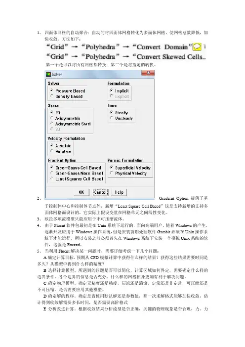
1、四面体网格的自动聚合:自动的将四面体网格转化为多面体网格,使网格总数降低,加快收敛。
方法如下:第一个是可以将所有网格都转换;第二个是将指定的转换。
2、Gradient Option 提供了基于控制体中心和控制体节点外,新增“Least Square Cell Based”这是支持新增的支持多面体网格而设计的,它实际上假设变量在网格单元之间线性变化。
3、欧拉多项流模型只能应用于不可压缩流体。
4、由于Fluent软件包最初是在Unix系统下运行的,面向高端用户,随着Windows的产生,逐渐开发应用于Windows操作系统,但是安装前期处理软件Gambit必须在Unix操作系统下才能运行,所以安装之前必须首先在Windows系统下安装一个模拟Unix系统的软件,这就是Exceed。
5、当利用Fluent解决某一问题时,需要详细考虑一下几个问题:A确定计算目标。
预期从CFD模拟计算中获得什么样的结果?获得这些结果需要时间是多久?从模型中得到什么样的精度?B选择计算模型。
所遇到的问题是否可以简化,计算区域如何界定,需要确定什么样的边界条件,各个边界的信息是否充分,什么样的网格拓扑更加有利于解决问题。
C确定物理模型。
确定无粘度还是粘度,层流还是湍流,定常还是非定常,可压缩还是不可压缩,是否需要应用其他模型。
D确定解的程序。
确定是否使用默认解还是参数值,那一次求解格式能够加快收敛,估计得到收敛解需要多长时间,是否需要高阶格式E分析改进计算。
根据收敛结果分析流型是否正确,关键的物理现象是否合理,力、力矩、流量、温度等与实验值比较是否满足实验精度,是否需要做模型方面的改进,计算域是否需要扩大,边界层网格是否需要加密。
6、Re=ρνr/u根据所给参数,计算出雷诺数来确定层流还是湍流。
7、在命令中输入Reset表示可清空此次任务以前的所有操作,从新开始建立模型。
8、Label选项域表示我们为创建的点或者直线起的名字,有利于命名点不至于乱,在视图控制面板中,选择Label小方框选中,就可以将点的名称显示出来。
矿产资源开发利用方案编写内容要求及审查大纲
矿产资源开发利用方案编写内容要求及《矿产资源开发利用方案》审查大纲一、概述
㈠矿区位置、隶属关系和企业性质。
如为改扩建矿山, 应说明矿山现状、
特点及存在的主要问题。
㈡编制依据
(1简述项目前期工作进展情况及与有关方面对项目的意向性协议情况。
(2 列出开发利用方案编制所依据的主要基础性资料的名称。
如经储量管理部门认定的矿区地质勘探报告、选矿试验报告、加工利用试验报告、工程地质初评资料、矿区水文资料和供水资料等。
对改、扩建矿山应有生产实际资料, 如矿山总平面现状图、矿床开拓系统图、采场现状图和主要采选设备清单等。
二、矿产品需求现状和预测
㈠该矿产在国内需求情况和市场供应情况
1、矿产品现状及加工利用趋向。
2、国内近、远期的需求量及主要销向预测。
㈡产品价格分析
1、国内矿产品价格现状。
2、矿产品价格稳定性及变化趋势。
三、矿产资源概况
㈠矿区总体概况
1、矿区总体规划情况。
2、矿区矿产资源概况。
3、该设计与矿区总体开发的关系。
㈡该设计项目的资源概况
1、矿床地质及构造特征。
2、矿床开采技术条件及水文地质条件。
栅格数据与矢量数据栅格数据结构基于栅格模型的数据结构简称栅格数据结构,是指将空间分割成有规则的网格,称为栅格单元,在各个栅格单元上给出出相应的属性值来表示地理实体的一种数据组织形式。
栅格数据结构表示的是二维表面上的要素的离散化数值,每个网格对应一种属性。
网格边长决定了栅格数据的精度。
矢量数据结构矢量数据结构是利用欧几里得几何学中的点、线、面及其组合体来表示地理实体的空间分布的一种数据组合方式。
矢量与栅格数据结构的比较矢量数据结构的优缺点:优点为数据结构紧凑、冗余度低,有利于网络和检索分析,图形显示质量好、精度高;缺点为数据结构复杂,多边形叠加分析比较困难。
具体来说优点有:1.表达地理数据精度高2.严密的数据结构,数据量小3.用网格链接法能完整地描述拓扑关系,有利于网络分析、空间查询4.图形数据和属性数据的恢复、更新、综合都能实现5.图形输出美观缺点有:1.数据结构较复杂2.软件实现技术要求比较高3.多边形叠合等分析相对困难4.现实和绘图费用高栅格数据的优缺点:优点为数据结构简单,便于空间分析和地表模拟,现势性较强;缺点为数据量大,投影转换比较复杂。
具体来说优点有:1.数据结构相对简单2.空间分析较容易实现3.有利于遥感数据的匹配应用和分析4.空间数据的叠合和组合十分容易方便5.数学模拟方便6.技术开发费用低缺点有:1.数据量较大,冗余度高,需要压缩处理2.定位精度比矢量的低3.拓扑关系难以表达4.难以建立网络连接关系5.投影变形花时间6.地图输出不精美两者比较:栅格数据操作总的来说容易实现,矢量数据操作则比较复杂;栅格结构是矢量结构在某种程度上的一种近似,对于同一地物达到于矢量数据相同的精度需要更大量的数据;在坐标位置搜索、计算多边形形状面积等方面栅格结构更为有效,而且易于遥感相结合,易于信息共享;矢量结构对于拓扑关系的搜索则更为高效,网络信息只有用矢量才能完全描述,而且精度较高。
对于地理信息系统软件来说,两者共存,各自发挥优势是十分有效的。
第17卷第8期2005年8月计算机辅助设计与图形学学报JOURNAL OF COMPU TER 2AIDED DESIGN &COMPU TER GRAPHICSVol 117,No 18Aug 1,2005 收稿日期:2004-03-09;修回日期:2004-07-08 基金项目:国家“八六三”高技术研究发展计划重点项目(2001AA231031,2002AA231021);国家重点基础研究发展规划项目(G1998030608);国家科技攻关计划课题(2001BA904B08);中国科学院知识创新工程前沿研究项目(20006160,20016190(C ))三维网格模型的分割及应用技术综述孙晓鹏1,2) 李 华1)1(中国科学院计算技术研究所智能信息处理重点实验室 北京 100080)2(中国科学院研究生院 北京 100039)(xpsun @ict 1ac 1cn )摘要 对三维网格模型分割的定义、分类和应用情况做了简要回顾,介绍并评价了几种典型的网格模型分割算法,如分水岭算法、基于拓扑和几何信息的分割算法等;同时,对网格分割在几种典型应用中的研究工作进行了分类介绍和评价1最后对三维分割技术今后的发展方向做出展望1关键词 分割Π分解;三维分割;形状特征;网格模型中图法分类号 TP391A Survey of 3D Mesh Model Segmentation and ApplicationSun Xiaopeng 1,2) Li Hua 1)1(Key L aboratory of Intelligent Inf ormation Processi ng ,Instit ute of Com puti ng Technology ,Chi nese Academy of Sciences ,Beiji ng 100080)2(Graduate School of the Chi nese Academy of Sciences ,Beiji ng 100039)Abstract In this paper ,we present a brief summary to 3D mesh model segmentation techniques ,includ 2ing definition ,latest achievements ,classification and application in this field 1Then evaluations on some of typical methods ,such as Watershed ,topological and geometrical !method ,are introduced 1After some ap 2plications are presented ,problems and prospect of the techniques are also discussed 1K ey w ords segmentation Πdecomposition ;3D segmentation ;shape features ;mesh model1 引 言基于三维激光扫描建模方法的数字几何处理技术,继数字声音、数字图像、数字视频之后,已经成为数字媒体技术的第四个浪潮,它需要几何空间内新的数学和算法,如多分辨率问题、子分问题、第二代小波等,而不仅仅是欧氏空间信号处理技术的直接延伸[1]1在三维网格模型已成为建模工作重要方式的今天,如何重用现有网格模型、如何根据新的设计目标修改现有模型,已成为一个重要问题1网格分割问题由此提出,并成为近年的热点研究课题[223]12 网格分割概述三维网格模型分割(简称网格分割),是指根据一定的几何及拓扑特征,将封闭的网格多面体或者可定向的二维流形,依据其表面几何、拓扑特征,分解为一组数目有限、各自具有简单形状意义的、且各自连通的子网格片的工作1该工作被广泛应用于由点云重建网格、网格简化、层次细节模型、几何压缩与传输、交互编辑、纹理映射、网格细分、几何变形、动画对应关系建立、局部区域参数化以及逆向工程中的样条曲面重建等数字几何处理研究工作中[223]1同时,三维网格模型的局部几何拓扑显著性也是对三维网格模型进行检索的一种有效的索引[4]1与网格曲面分割有关、并对其影响巨大的一个早期背景工作是计算几何的凸分割,其目的是把非凸的多面体分解为较小的凸多面体,以促进图形学的绘制和渲染效率1该工作已经有了广泛的研究,但多数算法难以实现和调试,实际应用往往不去分割多面体,而是分割它的边界———多边形网格1多面体网格边界的分割算法有容易实现、复杂形体输出的计算量往往是线性的等优势[5]1另外一个早期背景工作是计算机视觉中的深度图像分割,其处理的深度图像往往具有很简单的行列拓扑结构,而不是任意的,故其分割算法相对简单[6]1三维网格模型的分割算法一般是从上述两类算法推广而来1心理物理学认为:人类对形状进行识别时,部分地基于分割,复杂物体往往被看作简单的基本元素或组件的组合[728]1基于这个原理,Hoffman 等[9]于1984年提出人类对物体的认知过程中,倾向于把最小的负曲率线定义为组成要素的边界线,并据此将物体分割为几个组成要素,即视觉理论的“最小值规则”1由此得到的分割结果称为“有意义的”分割,它是指分割得到的子网格必须具有和其所在应用相关的相对尺寸和组织结构1由于曲率计算方法不同,很多算法给出的有意义的分割结果也存在差异1诸多应用研究[10214]证明,网格模型基于显著性特征的形状分割,是物体识别、分类、匹配和跟踪的基本问题1而有意义的分割对于网格模型显著占优特征的表示和提取、多尺度的存储和传输以及分布式局部处理都是十分有意义的1211 网格分割的发展较早的三维网格分割工作可以追溯到1991年,Vincent 等[15]将图像处理中的分水岭算法推广到任意拓扑连接的3D 曲面网格的分割问题上11992年,Falcidieno 等[16]按照曲率相近的原则,把网格曲面分割为凹面片、凸面片、马鞍面片和平面片11993年,Maillot 等[17]将三角片按法向分组,实现了自动分割;1995年,Hebert 等[18]给出了基于二次拟合曲面片的曲率估计方法,并把区域增长法修改推广应用到任意拓扑连接的网格曲面分割问题中;1995年,Pedersen [19]和1996年Krishnamurthy 等[20]在他们的动画的变形制作过程中,给出了用户交互的分割的方法11997年,Wu 等[3]模拟电场在曲面网格上的分布,给出了基于物理的分割方法;1998年Lee 等[21]和2000年Guskov 等[22]给出了几个对应于简化模型的多分辨率方法;1999年Mangan 等[2]使用分水岭算法实现网格分割,并较好地解决了过分割问题;2001年,Pulla 等[23224]改进了Mangan 的曲率估计工作;1999年,Gregory 等[25]提出一个动画设计中的交互应用,根据用户选择的特征点将网格曲面分割为变形对应片;1999年,Tan 等[26]基于顶点的简化模型建立了用于碰撞检测的、更紧致于网格曲面分割片的层次体包围盒12000年,Rossl 等[27]在逆向工程应用中,在网格曲面上定义了面向曲率信号的数学形态学开闭操作,从而得到去噪后的特征区域骨架,并实现了网格分割;2001年,Yu 等[28]的视觉系统自动将几何场景点云分割为独特的、用于纹理映射和绘制的网格曲面片二叉树;Li 等[29]为了碰撞检测,给出了基于边收缩得到描述几何和拓扑特征的骨架树,然后进行空间扫描自动分割;Sander 等[30]使用区域增长法,按照分割结果趋平、紧凑的原则分割、合并分割片1所有这些方法都是为了使分割的结果便于参数化,即只能产生凸的分割片1由此产生边界不连续的效果12002年,Werghi 等[31]识别三维人体扫描模型的姿态,根据人体局部形状索引进行网格模型的分割;Bischoff 等[32]和Alface 等[33]分别给出了网格分割片光谱在几何压缩和传输中的应用;Levy 等[34]在纹理生成工作中,以指定的法向量的夹角阈值对尖锐边滤波,对保留下来的边应用特征增长算法,最后使用多源Dijkstra 算法扩张分割片实现了网格模型的分割;2003年,Praun 等[35]将零亏格网格曲面投影到球面上,然后把球面投影到正多面体上得到与多面体各面对应的网格模型分割,最后将多面体平展为平面区域以进行参数化,但其结果不是有意义的分割1212 网格分割的分类早期的网格分割算法多为手工分割或者半自动分割,近两年出现了基于自动分割的应用工作1从网格模型的规则性来看,可将分割算法分为规则网格分割、半规则网格分割和任意结构的网格分割算法,根据分割结果可以分为有意义的分割和非有意义的分割1同时,面向不同的应用目标出现了不同的分割策略(见第4节)1目前,网格分割的质量指标主要有三个方面:边界光顺程度、是否有意义、过分割处理效果1多数分8461计算机辅助设计与图形学学报2005年割算法以边界光顺为目标,采用的方法有在三角网格上拟合B样条曲面然后采样[20],逼近边界角点(两个以上分割片的公共顶点)间的直线段[30]等1近年来多数分割算法都追求产生有意义的分割结果1对于过分割的处理方法目前主要有忽略、合并和删除三种方式1多数三维网格分割算法是从二维图像分割的思想出发,对图像分割算法作三维推广得到其三维网格空间的应用1如分水岭算法[2,15,23224,36239]、K2 means算法[40]、Mean2shift算法[41]以及区域增长算法[18,30]等1同样,与图像处理问题类似,光谱压缩[33,42243]、小波变换[31]等频谱信息处理方法在三维网格分割中也有算法1除此之外,同时考虑几何与拓扑信息的分割会产生较好的结果1这方面的工作主要有基于特征角和测地距离度量[44]、基于高斯曲率平均曲率[45247]、基于基本体元[32]、基于Reeb图[48250]、基于骨架提取和拓扑结构扫描[27,29,51252]等使用三维网格曲面形状特征的算法1作为网格模型的基础几何信息,曲率估计方法目前主要为曲面拟合、曲线拟合以及离散曲率等三种1其中曲面拟合法较为健壮,但是计算量大;离散曲率法计算量小,但是除个别算法外都不是很健壮,且无主方向主曲率信息;曲线拟合的曲率估计方法则集中了上述两种方法的优势[3],实际研究中使用较多13 典型三维网格分割算法311 分水岭算法1999年,Mangan等[2]的工作要求输入的是三角网格曲面,以及任何一种可以用来计算每个顶点曲率的附加信息(如曲面法向量等),并针对体数据和网格数据给出了两种曲率计算方法;但是分水岭算法本身和曲率的类型无关1首先,计算每个顶点的曲率(或者其他高度函数),寻找每个局部最小值,并赋予标志,每一个最小值都作为网格曲面的初始分割;然后,开始自下而上或者自上而下地合并分水岭高度低于指定阈值的区域,有时平坦的部分也会得到错误的分割,后处理解决过分割问题1分割为若干简单的、无明确意义的平面或柱面,属于非有意义的分割1Rettmann等[36237]结合测地距离,并针对分水岭算法的过分割给出一个后处理,实现了MRI脑皮层网格曲面的分割12002年,Marty[38]以曲率作为分水岭算法的高度函数,给出了有意义的分割结果1 2003年,Page等[39]的算法同样只分割三角网格,依据最小值规则,他们试图得到网格模型高层描述1其主要贡献为:创建了一个健壮的、对三角网格模型进行分割的贪婪分水岭法;使用局部主曲率定义了一个方向性的、遵循最小值规则的高度图;应用形态学操作,改进了分水岭算法的初始标识集1文献[39]在网格的每一个顶点计算主方向和主曲率,根据曲率阈值,使用贪婪的分水岭算法分割出由最小曲率等高线确定的区域1形态学的开闭操作应用于网格模型每个顶点的k2ring碟状邻域,闭操作会连接空洞,而开操作会消除峡部1创建了标识集后,依据某顶点与其邻接顶点之间的方向,由欧拉公式和已知主曲率计算该顶点在该方向上的法曲率从而得到在该方向上、该顶点与邻接顶点之间的方向曲率高度图,并将其作为方向梯度1对该顶点所在的标识区域使用分水岭算法得到分割片1上述工作表明,分水岭算法在改进高度函数的定义后,可以得到有意义的分割效果1312 基于拓扑信息的网格分割基于几何以及拓扑信息的形状分割方法可以归结为Reeb图[50]、中轴线[52]和Shock图[53254]等1基于拓扑信息的形状特征描述主要有水平集法[55]和基于拓扑持久性的方法[56]11999年,Lazarus等[51]提出从多面体顶点数据集提取轴线结构,在关键点处分割网格的水平集方法,如图1所示1这种轴线结构与定义在网格模型顶点集上的纯量函数关联,称之为水平集图,它能够为变形和动画制作提供整体外形和拓扑信息1图1 人体网格模型及其水平集图文献[51]针对三角剖分的多面体,使用与源点之间的最短路径距离作为水平集函数,基于Dijkstra 算法构造记录水平集图的结构树,其根结点、内部结点和叶子分别表示源点、水平集函数的鞍点和局部最大值点1该工作可以推广到非三角网格模型1 2001年,Li等[29]基于PM算法[57]的边收缩和94618期孙晓鹏等:三维网格模型的分割及应用技术综述空间扫掠,给出了一个有效的、自动的多边形网格分割框架1该工作基于视觉原理,试图将三维物体分割为有视觉意义和物理意义的组件1他们认为三维物体最显著的特征是几何特征和拓扑特征,由此,定义几何函数为扫掠面周长在扫掠结点之间的积分为骨架树中分支的面积;定义拓扑函数为相邻两个扫掠面拓扑差异的符号函数,并定义了基于微分几何和拓扑函数的关键点1文献[29]首先基于PM算法将每条边按照其删除误差函数排序,具有最小函数值的边收缩到边中点,删除其关联的三角形面片;如果某边没有关联任何三角片则指定为骨架边,保持其顶点不变;循环上述过程,得到一个新的、通过抽取给定多边形网格曲面骨架的方法1其次,加入虚拟边连接那些脱节的骨架边,称这些虚拟边以及原有的骨架边组成的树为骨架树,即为扫掠路径1扫掠路径为分段线条1然后,定义骨架树中分支面积(扫掠面周长函数在扫掠结点之间的积分),分支面积较小的首先扫掠,以保证小的、但是重要的分割片被首先抽取出来,以免被其他较大的分割片合并1最后,沿扫掠路径计算网格的几何、拓扑函数的函数值1一旦发现几何函数、拓扑函数的关键点,抽取两个关键点之间的网格曲面得到一个新的分割片1整个过程无需用户干涉12003年,Xiao等[48249]的工作基于人体三维扫描点云的离散Reeb图,给出了三维人体扫描模型的一个拓扑分割方法:通过探测离散Reeb图的关键点,抽取表示身体各部分的拓扑分支,进而进行分割1水平集法具有较高的计算速度和健壮的计算精度1基于拓扑持久性的方法结合代数学,能更准确地计算形状特征,但是没有解决分割问题[55256]1 313 基于实体表示的网格分割2002年,Bischoff等[32]把几何形状分割为表示其粗糙外形的若干椭球的集合,并附加一个独立的网格顶点的采样集合来表示物体的细节1生成的椭球完全填充了物体的内部,采样点就是原始的网格顶点1该方法的步骤如下:Step11首先,在物体原始网格的每一顶点上生成一个椭球,或者随机在物体原始网格上采样选择种子点;每个种子点作为球面上的一个顶点,沿该点的网格法向做球面扩展,直至与网格上另外一个顶点相交;然后沿此两点的垂直方向将球面扩张为最大椭球,直至与第三个网格顶点相交;最后沿此三点平面的法向(即该三点所在平面的柱向)扩张,直至与第四个网格顶点相近,由此得到一个椭球1Step21对生成的椭球进行优化选择,体积最大的椭球首先被选中,以后每一次都将选出对累计体积贡献最大的椭球1如果有若干体积累计贡献相近的椭球同时出现的情况发生,则最小半径最短的椭球被选出1为了简化体积累计贡献的计算,对椭球体素化后计算完全包含在椭球内的体素的数目进行堆排序1发送方传送选出的椭球集合;接收方得到包含基本几何和拓扑信息的椭球集合后,使用Marching Cubes算法或者Shrink2wrapping算法抽取0等值面1显然即使部分椭球丢失,工作依然可以继续:因为椭球是互相重叠的,抽取等值面不影响它们的拓扑关系,而且如果重叠充分,丢失少部分椭球不会影响重要形状信息的重构1如图2所示1图2 以不同数目椭球表示的网格分割Step31在生成很好地逼近原始物体的初始网格后,开始将采样点(即原始网格顶点)插入网格[58]1为了提高最终重构结果的质量,由Marching Cubes算法生成的临时网格顶点在网格原始顶点陆续到来后,最终被删除,因为它们不是物体的原始顶点1314 基于模糊聚类的层次分解2003年,Katz等[44]提出了模糊聚类的层次分解算法,算法处理由粗到精,得到分割片层次树1层次树的根表示整个网格模型S1在每个结点,首先确定需要进一步分割为更精细分割片的数目,然后执行一个k2way分割1如果输入的网格模型S由多个独立网格构成,则分别对每个网格进行同样的操作1分割过程中,算法不强调每个面片必须始终属于特定的分割片1大规模网格模型的分割在其简化模型上进行,然后将分割片投影到原始网格模型上,在不同的尺度下计算分割片之间的精确边界1文献[44]算法优点是:可以对任意拓扑连接的或无拓扑连接的、可定向的网格进行处理;避免了过分割和边界锯齿;考虑测地距离和凸性,使分割边界通过凹度最深的区域,从而得到有意义的分割结果1分割结果适用于压缩和纹理映射14 三维网格分割应用411 三维检索中的网格分割算法在三维VRML数据库中寻找一个与给定物体0561计算机辅助设计与图形学学报2005年相似的模型的应用需求,随着WWW的发展正变得越来越广泛,如计算生物学、CAD、电子商务等1形状描述子和基于特征的表示是实体造型领域中基本的研究问题,它们使对物体的识别和其他处理变得容易1因为相似的物体有着相似的分割,所以分割结构形状描述子可以用于匹配算法1中轴线、骨架等网格模型拓扑结构的形状描述子在三维模型检索中也得到研究,它可以从离散的体数据以及边界表示数据(网格模型)中抽取出来1对于后者,目前还没有精确、有效的结果[39]1但我们相信,依据拓扑信息进行分割得到的分布式形状描述子也是一种值得尝试的三维模型检索思路1 2002年,Bischoff等[32]提出从椭球集合中得到某种统计信息,如椭球半径的平均方差或者标准方差,以及它们的比率,由于这些统计信息在不同的形状修改中都保持不变,作为一种检索鉴别的标识的想法1但是没有严格的理论或者实验结果证明1 2002年,Zuckerberger等[59]在一个拥有388个VRML三维网格模型的数据库上,进行基于分割的变形、简化、检索等三个应用1首先将三维网格模型分割为数目不多的有意义的分割片,然后评价每一个分割片形状,确定它们之间的关系1为每个分割建立属性图,看作是与原模型关联的索引,当数据库中检索到与给定网格模型相似的物体时,只是去比较属性图相似的程度1属性图与其三维模型的关联过程分为三步:(1)分割网格曲面为有限数目的分割片;(2)每一个分割片拟合为基本二次曲面形状;(3)依据邻接分割片的相对尺寸关系进行过分割处理,最后构造网格曲面模型的属性图1对分割片作二次拟合,由此产生检索精确性较差的问题;分割片属性图的比较采用图同构的匹配方法,计算量较大,且是一个很困难的问题;从其实验结果看,有意义的分割显然还不够,出现飞机、灯座等模型被检索为与猫相似的结构;区分坐、立不同的人体模型效果显然也很差等12003年,Dey等[4]基于网格模型的拓扑信息,给出了名为“动力学系统”的形状特征描述方法,并模拟连续形状定义离散网格形状特征1实验表明该算法十分有效地分割二维及三维形状特征1他们还给出了基于此健壮特征分割方法的形状匹配算法1 412 几何压缩传输中的网格分割健壮的网格模型压缩传输方法必须保证即使部分几何信息丢失,剩下的部分至少能够得到一个逼近原始物体的重构,即逼近的质量下降梯度,要大大滞后于信息丢失梯度1无论是层次结构的还是过程表示的多边形网格模型,它们的缺陷是:严格的拓扑信息一致性要求1顶点和面片之间的交叉引用导致即使在传输中丢失了1%的网格数据,也将导致无法从99%的剩余信息里重建网格曲面的任何一部分1对此可以考虑引入高度的冗余信息,即使传输中丢失一定额度的数据,接收方依然可以重构大部分的几何信息1问题的关键是将几何体分割为相互独立的大块信息,如单个点,这样接收方可以在不依赖相关索引信息的情况下,重构流形的邻域关系1为了避免接收方从点云重构曲面的算法变得复杂,早期的健壮传输方法总假设至少整体拓扑信息可以无损地传送1一旦知道了粗糙的形状信息,接收方可以插入一些附加点生成逼近网格12002年,Bischoff等[32,58]在网格分割工作中将每个椭球互相独立地定义自己的几何信息1由于椭球的互相重叠,冗余信息由此产生,因此如果只有很少的椭球丢失,网格曲面的拓扑信息和整体形状不会产生变化1冗余信息不会使存储需求增加,因为每个椭球和三角网格中每个顶点一样,只需要9个存储纯量1其传送过程如下:种子点采样生成椭球集合;传送优化选择的椭球子集;接收方抽取等值面重构逼近网格;以陆续到来的原始网格顶点替换临时网格顶点11996年,Taubin等[42]首先在几何压缩处理中提出光谱压缩,其工作在三维网格模型按如下方式应用傅里叶变换:由任意拓扑结构的网络顶点邻接矩阵及其顶点价数,得到网格Laplacian矩阵的定义及由其特征向量构成的R n空间的正交基底,相对应的特征值即为频率1三维网格顶点的坐标向量在该空间的投影即为该网格模型的几何光谱1网格表面较为光顺的区域即为低频信号12000年,Karni等[43]将几何网格分割片光谱推广到传输问题上1光谱直接应用于定义几何网格的拓扑信息时,会产生伪频率信息1对于大规模的网格,由于在网格顶点数目多于1000时,Laplacian矩阵特征向量的计算几乎难以进行,因此该工作在最小交互前提下,将网格模型分割为有限数目的分割片1该方法有微小的压缩损失,且在分割片边界出现人工算法痕迹12003年,Alface等[33]提出了光谱表示交叠方法:扩张分割片,使分割片之间产生交叠1具体方法是把被分割在其他邻接分割片中的、但与该分割片15618期孙晓鹏等:三维网格模型的分割及应用技术综述邻接的三角片的顶点,按旋转方向加入到该分割片中,从而由于分割片重叠搭接产生冗余信息,并称这种分割片扩展冗余处理的光谱变换为交叠的正交变换1该工作在几何网格压缩和过程传输的应用中明显地改进了Karni等的工作1显然上述工作的基础是良好的网格分割1建立分片独立的基函数将使得分割效果更为理想1413 纹理贴图中的网格分割如果曲面网格的离散化是足够精细的,如细分网格,那么直接对顶点进行纹理绘制就足够了;否则就要把网格模型分割为一组与圆盘同胚的、便于进行参数化的分割片,再对每片非折叠的分割片参数化,最后分割片在纹理空间里拼接起来1网格模型的分割显然会因其局部性而降低纹理映射纹理贴图、网格参数化的扭曲效果1面向纹理的分割算法一般要求满足两个条件:(1)分割片的不连续边界不能出现人工算法痕迹;(2)分割片与圆盘同胚,而且不引入太大的变形就可以参数化1不要求有意义的分割结果12001年,Sander等[30]基于半边折叠的PM算法,使用贪婪的分割片合并方法(区域增长法)对网格模型进行分割1首先将网格模型的每一个面片都看作是独立的分割片,然后每个分割片与其邻接分割片组对、合并1在最小合并计算量的前提下,循环执行分割片对的合并操作,并更新其他待合并分割片的计算量1当计算量超出用户指定的阈值时,停止合并操作1分割片之间的边界为逼近角点间直线段的最短路径,从而减轻了锯齿情况12002年,Levy等[34]将网格模型分割为具有自然形状的分割片,但仍然没有得到有意义的分割结果1为了与圆盘同胚,该算法自动寻找位于网格模型高曲率区域的特征曲线,避免了在平展区域内产生分割片边界,并增长分割片使他们在特征曲线上相交,尽量获得尺寸较大的分割片1414 动画与几何变形中的网格分割影视动画制作中,多个对象间的几何变形特技使用基于网格分割的局部区域预处理1如建立动画区域对应关系,对多个模型进行一致分割,然后在多个模型的对应分割片之间做变形,将提高动画制作的精度和真实性;且每个“Polygon Soup”模型都可用来建立分割片对应;模型间的相似分割有利于保持模型的总体特征1目前,多数的自动对应算法精度较低,手工交互指定对应关系的效率又太低1 1996年,Krishnamurthy等[20]从高密度、非规则、任意拓扑结构的多边形网格出发,手工指定分割边界,构造张量积样条曲面片的动画模型1文献[20]首先在多边形网格的二维投影空间交互选择一个顶点序列,然后自动地将顶点序列关联到网格上最近的顶点上;对于序列中前后两个顶点计算在网格曲面上连接它们的最短路径;对该路径在面片内部进行双三次B样条曲面拟合、光顺、重新采样,得到分割片在两个顶点之间的边界曲线1但计算量的付出依然是非常昂贵的11999年,Gregory等[25]在两个输入的多面体曲面上交互选择多面体顶点,作为一个对应链的端点,对应链上其他顶点通过计算曲面上端点对之间的最短路径上的顶点确定,由此得到这些顶点和边构成的多面体表面网格的连通子图;然后将每一个多面体分割为相同数目的分割片,每个分割片都与圆盘同胚;在分割片之间建立映射、重构、局部加细,完成对应关系的建立;最后插值实现两个多面体之间的变形12002年,Shlafman等[40]的工作不再限制输入网格必须是零亏格或者是二维流形1该算法通过迭代,局部优化面片的归属来改进某些全局函数,因此与图像分割K2means方法相近,属于非层次聚类算法1最终分割片的数目可以由用户预先指定,从而避免了过分割,且适用于动画制作的需求1分割过程的关键在于确认给定的两个面片是否属于同一个分割片1其分割工作是非层次的,因为面片可能会在优化迭代中被调整到另外一个分割片去1该工作表明,基于分割的变形对于保持模型的特征有着重要的意义1局部投影算法能够产生精细的对应区域,且能自动产生有意义的分割片1415 模型简化中的网格分割网格简化是指把给定的一个有n个面片的网格模型处理为另一个保持原始模型特征的、具有较少面片、较大简化Π变形比的新模型1三维网格分割显然可以被看作是一种网格简化,其基本思想是在简化中增加一个预处理过程,先按模型显著特征将其分割为若干分割片,然后在每个分割片内应用简化算法,由此保持了模型的显著特征,如特征边、特征尖锐以及其他精细的细节1例如,把曲率变化剧烈的区域作为分割边界,将曲率变化平缓的区域各自分割开来,就是基于曲率阈值的网格简化方法1网格曲面分割结果的分割片数目在去除过分割后被限制在指定的范围内12561计算机辅助设计与图形学学报2005年。
Applications Of Transformation Of Structured ToUnstructured MeshesLiu Jing1, 2,Zhang Min1,John C. Chai2,Xu Bin11School of Power Eng.,Nanjing University of Science & Technology,Nanjing (210094)2School of Mechanical and Aero spacing Eng.,Nanyang Tech. University,Singapore (639798)E-mail:mz2455@AbstractThe transformation of structured meshes to unstructured meshes is a branch of mesh generation technology. We can obtain the advantages of both grids that structure grids have the characteristics of convergence quickly and unstructured grids have the characteristics of matching sophisticated calculating domains well from this conversion. Meanwhile, it is expanding the widespread useful application of unstructured mesh codes. This paper gave the models of the transformations of the orthogonal meshes and body-fitted meshes. And, the heat conduction equation was solved using the based cell finite volume method and the secondary order accuracy. Finally, a couple of three dimension examples of heat transfer that included different geometries and boundary conditions were given. Therefore, the procedure was validated exactly and actually.Keywords:structured grids/meshes,unstructured grids/meshes,heat conduction1.IntroductionThe first step of numerical simulation is mesh generation that is cutting the continuous computational space into subdomains and identifying each node. The accuracy and efficiency of engineering numerical simulation mainly defend on the meshes and algorisms. In generally, all kind of mesh has its advantages and disadvantages; also the every numerical method has its constraints. Therefore, successful numerical simulation can only be done on the conditions that meshes and algorisms match perfectly [1].Two commonly kinds of mesh are structured and unstructured mesh/grid. The former characteristic is that the relationship between nodes is fixed and implied in the mesh. Thus, no special action is needed to ensure the relationship. But there don’t exists the property in unstructured mesh, so we must store the information about nodes such as volume nodes number, interfaces nodes number, and neighbor volume number[2-4] .It is stubborn to compare structured grid and unstructured grid exactly, besides considering the numerical algorism. In the brief, structured mesh has the good feature, simplex in generating, converging fast, and steady etc, while unstructured mesh can be more applicable for irregular domain, decomposing and encrypting in whole or part domain and used widely in later computation[4] . The paper takes advantage of two kinds of mesh to get fine results by the transformation between them.2.Transformation Between Both MeshesRegular structured mesh in orthogonal coordination is the oldest, most basic and simplex generation technique, including rectangle mesh of Cartesian coordinates and curve mesh in cylindrical coordinates or spherical coordinates. No detail about this kind of mesh, but the paper based on orthogonal mesh and body-fitted grid.First, we have to get the grid nodes of coordination in three dimensions, and then transform them to unstructured grid nodes number. Finally, numerical simulation will be done based on the unstructured mesh. For the transformation, at first, select cells shape and nodes NCTYPE(I) and NCNODE(J,I), here they are vertex number and coordination value (X(I),Y(J),Z(K)) of cell, respectively. Secondly, get the surface information NFTYPE (I) and NFNODE (J, I) of the cells. Where, the node order conform right hand rule, which is, ensuring the direction of surface normal is outside the cells.At the end, storing all neighbor cells information and their boundary property by KBCC (I).Ultimately, we can obtain the six data files. It is exactly these files comprise surfaces and nodes number for every cell and surface. The key of transformation is rearranging the I/J/K order of structured grid nodes to cell series data structure. Although the program is easy to do, the technique proved to be a handicap. Next part program is given in two dimensions.C**************************************************COME HERE FOR THE NODES OF CELL (cell_node.dat)LM=L2*M2 I0=0 J0=0DO 30 I=1,NCV NCTYPE(I)=8 NCNODE(1,I)=I+I0+J0NCNODE(2,I)=I+1 +I0+J0 NCNODE(3,I)=I+L1+I0+J0 NCNODE(4,I)=I+L2+I0+J0 NCNODE(5,I)=I+I0+J0+LMNCNODE(6,I)=I+1 +I0+J0+LM NCNODE(7,I)=I+L1+I0+J0+LM NCNODE(8,I)=I+L2+I0+J0+LM IF(MOD(I,L3).EQ.0) I0=I0+1IF(MOD(I,L3*M3).EQ.0) J0=J0+L230 CONTINUEC**************************************************The particular examples and their results analysis are provided in following paragraphs.3. Heat Conduction ExamplsProblem 1: We have heat transfer conduction without heat source in cubic region. Geometry and computational grids are showed in figure1, and governing equation is heat conduct equation with constant property in three Cartesian coordinates. The left surface has higher temperature T 2, and the left five ones have lower temperature T 1. Arithmetic formula of governing function and boundary conditions are:0=⎟⎠⎞⎜⎝⎛∂∂∂∂+⎟⎟⎠⎞⎜⎜⎝⎛∂∂∂∂+⎟⎠⎞⎜⎝⎛∂∂∂∂z T k z y T k y x T k x(1.1) 0.1,0.1,0.0,0.121======k T T c b a(1.2)(a) Cubic V olume (b) Orthogonal meshes (c) Body-fitted meshesFigure 1 Geometry and structured/unstructured meshesWe can obtain the exact solution of (1.1) and (1.2) (Kakac and Yener, 1993)[5],[][]∑∑∞=∞=−−−−−=−−=11121sinh )(sinh )sin()sin(])1(1[])1(1[4),(),(m n mn mn m n m mn nb y b z x ac T T T y x T y x ααβλβλθ(1.3)Where,n λa n π=(n = 1, 2,…,i ) =m βcm π (m = 1, 2, …,i )22mn mn βλα+=(1.4)In Figure 2, the results of temperature distributions were from the transformation of orthogonalmeshes to unstructured grids. The same one was from the transformation of body-fitted meshes to unstructured grids in Figure 3. The solid lines stand for the exact solution. The dashed lines represent numerical solution. The numbers of grid are 10*10*10. There are agreements of temperature fields in both meshes.(a) X =0.5 (b) Y =0.2 (c) Z =0.5Figure 2. The temperature field of orthogonal meshes(————Exact Solution - - - - - -Numerical Solution)(a) X =0.5 (b) Y =0.2 (c) Z =0.5Figure 3. The temperature field of body-fitted meshesProblem 2: We have heat transfer conduction within heat source in cubic region. Geometry and computational grids are showed in figure1, and governing equation is heat conduct equation with constant property in three Cartesian coordinates as following. The all surfaces maintain the constant temperature (T 1 =0) same as the first kind of boundary condition. Mathematical formula of governing function and boundary conditions are:=∂∂+∂∂+∂∂222222zT y T x T )sin()sin()(1c z a x b y y k ππ−− (2.1)The exact solution of this problem is [6],)sin()sin()sin(]1()()1[(1π8),,,5,3,1222352c z b y n a x cb n a n kb z y x T n πππ⋅++−=∑∞=L ( (2.2)The results of temperature distributions were from the transformation of body-fitted meshes tounstructured grids in Figure 4. The solid lines stand for the exact solution. The dashed lines represent numerical solution. The numbers of grid are 10*10*10. There are agreements of temperature fields in both meshes. There are the symmetrical temperature distribution basic of the boundary conditions and geometry.(a) X =0.5 (b) Y =0.5 (c) Z =0.5Figure 4. The temperature field of body-fitted meshesProblem 3: We have heat transfer conduction without heat source in cylindrical region. Geometry and computational grids are showed in figure 5a, and governing equation is heat conduct equation with constant property in three cylindrical coordinates as following. The outside surface has higher temperature T 2, and the inside surface has lower temperature T 1. Mathematical formula of governing function and boundary conditions are:0112=⎟⎠⎞⎜⎝⎛∂∂∂∂+⎟⎟⎠⎞⎜⎜⎝⎛∂∂∂∂+⎟⎠⎞⎜⎝⎛∂∂∂∂z T k z T k r r T kr r r ϕϕ(3.1) 0.1,0.8,0.4,0.2,0.12121=====k T T r r r r(3.2)The exact solution of this problem is [7-8],)/ln()/ln()/ln()(122211r r r r T r r T r T r r −=(3.3)In Figure 5, the results of temperature distributions were from the transformation of body-fittedmeshes to unstructured grids. The solid lines stand for the exact solution. The dashed lines represent numerical solution. The numbers of grid are 10*10*10. There are agreements of temperature fields in both meshes. There are the symmetrical temperature distribution basic of the boundary conditions and geometry.(a) Meshes (b)Temperature fields in Z=0.5 (c) The flood picture of temperatureFigure 5. The temperature field of cylindrical coordinates4.Closure RemarkThe produces, which the heat conduction equations were solved, was presente d using the unstructured meshes that were transformed from structured grids. There are two kinds of meshes including orthogonal and body-fitted meshes. We show three examples for evaluating and proving this processor accruable and reasonable. The problem one and two are in the Cantinas coordinate and the problem three is in cylindrical coordinate. All results of numerical simulation were compared with the exact solutions. As a result, there is a perfect agreement between them.References[1] 陶文铨. 计算传热学的近代发展[M] 北京: 科学出版社, 2001.[2] PA TANKAR S V. Computation of Conduction and Duct Flow Heat Transfer [M].USA: Innovative Research Inc, 1991.[3] PA TANKAR S V. Numerical Heat Transfer and Fluid Flow [M]. New York: Hemisphere Publishing, 1981.[4] ZHANG M. Modeling of Radiative Heat Transfer and Diffusion Processes Using Unstructured Grid [D]. USA: Tennessee Technological University; 2000.[5] KAKAC S, YENER Y. Heat Conduction (Third edition) [M]. Taylor & Francis, Publisher, 1993.[6] 马信山. 电磁场基础[M]. 北京: 清华大学出版社, 1995.[7] M. N. 奥齐西克. 热传导[M]. 俞昌铭, 译. 北京: 高等教育出版社, 1984.[8] 南京工学院数学教研组. 数学物理方程和特殊函数[M]. 北京: 人民教育出版社, 1982.。