matlab实验指导解读
- 格式:doc
- 大小:177.73 KB
- 文档页数:19

实验1 熟悉软件环境和基本的操作一、实验目的熟悉MATLAB运行环境和了解基本操作。
二、实验内容MATLAB的启动、操作界面组成1.熟悉MATLAB图形界面打开MATLAB,单击命令窗口菜单栏中的各个下拉菜单按钮,试使用各个按钮引出的选项;把光标移动到工具栏中各个图标上(不要按下),查看它们与菜单选项的对应情况。
2.熟悉MATLAB的基本命令。
在命令窗口中分别键入以下内容,以建立若干变量:A=[1 2;3 4;5 6]B=[7,8,9;10,11,12]C=[5 6 7;1 8 3];D=B+C问题1:如何输入一个矩阵变量的行元素和列元素?问题2:观察每行命令后是否加“;”,对显示执行结果有什么区别?键入以下命令或执行操作,查看效果,并体会命令功能:(1)工作空间管理。
whowhosclear A(2)路径编辑。
试用菜单File/Set Path将D盘根目录及其下的所有子目录和文件夹包含进来,设为搜索路径。
问题3:当前路径是什么?问题4:搜索路径是什么意思?(3)联机帮助help pausehelpwin(4)窗口清理。
先画出正弦函数在0-2π之间的图形,再用以下各种窗口清理命令,看每项命令都清除了什么。
figureplot(sin(0:0.1:6.28))claclfclose注意:figure为打开一幅图形图像窗口close为关闭当前图形图像窗口,而close all为关闭所有已打开的图形图像窗口。
(5)MATLAB基本矩阵操作演示playshow intro(6)MATLAB图形绘制演示playshow buckydem(7)MATLAB数学功能演示(快速傅氏变换)playshow fftdemo(8)MATLAB三维造型演示(茶壶演)playshow teapotdemo3.打开MATLAB命令窗口,键入demos,观看演示程序。
三、思考题1.将pi分别用15位数字格式、分数格式、十六进制格式、5位数字的科学计数法显示。

2015/2016学年下学期《信号与系统》实验报告班级:学号:学生姓名:指导教师:2016年3月8 日实验一 基本函数仿真实验项目: 基本函数仿真实验时间: 2016年 3 月 8 日 星期 二 第 34 节课 实验地点: 1501实验室 实验目的:1、 学习使用MATLAB 软件2、 学习MATLAB 中各种函数,并应用函数分析3、 对MATALB 的进一步的学习了解,熟练掌握MATALB 的各种操纵,学会使用MATALB 解决复杂的运算并学会用MATALB 解决平时学习4、 了解MATALB 的数值运算5、 了解MATALB 的基本函数和命令6、 学习掌握MATALB 有关命令 实验内容: 1、(1) 题目:应用MA TLAB 方法实现单位阶跃信号和矩形脉冲。
(2) 程序清单(源程序)解:对于阶跃函数,MATLAB 中有专门的stairs 绘图命令。
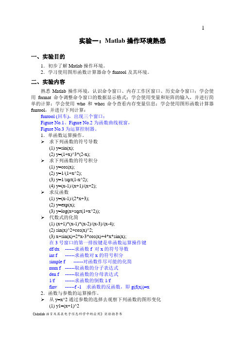
例如,实现)(t 和矩形脉冲的程序如下:t=-1:2; % 定义时间范围向量t x=(t>=0);subplot(1,2,1),stairs(t,x);axis([-1,2,-0.1,1.2]); grid on % 绘制单位阶跃信号波形 t=-1:0.001:1; % 定义时间范围向量t g=(t>=(-1/2))-(t>=(1/2));subplot(1,2,2),stairs(t,g);axis([-1,1,-0.1,1.2]); grid on % 绘制矩形脉冲波形(3) 运行结果(截图)00.20.40.60.8100.20.40.60.81图1 例1图(4)函数解析Subplot:使用方法:subplot (m,n,p )或者subplot (m n p )。
是将多个图画到一个平面上的工具。
其中,m 表示是图排成m 行,n 表示图排成n 列,也就是整个figure 中有n 个图是排成一行的,一共m 行,如果m=2就是表示2行图。

MATLAB基础实验指导书漳州师范学院物电系2010年10月目录实验一MATLAB环境的熟悉与基本运算 (2)实验二MATLAB数值运算 (8)实验三MATLAB语言的程序设计 (12)实验四MATLAB的图形绘制 (16)实验五采用SIMULINK的系统仿真 (20)实验六MATLAB在电路中的应用 (25)实验七MATLAB在信号与系统中的应用 (27)实验八MATLAB在控制理论中的应用 (29)实验一 MATLAB环境的熟悉与基本运算一、实验目的:1.熟悉MATLAB开发环境2.掌握矩阵、变量、表达式的各种基本运算二、实验基本知识:1.熟悉MATLAB环境:MATLAB桌面和命令窗口、命令历史窗口、帮助信息浏览器、工作空间浏览器文件和搜索路径浏览器。
2.掌握MATLAB常用命令3.MATLAB变量与运算符变量命名规则如下:(1)变量名可以由英语字母、数字和下划线组成(2)变量名应以英文字母开头(3)长度不大于31个(4)区分大小写MATLAB中设置了一些特殊的变量与常量,列于下表。
MATLAB运算符,通过下面几个表来说明MATLAB的各种常用运算符表2 MATLAB算术运算符表3 MATLAB关系运算符表4 MATLAB逻辑运算符表5 MATLAB特殊运算4.MATLAB的一维、二维数组的寻访表6 子数组访问与赋值常用的相关指令格式5.MATLAB的基本运算表7 两种运算指令形式和实质内涵的异同表6.MATLAB的常用函数表8 标准数组生成函数表9 数组操作函数三、实验内容1、学习使用help命令,例如在命令窗口输入help eye,然后根据帮助说明,学习使用指令eye(其它不会用的指令,依照此方法类推)2、学习使用clc、clear,观察command window、command history和workspace等窗口的变化结果。
3、初步程序的编写练习,新建M-file,保存(自己设定文件名,例如exerc1、exerc2、exerc3……),学习使用MATLAB的基本运算符、数组寻访指令、标准数组生成函数和数组操作函数。
实验一:Matlab操作环境熟悉一、实验目的1.初步了解Matlab操作环境。
2.学习使用图形函数计算器命令funtool及其环境。
二、实验内容熟悉Matlab操作环境,认识命令窗口、内存工作区窗口、历史命令窗口;学会使用format命令调整命令窗口的数据显示格式;学会使用变量和矩阵的输入,并进行简单的计算;学会使用who和whos命令查看内存变量信息;学会使用图形函数计算器funtool,并进行下列计算:funtool (回车),出现三个窗口:Figure No.1、Figure No.2为函数曲线视窗,Figure No.3为运算控制器。
1.单函数运算操作。
求下列函数的符号导数(1) y=sin(x);(2) y=(1+x)^3*(2-x);求下列函数的符号积分(1) y=cos(x);(2) y=1/(1+x^2);(3) y=1/sqrt(1-x^2);(4) y=(x-1)/(x+1)/(x+2);求反函数(1) y=(x-1)/(2*x+3);(2) y=exp(x);(3) y=log(x+sqrt(1+x^2));代数式的化简(1) (x+1)*(x-1)*(x-2)/(x-3)/(x-4);(2) sin(x)^2+cos(x)^2;(3) x+sin(x)+2*x-3*cos(x)+4*x*sin(x);在3号窗口的第一排按键是单函数运算操作键df/dx ------求函数f 对x的符号导数int f ------求函数对x的符号积分simple f ------对函数作尽可能的化简num f ------取函数的分子表达式den f ------取函数的分母表达式1/f ------求函数的倒数1/ffinv ------f -1 求函数的反函数,即g(f(x))=x2.函数与参数的运算操作。
从y=x^2通过参数的选择去观察下列函数的图形变化(1) y1=(x+1)^2(2) y2=(x+2)^2(3) y3=2*x^2(4) y4=x^2+2(5) y5=x^4(6) y6=x^2/2在3号窗口的第二排按键是函数与参数的运算操作键f+a -------求函数与a的和f-a -------求函数与a的差f*a -------求函数与a的积f/a -------求函数除与a的商f^a -------求函数以a为指数的值f(x+a) -------作自变量的变换,以x+a代替xf(x*a) -------作自变量的变换,以a*x代替x其中a的默认值为1/2,可以在控制栏中去修改参数a的数值。

MATLAB语言及应用实验指导书机械与电气工程学院黄高飞余群编写目录实验一基础准备及入门(2学时,验证性) (1)实验二符号计算(2学时,验证性) (5)实验三数值数组及其运算(4学时,验证性) (6)实验四数据和函数的可视化(2学时,验证性) (9)实验五MATLAB语言的程序设计(4学时,综合性) (11)实验六SIMULINK交互式仿真集成环境(2学时,验证性) (14)实验一基础准备及入门一、实验目的1、了解MATLAB操作桌面的基本结构和组成;2、理解Command Window指令窗的作用,掌握指令窗的操作方式和指令的基本语法;3、了解Command History历史指令窗的作用、历史指令的再运行方法;4、理解Current Directory当前路径、搜索路径的作用,掌握当前路径、搜索路径的设置方法;5、理解Workspace Browser工作空间浏览器的作用,掌握内存变量的查阅、删除、保存和载入的基本方法;6、了解Launch Pad的作用;7、掌握M脚本文件的编写、运行方法;8、掌握利用帮助系统查询函数等基本信息的方法。
二、实验原理1、MATLAB操作桌面的基本结构和组成了解MATLAB的基本组件是正确使用MATLAB的基本前提。
MATLAB由以下基本组件组成:(1)指令窗Command Window:可键入各种送给MATLAB运作的指令、函数、表达式;显示除图形外的所有运算结果(2)历史指令窗Command History:记录已经运作过的指令、函数、表达式;(3)当前目录浏览器:进行当前目录的设置;展示相应目录上的M、MDL等文件;(4)工作空间浏览器Workspace Browser:列出MATLAB工作空间中所有的变量名、大小、字节数;(5)内存数组编辑器Array Editor:在工作空间浏览器中对变量进行操作时启动(6)开始按钮(7)交互界面分类目录窗Launch Pad:以可展开的树状结构列着MATLAB提供的所有交互界面(8)M文件编辑/调试器(9)帮助导航/浏览器2、MATLAB指令窗的基本操作MATLAB指令窗给用户提供了最直接的交互界面,可用于输入和执行指令、显示指令运行结果、调试MATLAB程序等常用的MATLAB仿真计算功能。

MATLAB实验指导书(DOC)MATLAB实验指导书前⾔MATLAB程序设计语⾔是⼀种⾼性能的、⽤于科学和技术计算的计算机语⾔。
它是⼀种集数学计算、分析、可视化、算法开发与发布等于⼀体的软件平台。
⾃1984年MathWorks公司推出以来,MATLAB以惊⼈的速度应⽤于⾃动化、汽车、电⼦、仪器仪表和通讯等领域与⾏业。
MATLAB有助于我们快速⾼效地解决问题。
MATLAB相关实验课程的学习能加强学⽣对MATLAB程序设计语⾔理解及动⼿能⼒的训练,以便深⼊掌握和领会MATLAB应⽤技术。
⽬录基础型实验............................................................................................ - 1 - 实验⼀MATLAB集成环境使⽤与基本操作命令练习............. - 1 - 实验⼆MATLAB中的数值计算与程序设计 ............................. - 7 - 实验三MATLAB图形系统......................................................... - 9 -基础型实验实验⼀ MATLAB 集成环境使⽤与基本操作命令练习⼀实验⽬的熟悉MATLAB 语⾔编程环境;熟悉MATLAB 语⾔命令⼆实验仪器和设备装有MATLAB7.0以上计算机⼀台三实验原理MATLAB 是以复杂矩阵作为基本编程单元的⼀种程序设计语⾔。
它提供了各种矩阵的运算与操作,并有较强的绘图功能。
1.1基本规则1.1.1 ⼀般MATLAB 命令格式为[输出参数1,输出参数2,……]=(命令名)(输⼊参数1,输⼊参数2,……)输出参数⽤⽅括号,输⼊参数⽤圆括号如果输出参数只有⼀个可不使⽤括号。
1.1.2 %后⾯的任意内容都将被忽略,⽽不作为命令执⾏,⼀般⽤于为代码加注释。
实验一:Matlab操作环境熟悉一、实验目的1.初步了解Matlab操作环境。
2.学习使用图形函数计算器命令funtool及其环境。
二、实验内容熟悉Matlab操作环境,认识命令窗口、内存工作区窗口、历史命令窗口;学会使用format命令调整命令窗口的数据显示格式;学会使用变量和矩阵的输入,并进行简单的计算;学会使用who和whos命令查看内存变量信息;学会使用图形函数计算器funtool,并进行下列计算:1.单函数运算操作。
➢求下列函数的符号导数(1) y=sin(x);(2)y=(1+x)^3*(2-x);➢求下列函数的符号积分(1) y=cos(x);(2) y=1/(1+x^2);(3)y=1/sqrt(1—x^2);(4) y=(x-1)/(x+1)/(x+2);➢求反函数(1) y=(x—1)/(2*x+3);(2) y=exp(x);(3)y=log(x+sqrt(1+x^2));➢代数式的化简(1) (x+1)*(x—1)*(x—2)/(x—3)/(x-4);(2) sin(x)^2+cos(x)^2;(3)x+sin(x)+2*x—3*cos(x)+4*x*sin(x);2.函数与参数的运算操作。
➢从y=x^2通过参数的选择去观察下列函数的图形变化(1)y1=(x+1)^2(2)y2=(x+2)^2(3) y3=2*x^2(4)y4=x^2+2(5)y5=x^4(6)y6=x^2/23.两个函数之间的操作➢求和(1) sin(x)+cos(x)(2) 1+x+x^2+x^3+x^4+x^5➢乘积(1) exp(—x)*sin(x)(2)sin(x)*x➢商(1)sin(x)/cos(x);(2)x/(1+x^2);(3)1/(x-1)/(x-2);➢求复合函数(1) y=exp(u) u=sin(x)(2)y=sqrt(u) u=1+exp(x^2)(3)y=sin(u)u=asin(x)(4) y=sinh(u)u=—x三、设计提示1.初次接触Matlab应该注意函数表达式的文本式描述。
MATLAB基础教程实验指导书实验一:Desktop操作桌面基础一、实验目的及要求1、熟悉MATLAB系统的安装流程,掌握MATLAB的启动和退出。
2、掌握MATLAB系统的各命令窗口的功能,熟悉常用选项和工具栏的功能和用途。
3、熟悉简单程序的输入、运行、调试及结果的显示过程。
二、实验内容1、认识MATLAB集成环境:熟悉个操作窗口的功能和用途。
掌握File(文件)、Edit(编辑)、View(显示)、Web(网络)、Window(窗口)和Help(帮助) 等菜单命令的使用。
2、启动和退出MATLAB(1)启动MATLAB的M文件。
在启动MATLAB时,系统可自动执行主M文件matlabrc.m,在matlabrc.m的末尾还会检测是否存在startup.m,如存在则会自动执行它。
在网络系统中,matlabrc.m保留给系统管理员,而各个用户可利用startup.m进行初始设置。
(2)、终止或退出MATLAB。
quit命令可终止MATLAB,但不保存工作空间的内容。
为保存工作空间的内容,可使用save命令。
1、利用save、load命令,保存和恢复工作空间。
用clear命令可清空工作空间。
(1)、工作空间中的变量可以用save命令存储到磁盘文件中。
(2)、用load命令可将变量从磁盘文件读入MATLAB的工作空间。
(3)、用clear命令可清除工作空间中现存的变量。
4、MATLAB的所有图形工具窗体都可以嵌入MATLAB窗体(Dock),也可以从MATLAB窗体中弹出(Undock),例如在MATLAB默认的图形窗体环境下,单击命令行窗体左上角按钮,就可以将MATLAB命令行窗体弹出。
要求分别将命令行窗体(Command Window)、命令行历史窗体(Command History)、当前路径查看器(Current Directory)、工作空间浏览器(Workspace Browser)、帮助(Help)、MATLAB性能剖析工具(Profiler) 从MATLAB窗体中弹出和嵌入MATLAB窗体(Dock)。
MATLAB实验指导书(共5篇)第一篇:MATLAB实验指导书MATLAB 实验指导书皖西学院信息工程学院实验一 MATLAB编程环境及简单命令的执行一、实验目的1.熟悉MATLAB编程环境二、实验环境1.计算机2.MATLAB7.0集成环境三、实验说明1.首先应熟悉MATLAB7.0运行环境,正确操作2.实验学时:2学时四、实验内容和步骤1.实验内容(1)命令窗口的使用。
(2)工作空间窗口的使用。
(3)工作目录、搜索路径的设置。
(4)命令历史记录窗口的使用。
(5)帮助系统的使用。
(6)了解各菜单的功能。
2.实验步骤(1)启动MATLAB,熟悉MATLAB的桌面。
(2)进入MATLAB7.0集成环境。
(3)在命令窗口执行命令完成以下运算,观察workspace的变化,记录运算结果。
1)(365-52⨯2-70)÷3 2)>>area=pi*2.5^2 3)已知x=3,y=4,在MATLAB中求z:x2y3 z=2(x-y)4)将下面的矩阵赋值给变量m1,在workspace中察看m1在内存中占用的字节数。
⎡162313⎤⎢511108⎥⎥m1=⎢⎢97612⎥⎢⎥414151⎣⎦执行以下命令>>m1(2 , 3)>>m1(11)>>m1(: , 3)>>m1(2 : 3 , 1 : 3)>>m1(1 ,4)+ m1(2 ,3)+ m1(3 ,2)+ m1(4 ,1)5)执行命令>>helpabs 查看函数abs的用法及用途,计算abs(3 + 4i)6)执行命令>>x=0:0.1:6*pi;>>y=5*sin(x);>>plot(x,y)7)运行MATLAB的演示程序,>>demo,以便对MATLAB有一个总体了解。
五、思考题1、以下变量名是否合法?为什么?(1)x2(2)3col(3)_row (4)for2、求以下变量的值,并在MATLAB中验证。
MATLAB实验指导书指导老师许承东实验一MATLAB基本操作实验目的1、熟悉MATLAB的工作环境;2、掌握MATLAB常用的操作运算符和一些基本操作;3、学会编写M文件。
实验内容e sin3t,其中t的取值范围为[0,4π]。
1、绘制衰减图线y=5.2/t(1)启动MATLAB,如图1.1所示。
图1.1 MATLAB的工作环境(2)直接在命令窗口输入以下代码:(3)程序执行后显示的衰减振荡曲线如图1.2所示。
图1.2 衰减振荡曲线(4)生成M文件。
在历史命令窗口中选中上面所写代码,单击鼠标右键,在弹出菜单中选择Create M-File菜单项,即可创建为M文件,将文件命名为quxian.m保存。
2、向量化和循环结构的比较(1)从工具栏中单击New M-file图标,或从菜单中选择File/New/M-File创建新的M文件,如图1.3所示。
图1.3 创建新的M文件(2)在M文件编辑器中输入以下代码:(3)保存运行。
将文件名改为vectorize_contrast.m保存。
单击Run 命令或直接按F5执行。
(4)执行结果实验二MATLAB基本图形绘制实验目的1、掌握MATLAB二维图形的绘制;2、掌握MATLAB三维图形的绘制。
实验内容1、二维图形的绘制(1)从工具栏中单击New M-file图标,或从菜单中选择File/New/M-File创建新的M文件。
(2)在M文件编辑器中输入以下代码:(3)保存运行。
将文件名改为example_plot.m保存。
单击Run命令或直接按F5执行。
(4)二维图形绘制结果如图2.1所示。
图2.1 二维图形绘制结果2、三维曲面绘制(1)从工具栏中单击New M-file图标,或从菜单中选择File/New/M-File创建新的M文件。
(2)在M文件编辑器中输入以下代码:(3)保存运行。
将文件名改为matlab_script.m保存。
单击Run命令或直接按F5执行。
《数字信号处理》MATLAB实验指导实验一:离散时间信号和离散时间系统一、 实验目的:1、 以MA TLAB 为工具学习离散时间信号的图形表示;2、 以课本提供的例程,练习、理解典型离散信号及其基本运算;3、 通过MATLAB 仿真简单的离散时间系统,研究其时域特性;4、 加深对离散系统的差分方程、冲激响应和卷积分析方法的理解。
二、 实验内容:1、 典型序列的产生与显示;2、 序列的简单运算;3、 复合和复杂信号的产生与显示;4、 离散时间系统的仿真:线性和非线性系统、时变和非时变系统的仿真;5、 线性时不变离散时间系统:系统冲激响应、卷积运算、系统的级联、系统的稳定性;三、实验例程:1、 参照课本例程产生下列序列,并用plot 、stem 好人subplot 命令绘出其图形: ①单位取样序列()n δ;②单位阶跃序列()n μ;③矩形序列RN(n),④斜变序列()n n μ。
所需输入的数据是产生序列的长度L 和抽样频率F T 。
% Program P1_1% Generation of a Unit Sample Sequenceclf;% Generate a vector from -10 to 20n = -10:20;% Generate the unit sample sequenceu = [zeros(1,10) 1 zeros(1,20)];% Plot the unit sample sequencestem(n,u);xlabel('Time index n');ylabel('Amplitude');title('Unit Sample Sequence');axis([-10 20 0 1.2]);2、 编写MATLAB 实指数序列程序,% Program P1_3% Generation of a real exponential sequenceclf;n = 0:35; a = 1.2; K = 0.2;x = K*a.^n;stem(n,x);xlabel('Time index n');ylabel('Amplitude');3、编写产生swept frequency sinusoidal 序列的程序。
% Program P1_7% Generation of a swept frequency sinusoidal sequencen = 0:100;a = pi/2/100;b = 0;arg = a*n.*n + b*n;x = cos(arg);clf;stem(n, x);axis([0,100,-1.5,1.5]);title('Swept-Frequency Sinusoidal Signal');xlabel('Time index n');ylabel('Amplitude');grid; axis;>>4、产生正弦振幅调制序列% Generation of amplitude modulated sequenceclf;n = 0:100;m = 0.4;fH = 0.1; fL = 0.01;xH = sin(2*pi*fH*n);xL = sin(2*pi*fL*n);y = (1+m*xL).*xH;stem(n,y);grid;xlabel('Time index n');ylabel('Amplitude');5、用滑动平均滤波器平滑带噪信号,讨论滤波器长度对平滑效果、输出平滑后信号与输入带噪信号之间延时的影响。
% Program P1_5% Signal Smoothing by Averagingclf;R = 51;d = 0.8*(rand(R,1) - 0.5); % Generate random noisem = 0:R-1;s = 2*m.*(0.9.^m); % Generate uncorrupted signalx = s + d'; % Generate noise corrupted signalsubplot(2,1,1);plot(m,d','r-',m,s,'g--',m,x,'b-.');xlabel('Time index n');ylabel('Amplitude');legend('d[n] ','s[n] ','x[n] ');x1 = [0 0 x];x2 = [0 x 0];x3 = [x 0 0];y = (x1 + x2 + x3)/3;subplot(2,1,2);plot(m,y(2:R+1),'r-',m,s,'g--');legend( 'y[n] ','s[n] ');xlabel('Time index n');ylabel('Amplitude');6、编写输入序列、计算输出序列、差分输出并画出输出序列。
% Program P2_4% Generate the input sequencesclf;n = 0:40; D = 10;a = 3.0;b = -2;x = a*cos(2*pi*0.1*n) + b*cos(2*pi*0.4*n);xd = [zeros(1,D) x];num = [2.2403 2.4908 2.2403];den = [1 -0.4 0.75];ic = [0 0]; % Set initial conditions% Compute the output y[n]y = filter(num,den,x,ic);% Compute the output yd[n]yd = filter(num,den,xd,ic);% Compute the difference output d[n]d = y - yd(1+D:41+D);% Plot the outputssubplot(3,1,1)stem(n,y);ylabel('Amplitude');title('Output y[n]'); grid;subplot(3,1,2)stem(n,yd(1:41));ylabel('Amplitude');title(['Output due to Delayed Input x[n ?', num2str(D),']']); grid; subplot(3,1,3)stem(n,d);xlabel('Time index n'); ylabel('Amplitude');title('Difference Signal'); grid;7、编写输入序列和系统单位脉冲响应的卷积程序并画出图形。
% Program P2_7clf;h = [3 2 1 -2 1 0 -4 0 3]; % impulse response x = [1 -2 3 -4 3 2 1]; % input sequencey = conv(h,x);n = 0:14;subplot(2,1,1);stem(n,y);xlabel('Time index n'); ylabel('Amplitude'); title('Output Obtained by Convolution'); grid; x1 = [x zeros(1,8)];y1 = filter(h,1,x1);subplot(2,1,2);stem(n,y1);xlabel('Time index n'); ylabel('Amplitude'); title('Output Generated by Filtering'); grid;8、编写输入信号经滤波形成的系统输出信号。
% Program P2_9% Generate the input sequenceclf;n = 0:299;x1 = cos(2*pi*10*n/256);x2 = cos(2*pi*100*n/256);x = x1+x2;% Compute the output sequencesnum1 = [0.5 0.27 0.77];y1 = filter(num1,1,x); % Output of System #1 den2 = [1 -0.53 0.46];num2 = [0.45 0.5 0.45];y2 = filter(num2,den2,x); % Output of System #2 % Plot the output sequencessubplot(2,1,1);plot(n,y1);axis([0 300 -2 2]);ylabel('Amplitude');title('Output of System #1'); grid;subplot(2,1,2);plot(n,y2);axis([0 300 -2 2]);xlabel('Time index n'); ylabel('Amplitude'); title('Output of System #2'); grid;9、四、本实验用到的matlab命令Stem plot sin abs cos conv clf subplot filter impz实验二:时域连续时间信号和频域抽样理论的验证与观察一、实验目的:1、理解并掌握信号时域采样和频率抽样理论涉及的过程和效果;2、通过编程加深理解奈奎斯特采样定理,理解不满足采样条件的对时域和频域采样造成的混叠现象。
二、实验内容:1、时域的采样过程、采样定理和混叠效果;2、频域中的采样效果;3、学习buttworth模拟低通滤波器的设计命令;三、实验例程1、连续时间信号的理想抽样及其混叠效果clf;T = 0.4;f = 25;n = (0:T:1)';xs = cos(2*pi*f*n);t = linspace(-0.5,1.5,500)';ya = sinc((1/T)*t(:,ones(size(n))) - (1/T)*n(:,ones(size(t)))')*xs;plot(n,xs,'o',t,ya);grid;xlabel('Time, msec');ylabel('Amplitude');title('Reconstructed continuous-time signal y_{a}(t)');axis([0 1 -1.2 1.2])2、.频率抽样及其混叠效果clf;t = 0:0.002:50;xa = 2*t.*exp(-t);subplot(4,2,1)plot(t,xa);gridxlabel('Time, msec');ylabel('Amplitude');title('Continuous-time signal x_{a}(t)');subplot(4,2,2)wa = 0:10/511:10;ha = freqs(2,[1 2 1],wa);plot(wa/(2*pi),abs(ha));grid;xlabel('Frequency, kHz');ylabel('Amplitude');title('|X_{a}(j\Omega)|');axis([0 5/pi 0 2]);subplot(4,2,3)T = 1;n = 0:T:10;xs = 2*n.*exp(-n);k = 0:length(n)-1;stem(k,xs);grid;xlabel('Time index n');ylabel('Amplitude');title('Discrete-time signal x[n]');subplot(4,2,4)wd = 0:pi/255:pi;hd = freqz(xs,1,wd);plot(wd/(T*pi), T*abs(hd));grid;xlabel('Frequency, kHz');ylabel('Amplitude');title('|X(e^{j\omega})|');axis([0 1/T 0 2])3、buttworth模拟低通滤波器的设计命令并画出该滤波器图形。