Deeply-Supervised Nets深度学习的最新文章
- 格式:pdf
- 大小:776.42 KB
- 文档页数:10

《基于YOLOv5和DeepSORT的多目标跟踪算法研究与应用》篇一一、引言随着计算机视觉技术的不断发展,多目标跟踪技术已成为众多领域研究的热点。
多目标跟踪算法在智能监控、无人驾驶、行为分析等领域有着广泛的应用。
近年来,基于深度学习的多目标跟踪算法取得了显著的进展,其中,YOLOv5和DeepSORT算法的结合在多目标跟踪领域表现出强大的性能。
本文将介绍基于YOLOv5和DeepSORT的多目标跟踪算法的研究与应用。
二、YOLOv5算法概述YOLO(You Only Look Once)是一种实时目标检测算法,而YOLOv5是该系列中最新的版本。
该算法通过将目标检测任务转化为单次前向传递的回归问题,实现了较高的检测速度和准确率。
YOLOv5采用卷积神经网络(CNN)进行特征提取,通过非极大值抑制(NMS)等后处理技术,实现了对多个目标的准确检测。
三、DeepSORT算法概述DeepSORT是一种基于深度学习的多目标跟踪算法,它通过结合深度学习和SORT(Simple Online and Realtime Tracking)算法,实现了对多个目标的准确跟踪。
DeepSORT利用深度神经网络进行特征提取,并采用匈牙利算法进行数据关联,从而实现了对目标的稳定跟踪。
四、基于YOLOv5和DeepSORT的多目标跟踪算法基于YOLOv5和DeepSORT的多目标跟踪算法将两种算法的优势相结合,实现了对多个目标的实时检测和跟踪。
具体而言,该算法首先利用YOLOv5进行目标检测,得到每个目标的边界框和类别信息;然后,利用DeepSORT进行数据关联和目标跟踪,实现了对多个目标的稳定跟踪。
在特征提取方面,该算法采用深度神经网络进行特征提取,从而提高了对目标的识别能力。
在数据关联方面,该算法采用匈牙利算法进行最优匹配,从而实现了对目标的稳定跟踪。
此外,该算法还采用了级联匹配和轨迹管理等技术,进一步提高了跟踪的准确性和稳定性。

深度学习与浅度学习的英文作文English:In the field of machine learning, deep learning and shallow learning are two different approaches to training a model to make predictions or decisions. Shallow learning, also known as traditional machine learning, involves the use of algorithms that rely on manually-engineered features to make predictions. These algorithms are typically used for tasks such as classification and regression, and they require extensive feature engineering to extract relevant information from the input data. On the other hand, deep learning is a subset of machine learning that uses neural networks to automatically learn hierarchical representations of data. These neural networks are composed of multiple layers of interconnected nodes, and they are capable of learning intricate patterns and features directly from the raw input data, eliminating the need for manual feature engineering. Deep learning has shown remarkable success in tasks such as image and speech recognition, natural language processing, and reinforcement learning, outperforming traditional shallow learning methods in many cases. However, deep learning models oftenrequire large amounts of labeled data and computational resourcesto train effectively, which can be a limitation in some applications.Translated content:在机器学习领域,深度学习和浅度学习是训练模型进行预测或决策的两种不同方法。
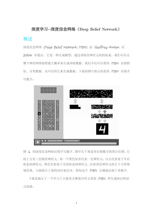
深度学习--深度信念网络(Deep Belief Network)概述深度信念网络(Deep Belief Network, DBN) 由Geoffrey Hinton 在2006 年提出。
它是一种生成模型,通过训练其神经元间的权重,我们可以让整个神经网络按照最大概率来生成训练数据。
我们不仅可以使用DBN 识别特征、分类数据,还可以用它来生成数据。
下面的图片展示的是用DBN 识别手写数字:图 1 用深度信念网络识别手写数字。
图中右下角是待识别数字的黑白位图,它的上方有三层隐性神经元。
每一个黑色矩形代表一层神经元,白点代表处于开启状态的神经元,黑色代表处于关闭状态的神经元。
注意顶层神经元的左下方即使别结果,与画面左上角的对应表比对,得知这个DBN 正确地识别了该数字。
下面是展示了一个学习了大量英文维基百科文章的DBN 所生成的自然语言段落:In 1974 Northern Denver had been overshadowed by CNL, and several Irish intelligence agencies in the Mediterranean region. However, on the Victoria, Kings Hebrew stated that Charles decided to escape during analliance. The mansion house was completed in 1882, the second in its bridge are omitted, while closing is the proton reticulum composed below it aims, such that it is the blurring of appearing on any well-paid type of box printer.DBN 由多层神经元构成,这些神经元又分为显性神经元和隐性神经元(以下简称显元和隐元)。

A Fast Learning Algorithm for Deep Belief Nets (2006)- 首次提出layerwise greedy pretraining的方法,开创deep learning方向。
layerwise pretraining的Restricted Boltzmann Machine (RBM)堆叠起来构成Deep Belief Network (DBN),其中训练最高层的RBM时加入了label。
之后对整个DBN进行fine-tuning。
在MNIST 数据集上测试没有严重过拟合,得到了比Neural Network (NN)更低的test error。
Reducing the Dimensionality of Data with Neural Networks (2006)- 提出deep autoencoder,作为数据降维方法发在Science上。
Autoencoder是一类通过最小化函数集对训练集数据的重构误差,自适应地编解码训练数据的算法。
Deep autoencoder 模型用Contrastive Divergence (CD)算法逐层训练重构输入数据的RBM,堆叠在一起fine-tuning最小化重构误差。
作为非线性降维方法在图像和文本降维实验中明显优于传统方法。
Learning Deep Architectures for AI (2009)- Bengio关于deep learning的tutorial,从研究背景到RBM和CD再到数种deep learning算法都有详细介绍。
还有丰富的reference。
于是也有个缺点就是太长了。
A Practical Guide to Training Restricted Boltzmann Machines (2010)- 如果想要自己实现deep learning算法,这篇是不得不看的。
我曾经试过自己写但是效果很不好,后来看到它才知道算法实现中还有很多重要的细节。

《深度学习相关研究综述》篇一一、引言随着科技的飞速发展,深度学习作为人工智能领域的重要分支,已经成为当前研究的热点。
深度学习以其强大的特征学习和表示学习能力,在图像识别、语音识别、自然语言处理、机器翻译等多个领域取得了显著的成果。
本文旨在全面综述深度学习的基本原理、发展历程、主要应用以及当前面临的挑战与未来发展趋势。
二、深度学习的基本原理与发展深度学习是基于神经网络的一种机器学习方法,其核心思想是通过构建多层神经网络来模拟人脑的思维方式,实现从原始数据中自动提取高级特征和抽象表示的目的。
深度学习的理论基础主要来源于人工神经网络、统计学和优化理论等学科。
随着硬件技术的进步和计算能力的提升,深度学习的发展经历了从浅层学习到深层学习的过程。
早期的神经网络模型由于计算资源的限制,通常只有几层结构,难以处理复杂的任务。
而随着深度学习算法的改进和计算机性能的飞跃,深度神经网络的层数不断增加,能够更好地处理大规模数据和复杂任务。
三、深度学习的主要应用1. 图像识别:深度学习在图像识别领域取得了显著的成果,如人脸识别、物体检测、图像分类等。
通过训练深度神经网络,可以自动提取图像中的特征,实现高精度的识别效果。
2. 语音识别:深度学习在语音识别领域也取得了重要突破,如语音合成、语音转文字等。
通过构建大规模的语音数据集和复杂的神经网络模型,可以实现高度逼真的语音合成和高效的语音转文字功能。
3. 自然语言处理:深度学习在自然语言处理领域也有广泛的应用,如机器翻译、情感分析、问答系统等。
通过构建语言模型和上下文感知模型,可以有效地理解和生成自然语言文本。
4. 机器翻译:深度学习在机器翻译领域的应用已经取得了巨大的成功。
通过训练大规模的平行语料库和复杂的神经网络模型,可以实现高质量的翻译效果。
四、当前面临的挑战与未来发展趋势尽管深度学习在多个领域取得了显著的成果,但仍面临一些挑战和问题。
首先,深度学习的可解释性仍然是一个亟待解决的问题。

《深度学习在计算机视觉领域的若干关键技术研究》篇一一、引言随着科技的飞速发展,深度学习在计算机视觉领域的应用越来越广泛。
计算机视觉,作为人工智能的重要分支,已经深入到我们生活的方方面面,如人脸识别、自动驾驶、医疗影像分析等。
本文将就深度学习在计算机视觉领域的若干关键技术进行深入探讨。
二、深度学习基础深度学习是机器学习的一个分支,其核心在于神经网络。
神经网络通过模拟人脑神经元的结构和工作方式,可以学习和理解复杂的模式。
在计算机视觉领域,深度学习主要通过卷积神经网络(CNN)实现图像的识别和分类。
三、关键技术研究1. 卷积神经网络(CNN)卷积神经网络是深度学习在计算机视觉领域的重要应用。
它通过卷积操作提取图像的局部特征,然后通过全连接层进行分类或回归。
CNN在图像分类、目标检测、语义分割等领域有着广泛的应用。
近年来,随着深度学习的不断发展,CNN的模型结构也在不断优化,如残差网络(ResNet)、轻量级网络(MobileNet)等。
2. 生成对抗网络(GAN)生成对抗网络是一种无监督学习的深度学习模型,由生成器和判别器组成。
GAN在计算机视觉领域的应用主要包括图像生成、图像修复、超分辨率等。
通过生成器和判别器的对抗训练,GAN 可以生成高质量的图像,为计算机视觉领域带来了新的可能性。
3. 迁移学习与微调迁移学习是利用在大数据集上预训练的模型来辅助小样本数据的训练。
在计算机视觉领域,可以利用在大规模图像数据集上预训练的模型(如ResNet),然后通过微调(fine-tuning)来适应特定的任务。
迁移学习和微调可以有效提高模型的性能,同时降低模型的训练成本。
四、应用领域分析1. 人脸识别深度学习在人脸识别领域的应用已经非常成熟。
通过卷积神经网络提取人脸特征,然后利用分类器进行人脸识别。
人脸识别技术在安防、金融、支付等领域有着广泛的应用。
2. 自动驾驶自动驾驶是计算机视觉的另一重要应用领域。
通过深度学习算法分析道路情况、行人、车辆等信息,然后对汽车进行决策和控制。
深度学习领域的最新研究成果随着人工智能技术的不断发展,深度学习在当前的科技领域中受到了广泛的关注和重视。
随着深度学习领域的不断发展,各种各样新的研究成果也不断涌现,下面将对深度学习领域的最新研究成果进行一一阐述。
一、深度神经网络优化技术深度学习模型在处理大规模数据时面临的一个主要问题便是优化问题。
近年来,学者们通过对深度神经网络不断的优化,使得深度学习模型取得了显著的进步。
其中,一些优化算法如AdaGrad、RMSProp、Adam、Nadam等不断被提出并得到了广泛应用。
此外,还有一些具有更强优化能力的策略如Orthogonal正交初始化、Dropout、Batch Normalization等被广泛应用。
二、深度学习在自然语言处理中的应用自然语言处理是人工智能领域中的重要方向之一。
随着深度学习技术的发展,深度学习在自然语言处理中的应用也取得了重要的进展,其中一些最新的研究进展主要包括以下几个方面:1. 语言模型语言模型是自然语言处理的基本问题之一。
近年来,基于深度学习技术的语言模型如RNN(循环神经网络)、LSTM(长短时记忆的循环神经网络)等不断涌现,并在许多自然语言处理的问题中取得了显著进展,例如文本分类、问答系统等。
2. 机器翻译机器翻译是一个颇为复杂的问题,其核心是将一种语言的文本自动转化为另一种语言的文本。
基于深度学习的机器翻译已经成为当今自然语言处理中的核心问题。
深度学习在机器翻译中的应用包括循环神经网络、卷积神经网络、Transformer等。
3. 文本摘要文本摘要是自然语言处理中重要的问题之一,其目标是自动地抽取并压缩输入的长文本内容,生成一个简洁的摘要。
在传统的文本摘要方法中,主要采用的是基于规则的方法或统计方法,而基于深度学习的自动化文本摘要方法受到了广泛关注。
深度学习在文本摘要中的应用包括循环神经网络、卷积神经网络等。
三、深度学习在图像处理中的应用在图像处理领域中,深度学习也已经成为了一种最常用的技术。
深度学习技术的最新研究动态在人工智能领域,深度学习无疑是近年来最受瞩目的明星。
随着计算能力的提升和大数据的积累,深度学习模型在图像识别、自然语言处理、医疗诊断等多个领域取得了显著的进展。
本文将探讨深度学习技术的一些最新研究动态,并分析其对相关领域的潜在影响。
语言模型的进化是深度学习领域的一个热点。
近年来,如BERT、GPT等模型通过大规模数据训练,展现了惊人的理解和生成能力。
基于这些模型,研究者正在探索更为复杂的多模态学习,尝试让机器不仅理解文本,还能处理图像、声音等多种信息。
例如,最新的研究试图将视觉信息与语言模型相结合,以实现更精确的图像标注或更生动的机器描述。
在强化学习领域,深度学习技术的结合使得智能体能够在复杂的环境下进行高效学习。
AlphaGo的成功仅仅是个开始,最新的研究正在将深度强化学习应用于自动驾驶、机器人操控等领域。
通过模拟人类大脑的奖励机制,智能体可以在不断的试错中学习到最优策略,这在提高自动化系统的适应性和鲁棒性方面显示出巨大潜力。
在神经网络结构方面,新型架构层出不穷。
为了解决深层网络训练困难的问题,一些研究提出了新的网络设计,如残差网络、稠密连接网络等。
这些结构通过改善梯度流动,使得上百层的网络训练成为可能。
此外,神经架构搜索这一领域也在快速发展,利用算法自动搜索最优的网络结构,极大地提高了模型设计的自动化水平。
深度学习在医疗领域的应用也日益广泛。
从疾病诊断到新药研发,深度学习技术正帮助科研人员突破传统方法的局限。
例如,通过深度学习分析医学影像,可以辅助医生更快地识别出肿瘤等病变;同时,利用深度学习对化合物数据库进行筛选,可以加速药物候选分子的发现过程。
深度学习技术的最新研究动态表明,无论是在模型架构、学习方法还是应用领域,该技术都在不断突破自我,展现出强大的生命力。
尽管存在诸如黑盒问题、数据依赖性强等挑战,但随着研究的深入,我们有理由相信深度学习将在不久的将来,为人类社会带来更多革命性的变革。
关于深度学习的作文英文回答:Deep learning is a subfield of machine learning that focuses on training artificial neural networks to learn and make predictions. It has gained significant attention and popularity in recent years due to its ability to handle complex and large-scale data sets. Deep learning models are capable of automatically extracting features from raw data, which eliminates the need for manual feature engineering. This makes deep learning particularly effective in tasks such as image and speech recognition, natural language processing, and recommendation systems.One of the key advantages of deep learning is itsability to learn from unstructured data. Traditional machine learning algorithms often require structured and pre-processed data, which can be time-consuming and labor-intensive. Deep learning algorithms, on the other hand, can directly process raw data, such as images, audio, and text,without the need for explicit feature extraction. This allows deep learning models to capture complex patterns and relationships that may not be apparent to human experts.Another strength of deep learning is its scalability. Deep neural networks can be trained on large-scale datasets with millions or even billions of examples. This enables deep learning models to learn from diverse and representative data, leading to improved generalization and performance. For example, in image recognition tasks, deep learning models have achieved state-of-the-art performance by training on massive image datasets such as ImageNet.Furthermore, deep learning models are highly flexible and can be adapted to various domains and applications. They can be trained to solve a wide range of problems, including object detection, speech synthesis, sentiment analysis, and drug discovery. The versatility of deep learning makes it a powerful tool for addressing complex real-world challenges.中文回答:深度学习是机器学习的一个子领域,专注于训练人工神经网络以学习和进行预测。
《深度学习相关研究综述》篇一一、引言深度学习作为人工智能领域的一个重要分支,近年来在学术界和工业界引起了广泛的关注。
它通过模拟人脑神经网络的运作方式,实现对复杂数据的处理和识别,从而在计算机视觉、自然语言处理、语音识别等多个领域取得了显著的成果。
本文将对深度学习的基本原理、发展历程、主要应用以及当前研究热点进行综述。
二、深度学习的基本原理与发展历程深度学习是机器学习的一个分支,其核心思想是通过构建多层神经网络来模拟人脑神经网络的运作方式。
它通过大量的训练数据,使模型学习到数据的内在规律和表示方法,从而实现更加精准的预测和分类。
自深度学习概念提出以来,其发展经历了几个重要阶段。
早期的神经网络由于计算能力的限制,模型深度较浅,无法充分挖掘数据的内在规律。
随着计算能力的不断提升,尤其是GPU等硬件设备的普及,深度学习的模型深度逐渐增加,取得了显著的成果。
同时,随着数据量的不断增长和大数据技术的不断发展,深度学习的应用领域也在不断扩大。
三、深度学习的主要应用1. 计算机视觉:深度学习在计算机视觉领域的应用非常广泛,包括图像分类、目标检测、人脸识别等。
通过深度神经网络,可以实现图像的自动识别和分类,从而在安防、医疗、自动驾驶等领域发挥重要作用。
2. 自然语言处理:深度学习在自然语言处理领域也取得了显著的成果,包括语音识别、文本分类、机器翻译等。
通过深度神经网络,可以实现对人类语言的自动理解和生成,从而在智能问答、智能助手等领域发挥重要作用。
3. 语音识别:深度学习在语音识别领域也具有广泛的应用,如语音合成、语音识别等。
通过训练深度神经网络模型,可以实现高质量的语音合成和准确的语音识别。
4. 其他领域:除了上述应用外,深度学习还在推荐系统、医疗影像分析、无人驾驶等领域发挥了重要作用。
四、当前研究热点1. 模型优化:针对深度学习模型的优化是当前研究的热点之一。
研究者们通过改进模型结构、优化算法等方式,提高模型的性能和计算效率。
Deeply-Supervised NetsChen-Yu Lee ∗Dept.of EECS,UCSD chl260@ Saining Xie ∗Dept.of CSE and CogSci,UCSDs9xie@Patrick Gallagher Dept.of CogSci,UCSD rexaran@ Zhengyou Zhang Microsoft Research zhang@ Zhuowen Tu †Dept.of CogSci,UCSD ztu@Abstract Our proposed deeply-supervised nets (DSN)method simultaneously minimizesclassification error while making the learning process of hidden layers direct and transparent.We make an attempt to boost the classification performance by study-ing a new formulation in deep networks.Three aspects in convolutional neural networks (CNN)style architectures are being looked at:(1)transparency of the intermediate layers to the overall classification;(2)discriminativeness and robust-ness of learned features,especially in the early layers;(3)effectiveness in training due to the presence of the exploding and vanishing gradients.We introduce “com-panion objective”to the individual hidden layers,in addition to the overall objec-tive at the output layer (a different strategy to layer-wise pre-training).We extend techniques from stochastic gradient methods to analyze our algorithm.The advan-tage of our method is evident and our experimental result on benchmark datasets shows significant performance gain over existing methods (e.g.all state-of-the-art results on MNIST,CIFAR-10,CIFAR-100,and SVHN).1IntroductionMuch attention has been given to a resurgence of neural networks,deep learning (DL)in particular,which can be of unsupervised [10],supervised [12],or a hybrid form [18].Significant performance gain has been observed,especially in the presence of large amount of training data,when deep learning techniques are used for image classification [11,16]and speech recognition [4].On the one hand,hierarchical and recursive networks [7,10,12]have demonstrated great promise in auto-matically learning thousands or even millions of features for pattern recognition;on the other hand concerns about deep learning have been raised and many fundamental questions remain open.Some potential problems with the current DL frameworks include:reduced transparency and dis-criminativeness of the features learned at hidden layers [31];training difficulty due to exploding and vanishing gradients [8,22];lack of a thorough mathematical understanding about the algorithmic behavior,despite of some attempts made on the theoretical side [6];dependence on the availability of large amount of training data [11];complexity of manual tuning during training [15].Neverthe-less,DL is capable of automatically learning and fusing rich hierarchical features in an integrated framework.Recent activities in open-sourcing and experience sharing [11,5,2]have also greatly helped the adopting and advancing of DL in the machine learning community and beyond.Several techniques,such as dropout [11],dropconnect [19],pre-training [4],and data augmentation [24],have been proposed to enhance the performance of DL from various angles,in addition to a vari-ety of engineering tricks used to fine-tune feature scale,step size,and convergence rate.Features ∗equal contribution†Corresponding author.Patent disclosure,UCSD Docket No.SD2014-313,filed on May 22,2014.a r X i v :1409.5185v 2 [s t a t .M L ] 25 S e p 2014(a)DSN illustration(b)functionsFigure1:Network architecture for the proposed deeply-supervised nets(DSN). learned automatically by the CNN algorithm[12]are intuitive[31].Some portion of features,es-pecially for those in the early layers,also demonstrate certain degree of opacity[31].Thisfinding is also consistent with an observation that different initializations of the feature learning at the early layers make negligible difference to thefinal classification[4].In addition,the presence of vanishing gradients also makes the DL training slow and ineffective[8].In this paper,we address the feature learning problem in DL by presenting a new algorithm,deeply-supervised nets(DSN),which en-forces direct and early supervision for both the hidden layers and the output layer.We introduce companion objective to the individual hidden layers,which is used as an additional constraint(or a new regularization)to the learning process.Our new formulation significantly enhances the per-formance of existing supervised DL methods.We also make an attempt to provide justification for our formulation using stochastic gradient techniques.We show an improvement of the convergence rate of the proposed method over standard ones,assuming local strong convexity of the optimization function(a very loose assumption but pointing to a promising direction).Several existing approaches are particularly worth mentioning and comparing with.In[1],layer-wise supervised pre-training is performed.Our proposed method does not perform pre-training and it emphasizes the importance of minimizing the output classification error while reducing the prediction error of each individual layer.This is important as the backpropagation is performed altogether in an integrated framework.In[26],label information is used for unsupervised learning. Semi-supervised learning is carried in deep learning[30].In[28],an SVM classifier is used for the output layer,instead of the standard softmax function in the CNN[12].Our framework(DSN),with the choice of using SVM,softmax or other classifiers,emphasizes the direct supervision of each intermediate layer.In the experiments,we show consistent improvement of DSN-SVM and DSN-Softmax over CNN-SVM and CNN-Softmax respectively.We observe all state-of-the-art results on MNIST,CIFAR-10,CIFAR-100,and SVHN.It is also worth mentioning that our formulation is inclusive to various techniques proposed recently such as averaging[24],dropconnect[19],and Maxout[9].We expect to see more classification error reduction with careful engineering for DSN.2Deeply-Supervised NetsIn this section,we give the main formulation of the proposed deeply-supervised nets(DSN).We focus on building our infrastructure around supervised CNN style frameworks[12,5,2]by intro-ducing classifier,e.g.SVM model[29],to each layer.An early attempt to combine SVM with DL was made in[28],which however has a different motivation with ours and only studies the output layer with some preliminary experimental results.2.1MotivationWe are motivated by the following simple observation:in general,a discriminative classifier trainedon highly discriminative features will display better performance than a discriminative classifiertrained on less discriminative features.If the features in question are the hidden layer feature maps of a deep network,this observation means that the performance of a discriminative classifier trained using these hidden layer feature maps can serve as a proxy for the quality/discriminativeness of those hidden layer feature maps,and further to the quality of the upper layer feature maps.By making appropriate use of this feature quality feedback at each hidden layer of the network,we are able to directly influence the hidden layer weight/filter update process to favor highly discriminative feature maps.This is a source of supervision that acts deep within the network at each layer;when our proxy for feature quality is good,we expect to much more rapidly approach the region of good features than would be the case if we had to rely on the gradual backpropagation from the output layer alone.We also expect to alleviate the common problem of having gradients that“explode”or “vanish”.One concern with a direct pursuit of feature discriminativeness at all hidden layers is that this might interfere with the overall network performance,since it is ultimately the feature maps at the output layer which are used for thefinal classification;our experimental results indicate that this is not the case.Our basic network architecture will be similar to the standard one used in the CNN framework.Our additional deep feedback is brought in by associating a companion local output with each hidden layer.We may think of this companion local output as analogous to thefinal output that a truncated network would have produced.Backpropagation of error now proceeds as usual,with the crucial difference that we now backpropagate not only from thefinal layer but also simultaneously from our local companion output.The empirical result suggests the following main properties of the companion objective:(1)it acts as a kind of feature regularization(although an unusual one),which leads to significant reduction to the testing error but not necessarily to the train error;(2)it results in faster convergence,especially in presence of small training data(see Figure(2)for an illustration on a running example).2.2FormulationWe focus on the supervised learning case and let S={(X i,y i),i=1..N}be our set of input training data where sample X i∈R n denotes the raw input data and y i∈{1,..,K}is the corre-sponding groundtruth label for sample X i.We drop i for notational simplicity,since each sample is considered independently.The goal of deep nets,specifically convolutional neural networks(CNN) [12],is to learn layers offilters and weights for the minimization of classification error at the output layer.Here,we absorb the bias term into the weight parameters and do not differentiate weights fromfilters and denote a recursive function for each layer m=1..M as:Z(m)=f(Q(m)),and Z(0)≡X,(1)Q(m)=W(m)∗Z(m−1).(2) M denotes the total number of layers;W(m),m=1..M are thefilters/weights to be learned;Z(m−1) is the feature map produced at layer m−1;Q(m)refers to the convolved/filtered responses on the previous feature map;f()is a pooling function on Q;Combining all layers of weights givesW=(W(1),...,W(M)).Now we introduce a set of classifiers,e.g.SVM(other classifiers like Softmax can be applied and we will show results using both SVM and Softmax in the experiments),one for each hidden layer,w=(w(1),...,w(M−1)),in addition to the W in the standard CNN framework.We denote the w(out)as the SVM weights for the output layer.Thus,we build our overall combined objective function as:w(out) 2+L(W,w(out))+M−1m=1αm[ w(m) 2+ (W,w(m))−γ]+,(3)whereL(W,w(out))=y k=y[1−<w(out),φ(Z(M),y)−φ(Z(M),y k)>]2+(4)and(W,w(m))=y k=y[1−<w(m),φ(Z(m),y)−φ(Z(m),y k)>]2+(5)We name L(W,w(M))as the overall loss(output layer)and (W,w(m))as the companion loss (hidden layers),which are both squared hinge losses of the prediction errors.The above formulation can be understood intuitively:in addition to learning convolution kernels and weights,W ,as in the standard CNN model[12],enforcing a constraint at each hidden layer for directly making a good label prediction gives a strong push for having discriminative and sensible features at each individual layer.In eqn.(3), w(out) 2and L(W,w(out))are respectively the margin and squared hinge loss of the SVM classifier(L2SVM1)at the output layer(we omit the balance term C in front of the hinge for notational simplicity);in eqn.(4), w(m) 2and (W,w(m))are respectively the margin and squared hinge loss of the SVM classifier at each hidden layer.Note that for each (W,w(m)),the w(m)directly depends on Z(m),which is dependent on W1,..,W m up to the m th layer.L(W,w(out))depends on w(out),which is decided by the entire W.The second term in eqn.(3)often goes to zero during the course of training;this way,the overall goal of producing good classification of the output layer is not altered and the companion objective just acts as a proxy or regularization.This is achieved by havingγas a threshold(a hyper parameter)in the second term of eqn.(3)with a hinge loss:once the overall value of the hidden layer reaches or is belowγ,it vanishes and no longer plays role in the learning process.αm balances the importance of the error in the output objective and the companion objective.In addition,we could use a simple decay function asαm×0.1×(1−t/N)→αm to enforce the second term to vanish after certain number of iterations,where t is the epoch step and N is the total number of epochs(wheather or not to have the decay onαm might vary in different experiments although the differences may not be very big). To summarize,we describe this optimization problem as follows:we want to learnfilters/weights W for the entire network such that an SVM classifier w(out)trained on the output feature maps (that depend on thosefilters/features)will display good performance.We seek this output perfor-mance while also requiring some“satisfactory”level of performance on the part of the hidden layer classifiers.We are saying:restrict attention to the parts of feature space that,when considered at the internal layers,lead to highly discriminative hidden layer feature maps(as measured via our proxy of hidden-layer classifier performance).The main difference between eqn.(3)and previous attempts in layer-wise supervised training is that we perform the optimization altogether with a ro-bust measure(or regularization)of the hidden layer.For example,greedy layer-wise pretraining was performed as either initialization orfine-tuning which results in some overfitting[1].The state-of-the-art benchmark results demonstrate the particular advantage of our formulation.As shown in Figure2(c),indeed both CNN and DSN reach training error near zero but DSN demonstrates a clear advantage of having a better generalization capability.To train the DSN model using SGD,the gradients of the objective function w.r.t the parameters in the model are:∂F∂w(out)=2w(out)−2y k=y[φ(Z(M),y)−φ(Z(M),y k)][1−<w(out),φ(Z(M),y)−φ(Z(M),y k)>]+∂F∂w(m)=αm2w(m)−2y k=y[φ(Z(m),y)−φ(Z(m),y k)][1−<w(m),φ(Z(m),y)−φ(Z(m),y k)>]+,otherwise 0,if w(m) 2+ (W,w(m))≤γ(6)The gradient w.r.t W just follows the conventional CNN based model plus the gradient that directly comes from the hidden layer supervision.Next,we provide more discussions to and try to understand intuitively about our formulation,eqn.(3).For ease of reference,we write this objective function asF(W)≡P(W)+Q(W),(7)where P(W)≡ w(out) 2+L(W,w(out))and Q(W)≡ M−1m=1αm[ w(m) 2+ (W,w(m))−γ]+.2.3Stochastic Gradient Descent ViewWe focus on the convergence advantage of DSN,instead of the regularization to the generalization aspect.In addition to the present problem in CNN where learned features are not always intuitive and discriminative[31],the difficulty of training deep neural networks has been discussed[8,22].1It makes negligible difference between L1SVM and L2SVM.As we can observe from eqn.(1)and(2),the change of the bottom layer weights get propagated through layers of functions,leading to exploding or vanishing gradients[22].Various techniques and parameter tuning tricks have been proposed to better train deep neural networks,such as pre-training and dropout[11].Here we provide a somewhat loose analysis to our proposed formulation, in a hope to understand its advantage in effectiveness.The objective function in deep neural networks is highly non-convex.Here we make the follow-ing assumptions/observations:(1)the objective/energy function of DL observes a large“flat”area around the“optimal”solution where any result has a similar performance;locally we still assume a convex(or evenλ-strongly convex)function whose optimization is often performed with stochastic gradient descent algorithm[3].The definition ofλ-strongly convex is standard:A function F(W)isλ-strongly convex if ∀,W,W ∈W and any subgradient g at W,F(W )≥F(W)+<g,W −W>+λ2W −W 2,(8)and the update rule in Stochastic Gradient Descent(SGD)at step t is W t+1=ΠW(W t−ηtˆg), whereηt=Θ(1/t)refers to the step rate andΠW helps to project onto the space of W.Let W∗be the optimum solution,upper bounds for E[ W T−W∗ 2]and E[(F(W T)−F(W∗)2]in[23] for the strongly convex function,and E[(F(W T)−F(W∗)2]for convex function in[25].Here we make an attempt to understand the convergence of eqn.(8)w.r.t.E[ W T−W∗ 2],due to the presence of large area offlat function shown in Figure(1.b).In[21],a convergence rate is given for the M-estimators with locally convex function with compositional loss and regularization terms. Both terms in eqn.(8)here refer to the same class label prediction error,a reason for calling the second term as companion objective.Our motivation is two-fold:(1)encourage the features learned at each layer to be directly discriminative for class label prediction,while keeping the ultimate goal of minimizing class label prediction at the output layer;(2)alleviate the exploding and vanishing gradients problem as each layer now has a direct supervision from the ground truth labels.One might raise a concern that learning highly discriminative intermediate stagefilters may not necessarily lead to the best prediction at the output layer.An illustration can been seen in Figure(1.b).Next, we give a loose theoretical analysis to our framework,which is also validated by comprehensive experimental studies with overwhelming advantages over the existing methods.Definition We name Sγ(F)={W:F(W)≤γ}as theγ-feasible set for a function F(W)≡P(W)+Q(W).First we show that a feasible solution for Q(W)leads to a feasible one to P(W).That is:Lemma1∀m,m =1..M−1,and m >m if w(m) 2+ ((ˆW(1),..,ˆW(m)),w(m))≤γthen there exists(ˆW(1),..,ˆW(m),..,ˆW(m ))such that w(m ) 2+ ((ˆW(1),..,ˆW(m)..,ˆW(m )),w(m ))≤γ.2Proof As we can see from an illustration of our network architecture shown infig.(1.a),for ∀(ˆW(1),..,ˆW(m))such that ((ˆW(1),..,ˆW(m)),w(m))≤γ.Then there is a trivial solution for the network for every layer j>m up to m ,we letˆW(j)=I and w(j)=w(m),meaning that the filters will be identity matrices.This results in ((ˆW(1),..,ˆW(m)..,ˆW(m )),w(m ))≤γ. Remark Lemma1shows that a good solution for Q(W)is also a good one for P(W),but it may not be the case the other way around.That is:a W that makes P(W)small may not necessarily produce discriminative features for the hidden layers to have a small Q(W).However,Q(W)can be viewed as a regularization term.Since P(W)observes a veryflat area near even zero on the training data and it is ultimately the test error that we really care about,we thus only focus on the W,W ,which makes both Q(W)and P(W)small.Therefore,it is not unreasonable to assume that F(W)≡P(W)+Q(W)and P(W)share the same optimal W .Let P(W))and P(W))be strongly convex around W , W −W 2≤D and W−W 2≤D, with P(W )≥P(W)+<gp,W −W>+λ12W −W 2and Q(W )≥Q(W)+<gq,W −W> 2Note that we drop the W(j),j>m since thefilters above layer m do not participate in the computation for the objective function of this layer.+λ12 W −W 2,where gp and gq are the subgradients for P and Q at W respectively.It can be directly seen that F (W )is also strongly convex and for subgradient gf of F (W )at W ,gf =gp +gq .Lemma 2Suppose E [ ˆgpt 2]≤G 2and E [ ˆgq t 2]≤G 2,and we use the update rule of W t +1=ΠW (W t −ηt (ˆgpt +ˆgq t ))where E [ˆgp t ]=gp t and E [ˆgq t ]=gq t .If we use ηt =1/(λ1+λ2)t ,then at time stamp TE [ W T −W 2]≤12G 2(λ1+λ2)2T(9)Proof Since F (W )=P (W )+Q (W ),it can be directly seen thatF (W )≥F (W )+<gp +gq ,W −W >+λ1+λ22 W −W 2.Based on lemma 1in [23],this upper bound directly holds. Lemma 3Following the assumptions in lemma 2,but now we assume ηt =1/t since λ1and λ2are not always readily available,then started from W 1−W 2≤D the convergence rate is bounded byE [ W T −W 2]≤e −2λ(ln T +0.578)D +(T −1)e −2λln(T −1)G 2(10)Proof Let λ=λ1+λ2,we haveF (W )−F (W t )≥<gf t ,W −W t >+λ2W −W t 2,and F (W )−F (W t )≥λ2 W t −W 2.Thus,<gf t ,W t −W >≥λ W t −W 2Therefore,with ηt =1/t ,E [ W t +1−W 2]=E [ ΠW (W t −ηt ˆgf t)−W 2]≤E [ W t −ηt ˆgf t−W 2]=E [ W t −W 2]−2ηt E [<gf t ,W t −W >]+ηt E [ ˆgf t2]≤(1−2λ/t )E [ W t −W 2]+G 2/t 2(11)With 2λ/t being small,we have 1−2λ/t ≈e −2λ/t .E [ W T −W 2]≤e −2λ(11+12+,..,1T )D +T −1t =1G 2t 2e −2λ(1t +1t +1+,..,1T −1)=e −2λ(ln T +0.578)D +G 2T −1t =1e −2ln(t )−2λ(ln(T −1)−2λln(t )≤e −2λ(ln T +0.578)D +(T −1)e −2λln(T −1)G 2Theorem 1Let P (W )be λ1-strongly convex and Q (W )be λ2-strongly convex near optimal Wand denote W (F )T and W (P )T as the solution after T iterations when applying SGD on F (W )andP (W )respectively.Then our deeply supervised framework in eqn.(3)improves the the speed over using top layer only by E [ W (P )T −W 2]E [ W (F )T −W 2]=Θ(1+λ22λ21),when ηt =1/λt,and,E [ W (P )T −W 2]E [ W (F )T −W 2]=Θ(e ln(T )λ2),when ηt =1/t.Proof Lemma 1shows the compatibility of the companion objective of Q w.r.t the output objective P .The first equation can be directly derived from lemma 2and the second equation can be seen from lemma 3.In general λ2 λ1which leads to a great improvement in convergence speed and the constraints in each hidden layer also helps to learning filters which are directly discriminative.3ExperimentsWe evaluate the proposed DSN method on four standard benchmark datasets:MNIST,CIFAR-10,CIFAR-100and SVHN.We follow a common training protocol used by Krizhevsky et al.[15]in all experiments.We use SGD solver with mini-batch size of 128at a fixed constant momentum value of 0.9.Initial value for learning rate and weight decay factor is determined based on the validation set.For a fair comparison and clear illustration of the effectiveness of DSN,we match the complexity of our model with that in network architectures used in [20]and [9]to have a comparable number of parameters.We also incorporate two dropout layers with dropout rate at panion objective at the convolutional layers is imposed to backpropagate the classification error guidance to the underlying convolutional layers.Learning rates are annealed during training by a factor of 20according to an epoch schedule determined on the validation set.The proposed DSN framework is not difficult to train and there are no particular engineering tricks adopted.Our system is built on top of widely used Caffe infrastructure [14].For the network architecture setup,we adopted the mlpconv layer and global averaged pooling scheme introduced in [20].DSN can be equipped with different types of loss functions,such as Softmax and SVM.We show performance boost of DSN-SVM and DSN-Softmax over CNN-SVM and CNN-Softmax respectively (see Figure (2.a)).The performance gain is more evident in presence of small training data (see Figure (2.b));this might partially ease the burden of requiring large training data for DL.Overall,we observe state-of-the-art classification error in all four datasets (without data augmentation),0.39%for MINIST,9.78%for CIFAR-10,34.57%for CIFAR-100,and 1.92%for SVHN (8.22%for CIFAR-10with data augmentation).All results are achieved without using averaging [24],which is not exclusive to our method.Figure (3)gives an illustration of some learned features.3.1MNISTepoch e r r o r number of training samples (k)e r r o r (%)epoche r r o r(a)(b)(c)Figure 2:Classification error on MNIST test.(a)shows test error of competing methods;(b)shows test error w.r.t.the training sample size.(c)training and testing error comparison.We first validate the effectiveness of the proposed DSN on the MNIST handwritten digits classifi-cation task [17],a widely and extensively adopted benchmark in machine learning.MNIST dataset consists of images of 10different classes (0to 9)of size 28×28with 60,000training samples and 10,000test samples.Figure 2(a)and (b)show results from four methods,namely:(1)conventional CNN with softmax loss (CNN-Softmax),(2)the proposed DSN with softmax loss (DSN-Softmax),(3)CNN with max-margin objective (CNN-SVM),and (4)the proposed DSN with max-margin objective (DSN-SVM).DSN-Softmax and DSN-SVM outperform both their competing CNN algo-rithms (DSN-SVM shows classification error of 0.39%under a single model without data whitening and augmentation).Figure 2(b)shows classification error of the competing methods when trained w.r.t.varying sizes of training samples (26%gain of DSN-SVM over CNN-Softmax at 500samples.Figure 2(c)shows a comparison of generalization error between CNN and DSN.3.2CIFAR-10and CIFAR-100CIFAR-10dataset consists of 32×32color images.A total number of 60,000images are split into 50,000training and 10,000testing images.The dataset is preprocessed by global contrast normal-ization.To compare our results with the previous state-of-the-art,in this case,we also augmented the dataset by zero padding 4pixels on each side,then do corner cropping and random flipping on the fly during training.No model averaging is done at the test phase and we only crop the center ofTable 1:MNIST classification result (without using data augmentation).Method Error(%)CNN [13]0.53Stochastic Pooling [32]0.47Network in Network [20]0.47Maxout Networks[9]0.45DSN (ours)0.39(a)by DSN (b)by CNNFigure 3:Visualization of the feature maps learned in the convolutional layer.a test sample.Table (2)shows our result.Our DSN model achieved an error rates of 9.78%without data augmentation and 8.22%with data agumentation (the best known result to our knowledge).DSN also provides added robustness to hyperparameter choice,in that the early layers are guided with direct classification loss,leading to a faster convergence rate and relieved burden on heavy hyperparameter tuning.We also compared the gradients in DSN and those in CNN,observing 4.55times greater gradient variance of DSN over CNN in the first convolutional layer.This is consistent with an observation in [9],and the assumptions and motivations we make in this work.To see what the features have been learned in DSN N,we select one example image from each of the ten categories of CIFAR-10dataset,run one forward pass,and show the feature maps learned from the first (bottom)convolutional layer in Figure (3).Only the top 30%activations are shown in each of the feature maps.Feature maps learned by DSN show to be more intuitive than those by CNN.CIFAR-10classification errorCIFAR-100classification errorMethod Error(%)No Data Augmentation Stochastic Pooling [32]15.13Maxout Networks [9]11.68Network in Network [20]10.41DSN (ours)9.78With Data Augmentation Maxout Networks [9]9.38DropConnect [19]9.32Network in Network [20]8.81DSN (ours)8.22Method Error(%)Stochastic Pooling [32]42.51Maxout Networks [9]38.57Tree based Priors [27]36.85Network in Network [20]35.68DSN (ours)34.57Table 2:Method comparison on CIFAR-10and CIFAR-100test data.CIFAR-100dataset is similar to CIFAR-10dataset,except that it has 100classes.The number of images for each class is then 500instead of 5,000as in CIFAR-10,which makes the classification task more challenging.We use the same network settings as in CIFAR-10.Table (2)shows previous best results and 34.57%is reported by DSN.The performance boost consistently shown on both CIFAR-10and CIFAR-100again demonstrates the advantage of the DSN method.Method Error(%)Stochastic Pooling[32] 2.80Maxout Networks[9] 2.47Network in Network[20] 2.35Dropconnect[19] 1.94DSN(ours) 1.92Table3:SVHN classification error.3.3Street View House NumbersStreet View House Numbers(SVHN)dataset consists of73,257digits for training,26,032digits for testing,and53,1131extra training samples on32×32color images.We followed the previous works for data preparation,namely:we select400samples per class from the training set and200 samples per class from the extra set.The remaining598,388images are used for training.We followed[9]to preprocess the dataset by Local Contrast Normalization(LCN).We do not do data augmentation in training and use only a single model in testing.Table3shows recent comparable results.Note that Dropconnect[19]uses data augmentation and multiple model voting.4ConclusionsIn this paper,we have presented a new formulation,deeply-supervised nets(DSN),attempting to make a more transparent learning process for deep learning.Evident performance enhancement over existing approaches has been obtained.A stochastic gradient view also sheds light to the understanding of our formulation.5AcknowledgmentsThis work is supported by NSF award IIS-1216528(IIS-1360566)and NSF award IIS-0844566 (IIS-1360568).We thank Min Lin,Naiyan Wang,Baoyuan Wang,Jingdong Wang,Liwei Wang, and David Wipf for help discussions.We are greatful for the generous donation of the GPUs by NVIDIA.References[1]Y.Bengio,mblin,D.Popovici,rochelle,U.D.Montral,and M.Qubec.Greedy layer-wisetraining of deep networks.In NIPS,2007.[2]J.Bergstra,O.Breuleux,F.Bastien,mblin,R.Pascanu,G.Desjardins,J.Turian,D.Warde-Farley,and Y.Bengio.Theano:a CPU and GPU math expression compiler.In Proceedings of the Python for Scientific Computing Conference(SciPy),June2010.[3]L.Bottou.Online algorithms and stochastic approximations.Cambridge University Press,1998.[4]G.E.Dahl,D.Yu,L.Deng,and A.Acero.Context-dependent pre-trained deep neural networks forlarge-vocabulary speech recognition.IEEE Tran.on Audio,Speech,and Lang.Proc.,20(1):30–42,2012.[5]J.Donahue,Y.Jia,O.Vinyals,J.Hoffman,N.Zhang,E.Tzeng,and T.Darrell.Decaf:A deep convolu-tional activation feature for generic visual recognition.In arXiv,2013.[6] D.Eigen,J.Rolfe,R.Fergus,and Y.LeCun.Understanding deep architectures using a recursive convo-lutional network.In arXiv:1312.1847v2,2014.[7]J.L.Elman.Distributed representations,simple recurrent networks,and grammatical.Machine Learning,7:195–225,1991.[8]X.Glorot and Y.Bengio.Understanding the difficulty of training deep feedforward neural networks.InAISTAT,2010.[9]I.J.Goodfellow,D.Warde-Farley,M.Mirza,A.C.Courville,and Y.Bengio.Maxout networks.In ICML,2013.[10]G.E.Hinton,S.Osindero,and Y.W.Teh.A fast learning algorithm for deep belief nets.Neural compu-tation,18:1527–1554,2006.[11]G.E.Hinton,N.Srivastava,A.Krizhevsky,I.Sutskever,and R.Salakhutdinov.Improving neural net-works by preventing co-adaptation of feature detectors.In CoRR,abs/1207.0580,2012.[12] F.J.Huang and rge-scale learning with svm and convolutional for generic object catego-rization.In CVPR,2006.[13]K.Jarrett,K.Kavukcuoglu,M.Ranzato,and Y.LeCun.What is the best multi-stage architecture forobject recognition?In ICCV,2009.。