FINITE ELEMENT SIMULATION OF RUBBERLIKE MATERIALS USED IN VIBRATION ISOLATORS

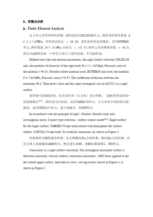
3、有限元分析3、Finite Element Analysis定义单元类型和材料参数，刚性面选用SOLID186单元，刚性体的弹性模量E = 2.1×105MPa，材料的泊松比γ =0.33；柔性体材料选用橡胶，采用HYPER86单元，弹性模量E = 7.84 MPa，泊松比γ = 0.47；材料之间的摩擦系数μ =0.3；然后在ANSYS里画一个和长方体尺寸相同的面，作为刚性面。

Defined unit type and material parameters, the rigid surface selection SOLID186 unit, the modulus of elasticity of the rigid body E = 2.1×105Mpa, Poisson's ratio of the material γ =0.33; Flexible rubber material used, HYPER86 unit used, the modulus E = 7.84 MPa, Poisson's ratioγ = 0.47; The coefficient of friction between the materialμ =0.3; Then draw a face and the same rectangular size in ANSYS as a rigid surface.按照刚-柔接触原则，仅对柔性体（长方体）划分网格。

接触类型选择面-面接触模式[6-8]，刚性面为目标面，选用TARGE170单元，长方体带半球的面为接触面，选用CONTA174单元，建立接触对。

如图3所示。

In accordance with the principle of rigid - flexible, flexible body only (rectangular) mesh. Contact type selection - surface contact mode[6-8], Rigid surface for the target surface, TARGE170 unit used,cuboid with hemisphere the contact surface, CONTA174 unit used, To establish contaction. As shown in Figure 3.约束条件为刚性面全约束，长方体横向面x方向约束，纵向面y方向约束。

Proceedings of the 5th Annual ISC Research SymposiumISCRS 2011April 7, 2011, Rolla, Missouri FINITE ELEMENT MODELING OF BIRD STRIKES AND PARAMETRICEV ALUATION USING DESIGN OF EXPERIMENTS (DOE)V. P. BheemreddyDepartment of Mechanical and Aerospace Engineering, Missouri S&Tvbqv8@Dr. K. ChandrashekharaDepartment of Mechanical and Aerospace Engineering, Missouri S&Tchandra@Dr. Thomas P. SchumanDepartment of Chemistry, Missouri S&Ttschuman@ABSTRACTOne of the major threats to Aviation industry is the in-flight impact of birds. Aircraft windshields are intensively vulnerable to damage and hence need a certification requirement for a proven level of impact resistance. Bird strike experiments are very expensive and henceforth explicit numerical modeling techniques have grown importance. This compilation mainly relies on the theory of hydrodynamic impact and addresses basic shockwave equations. A smooth particle hydrodynamics based approach is chosen and the numerical simulation is carried out using contact-impact coupling algorithm. The simulation is run using the nonlinear explicit finite element code LS-DYNA ver.971, developed by Lawrence Livermore National Laboratories. A traditional design of experiments approach, factorial design, has been utilized to facilitate the economical prediction of factors significantly affecting the pressure response in the bird strike analysis. Impact velocity, bird mass, bird aspect ratio, porosity and obliquity of impact are the various parameters investigated in the present work. The results show that main effects velocity and obliquity of impact, and ‘porosity x obliquity’ interaction effect, are the factors significantly affecting the pressure response in a bird strike analysis.1.INTRODUCTIONBird strikes have been a significant safety threat and unavoidable menaces to both civil and military aircrafts. The bird strike incident can have tragic consequences, especially for small generation aviation airplanes. Bird strikes cause significant economic loss to the aviation industry, estimated over $1.2 billion annually [1]. These incidents are critical during takeoff and landing phases. This is one reason for limiting the maximum airplane speeds to 250kt below 10000 ft altitudes [2].The forward-facing components of an aircraft such as windshields, leading edge structures, aircraft engines etc are often susceptible to such strikes. The U.S. Federal Aviation Administration (FAA) and European Joint Aviation Authority (JAA) have set certification standards which require an aircraft be designed to successfully complete a flight after an impact with a standard-size bird [2]. Further testing with higher impact velocities is carried out to determine the actual limits of the structure. The use of real birds lends realism to the test results but complicates the testing procedure, very costly and time consuming.The number of variables, the bird strike analysis deals with, is high. This makes the bird strike analysis complex. The various parameters include bird density, velocity and mass of bird, bird material configuration, high strain rates and contact properties. Most of the models, initially developed, used force-impulse equation. Semi-empirical equations were developed to simulate the entire impact event. However, in most of the cases, these models failed to predict the damage to its details. They failed to account for the complex interactions during the impact.Finite element analysis is capable of accurately simulating the bird impact, and thus the geometry of the impacted structure. The finite element method is good at simulating the transient loading of bird on the target. Because, the bird strike analysis deals with high strain rates, nonlinearity and large deformation accompany the impact. Finite element analysis is proved to deal with nonlinearities in structures and has the capability of predicting the penetration of bird following the initial hit.The nonlinear explicit finite element code LS-DYNA has been used by many researchers, especially in high velocity impacts. In the current investigation, LSTC LS-DYNA ver.971 will be used.The use of real birds has many drawbacks. One of the major drawbacks is the lack of repeatability. The impact loads vary from test to test. Testing with real birds also has sanitary and aesthetic disadvantages. Explicit numerical techniques have grown importance and are a viable alternative to several extensive and difficult experimental iterations of the test structure.A bird strike incident is characterized by high impact loads and short duration. The impact duration is typically in the range of milliseconds. An important step in the bird strike simulation is the development of an “artificial bird model.” The artificial bird models would replace real birds in actual impact tests. The accurate modeling of an artificial bird includes the shape and material modeling of the bird.Design of Experiments (DOE) is a systematic and rigorous methodology to solving engineering problems. DOE is the simultaneous study of several variables. Combining several variables in one study, the amount of simulation experimentation is dramatically reduced and yields greater knowledge. DOE is a viable tool for gaining knowledge through experimentation; increases possibility to extract large amount of information in a matrix, from a small fraction of data. A Design of Experiments (DOE) approach, factorial design, is used to statistically evaluate the significant factors and their interactions affecting the bird impact pressures.2.LITERATURE RIVIEWBird strike analysis is not a new problem and relatively good amount of work has been done. Barber et al. [3, 4] and Wilbeck et al. [5-7] conducted extensive experimentation on bird strike analysis and concluded the fluid like behavior of birds upon impact. Cassenti [8] developed the governing equations for the hugoniot pressure. Wilbeck [5] developed an empirical bird model based on the hydrodynamic theory and compared it with the experimental results. The empirical model was in good agreement with the experimental results for medium sized birds. Wilbeck also proposed equation of state [EOS] models for hugoniot shock phase and steady state phase. McCallum et al. [9] worked on using multi-material bird models. McCallum also worked on different bird geometries for the impact analysis. Huertas [10] and Goyal et al. [11] carried out a computational study on bird impact phenomenon using lagrangian, Arbitrary Lagrangian Eulerian (ALE) and Smooth Particle Hydrodynamics (SPH) formulations. Nizampatnam et al. [12, 13] worked extensively on multi-material heterogeneous bird models and equation of state [EOS] models, and made significant contribution.Not much work has been presented on investigating the behavior of various parameters of the bird. The study is limited and is done using the traditional one-factor-at-a-time (OFA T) experiments (i.e. simulation experiments). The one-factor-at-a-time (OFAT) experiments, however, can only estimate the individual behavior of factors; never the interaction. With the advancement of statistical Design of Experiments (DOE) approach, the interaction effects can also be explored. The present compilation uses factorial design of experiments methodology to conclude the terms significant to pressure response in a bird strike analysis.3.FINITE ELEMENT MODELING AND V ALIDATIONIn this section, a brief introduction to hydrodynamic theory is provided. The various phases in a bird strike analysis, Equation of State models are discussed. At the end, the finite element models considered for the bird strike analysis and the validation of simulation results with Wilbeck [5] analytical and experimental results are presented.3.1.Hydrodynamic TheoryThe theory of Hydrodynamics can be used to study high velocity impacts. The hydrodynamic theory is based on the belief that during impact the projectile material tends to behave as a fluid. The requirement for a material to flow is that the stresses generated during impact should exceed the strength of the material. The material strength and viscosity are neglected and a simple pressure-density-energy equation of state is used to describe the material behavior. In the Hydrodynamic approach, it is the material density which dominates the strength. This theory assumes that in a high velocity impact, the projectile material would behave as a fluid with same material density [5].3.2.Equation of State Models for BirdAn Equation of State (EOS) is a relation between state variables. It is a thermodynamic equation that describes the state of matter under a given set of physical conditions. It is a constitutive equation that provides mathematical relationship between two or more state functions such as temperature, volume, pressure and internal energy.P=P(V,E)=P(V,T) (1) where V, E and T are volume, internal energy and temperature respectively. Wilbeck [5] carried out extensive amount of research in finding out precise Equation of State models for the shock phase and steady state phase. The Equation of State model formulation for the Hugoniot phase is presented below.The shock wave progression and the condition ahead of and behind a shock moving through a material can be described by the following conservation laws:Conservation of massρ1u s=ρ2�u s−u p� (2) Conservation of momentumP1+ρ1u s2=P2+ρ2�u s−u p�2 (3) Conservation of EnergyP2u p=ρ1u s�E2−E1+u p22� (4) where u s is the shock velocity, u p is the translational particle velocity or simply projectile velocity, ρ1and ρ2are the respective densities of the material in front of the shock and behind it, E1 and E2 are the respective energies before and after compression, P1and P2are the pressures in unshocked and shocked regions respectively. Equations (2) and (3) can be combined to obtain Hugoniot pressure P H as below:P H=P2−P1=ρ1u s u p (5) From the above it is clear that the Hugoniot pressure is a function of initial projectile density, shock velocity and the projectile velocity. The shock velocity is unknown. For most solids and liquids, the shock velocity and particle velocity are related by the expression:u s=c0+ku p (6)where c 0 is isentropic wave speed and k is a constant. The above equation is called “linear Hugoniot.”If the bird is assumed to behave as a fluid and take the properties of water, the above relation takes the form:u s ,water =c 0,water +k water u p (7)where c 0,water is the velocity of sound in water, 1482.9 m/s and k water =2.0.From Equation (2) the continuity equation can be written as:u p s =1−ρ12=q (8) where the subscripts 1 and 2 refer to the regions in front of and behind it.Substituting Equation (8) into Equation (6) and re-arranging:u sc 0=11−kq(9) Substituting Equations (8) and (9) into Equation (5) gives:P H =ρ1c 02q()2(10) The pressure-density relationship for a one-dimensional shock developed by Cogolev takes the form:P H =A ��ρ21�B−1� (11)where A and B are material constants. Ruoff approximated the constants by the following expressions:A =ρ1c 02()(12) B =(4k −1) (13)where k is a constant.The Equation (11) can be re-arranged to obtain:ρ12=�P H+1�−1B� (14) All the real birds contain certain quantities of entrapped air. A homogeneous mixture of water and air was believed to behave as a real bird. When porosity effects are included, the linear Hugoniot no longer holds good for the relation becomes nonlinear. Wilbeck [5] used mixture theory to develop an Equation of State for the porous material.�ρ12�porous =(1−z )�ρ12�water +z �ρ12�air(15) where z is percentage by volume of air.The density ratio for water can be obtained from Equations (2) and (7). The Equations (8) and (10) can be used for air. So Equation (15) takes the form:�ρ1ρ2�porous =(1−z )�P H A+1�−1B�+z (1−q ) (16) Equation (16) has to be solved for the Hugoniot pressure generated during the impact.3.4. Finite Element ModelsIn this section, three different bird shapes are assumed, and validated with Wilbeck analytical model and experimental results [5]. The numerical simulation is carried out using the Smooth Particle Hydrodynamics (SPH).The smooth particle hydrodynamics was initially developed to investigate various astrophysical problems, and later extended to the field of computational fluid dynamics. This phenomenon is now being explored for its use in continuum mechanics. The main difference between the lagrangian and smooth particle hydrodynamics theories lies in the discretization of the continuum [14]. Smooth particle hydrodynamics is a meshless method. The lagrangian mesh is replaced with particles at the nodes. These particles are not directly connected to each other; the kernel function is the core of the method. Because the particles are not directly connected, this method suits well the bird impact phenomenon, large mesh distortions are not observed as opposed to the conventional lagrangian formulation. Throughout this compilation, the simulations are run using the smooth particle hydrodynamics in LS-DYNA.Figure 3 Simulation of cylindrical bird model at varioustime historiesFigure 4 Simulation of ‘cylinder with hemispherical ends’bird model at various time historiesFigure 5 Simulation of ellipsoidal bird model at varioustime historiesThree different bird geometries- cylindrical, cylinder with hemispherical ends, and ellipsoidal, are considered for the finite element bird validation. Majority of the birds responsible for damage in a bird strike are medium sized. And the maximum airplane speeds are limited to 250 kt below 10,000 ft altitudes [2]. The same velocity can be assumed for the bird. The SI unit equivalent is 128.6 m/s. Bird mass is fixed at 2 kg and an aspect ratio of 2 is assumed. The plate is considered to be rigid, to evaluate the bird model alone and neglecting the effect of target on the bird. Figures 3-5 show the simulation of finite element bird models at different time periods.The peak pressures, Hugoniot pressures, are extracted from the simulation results and plotted on a graph alongside Wilbeck analytical model and experimental results. Figure 6 shows the graph plotted with these results. Also simulations corresponding to the velocities 150 m/s, 200 m/s and 250 m/s, have been presented to validate the finite element model with the analytical model. It is clearly observed that the cylindrical model with hemispherical ends predicted the analytical model well. The cylindrical model with hemispherical ends under-estimated the result by only 7.73% (velocity at 250 kt [2] or 128.6 m/s). The cylindrical model had an error of 9.61% and the ellipsoidal model over-estimated the pressure by 25.97%. This large difference could be due to low contact area in case of ellipsoidal model.The artificial bird model predicted the pressure well; a parametric evaluation of this model using the Design of Experiments (DOE) approach can provide the relative significance of each of the parameters, which is very important.Figure 6 Comparison of Simulation Results with Wilbeck[5] Analytical Model and Experiments4. DESIGN OF EXPERIMENTSDesign of experiments is a discipline that has very broad application. It is a systematic and rigorous methodology to solving engineering problems; applies principles and techniques at data collection stage, ensuring the generation of valid, defensible and convincing inferences [15]. It is an efficient and cost-effective way to model and analyze the relationships that describe bird impact pressure variations.Typical one-factor-at-a-time (OFA T) experiments limit knowledge and can be a waste of time. In this context, the term experiments can be referred to simulation experiments. Design of Experiments (DOE) is the simultaneous study of several variables. Combining several variables in one study, the amount of simulation experimentation is dramatically reduced and yields greater knowledge. The major disadvantage of the one-factor-at-a-time strategy is that it fails to consider any possible interaction between the factors. Design of experiments is a viable tool for gaining knowledge through experimentation; increases possibility to extract large amount of information in a matrix, from a small fraction of data.Design of experiments approach has several advantages over traditional one-factor-at-a-time experimentation. Design of experiments requires far fewer tests for validating results, tending towards significant cost and time savings. It can detect the interactions between variables that cannot be revealed when varying one factor at a time. These interactions are significant and often prove to be the key to break through improvements.Many experiments involve the investigation of two or more factors. For these experiments, factorial designs are very efficient [15]. The most common case of these factorial designs involves ‘k’ factors each at two levels, generally referred to as ‘2k factorial designs’. These designs are widely used in ‘factor screening experiments’. Figure 7 contrasts a 23 factorial design with a one-factor-at-a-time experiment of equivalent replication [16].Figure 7 Comparison of two-level factorial designs (left)versus OFA T (right)The two-level factorial design with three factors requires eight runs in total, whereas a one-factor-at-a-time experiment for the same requires sixteen runs. Due to its efficient parallel processing, the factorial design trumps the serial one-factor-at-a-time methodology; the efficiency of the factorial design becomes more pronounced as the number of factors (k) increase.Designing a priori a numerical experiment is an important step in the factorial design- design of experiments approach.The experimental design mainly consists of selecting thefactors and their levels that will provide most of the information on the input-output relationship of a model in the presence of variation [16]. Five inputs (factors) have been considered responsible to pressures in a bird impact process. Different factorial level combinations are selected to ascertain the relative importance of each of these factors. The response variable of interest is the hugoniot pressure generated during the impact. Table 1 lists the factors and their levels under investigation, and the response variable of interest.The analysis is based on a 25 full-factorial experiment design. Running the full matrix of all possible factor combinations implies estimating all main and interaction effects [15]. The present design requires a total of 32 simulation experiments to be run. Table 2 lists the various input factor combinations and the corresponding pressure output.With a full-factorial experiment, a model containing five main effect terms, ten 2-factor interaction terms, ten 3-factor interaction terms, five 4-factor interaction terms, a 5-factor interaction term and a mean term, can be fitted. However, the present design has been limited to 2-factor interaction terms only. The higher order interaction terms have been omitted assuming that they are insignificant.A statistical hypothesis testing procedure called analysis of variance (ANOVA) is used to test the significance of the data. The analysis is carried out in SAS v9.2; the obtained analysis of variance results are shown in Table 3. The model accounts for most of the variability in the response, achieving an adjusted R2 of 0.8367. The R2 is found to be 0.9157; it measures the proportion of total variability explained by the model. However, the R2 statistic always increases as factors are added to the model, even if the factors are not significant. In view of this, the R2-adjusted is considered in majority of scenario. The adjusted R2 statistic is a statistic that is adjusted for the size of the model; it can actually decrease if non-significant terms are added to model [15].The p-value of 0.0058 corresponding to ‘porosity x obliquity’ interaction effect implies the conclusion that the interaction effect ‘porosity x obliquity’ has significant effect on the pressure response is made with 99.42% confidence. Or in simple lines, we say the porosity and obliquity interaction terms are significantly affecting the pressure response and need to be considered while modeling the phenomenon.Table 2 Design of experiment matrix listing the factorialThe similar conclusions are made on the main effects that are significantly affecting the pressure response. Because, the porosity and obliquity interaction terms are significant, we need not look into porosity and obliquity main effects. The main effects other than porosity and obliquity are looked into and the conclusion velocity main effect has significant influence on the pressure response is made with 99.99% confidence. The higher value of p can be explained in similar lines too. For example, the main effect, aspect ratio, has a p-value of 0.5161. This implies that the statement, aspect ratio has significant effect on the pressure response, is rejected with 48.39% confidence.5.CONCLUSIONSBird strikes are often unavoidable and can have tragic consequences to both civil and military aircrafts. The design of structural components against bird strikes requires indepth understanding of the bird strike phenomenon, which is quite complex inview of the convoluted and uneconomical experimental investigations. Explicit finite element analyses have grown importance and have become a viable alternative to development of artificial bird models. The finite element (FE) and design of experiments (DOE) methods are used in tandem to obtain a better understanding of the bird strike phenomenon. Finite element models with different geometries are compared to the experiment results and the empirical model developed by Wilbeck. Having validated the artificial bird model, factorial design of experiments approach is used, as opposed to one-factor-at-a-time (OFAT) experiments, to carry out parametric evaluation. The model signatures indicate that the velocity and obliquity main effects and ‘porosity x obliquity’ interaction effects are significant terms affecting the pressure response in a bird impact phenomenon. The present work can be furthered to bird strike on windshields with various material combinations and optimize the structural component design using response surface methodologies (RSM). 6.ACKNOWLEDGMENTSPartial support from Intelligent Systems Center is gratefully acknowledged.7.REFERENCES[1]Allan, J. R., 2006, “A Heuristic Risk AssessmentTechnique for Birdstrike Management at Airports,” RiskAnalysis, V olume 26, pp. 723-729.[2]Eschenfelder, P. F., 2005, “High Speed Flight at LowAltitude: Hazard to Commercial Aviation?” IBSC 27/WP I-3, International Bird Strike Committee.[3]Barber, J. P., Taylor, H. R., and Wilbeck, J. S., 1975,“Characterization of Bird Impacts on a Rigid Plate: Part 1,”Technical report AFFDL-TR-75-5.[4]Barber, J. P., Taylor, H. R., and Wilbeck, J. S., 1978,“Bird Impact Forces and Pressures on Rigid and CompliantTargets,” Technical report AFFDL-TR-77-60.[5]Wilbeck, J. S., 1977, “Impact Behavior of Low StrengthProjectiles,” PhD Dissertation, Texas A&M University. [6]Wilbeck, J. S., and Barber, J. P., 1978, “Bird ImpactLoading,” The Shock and Vibration Bulletin, V olume 48,pp. 115-122.[7]Wilbeck, J. S., and Rand, J. L., 1981, “The Development ofSubstitute Bird Model,” ASME Journal of Engineering forPower, V olume 103, pp. 725-730.[8]Cassenti, B. N., 1979, “Hugoniot Pressure Loading in SoftBody Impacts,” United Technologies Research Center, Connecticut.[9]McCallum, S. C., and Constantinou, C., 2005, “TheInfluence of Bird-Shape in Bird-Strike Analysis”, 5th European LSDYNA Users Conference.[10]Huertas, C. A., 2006, “Robust Bird-Strike Modeling usingLS-DYNA,” M.S. Thesis, University of Puerto Rico.[11]Goyal, V. K., Huertas, C. A., Borrero, J. R., and Leutwilers,T. R., 2006, “Robust Bird-Strike Modeling based on SPHFormulation using LS-DYNA,” AIAA 2006-1878, 47thAIAA/ASME/ASCE/AHS/ASC Structures, Structural Dynamics, and Materials Conference.[12]Nizampatnam, L. S., 2007, “Models and Methods for BirdStrike Load Predictions,” PhD Dissertation, Wichita StateUniversity.[13]Nizampatnam, L. S., and Horn, W. J., 2008, “Investigationof Equation of State Models for Predicting Bird Impact Loads,” AIAA-2008-682, 46th AIAA Aerospace SciencesMeeting and Exhibit.[14]Belytschko, T., Liu, W. K., and Moran, B., 2000,“Nonlinear Finite Elements of Continua and Structures,”Wiley Publications, First Edition.[15]Al-Momani, E., and Rawabdeh, I., 2008, “An Applicationof Finite Element Method and Design of Experiments inthe Optimization of Sheet Metal Blanking Process,” JordanJournal of Mechanical and Industrial Engineering, V olume2, pp. 53-63.[16]Montgomery, D. C., 2004, “Design and Analysis ofExperiments,” Wiley Publications, Sixth Edition.。

6采 掘本栏目编辑　李文民料为 42CrMo 钢，弹性模量为 212 GPa，泊松比为 0.28，密度为 7850 kg /m 3；硬质合金头材料为 YG 系列硬质合金，弹性模量为 600 GPa，泊松比为 0.22，密度为 14600 kg /m 3。

所研究的 3 种不同形状的截齿结构如图 1 所示。

(a) 截齿 A(b) 截齿 B(c) 截齿 C图 1 不同形状的截齿结构Fig 1 Structure of cutting picks with various shapes在 LS-DYNA 中对截齿进行建模。

采用 3D Solid 164 单元类型和柔性体材料模型 (MAT_PLASTIC_ KINEMATIC) 建立的截齿有限元模型如图 2 所示。

1.2 岩石本构模型在 LS-DYNA 中，利用接触碰撞中的分配参数法、岩石力学和显示动力学等理论，建立岩石截割工况模型。

选取岩石材料模型 13，含失效的弹塑性材料 (MAT_ISOTROPIC_ELASTIC_FAILURE)。

岩石基本参数为[9-10]：岩石密度为 2394 kg /m 3，硬度为 1176 MPa，塑性系数为 3.20，单轴抗压强度为 80 MPa，弹性模量为 8396.3 MPa，泊松比为 0.23。

由于岩石材料的物理机械性质参数在实际中难以获取，工程实践中常用坚固性系数 f 来综合反映岩石抵抗外力破碎能力，并以此推导出岩石的主要力学参数。

前苏联学者给出的坚固性系数 f 与岩石材料的最大抗压强度 f c 的关系为f c ＝10f 。

(1)当等效塑性应变达到失效应变，或当压应力达到失效压力时，材料就失效，即p n +1<p min 或 e e p ff >e m p ax ， (2)式中：p n +1 为 n +1 时刻的应变率参数；e e p ff 为等效塑性应变；p min 、e m p ax 分别为为用户定义的塑性失效应变和失效压力参数。

Simulation of dynamic compaction of loose granular soilsJ.L.Pan,A.R.SelbySchool of Engineering Science Laboratories,University of Durham,South Road,Durham DH13LE,UKReceived 15November 2000;accepted 1July 2002AbstractDynamic compaction is an efficient ground improvement technique for loose soils.The improvement is obtained by controlled high energy tamping and its effects vary with the soil properties and energy input.Various analytical methods have been used to simulate the effectiveness of dynamic compaction of loose soils,most of which were based on a rigid hammer striking a vertical soil column represented by springs,masses and dampers.This study simulated the dynamic compaction of loose soils under dynamic loads numerically,using ABAQUS q [Hibbit,Karlsson and Sorensen,Inc.,1998]to generate a full axisymmetric elasto-plastic finite element representation of the soils.The impact of the drop mass was modelled in two ways.Firstly,a force–time input derived from the characteristic shape of the deceleration of the mass was imposed.Secondly,a rigid body impacting collision onto the soil surface was parisons were made of the ground waves,peak particle accelerations with depth,mass penetration (crater depth)and peak particle velocity on ground surface.q 2002Civil-Comp Ltd and Elsevier Science Ltd.All rights reserved.Keywords:Dynamic compaction;Ground waves;Finite elements1.IntroductionDynamic compaction is a ground improvement tech-nique which is particularly effective for loose unsaturated granular soils.It has also been used successfully on cohesive soils of high void ratio,and on wastes and fills.A heavy weight (W )of 10–20Mg is dropped from a height (H )of some 10to 20m in a grid pattern across the treatment area.The objective is to densify the soils into a state of low void ratio,by compacting the soil fabric and expelling void fluids.Some ‘hammering’occurs local to the impact,which forms a dense plug of soils immediately below the drop mass.However,the main beneficial effect,to more considerable depths,is achieved from the outgoing high-energy ground waves,as shown in pression waves,or P-waves,are generated by the impact,which spread downwards and outwards on a spherical wave front.The energy density is maximum on the vertical axis of symmetry and reduces with increasing angle from the vertical axis.Also,as the wave penetrates to greater depth around a larger hemispherical front,the energy density attenuates (geometrically).Since the soil improvement is a function of particle vibration,the spread and attenuation of the P-waves define the zone of the soil which is compacted.Dynamic compaction has been studied experimentally by a number of researchers,notably West and Slocombe [2],Menard and Broise [3],Leonard et al.[4],Mayne et al.[5],Slocombe [6],Orje [7]and Kroge and Lindgren [8].These studies have shown the ranges of soils for which the method is most effective,and also that an empirical expression for depth of effective ground treatment is given by D ¼0:5p ðWH Þto 1.0p(WH ).Additionally,some studies showed the form of the deceleration–time curve of the drop mass,and some gave indications of surface vibrations.The technique has been studied analytically by Scott and Pearce [9],Mayne and Jones [10],Roesset et al.[11],Deeks and Randolph [12],and Thilakasiri et al.[13].Compu-tational models have been developed and calibrated effectively against site records by Chow et al.[14,15],based primarily on a one-dimensional wave equation.However,fully developed computational models of the wave patterns appear not to have been produced by computation.Modern computational packages are now available to model ground waves using finite/infinite elements to estimate outgoing compression,shear and surface waves,and to include elasto-plastic and compressible material behaviour.Site measurements of drop mass deceleration are becoming available,together with surface vibrations.0965-9978/02/$-see front matter q 2002Civil-Comp Ltd and Elsevier Science Ltd.All rights reserved.PII:S 0965-9978(02)00067-4Advances in Engineering Software 33(2002)631–640/locate/advengsoftGranular soil compaction in response to vibration is also better understood.The combination of these facilities offers the potential for progress in the understanding of ground waves and compaction.The objective of this study was to simulate numerically the ground waves generated during dynamic compaction of loose soils using ABAQUS q .The system was initially modelled in two different ways.Firstly,a force–time curve was applied,derived from the product of drop mass and deceleration–time,based on the typical damped half-sine wave form.The second,more ambitious,approach was to apply the impact of a rigid body to the soil parisons were made between the ground waves,peak particle accelerations with depth,mass penetration (crater depth)and peak particle velocity on ground surface generated during the dynamic compaction.The impact model was then used to study the effects due to changes in drop height,drop mass and soil properties,and for several drops.2.Methodology of studyABAQUS q has proved its capability to model ground waves during pile-driving,Ramshaw et al.[16].For dynamic compaction,the distribution and magnitude of compression waves (P-waves)are of relevance when selecting the spacing of the impacts on a rectangular grid.The depth to which vibrations penetrate while in excess of some 1–2g (g is the acceleration of gravity)peak particle acceleration is particularly of note.Studies on compaction of granular soils by vibration show that a major change in response level occurs at about this amplitude [17,18].Thus one objective is to utilise the published case history data to calibrate ABAQUS q models of the ground waves,and then to identify zones where peak particle acceleration exceeds 2g .The zones of soil improvement can then be further related to site observations.The depth of mass penetration (crater depth)below original ground surface level is a critical feature of the process.With other parameters constant,a deeper crater implies that the energy is applied over longer time duration.Consequently,the peak particle accelerations of outgoing waves are reduced,and the depth of influence is reduced.If a standard function for the shape of the force–time plot can be identified,then knowledge of the impact velocity and the depth of mass penetration (crater depth)is sufficient to calculate the peak of the force–time plot and its time duration.Orrje [7]recommended a half wave of sine squared.The recent site measurements by Krogh and Lindgren [8]were closer to a normal distribution curve.Scott and Pearce [9]proposed a damped half sine wave.Most of the curves show relatively closely grouped estimates for peak force and duration,either by direct integration or by simple manual calculation.It is hoped that patterns of plot shapes would be identified with relatively little variation for a given soil type.A further approach was followed,based only on the impact velocity of a rigid mass impacting on soil surface.Ultimately,simple charts might be produced estimating probable depth of influence,based on drop height,drop mass and crater depth.putational model 3.1.Soil model and parameters3.1.1.Soil modelThe Mohr–Coulomb plasticity model available in the library of elements of ABAQUS q was used for the study.The Mohr–Coulomb criterion assumes that failure occurs when the shear stress on any point in a material reaches a value that depends linearly on the normal stress in the same plane.Unlike the Drucker–Prager criterion,the Mohr–Coulomb criterion assumes that failure is independent of the value of the intermediate principal stress.The failure of typical geotechnical materials generally includes some small dependence on the intermediate principal stress,but the Mohr–Coulomb model is generally considered to be sufficiently accurate for most applications.A total stress approach is followed,without reference to pore water pressure,since the duration of each impact is measured in milliseconds.The constitutive model used in ABAQUS q is an extension of the classical Mohr–Coulomb failure criterion.It is an elasto-plastic model that uses a yield function of the Mohr–Coulomb form;this yield function includes isotropic cohesion hardening/softening.However,the model uses a flow potential that has a hyperbolic shape in the meridional stress plane,and has no corners in the deviatoric stress space.This flow potential is then completely smooth and,therefore,provides a unique definition of the direction of plastic flow.Flow in the meridional stress plan can becloseFig.1.Schematic of dynamic compaction.J.L.Pan,A.R.Selby /Advances in Engineering Software 33(2002)631–640632to associated when the angle of friction,f ,and the angle of dilation,c ,are equal and the eccentricity parameter,1,is very small.However,flow in this plane is,in general,non-associated.Flow in the deviatoric stress plane is always non-associated.Therefore,the use of this Mohr–Coulomb model generally requires the solution of non-symmetric equations.3.1.2.Soil parametersThe initial soil parameters used in analysis are as follows:Elastic modulus,E ¼5000kPa;Friction angle,f ¼258;Dilation angle,c ¼58;Cohesion,c ¼5kPa;Poisson’s ratio,n ¼0.35;Density,r ¼1.8Mg/m 3;Other relevant soil parameters are calculated below:Constrained modulus,M ¼E ð12n Þð122n Þð1þn Þ¼8025kPa ;Shear modulus,G ¼E2ð1þÞ¼1852kPa ;Primary wave propagation velocity,c c ¼ffiffiffiffiMr s ¼66:8m =s ;Shear wave propagation velocity,c s ¼ffiffiffiffiGrs ¼32:1m =s ;Wave propagation frequency,assume f ¼10Hz;wave-length,l ¼cc f¼6:7m :3.1.3.Finite elementsVirtually all of the elements in ABAQUS q can be used in dynamic analyses.However,for simulations of impact load,first-order elements were used.They have a lumped sum mass formulation,which is better able to model the effect of stress waves than the consistent mass formulation used in the second-order elements [1].The first-order four-node element used in the analyses is shown in Fig.2.Second order elements were used to study the convergence,but proved to be less successful.3.2.Finite element analysis modelAn axisymmetric soil model for elasto-plastic finite element analysis was created to compute outgoing waves from dynamic compaction.It was necessary to use ameshFig.2.First-order four-node finiteelement.Fig.3.Axi-symmetric FE model boundaryconditions.Fig.4.Finite element mesh for force–time load or impact.J.L.Pan,A.R.Selby /Advances in Engineering Software 33(2002)631–640633with approximately 10nodes per wavelength,and also in the time-stepping regime the time step D t should not be greater than D x /c ,where D x is the mesh increment and c is the wave propagation velocity.Since the calculated wavelength l was 6.7m,hence D x was taken as at most 0.67m,and the time step D t should not be larger than 0.015s.In the following analyses,D t of 0.005s was used for the analyses under force–time load,D t of 0.000001s was used for the analyses under a rigid body impact load.The axisymmetric finite element model used in the analyses is shown in Fig.3.Effects of large scale displacements were not included in the study.Soil plasticity at impact was much more significant,and a solution with time stepping,plasticity and geometric non-linearity was not feasible.The dimension of the model was 50m £50m,which was selected after some mesh experiments.Initially,infinite elements were included in the analyses around the outer boundary [19],but were later discarded as unnecessary,since the critical part of the analyses was the first passage of the outgoing spherical wave front of P-waves.The finite element mesh is shown in Fig.4.4.Dynamic loads 4.1.Force–time loadAccording to the literature [8,9],the shape of the force–time plot is likely to be similar to a damped half sine wave or a normal distribution curve.Consequently the force–time load plot as shown in Fig.5was chosen taking into account a combination of these characteristics.For simulating a realistic case in dynamic compaction,a peak dynamic pressure of 800kPa was applied onto a circular patch of 4m diameter.In the following example,the energy obtained by integration of the force–penetration curve (i.e.ÐF d z )during 50ms is approximately 1.1£106J,which is equivalent to the kinetic energy of a mass of 10Mg falling through 11.5m.Fig.5.Force–time loadplot.Fig.6.Contours of vertical particle accelerations for force–timeload.Fig.7.Contours of vertical particle accelerations for rigid bodyimpact.Fig.8.Vertical peak particle accelerations with depth along symmetrical axis for force–time load.J.L.Pan,A.R.Selby /Advances in Engineering Software 33(2002)631–6406344.2.Rigid body impact loadThe alternative approach used was to impose a rigid body impact load of a 10Mg hammer dropping from 11.5m,and striking the same surface patch of 4m diameter.The input was initiated by a vertical velocity of 15m/s.putation results5.1.Vertical peak particle accelerations with depth Figs.6and 7show the shapes of the contours of vertical particle accelerations.The P-wave fronts lead the wave trains.The lateral spread of the P-wave was concentrated in an angle from the axis of about ^118for the force–time load and of ^78for the rigid body impact load.Figs.8and 9show the variations of vertical peak particle accelerations with depth along the symmetrical axis for force–time load and rigid body impact load,respectively.The vertical accelerations of 2g propagate down to about 19m deep for for force–time load and 12m deep for rigid body impact load,respectively.5.2.Development of mass penetration (crater depth)with timeThe development of the mass penetration (crater depth)with time is shown in Figs.10and 11for force–time load and rigid body impact load,respectively.The maximum mass penetration is 510mm for the force–time load solution and 260mm for the rigid body impact load analysis.5.3.Peak particle velocity at ground surface—the environmental aspectDynamic compaction should not be undertaken in close proximity to buildings or buried utilities,because of risk of disturbance to occupants or even cosmetic or structural damage.Severity of surface disturbances is usually quoted in peak particle velocity (ppv,mm/s),in the vertical direction.Figs.12and 13show the peak particle velocity at ground surface for force–time load and rigid body impact loads.For force–time load,the vertical peak particle velocity becomes smaller than 10mm/s beyond a radial distance of 32.5m.In the case of the rigid body impact load,theverticalFig.9.Vertical peak particle accelerations with depth along symmetrical axis for rigid bodyimpact.Fig.10.Mass penetration (crater depth)for force–timeload.Fig.11.Mass penetration (crater depth)for rigid bodyimpact.Fig.12.Peak particle velocity at ground surface for force–time load.J.L.Pan,A.R.Selby /Advances in Engineering Software 33(2002)631–640635peak particle velocity reduces to 10mm/s at a radius of 26m.5.4.DiscussionsThe computations showed that the vertical peak particle accelerations of 2g would propagate down to 19and 9.5m for force–time load and rigid body impact load,respect-ively.The former method gave an overestimate compared with the empirical estimation of the depth of effectivetreatment of D ¼0:5p ðWH Þ–1:0pðWH Þ(D ¼5–10m).However,the latter agreed better with the empirical estimation.The mass penetration (crater depth)of 510mm for force–time load obtained in the analyses was almost two times that of 260mm for rigid body impact load although the input energy was almost the same,indicating that the simulation method has significant effects on the induced mass penetration (crater depth).Both are smallerthanFig.13.Peak particle velocity at ground surface for rigid bodyimpact.Fig.14.Depth of treatment as a function of (a)drop height,(b)mass,and (c)soilstiffness.Fig.15.Crater depth by (a)drop height,(b)mass,and (c)soil stiffness.J.L.Pan,A.R.Selby /Advances in Engineering Software 33(2002)631–640636typically observed values in practice,because neither analysis takes into account the highly densified plug below the weight.The environmental aspect may be considered by reference to a nominal peak particle velocity of larger than 10mm/s.The zone influenced by ppv .10mm/s lies within a circular area with a radius of 32.5m according to the force–time load and within 26m for the rigid body impact.Both are in reasonable agreement with the literature [6].From several aspects,the rigid body impact model was considered to give superior results.Therefore,some limited parametric studies were carried out using the rigid body impact model.The depth of treatment is categorised here by depth at which peak acceleration just reaches 2g .Fig.14shows the variations of depth to 2g with drop height,drop mass and elastic modulus of soils.The depth to 2g increased with drop height smoothly till a height of 15m,and then became more erratic afterwards.However,it increased with drop mass and elastic modulus of soils.The variations of mass penetration with drop height,drop mass and elastic modulus of soils are shown in Fig.15,the mass penetration was found to increase with drop height and drop mass but decreased with elastic modulus of soils.Fig.16shows the variations of range of disturbing ground vibrations (ppv .10mm/s)with drop height,drop mass and soil modulus.The influenced zone for ppv larger than 10mm/s increased with the drop height and drop mass till a height of 15m and a mass of 15Mg,but remained almost the same for further drop height and drop mass.The influenced zone also increased with elastic modulus of soils but did not follow a consistent trend.Table 1summarises the results of parametric studies on the influence of drop height,drop mass and soil properties on the peak particle acceleration,mass penetration (crater depth)and influenced zone.6.Multiple dropsThe previous analyses all relate to a single impact from a falling mass.Normal practice in the field is to apply a number of tamps to a point on the ground,of between three and eight,before moving the crawler crane to the next location,and so on.This process is referred to as a ‘pass’.After each pass the ground surface is marked with craters,and may need to be re-graded with granular material before the next.Selection of plant,of spacing of drops,of drop numbers and of passes requires experience and knowledge of the ground conditions and location of water table.The ‘design’of the treatment is often based upon some trial drops and measurements of ground heave.Consideration is now given to the cumulative effects of up to three drops on a single location.The procedure adopted requires a number of assumptions which can be summarised as follows:the first blow was applied on the top of a ‘soft layer’1m thick,and below is the ‘underlying soil’;the second blow was applied on a ‘stiff plug’,immediately below the impact,1m thick and of the same diameter as the hammer and induced by the first blow,while below is a ‘stiffer region’in the effective treatment zone due to the first blow and the underlying soil;the third blow was applied on the very stiff plug,immediately below the impact,1m thick and 4m diameter which was induced by the second blow,overlying a stiffer region in the effective treatment zone due to the second blow and the underlying soil.A summary of the soil properties assumed intheFig.16.Range of zone of disturbance (ppv .10mm/s)with (a)drop height,(b)drop mass,and (c)soil stiffness.J.L.Pan,A.R.Selby /Advances in Engineering Software 33(2002)631–640637procedure is given in Table 2.The soil parameters used for the analysis were chosen by taking into account the typical soil properties before treatment and the effects of dynamic compaction on the soil strength and density.Fig.17shows the variations of peak vertical particle acceleration with depth along the symmetrical axis under consecutive blows for a 1m soft layer/stiff soil plug.The maximum vertical acceleration for the first blow is much smaller than that for the second and third blows;the soil is much softer before treatment by compaction,so the impact is longer and with a lower peak force.Peak accelerations are similar for blows two and three.Further blows give only limited further improvement.However,the higher accelerations of blows two and three indicate that as blow number increases and the soil is compacted,then the depth of effective improvement increases,because the force–time trace is shorter with a higher peak.This is identified in Fig.18,which shows also the shape of the improvement zone.The improvement zone is important in the design of the drop pattern.The shape is surprisingly uniform with depth,at some 5m radius,so a triangular grid with 8m spacing would be an effective choice.The depth of improvement after three blows does,however,seem rather large,being nearer to 2:0pðWH Þthan the more common range of 0.5p (WH )–1.0p(WH ).This variance may be attributable to any of a number of effects including:Table 1Results of parametric studies Drop height H (m)Drop mass W (Mg)Elastic modulus of soil (MPa)Depth to 2g D (m)D =pðWH ÞMass penetration (mm)Influence zone (m)(PPV .10mm/s)51058.5 1.20149.520.01010512.0 1.20234.125.51510515.5 1.27307.731.02010512.00.85377.231.51055 5.50.7864.319.01010512.0 1.20234.125.51015511.50.94384.131.51020514.5 1.03513.732.011.510512.0 1.12259.826.011.5101015.0 1.40228.024.011.5102016.0 1.49200.823.511.5105024.02.23175.444.0Table 2Assumed soil parameters Soil parametersSoil zoneNo.of blow 123Density (kg/m 3)Soft layer 1500––Stiff plug –18001800Stiffer region –18001800Underlying soil 180018001800Modulus (kPa)Soft layer 1000––Stiff plug –550,000800,000Stiffer region –10,00020,000Underlying soil 500050005000Friction angleSoft layer 20––Stiff plug –4545Stiffer region –3535Underlying soil 253535Dilation angleSoft layer 0––Stiff plug –1515Stiffer region –55Underlying soil 555Cohesion (kPa)Soft layer 5––Stiff plug –100100Stiffer region –1010Underlying soil 51010Poisson’s ratioAll soil0.350.350.35Fig.17.Variations of peak vertical acceleration with depth.J.L.Pan,A.R.Selby /Advances in Engineering Software 33(2002)631–6406381.an over-estimate of soil stiffness properties,2.an under-estimate of the level of acceleration required to compact loose soils,3.the rather un-smoothed nature of the trace of acceleration as shown in Fig.17,4.the restricting effect of saturated stiff soils at depth.Undoubtedly,the model could have been manipulated to give a closer match,but the values calculated based on estimated soils values have been presented in their unmodified form.Comparison with specific case studies is quite difficult.Slocombe [6],describes case studies in quarries near Maidstone which give a clear picture of the operation,but depth is limited by the depth of quarry fills.His second casestudy at Avenal,California,is again of limited depths of treatable soils.Mayne et al.[5]present a definitive study of over 100schemes in which dynamic compaction was used.Their data show that the depth of influence rarely exceeds 0:8pðWH Þ:The empirical evidence therefore suggests that the estimates of effective depth in this work are overestimated.7.ConclusionsThe results show that both models can simulate the P-wave propagation in the soils quite well.The model under rigid body impact load slightly over-predicts the depth of effective treatment (2g ),but the mass penetration (crater depth)was probably underestimated.The model under force–time load predicted the mass penetration (crater depth)better,but much overestimated the depth of effective treatment.Environmentally,the influenced zone indicated by the peak particle velocity of larger than 10mm/s at the ground surface was predicted well by both models.It was considered that the rigid body impact model gave superior results overall.The parametric study showed that the depth to 2g ,mass penetration and influenced zone increased with the drop height and drop mass.The depth to 2g increased with the elastic modulus of soils,while the mass penetration decreased with the elastic modulus of soils.However,the influenced zone was almost unaffected by the elastic modulus of soils.The ratios of the depth of effective treatment (2g )to square root of the input energy are in a range of 0.78–1.4.The excessive value of 2.23occurred with unrealistically high soil stiffness for the technology.Modelling of the effects during several blows indicated that successive stiffening of the soil led to increasing depths of effective soil improvement,within a near-cylindrical volume.AcknowledgementsThe study was carried out with financial assistance from the School of Engineering of the University of Durham.The first author is much indebted for the opportunity to perform the study.References[1]ABAQUS 5.8,Hibbit,Karlsson and Sorensen,Inc.;1998.[2]West JM,Slocombe BC.Dynamic consolidation as an alternativefoundation.Ground Engng 1973;6(6):52–4.[3]Menard L,Broise Y.Theoretical and practical aspects of dynamicconsolidation.Ground treatment by deep compaction.London:ICE;1975.pp.3–18.[4]Leonards GA,Cutter WA,Holtz RD.Dynamic compaction ofgranular soils.J Geotech Engng Div,ASCE1981;106:35–44.Fig.18.Improvement zone for three blows.J.L.Pan,A.R.Selby /Advances in Engineering Software 33(2002)631–640639[5]Mayne PW,Jones JS,Dumas JC.Ground response to dynamiccompaction.J Geotech Engng1984;110(6):757–74.[6]Slocombe BC.Dynamic compaction.In:Moseley MP,editor.Groundimprovement.Maryland:Hayward Baker;1993.[7]Orrje O.The use of dynamic plate load tests in determiningdeformation properties of soil.Royal Institute Technology(KTH) Stockholm,Sweden;1996.[8]Krogh P,Lindgren A.Field measurements during deep compaction atChangi Airport,Singapore.Royal Institute Technology(KTH) Stockholm,Sweden;1997.[9]Scott RA,Pearce RW.Soil compaction by impact.Ground treatmentby deep compaction.London:ICE;1975.pp.19–30.[10]Mayne PW,Jones JS.Impact stress during dynamic compaction.J Geotech Engng1983;109(10):1342–6.[11]Roesset JH,Kausel E,Cuellar V,Monte JL,Valerio J.Impact ofweight falling onto the ground.J Geotech Engng1993;120(8): 1394–412.[12]Deeks AJ,Randolph MF.A simple model for inelastic footingresponse to transient loading.Int J Numer Meth Engng1995;19: 307–29.[13]Thilakasiri HS,Gunaratne M,Mullins G,Stinnette P,Jory B.Investigation of impact stress induced in laboratory dynamic compaction of soft soils.Int J Numer Anal Meth Geomech1996;20: 753–67.[14]Chow YK,Yong DM,Yong KY,Lee SL.Dynamic compactionanalysis.J Geotech Engng1992;118(8):1141–57.[15]Chow YK,Yong DM,Yong KY,Lee SL.Dynamic compaction ofloose granular soils:effects of print spacing.J Geotech Engng1994;120(7):1115–33.[16]Ramshaw CL,Selby AR,Bettess puted ground waves due topiling.Geotechnical earthquake engineering and soil dynamics,vol.2.Geotechnical special publication no.75.University of Washington: Seattle;1998.pp.1484–95.[17]Forssblad L.Vibratory soil and rockfill compaction.Tryckeri ABStockholm;1981.[18]Bement RAP,Selby paction of granular soils by uniformvibration equivalent to vibrodriving of piles.Geotech Geolog Engng 1997;15(2):121–43.ISSN0960-3182.[19]Zienkiewicz OC,Emson C,Bettess P.A novel boundary infiniteelement.Int J Numer Meth Engng1983;19:393–404.J.L.Pan,A.R.Selby/Advances in Engineering Software33(2002)631–640 640。

FINITE ELEMENT SIMULATION OF THERMAL AND ELECTRICAL FIELDS IN FIELD ACTIVATION SINTERING Jing Zhang1, Antonios Zavaliangos1, Martin Kraemer2 and Joanna Groza2 Drexel University Department of Materials Engineering Philadelphia, PA 19104 2 University of California, Davis, Department of Chemical Engineering and Materials Science Davis, CA 956161ABSTRACT Sintering aided by pulsed electrical current offers the advantage of accelerated densification for a variety of powders. In this work, we employ numerical simulations in order to understand the distributions of current and temperature within the punch/die/specimen assembly. A thermal-electrical model with temperature and density dependent thermal and electrical properties is implemented in finite element software. An equivalent lumped resistance network model is proposed. The role of resistivity and height of specimen is discussed. In addition, the issue of contact resistances between punches and die is also addressed. Application of this model for field activated sintering of alumina is presented here.INTRODUCTION Field activation sintering technique (FAST) belongs to a family of manufacturing techniques that produce sintered parts from powder via the application of electric field [1, 2]. Numerous experiments have been carried out for conductive [3-5] and non-conductive powders [5-7]. Some attractive characteristics of this technique are observed in experiments, namely, short overall cycle time, minimization of grain growth, and indications of improved mechanical properties. To achieve a better control of processing and provide the guideline for tool design, numerical simulations for the process are being necessary. In this paper we focus our attention on the distribution of electric current and the resulting temperature field. Of interest to this work are the numerical simulations of Mori [8] and Fessler [9]. In [8], this problem was considered under the restrictive assumption that all current flows through the specimen. In [9], Fessler simulated electroconsolidation, a process in which the specimen is immersed into a bed of electrically conductive graphite particles which also serve as pressure-transmitting medium in a die chamber.In our work, we treat the thermal and electrical problems as coupled. Coupling arises from two sources: the conductivity in the electrical problem is temperature dependent, and the internal heat generation in the thermal problem is a function of electrical current. In addition, the contact resistances between punches, dies and specimen are considered. Heat and electrical conduction through and into the loading punches is included, and radiation losses to the chamber are taken into account. Specific goals in this work include: (i) quantifying the contact resistances via calibration experiments, (ii) incorporating a close loop control algorithm to simulate the actual process condition, and (iii) evaluation of current, temperature and joule heating in the system. Specific results for sintering of alumina are presented and compared with experiment data.EXPERIMENTAL WORK Experiments were performed using a Spark Plasma Sintering machine (Sumitomo, Japan). Loose powders were filled in graphite die-punch units with no additives or lubricants. A vacuum of 3 Pa and uniaxial pressure of 15 MPa were applied. BAIKALOX ultrafine α-Al2O3 powder (Baikowski International Corporation) with a particle size of 0.1 µm was used. The electrical conductivity, thermal conductivity and specific heat of graphite and Al2O3 were used [10-13]. SIMULATION We implemented a fully coupled thermal electrical analysis in ABAQUS [14]. The coupled thermal-electrical equations are solved for both temperature and electrical potential at the nodes. Governing equations for constitutive equation of electric current flow, i.e., Ohm’s law, and thermal energy balance are solved in the same step by applying the same interpolation function. The finite element mesh used is shown in Figure 1. In the simulations presented here, the motion of the punch due to sintering of the specimen is not included. Thermal boundary conditionsHorizontal contact resistance between graphite partsVertical contact resistance between punch and dieBecause the experiments were conducted in a vacuum chamber, there is no need to include heat transfer by convection. The thermal conduction and the associated heat losses via conduction into the cooled dies and via radiation to Figure 1. Finite element mesh used for the simulations. Actual the furnace walls are considered in the calculations are performed in one half of the shown mesh due to model. The exposed graphite parts and symmetry. vacuum chamber surfaces provide sinks for heat lost through radiation with an assumed emissivity of 0.8[15]. The chamber walls and ends of the loading train are water cooled and are considered to be at constant temperature of 25oC.Electrical boundary conditions We implemented a simple close loop system to simulate the control of the process. The temperature of node at surface of the die is extracted during the simulation. This value is passed as input into a close loop algorithm. The new output voltage adjustment, ∆U (V), is proportional to the difference between temperature read, θread (oC), and the temperature predefined, θpredefined (oC), as shown in Eq.(1).∆U = − k (θ read − θ predifined )where k is a constant that can be used to tune the control system..(1)A positive potential U is applied at the top end of loading train while the bottom end is electrically grounded. The chamber is electrically insulated from the graphite loading train. An additional feature of this simulation is the incorporation of both thermal and electrical contact resistances. When two surfaces are brought into contact, geometric irregularities and surface deposits of lubricants prevent perfect contact. When heat or electric current flows across the interface, imperfect contact is equivalent to a localized thermal [16] or/and electrical resistance [17]. In ABAQUS, such phenomena are modeled on the basis of thermal and electrical gap conductances, s G (Ω-m2)-1 and hG electrical thermal (W/m2-oC) that are related to the contact resistances R contact (Ω) and R contact (oC/W) byelectrical Rcontact =1 1 thermal and R contact = Aσ G AhG(2)where A (m2) is area of contacting surface. Contact resistance is temperature dependent because it is related to the conductivities of the contacting materials and to geometric changes of the gap due to applied load or relative thermal expansion. To simplify the calculations, we assume that the temperature dependence of the thermal and electrical gap conductances is proportional to the corresponding temperature dependence of the conductivities of the contacting material. The presence of electrical gap conductance implies localized joule heating is also incorporated in the model. Contact resistances were derived from experimental data without a specimen. Details of these experiments are given elsewhere [18].RESULT AND DISSCUSSION Figure 2 shows the evolution of overall resistance of the system (including punches, and spacers). The overall resistance of the system is significantly underpredicted, if contact resistances (Figure 1) are ignored. With the introduction of contact resistances at horizontal contacts between punches, spacers, etc., the predicted overall resistance is still underpredicted. It is only when a vertical contact resistance at the interface between punch and die, that predictions match the experimentally observed values. This is not a surprise, because the punch die interface may have initially a small clearance, and is susceptible to localized separation due to the occasional presence of alumina particles.8 7 6 5 4 3 2 1 0 0 200With horiz. contact resistanceWith horiz. & vert. No contact Resistance With horizontal contact resistance contact resistance ExperimentExperimentalResistance*1000,With vert.+horiz. contact resistanceNo contact resistance4006008001000Time, secFigure 2. Evolution of overall resistance versus time – comparison of prediction and experiment.Figure 3 shows an estimate of an approximate equivalent lumped resistance circuit based on the resistivities, dimensions, and contact resistances used in the simulations. This diagram helps us understand the distribution of the current and the location of heat generation in the system, and can be used as a first order electrical model for the system. The potential difference along the alumina specimen height (5mm) is a small fraction of the total voltage applied to the system. Depending the sintering periods, the potential difference along the alumina specimen is in the range from 0.22 to 0.37 volts.Rsystem+horiz. contact =0.6mΩRpunch=1.2mΩRvert. contact=0.6 mΩRspecimen=infiniteRdie=0.6mΩThe role of resistivity of specimen and height of specimen is studied by coupled thermal-electrical simulation of punch/die/specimen assembly (without graphite spacers, chamber etc.) only. In Figure 4, the resistances are normalized by the resistance of punch/die/alumina specimen assembly. Parametric studies indicate that if the electrical conductivity of Figure 3. Approximate equivalent lumped the specimen is less than 100-1000 times than of resistance circuit (room temperature) for graphite, the resistance of assembly is almost same. sintering of alumina. The relative size of the In that case, the resistivity of the specimen plays resistances should be similar to temperature little role in the overall resistance. The current increases. bypasses the specimen and heating is done through conduction from the die. The reason for this is that the die has a large cross section area and a low resistance so the current goes through it. For example, alumina powder, bulk Cu2O(oxidation layer of Cu powder), bulk Ni and bulk Cu, the electric conductivity ratio to graphite is about 10-21, 10-9, 10-2, 103.Normalized Resistance1.02 1.00 0.98 0.96 0.94 0.92 0.90 0.88 1.E-05 1.E-04Normalized Resistance0.75 0.70 0.65 0.60 0.55 0.50 0.00ρσspecimen/ specimen/ρ die0 0.1 1σdieNo specimen, perfect punch contactσ specimen/σ die1.E-031.E-021.E-011.E+002.004.006.008.0010.00Specimen Height, mmFigure 4. Effect of electric conductivity of specimen on resistance of assembly.Figure 5. Effect of specimen height on resistance of assembly.Figure 5 shows the dependence of the die/specimen and punches assembly with the specimen height ingoring the contact resistance for different rations of the conductivities of specimen and die. The resistance of this assembly is normalized by the resistance of two perfectly touching punches. Contact area between punches and die decreases as height increases. Therefore the vertical contact resistance increases according Eq.(2). For conductive specimen, the resistance of assembly is lower than nonconductive specimen because in the former case, current can goes specimen without diverting into die. This explains the discrepancy shown in Figure 2, which can be improved by incorporating the motion of the punch due to sintering. Without heat transfer (conduction, radiation), the temperature increase due to joule heating is proportional to the corresponding resistance in the system. Heat transfer modifies the initial temperature distribution based on Fourier’s law and radiation. Joule heating in the punches is significantly higher than that in the die, as it can be seen from the distribution of the electrical current (Figure 6). Electric current is maximum at the end of punch end and almost zero in the specimen. For sintering of alumina, the majority of current is diverted to the die. The pattern of current flow is practically independent of time for the specific application simulated Figure 6. Electric current density magnitude here. The majority of current goes through the graphite (ECDM) contour of punch/ die/specimen punch, into the die and around the alumina specimen due to assembly at 747 seconds. the high resistivity of alumina. Joule heating is maximum at the ends of the punches due to the small diameter of the punches and the resulting large resistance. Figure 7 shows the evolution of temperature on the surface of the die used to control the voltage applied on the load train.1200Surface Temperature, C1000 800 600 400 200 0 0 500 1000 1500Simulation Experimental Experiment No contact Resistance With Horizontal Contact Resistance With vert+horiz contact resistanceTime, secFigure 7. Temperature history at monitoring position (experiment and simulation).Figure 8. Temperature contours of punch/die/specimen assembly at 5.25 seconds, 747 seconds and 879 seconds (from left to right) respectively.Temperature distribution within the die, punches and specimen is shown in Figure 8 for three instances during the process, just after the beginning of heating, at the end of the heating stage and at the end of the soaking stage. As discussed above, punches generate majority of heat. Heat conduction modify the initial temperature distribution. Therefore, during the early stages, the highest temperature in the system develops in the punches. The generated heat is partially diffused into the specimen and partially lost into the machine (upper and lower graphite spacers) which is water cooled. As the process progresses, the temperature in the specimen increases due to thermal conduction from the punches. In addition, surface radiation is a secondary heat loss for the specimen/die assembly. This pattern of heat flow results in a temperature differential between die surface and specimen center with the specimen center at a higher temperature than the control temperature on the surface of the die. For this simulation the predicted difference between the center of the specimen and the surface is about 100 oC.CONCLUSION We presented a fully coupled thermal-electrical finite element analysis of FAST for low conductivity powder systems. Comparison of experiment and simulation results shows the existence of contact resistance especially at the interface between punch and die. There is little variation of resistance for nonconductive powders. The resistance of overall system increases with increasing the height of specimen. The applied current is transmitted through the punches into the die and around the specimen. The majority of joule heating occurs in the punches. As a result this is also the location of maximum temperature in the heating stage. During the soaking stage the maximum temperature position shifts to the center of the specimen. Heat is conducted into the specimen from the top and bottom punches, while heat is lost to the die from the side of the specimen. The heat transmission pattern results in a temperature differential between specimen center and die surface temperature of the order of 100 oC.ACKOWLEDGEMENT This work was financially supported by NSF under award number DMI-9978699.REFERENCE 1. Yanagisawa, O., Hatayama, T. and Matsugi, K., “Recent Research on Spark Sintering”, Materia Japan (Japan), Vol. 33, No. 12, 1994, pp. 1489-1496. 2. Groza, J. R. and Zavaliangos, A., “Sintering Activation by External Electrical Field”, Materials Science and Engineering A, Vol. 287, Issue 2, 2000, pp. 171-177. 3. Wang, S. W. etc., “Effect of Plasma Activated Sintering (PAS) Parameters on Densification of Copper Powder”, Materials Research Bulletin, Vol. 35, Issue 4, 2000, pp. 619-628. 4. Kim, H. T., Kawahara, M. and Tokita, M., “Specimen Temperature and Sinterability of Ni Powder by Spark Plasma Sintering”, Journal of the Japan Society of Powder and Powder Metallurgy (Japan), Vol. 47, No. 8, 2000, pp. 887-891. 5. Stanciu, L. A., Kodash, V. Y. and Groza, J. R., “Effects of Heating Rate on Densification and Grain Growth during Field-Assisted Sintering of α-Al2O3 and MoSi2 Powders”, Metallurgical and Materials Transactions A, Vol. 32A, No. 10, 2001, pp. 2633-2638. 6. Omori, M., “Sintering, Consolidation, Reaction and Crystal Growth by the Spark Plasma System (SPS)”, Materials Science and Engineering A, Vol. 287, No. 2, 2000, pp. 183-188. 7. Wang, S.W., Chen, L.D. and Hirai, T., “Densification of Al2O3 Powder Using Spark Plasma Sintering”, Journal of Materials Research, Vol. 15, No. 4, 2000, pp. 982- 987.8. Mori, K. etc., “Finite Element Simulation of Electric Current, Temperature and Densification Behavior in Electrical Heating Powder Compaction”, Sixth International Conference on Numerical Methods in Industrial Forming Processes-NUMIFORM’98 Simulation of Materials Processing: Theory, Methods and Applications, Balkema, Rotterdam, Netherlands,1998. 9. Fessler, R. R., etc. “Modeling the Electroconsolidation® Process”, 2000 International Conference on Powder Metallurgy and Particulate Materials, New York, NY, May 30-June 3, 2000. 10. Tokai G540 Data Sheet, Tokai Carbon Co. Ltd. 11. Baikalox Ultra-Pure Alumina Data Sheet, Baikowski International Corporation. 12. Munro, R. G., “Evaluated Material Properties for a Sintered α−Alumina,” Journal of the American Ceramic Society, Vol. 80, No. 8, 1997, pp. 1919-1928. 13. Zhang, J., etc., “Numerical Simulation of Thermal-Electrical Phenomena in Field Activation Sintering”, TMS Fall Meeting 2002, Columbus, Ohio, October 6-10, 2002. 14. ABAQUS Theory Manual, Hibbitt, Karlsson & Sorensen, Inc., 1997. 15. The Industrial Graphite Engineering Handbook, Union Carbide Corporation, 1959. 16. Madhusudana, C.V., Thermal Contact Conductance, New York: Springer, 1996. 17. Holm, R., Electric Contacts: Theory and Application (4th ed.), New York: Springer-Verlag, 1967. 18. Zhang, J., “Numerical Simulation of Sintering under Electric Field”, in progress, Ph.D. thesis, Drexel University, Philadelphia, PA.。

1st1.axial [‘æksiəl] 轴向的2.blade [bleid] 叶片3.case/casing [keis] 壳体4.centrifugal [sen‘trifjuɡəl] 离心的5.chamber [‘tʃeimbə] 室6.diffuser [di‘fju:zə] 扩压器7.discharge [dis‘tʃɑ:dʒ] 流量；排出8.draft [drɑ:ft] 吸出，通风9.generator [‘dʒenəreitə] 发电机10.hydraulic/hydro [hai‘drɔ:lik] 水（力）的11.impeller [im‘pelə] 叶轮12.machinery [mə‘ʃi:nəri] 机械13.mixed-flow 混流的14.passage ['pæsidʒ] 流道15.pressure [‘preʃə] 压力16.pump [pʌmp] 泵17.runner [‘rʌnə] 转轮18.rotor [‘rəutə] 转子19.shaft [ʃɑ:ft] 传动轴20.spiral [‘spaiərəl] 螺旋形的21.stator [‘steitə] 定子22.suction [‘sʌkʃən] 吸入（出）23.turbine [‘tə:bain] 水轮机，透平，涡轮机24.tubular [‘tju:bjulə] 管状的25.vane [vein] 叶片26.volute [və‘lju:t] 螺旋形27.wheel [hwi:l] 水轮28.wicket [‘wikit] 导叶；小闸门29.Axial/mixed-flow/centrifugal/volute pump 轴流/混流/离心/旋流泵30.Kaplan/Francis/bulb/tubular/Pelton turbine 轴流/混流/灯泡/贯流/水斗水轮机31.Hydraulic machinery/pump/turbine 水力机械/水泵/水轮机32.Pump turbine 水泵水轮机33.Spiral/volute casing 蜗壳34.Volute/runner chamber 蜗壳室/转轮室35.Draft tube/bend/cone/elbow 尾水管/弯管/泄水锥/肘管36.Diffuser vane 扩压叶片37.Diffusing passage 扩压流道38.Stay vane 固定导叶39.Wicket gate 活动导叶40.Pressure/suction side 压力/吸力侧41.Suction eye 吸入孔42.Suction height 吸出高度43.Volute suction 涡形吸入室44.Volute throat 蜗壳喉部45.Volute tongue 蜗壳隔舌2nd1.Cascade [kæs'keid] 叶栅2.Lift/resistance [ri'zistəns] force 升力/阻力3.Pitch(wise) 节距（方向的）4.Span(wise) 翼展（方向的）5.Stream(wise) 流线（方向的）6.Chord [kɔ:d] 弦，弦长7.Chord length 弦长8.Chord-spacing ratio 叶栅稠密度9.Velocity triangle 速度三角形10.Absolute/relative velocity 绝对/相对速度11.Peripheral [pə'rifərəl] /Circumferential [sə,kʌmfə'renʃəl] velocity 圆周速度12.Tangential [tæn'dʒenʃəl] /axial/radial velocity 切向/轴向/径向速度13.Velocity circulation[,sə:kju'leiʃən] 速度环量14.Meridional [mə'ridiənəl] channel 子午（轴面）流道15.Meridional velocity 子午（轴面）速度16.Angular ['æŋɡjulə] velocity 角速度17.Revolution[,revə'lu:ʃən] speed 转速18.Specific [spi'sifik] speed 比转速19.Blade angle 叶片安放角20.Flow angle 水流角21.Incidence/attack angle 入射角/攻角22.Tip clearance 叶片外缘间隙23.Inlet/outlet edge 进出口边3rd&4th1.Head 水头2.Cavitation 空化3.Cavitation erosion/damage 空蚀4.Sand erosion 泥沙磨损5.Eddy/vortex 涡6.Vortex core 涡带7.Opening 开度8.No/over/partial load 空载/过载/部分载荷9.Hydraulic Thrust 水推力10.Pressure pulsation 压力脉动11.Torque/moment 转矩/力矩12.Viscosity 粘度13.Dynamic 动力学（的）14.Kinematic [,kini‘mætik]运动学（的）15.Vibration 振动16.Transient [‘trænsiənt] 瞬态的17.Resonance [‘rezənəns] 共振18.Amplitude 幅值19.Frequency 频率20.Water hammer 水锤21.Power/output 功率/出力22.Operating condition 工况23.Runaway 飞逸24.Characteristic 特性25.Performance 性能26.Rated 额定的27.Inertia [i‘nə:ʃiə] 惯性28.Penstock 压力钢管6th1.Continuous medium连续介质2.Body/Surface force体积力/表面力pressible [kəm'presəbl]可压缩的4.Capillarity [,kæpi‘lærəti]毛细（管）现象5.Surface tension表面张力6.Fluid dynamics/kinematics流体动力学/运动学7.Aerodynamics [,εərəudai'næmiks]空气动力学8.Statics 静力学9.Conservation of mass [,kɔnsə'veiʃən]质量守恒10.Euler/Lagrange[lə'greidʒ]欧拉/拉格朗日11.Stream line/surface/tube流线/流面/流管12.Path line迹线13.Steady/Unsteady定常/非定常14.Integral/Differential [,difə'renʃəl]积分/微分15.Material derivative[di‘rivətiv]随体导数16.Divergence [dai'və:dʒəns ]散度17.Curl 旋度18.Bernoulli equation [bə:'nu:li]伯努利方程19.Irrotational flow[,irəu‘teiʃənəl]无旋流20.Potential flow [pəu'tenʃəl] 有势流21.Velocity potential速度势22.Stream function流函数plex potential ['kɔmpleks]复势24.Vorticity [vɔ:'tisəti]涡量25.Vortex dynamics涡动力学26.Single phase flow单相流27.Axisymmetric flow[,æksisi‘metrik]轴对称流7th1.Constitutive [‘kɔnstitju:tiv] equation 本构方程2.Tensor张量3.Strain rate应变率4.Normal stress正应力5.Shear stress剪切应力6.Newtonian [nju:'təuniən] fluid牛顿流体7.Thermodynamics[,θə:məudai'næmiks]热力学8.Definite condition定解条件9.Initial condition初始条件10.Boundary condition边界条件11.Adhesion [əd‘hi:ʒən] condition粘附条件12.No slip condition无滑移条件13.Rotation有旋性14.Dissipation [disi'peiʃən]耗散性15.Diffusivity [,difju:sivəti]扩散性16.Similarity law 相似律17.Geometric similarity几何相似18.Mechanical similitude力学相似19.Dimensionless/Non-dimensional无量纲20.Reynolds ['renəldz] number雷诺数21.Froude [fru:d] number 弗劳德数22.Strouhal [strəuhæl]number斯特劳哈尔数23.Euler/Mach number欧拉数24.Model test模型试验8th1.Turbulence['tə:bjuləns] 湍流minar['læminə] 层流3.Statistical [stə‘tistikəl] theory统计理论4.Ensemble [eŋ‘sɔŋblə] average系综平均5.Turbulent kinetic [ki'netik] energy湍动能6.Producing rate生成率7.Dissipation rate耗散率8.Turbulivity[tə:bju‘liviti]湍流度9.Reynolds stress雷诺应力10.Transport equation输运方程11.Isotropy [ai‘sɔtrəpi]各向同性12.Energy spectrum[‘spektrəm] 能谱13.Turbulent closed mode湍流封闭模式14.Wall function 壁面函数15.Eddy viscosity model涡粘模型16.Coherent [kəu‘hiərənt]structure拟序（相干）结构17.Boundary layer边界层18.Adverse pressure gradient逆压梯度19.Viscous friction粘性摩阻20.Reverse flow回流9th1.Perfect gas理想气体2.State equation状态方程3.Density/Temperature 密度/温度4.Gas constant ['kɔnstənt]气体常数5.Heat conduction [kən'dʌkʃən]热传导6.Specific heat capacity/ratio比热容/比热比7.Internal energy内能8.Enthalpy [en‘θælpi]焓9.Entropy [‘entrəpi]熵10.Adiabatic [,ædiə‘bætik]绝热的11.Isentropy [‘isentrəpi]等熵12.Acoustic [ə‘ku:stik] velocity声速13.Subsonic/Transonic/Supersonic/Hypersonic压/跨/超/高超音速14.Stagnation [stæɡ‘neiʃən] 滞止15.Critical parameter临界参数16.Velocity coefficient [,kəui'fiʃənt]速度系数17.Shock wave激波pression wave压缩波10th1.Anemometry [,æni‘mɔmitri]测速法2.Visco(si)metry [vis‘kɔmitri]粘度测定法3.Flow visualization[,vizjuəlai'zeiʃən]流动显示4.Oil smoke/film visualization油烟/油膜显示5.Orifice ['ɔrifis ]meter孔板流量计6.Wind/water tunnel风/水洞7.Shock tube激波管8.Towing ['təuiŋ] tank拖拽水池9.Rotating arm basin ['beisən]旋臂水池10.Pressure tap测压孔11.Manometer [mə'nɔmitə]压力计12.Anemometer [,æni‘mɔmitə]流速计13.Velocimetry [,ve'ləsimitri]速度测量学ser Doppler ['dɔplə] Velocimetry多普勒激光测速法15.Particle Image Velocimetry粒子图像测速法16.Flow meter流量计17.Vorticity meter涡量计18.Sensor/ transd ucer[trænz‘dju:sə]传感器11th1.Continuity[,kɔnti‘nju:iti] equation连续性方程2.Momentum/energy equation动量/能量方程3.Nonlinear [nɔn‘liniə]非线性4.Partial differential equation偏微分方程5.Convection diffusion equation对流扩散方程6.Direct Numerical Simulation直接数值模拟7.Finite difference method有限差分法8.Finite volume method有限体积法9.Finite element method有限元法10.Conservation form守恒形式11.Grid/mesh generation网格生成12.(Un)Structured grid（非）结构化网格13.Grid independence网格无关性14.Difference scheme差分格式15.Second order accuracy二阶精度16.Elliptic [i‘liptik ]equation椭圆型方程17.Parabolic [,pærə‘bɔlik] equation抛物型方程18.Hyperbolic [,haipə‘bɔlik] equation双曲型方程19.Consistency [kən‘sistənsi] condition相容条件20.Implicit [im‘plisit] scheme隐式格式21.Explicit [ik‘splisit] scheme显示格式22.Residual[ri‘zidjuəl]残差23.Parallel [‘pærəlel] computing并行计算24.Cluster [‘k lʌstə]机群25.Pre/post process前/后处理。

钛合金筋板类构件局部加载成形有限元仿真分析中的摩擦及其影响张大伟【摘要】局部加载等温成形为大型钛合金筋板类构件省力、高性能成形制造提供了有效的途径.然而其成形过程复杂,材料参数、几何参数、工艺参数高度耦合作用,精确预测困难.有限元仿真为此类复杂成形问题的分析和优化提供了有力的工具.而摩擦模型和摩擦条件是数值模拟的重要边界条件之一,影响到预测结果的精度及可靠性.本文着重分析了库伦摩擦模型、剪切摩擦模型、库伦-剪切摩擦模型、库伦-粘着摩擦模型以及摩擦大小对筋板类构件局部加载成形仿真分析结果的影响.研究结果表明:剪切摩擦模型适用于局部加载成形过程的建模仿真;确定精确的摩擦条件可降低载荷预测误差15％以上;主动调控局部区域摩擦条件可改善局部加载成形过程的充填、减少缺陷.%Isothermal local loading process provides an efficient approach to manufacture large-sized titanium-alloy ribweb component with saving force and high performance.However,the forming process is complex,and the material parameter,geometric parameter and processing parameter have a stronger coupling action in the forming processing,so the accurate prediction about the process is difficult.The finite element simulation provides a powerful approach for analyzing and optimizing this complex forming process.The friction model and friction condition are one of the key boundary conditions in numerical simulation,which play an important role in accuracy and reliability of predicted results.In this paper,the influences of the friction models such as Coulomb friction model,shear friction model,Coulomb-shear friction model and Coulomb-sticking friction model,and the magnitude of friction on the simulation results for local loading process of rib-web component have been analyzed.The results in the present study indicate that:The shear friction model is suitable for the modeling and simulation of local loading process;Accurate friction condition can decrease predicted error of forming loadby more than 15％;Active controlling the friction in local zone will improve the cavity filling and reduce the forming defect.【期刊名称】《航空制造技术》【年(卷),期】2017(000)004【总页数】10页(P32-41)【关键词】摩擦模型;数值模拟;局部加载;体积成形;筋板构件;钛合金【作者】张大伟【作者单位】西安交通大学机械工程学院,西安710049【正文语种】中文高筋薄腹的钛合金大型整体筋板构件，有效地提高结构效率、减轻装备重量、缩短生产周期并且具有优异的服役性能，在航空航天工业中的应用日益广泛[1-3]。

第一章Dyna中已有的关于金属成形的材料模型$1.1 *MAT_003(*MAT_PLASTIC_KINEMATIC)这个模型适合模拟等向和运动强化塑性，有选项可以考虑率效应。

适合于：梁（Hughes-Liu），壳和实体单元。

$1.2 *MAT_012(*MAT_ISOTROPIC_ELASTIC_PLASTIC)这是一个低耗等向塑性模型，适合于三维实体。

对于平面应力壳单元计算中，当应力状态超过屈服表面时，一步radial return approach被采用来修正Cauchy应力张量。

这种方法导致不准确的壳厚度更新和不准确的屈服后应力。

这是dyna平面应力分析中唯一不缺省采用迭代方法的模型。

$1.3 *MAT_018(*MAT_POWER_LAW_PLASTICITY)这是一个考虑率效应的等向塑性模型，采用指数强化。

$1.4 *MAT_024(*MAT_PIECEWISE_LINEAR_PLASTICITY)可以定义任意应力应变曲线的弹塑性材料模型。

$1.5 *MAT_033(*MAT_BARLAT_ANISOTROPIC_PLASTICITY)该模型由Barlat, Lege, and Brem[1991]开发，用来模拟成形过程中的各向异性材料行为。

这个模型的有限元执行由Chung and Shah[1992]详细描述。

它基于六参数模型，适合于三维连续问题。

Barlat, F., D.J. Lege, and J.C. Brem, "A Six-Component Yield Function for Anisotropic Materials,", Int. J. of Plasticity, 7, 693-712, (1991).Chung, K. and K. Shah, "Finite Element Simulation of Sheet Metal Forming for Planar Anisotropic Metals," Int. J. of Plasticity, 8, 453-476, (1992).$1.6 MAT_033_96(*MAT_BARLAT_YLD96)这个模型是由Barlat等人[1997]提出用来模拟成形过程中的各向异性材料行为（尤其适用于铝合金）。

有限元仿真的英语Finite Element SimulationThe field of engineering has seen a remarkable evolution in recent decades, with the advent of advanced computational tools and techniques that have revolutionized the way we approach design, analysis, and problem-solving. One such powerful tool is the finite element method (FEM), a numerical technique that has become an indispensable part of the modern engineer's toolkit.The finite element method is a powerful computational tool that allows for the simulation and analysis of complex physical systems, ranging from structural mechanics and fluid dynamics to heat transfer and electromagnetic phenomena. At its core, the finite element method involves discretizing a continuous domain into a finite number of smaller, interconnected elements, each with its own set of properties and governing equations. By solving these equations numerically, the finite element method can provide detailed insights into the behavior of the system, enabling engineers to make informed decisions and optimize their designs.One of the key advantages of the finite element method is its abilityto handle complex geometries and boundary conditions. Traditional analytical methods often struggle with intricate shapes and boundary conditions, but the finite element method can easily accommodate these complexities by breaking down the domain into smaller, manageable elements. This flexibility allows engineers to model real-world systems with a high degree of accuracy, leading to more reliable and efficient designs.Another important aspect of the finite element method is its versatility. The technique can be applied to a wide range of engineering disciplines, from structural analysis and fluid dynamics to heat transfer and electromagnetic field simulations. This versatility has made the finite element method an indispensable tool in the arsenal of modern engineers, allowing them to tackle a diverse array of problems with a single computational framework.The power of the finite element method lies in its ability to provide detailed, quantitative insights into the behavior of complex systems. By discretizing the domain and solving the governing equations numerically, the finite element method can generate comprehensive data on stresses, strains, temperatures, fluid flow patterns, and other critical parameters. This information is invaluable for engineers, as it allows them to identify potential failure points, optimize designs, and make informed decisions that lead to more reliable and efficient products.The implementation of the finite element method, however, is not without its challenges. The process of discretizing the domain, selecting appropriate element types, and defining boundary conditions can be complex and time-consuming. Additionally, the accuracy of the finite element analysis is heavily dependent on the quality of the input data, the selection of appropriate material models, and the proper interpretation of the results.To address these challenges, researchers and software developers have invested significant effort in improving the finite element method and developing user-friendly software tools. Modern finite element analysis (FEA) software packages, such as ANSYS, ABAQUS, and COMSOL, provide intuitive graphical user interfaces, advanced meshing algorithms, and powerful post-processing capabilities, making the finite element method more accessible to engineers of all levels of expertise.Furthermore, the ongoing advancements in computational power and parallel processing have enabled the finite element method to tackle increasingly complex problems, pushing the boundaries of what was previously possible. High-performance computing (HPC) clusters and cloud-based computing resources have made it possible to perform large-scale, multi-physics simulations, allowing engineers to gain deeper insights into the behavior of their designs.As the engineering field continues to evolve, the finite element method is poised to play an even more pivotal role in the design, analysis, and optimization of complex systems. With its ability to handle a wide range of physical phenomena, the finite element method has become an indispensable tool in the modern engineer's toolkit, enabling them to push the boundaries of innovation and create products that are more reliable, efficient, and sustainable.In conclusion, the finite element method is a powerful computational tool that has transformed the field of engineering. By discretizing complex domains and solving the governing equations numerically, the finite element method provides engineers with detailed insights into the behavior of their designs, allowing them to make informed decisions and optimize their products. As the field of engineering continues to evolve, the finite element method will undoubtedly remain a crucial component of the modern engineer's arsenal, driving innovation and shaping the future of technological advancement.。