统计建模与R软件-第一讲-(2017)

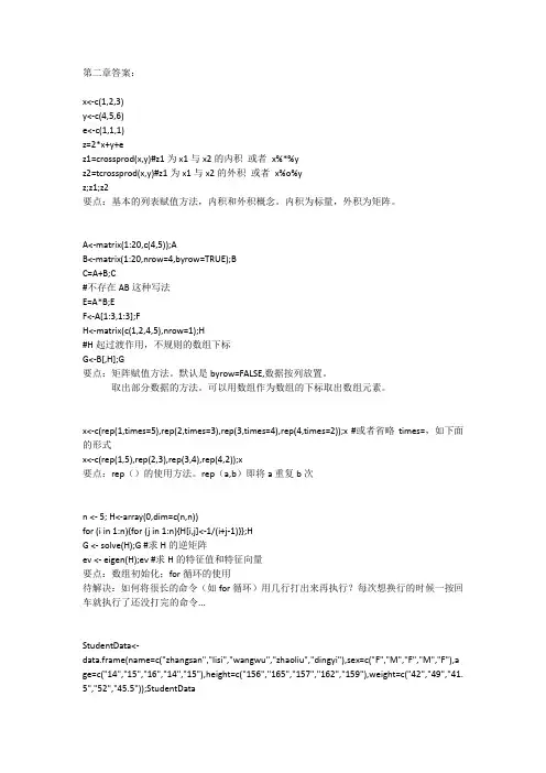
第二章答案：x<-c(1,2,3)y<-c(4,5,6)e<-c(1,1,1)z=2*x+y+ez1=crossprod(x,y)#z1为x1与x2的内积或者x%*%yz2=tcrossprod(x,y)#z1为x1与x2的外积或者x%o%yz;z1;z2要点：基本的列表赋值方法，内积和外积概念。

内积为标量，外积为矩阵。

A<-matrix(1:20,c(4,5));AB<-matrix(1:20,nrow=4,byrow=TRUE);BC=A+B;C#不存在AB这种写法E=A*B;EF<-A[1:3,1:3];FH<-matrix(c(1,2,4,5),nrow=1);H#H起过渡作用，不规则的数组下标G<-B[,H];G要点：矩阵赋值方法。

默认是byrow=FALSE,数据按列放置。

取出部分数据的方法。

可以用数组作为数组的下标取出数组元素。

x<-c(rep(1,times=5),rep(2,times=3),rep(3,times=4),rep(4,times=2));x #或者省略times=，如下面的形式x<-c(rep(1,5),rep(2,3),rep(3,4),rep(4,2));x要点：rep（）的使用方法。

rep（a,b）即将a重复b次n <- 5; H<-array(0,dim=c(n,n))for (i in 1:n){for (j in 1:n){H[i,j]<-1/(i+j-1)}};HG <- solve(H);G #求H的逆矩阵ev <- eigen(H);ev #求H的特征值和特征向量要点：数组初始化；for循环的使用待解决：如何将很长的命令（如for循环）用几行打出来再执行？每次想换行的时候一按回车就执行了还没打完的命令...StudentData<-data.frame(name=c("zhangsan","lisi","wangwu","zhaoliu","dingyi"),sex=c("F","M","F","M","F"),a ge=c("14","15","16","14","15"),height=c("156","165","157","162","159"),weight=c("42","49","41. 5","52","45.5"));StudentData要点：数据框的使用待解决：SSH登陆linux服务器中文显示乱码。

R语言数据分析与统计建模入门指南Chapter 1: Introduction to R Programming LanguageR is a powerful programming language and software environment for statistical computing and graphics. It provides a wide range of statistical and graphical techniques, making it a popular choice for data analysis and statistical modeling. In this chapter, we will introduce the basics of R programming language and its features.1.1 Installing and Setting up RTo get started with R, you need to install it on your computer. R is available for Windows, macOS, and Linux operating systems. Once installed, you can launch the R console or RStudio, which is an integrated development environment (IDE) for R. RStudio provides a user-friendly interface for writing code, managing files, and visualizing data.1.2 Basic R SyntaxR uses a combination of functions, operators, and variables to perform calculations and manipulate data. The basic syntax of R is similar to other programming languages. For example, you can use the assignment operator ( <- ) to assign a value to a variable, or use arithmetic operators (+, -, *, /) to perform calculations.1.3 Data Types in RR supports various data types, including numeric, character, logical, and complex. Numeric data types represent real numbers, character data types store text, logical data types are used to represent logical values (TRUE or FALSE), and complex data types store complex numbers.1.4 Data Structures in RR provides several built-in data structures for storing and organizing data. These include vectors, matrices, data frames, and lists. Vectors are one-dimensional arrays that can store multiple values of the same data type. Matrices are two-dimensional arrays with rows and columns. Data frames are similar to tables in a relational database, and lists can store different types of objects.Chapter 2: Data Import and Manipulation in RIn this chapter, we will focus on how to import data from different file formats into R and perform data manipulation tasks.2.1 Importing Data from CSV FilesCSV (Comma-Separated Values) files are a common format for storing tabular data. R provides functions like read.csv() and read.csv2() to import data from CSV files. These functions automatically detect the delimiters and create data frames in R.2.2 Working with Data FramesData frames are a popular data structure in R. They are similar to tables in a database, with rows and columns. In this section, we will explore various operations that can be performed on data frames, such as subsetting, merging, and sorting.2.3 Data Cleaning and PreprocessingBefore starting any analysis, it is essential to clean and preprocess the data. R offers a wide range of functions and packages for data cleaning, such as removing missing values, handling outliers, and transforming variables. We will explore some commonly used techniques in this section.Chapter 3: Exploratory Data AnalysisExploratory Data Analysis (EDA) is a crucial step in data analysis. It involves summarizing and visualizing the main characteristics of the data. In this chapter, we will learn different techniques to explore and visualize the data using R.3.1 Descriptive StatisticsDescriptive statistics provide summary measures that describe the central tendency, variability, and distribution of the data. R provides functions like mean(), median(), and sd() to calculate these statistics. We will also cover graphical techniques, such as histograms and box plots.3.2 Data VisualizationR offers a rich set of packages for data visualization. We will explore popular packages like ggplot2, which provides a flexible and powerful grammar for creating elegant graphics. We will cover different types of plots, such as scatter plots, bar plots, and density plots.Chapter 4: Statistical Modeling in RStatistical modeling involves building mathematical models to describe and analyze relationships between variables. In this chapter, we will cover some fundamental statistical modeling techniques using R.4.1 Regression AnalysisRegression analysis is a statistical technique used to model the relationship between a dependent variable and one or more independent variables. R provides various functions for fitting linear regression models, such as lm() and glm(). We will learn how to interpret the regression models and assess their goodness of fit.4.2 Hypothesis TestingHypothesis testing is a statistical method used to make inferences about populations based on sample data. R provides functions liket.test() and prop.test() to perform hypothesis tests for means and proportions, respectively. We will discuss the steps involved in hypothesis testing and interpret the results.4.3 ANOVA and Chi-Square TestANOVA (Analysis of Variance) and Chi-Square tests are commonly used statistical tests in various research areas. R provides functions like aov() and chisq.test() to perform these tests. We will learn how to conduct ANOVA tests for comparing means across groups and Chi-Square tests for testing associations between categorical variables.ConclusionIn this introductory guide to R programming language for data analysis and statistical modeling, we covered the basics of R syntax, data types, data structures, import/export, data manipulation, exploratory data analysis, and statistical modeling techniques. R offers a wide range of capabilities for analyzing and visualizing data, making it an essential tool for data scientists and statisticians. With practice and further exploration of R's vast library of packages, you can deepen your knowledge and become proficient in using R for data analysis and statistical modeling.。

R软件介绍(4)：R统计作图金林中南财经政法大学统计系jinlin82@2017年11月4日Outline1简介2高级绘图命令3低级绘图函数4图形参数5网格作图6图形管理简介1简介简介2高级绘图命令3低级绘图函数4图形参数5网格作图6图形管理例子1尝试以下代码: 1demo(graphics) 2demo(persp)3library(lattice) 4demo(lattice)命令种类1高级绘图命令在图形设备上产生一个新的图区，它可能包括坐标轴，标签，标题等等2低级绘图命令在一个已经存在的图上加上更多的图形元素，如额外的点，线和标签3图形参数图形参数可以被修改从而定制图形环境4网格作图命令使用grid和lattice进行面板作图5图形设备管理命令通过设备管理命令来保存R图形高级绘图命令1简介2高级绘图命令plot函数hist函数pairs函数coplot函数其他常见高级函数3低级绘图函数4图形参数5网格作图plot函数使用方法1是R里面最常用的一个图形函数2是一个泛型函数：产生的图形依赖于第一个参数的类型或者类3使用方法1plot(x):以x的元素值为纵坐标、以序号为横坐标绘图2plot(x,y):x(在x-轴上)与y(在y-轴上)的二元作图3plot(y x):x(在x-轴上)与y(在y-轴上)的二元作图4plot(DF):矩阵散点图参数作用add=F如果是TRUE，叠加图形到前一个图上（如果有的话）axes=T如果是FALSE，不绘制轴与边框type="p"指定图形的类型，"p":点，"l":线，"b":点连线，"o":同上，但是线在点上xlim=,ylim=指定轴的上下限，例如xlim=c(1,10)xlab=,ylab=坐标轴的标签，必须是字符型值main=,sub=指定主标题和副标题，必须是字符型值1plot(1:10)2a<-1:103b<-11:204plot(a,b)5plot(b~a)6A<-matrix(1:20,nrow=10)7plot(A)8plot(1:10,type="l")9plot(b~a,type="o",xlim=c(0,12),ylim=c(0,22),10xlab="x轴",ylab="y轴")11setwd("C:/Works/Teaching/2015年2月--统计系软件培训/report/lecture4/") 12GDPdata<-read.csv(file="../../data/GDP.csv")13str(GDPdata)#查看GDPdata的结构14plot(GDPdata[,c("GDP","Labor","Kapital","Technology")])hist函数1x的频率直方图2例子1#Make some sample dat2x<-rnorm(100)3#Calculate and plot the two histograms4hcum<-h<-hist(x,plot=FALSE)5hcum$counts<-cumsum(hcum$counts)6plot(hcum,main="")7plot(h,add=T,col="grey")8#Plot the density and cumulative density9d<-density(x)10lines(x=d$x,y=d$y*length(x)*diff(h$breaks)[1],lwd=1,col="red")11lines(x=d$x,y=cumsum(d$y)/max(cumsum(d$y))*length(x),lwd=1,col="blue")hist 例子图形F r e q u e n c y020*********pairs函数1作多个变量的散点图矩阵.2参数为数据框对象.3效果与plot函数使用数据框参数效果相同1pairs(GDPdata[,c("GDPRealRate","Labor","KR","Technology","CPI")]) 2plot(GDPdata[,c("GDPRealRate","Labor","KR","Technology","CPI")]) 3dev.off()pairs函数：panel参数1默认散点图矩阵存在的问题：空间比较浪费，没有揭示更多内容1矩阵图中上三角和下三角的内容雷同2矩阵对角线只有变量的名称2解决方法：使用panel参数:1panel定义每个矩阵元素图中的图形，默认为散点图2lower.panel定义下三角矩阵的图形，默认为散点图3upper.panel定义上三角矩阵的图形，默认为散点图4diag.panel定义对角线的图形，默认为不绘制图形3上面几个panel参数应设置为作图函数，可以为已有的作图函数，也可以自己定义。

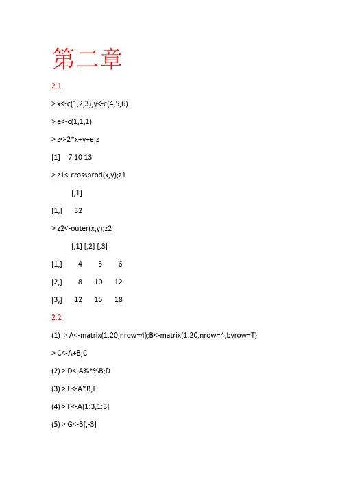
第二章2.1> x<-c(1,2,3);y<-c(4,5,6)> e<-c(1,1,1)> z<-2*x+y+e;z[1] 7 10 13> z1<-crossprod(x,y);z1[,1][1,] 32> z2<-outer(x,y);z2[,1] [,2] [,3][1,] 4 5 6[2,] 8 10 12[3,] 12 15 182.2(1)> A<-matrix(1:20,nrow=4);B<-matrix(1:20,nrow=4,byrow=T) > C<-A+B;C(2)> D<-A%*%B;D(3)> E<-A*B;E(4)> F<-A[1:3,1:3](5)> G<-B[,-3]> x<-c(rep(1,5),rep(2,3),rep(3,4),rep(4,2));x2.4> H<-matrix(nrow=5,ncol=5)> for (i in 1:5)+ for(j in 1:5)+ H[i,j]<-1/(i+j-1)（1）> det(H)（2）> solve(H)（3）> eigen(H)2.5> studentdata<-data.frame(姓名=c('张三','李四','王五','赵六','丁一')+ ,性别=c('女','男','女','男','女'),年龄=c('14','15','16','14','15'),+ 身高=c('156','165','157','162','159'),体重=c('42','49','41.5','52','45.5')) 2.6> write.table(studentdata,file='student.txt')> write.csv(studentdata,file='student.csv')2.7count<-function(n){if (n<=0)print('要求输入一个正整数')repeat{if (n%%2==0)n<-n/2elsen<-(3*n+1)if(n==1)break}print('运算成功')}}第三章3.1首先将数据录入为x。

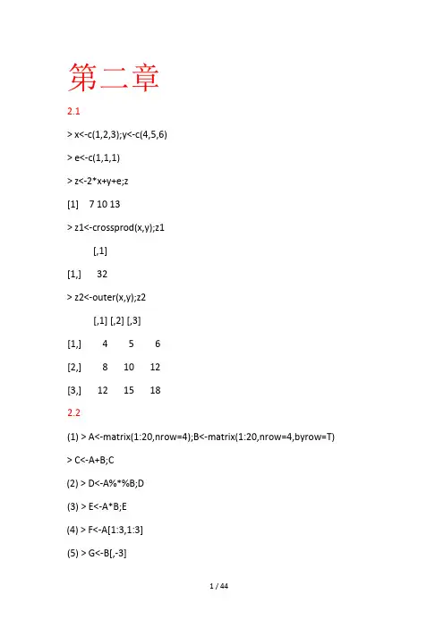
第二章2.1> x<-c(1,2,3);y<-c(4,5,6)> e<-c(1,1,1)> z<-2*x+y+e;z[1] 7 10 13>z1<-crossprod(x,y);z1[,1][1,] 32>z2<-outer(x,y);z2[,1] [,2] [,3][1,] 4 5 6[2,] 8 10 12[3,] 12 15 182.2(1) > A<-matrix(1:20,nrow=4);B<-matrix(1:20,nrow=4,byrow=T) >C<-A+B;C(2) > D<-A%*%B;D(3) > E<-A*B;E(4) > F<-A[1:3,1:3](5) > G<-B[,-3]2.3>x<-c(rep(1,5),rep(2,3),rep(3,4),rep(4,2));x2.4>H<-matrix(nrow=5,ncol=5)>for (i in 1:5)+ for(j in 1:5)+ H[i,j]<-1/(i+j-1)（1）> det(H)（2）> solve(H)（3）> eigen(H)2.5>studentdata<-data.frame(姓名=c('张三','李四','王五','赵六','丁一') + ,性别=c('女','男','女','男','女'),年龄=c('14','15','16','14','15'),+ 身高=c('156','165','157','162','159'),体重=c('42','49','41.5','52','45.5')) 2.6>write.table(studentdata,file='student.txt')>write.csv(studentdata,file='student.csv')2.7count<-function(n){if (n<=0)print('要求输入一个正整数')else{ repeat{if (n%%2==0)n<-n/2elsen<-(3*n+1)if(n==1)break}print('运算成功')}}第三章3.1首先将数据录入为x。

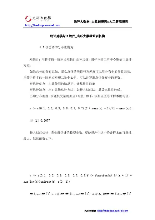
统计建模与R软件_光环大数据培训机构4.1设总体的分布密度为矩估计：用样本的一阶原点矩估计总体均值；用样本的二阶中心矩估计总体方差。

如果总体的分布已知，那么总体的均值和方差就可以用分布中的参数表示，再等于样本的一阶原点矩和二阶中心矩，可以计算出总体分布中的参数。

矩估计优点：在其能用的情况下，计算往往简单矩估计缺点：相对其他估计方法，如极大似然法，其效率往往较低。

已知分布密度，求随机变量的期望（均值）如下，该期望值等于样本的均值：x <- c(0.1, 0.2, 0.9, 0.8, 0.7, 0.7)(2 * mean(x) - 1)/(1 - mean(x)) ## [1] 0.3077极大似然估计：我们所估计的模型参数，要使得产生这个给定样本的可能性最大。

似然函数如下：x <- c(0.1, 0.2, 0.9, 0.8, 0.7, 0.7)f <- function(a) 6/(a + 1) + sum(log(x))uniroot(f, c(0, 1))## $root## [1] 0.2112## ## $f.root## [1] -3.845e-05## ## $iter## [1]5## ## $estim.prec## [1] 6.104e-05root为估计值，iter为迭代次数，optimize函数也可以用来求解方程。

λ^=n∑ni=1xix <- c(rep(5, 365), rep(15, 245), rep(25, 150), rep(35, 100), rep(45, 70), rep(55, 45), rep(65, 25))1000/sum(x)## [1] 0.05x <- c(rep(0, 17), rep(1, 20), rep(2, 10), rep(3, 2), rep(4, 1), rep(5, 0), rep(6, 0))## 得到$/lambda$的估计值mean(x)## [1] 1x(0)=(0.5,−2)T.# 目标函数obj <- function(x) { f <- c(-13 + x[1] + ((5 - x[2])* x[2] - 2) * x[2], -29 + x[1] + ((x[2] + 1) * x[2] - 14) * x[2]) sum(f^2)}x0 <- c(0.5, -2)nlm(obj, x0)## $minimum## [1] 48.98## ## $estimate## [1] 11.4128 -0.8968## ## $gradient## [1] 1.415e-08 -1.435e-07## ## $code## [1] 1## ## $iterations## [1] 16# 最优目标值为 $minimum 48.984.5正常人的脉搏平均每分钟72次，某医生测得10例四乙基铅中毒患者的脉搏数（次/分）如下：54 67 68 78 70 66 67 70 65 69已知人的脉搏次数服从正态分布，试计算这10名患者平均脉搏次数的点估计和95的区间估计。

统计建模与R软件课程报告对某地区农业生态经济的发展状况作主成分分析主成分分析的主要目的是希望用较少的变量去解释原来资料中的大部分变异，将我们手中许多相关性很高的变量转化成彼此相关独立或不相关的变量。

通常是选出比原始变量个数少，又能解释大部分资料中的变异的几个新变量，即所谓主成分，并用以解释资料的综合性指标。

也就是说，主成分分析实际上是一种降维方法。

关键词：主成分分析相关矩阵相关R函数1 绪论 (2)1.1主成分方法简介 (2)2总体主成分 (2)2.1主成分的定义与导出 (2)2.2主成分的性质 (3)2.3从相关矩阵出发求主成分 (5)2.4相关的R函数 (6)3数据模拟 (7)4结论及对该模型的评价 (12)参考文献 (12)1.1主成分方法简介主成分分析(principal component analysis )是将多个指标化为少数几个 综合指标的一种统计分析方法，由Pearson( 1901)提出，后来被Hotelling ( 1933) 发展了。

主成分分析是一种通过降维技术把多个变量化成少数几个主成分的方法。

这些主成分能够反映原始变量的绝大部分信息，它们通常表示为原始变量的线性 组合。

主成分分析也称主分量分析， 旨在利用降维的思想，把多指标转化为少数几个综合指标。

在实证问题研究中，为了全面、系统地分析问题，我们必须考虑众多影响因素。

这些涉及的 因素一般称为指标，在多元统计分析中也称为变量。

因为每个变量都在不同程度上反映了所研究问题的某些信息，并且指标之间彼此有一定的相关性，因而所得的统计数据反映的信息在一定程度上有重叠。

在用统计方法研究多变量问题时，变量太多会增加计算量和增加分析 问题的复杂性，人们希望在进行定量分析的过程中，涉及的变量较少，得到的信息量较多。

主成分分析正是适应这一要求产生的，是解决这类题的理想工具。

2总体主成分2.1主成分的定义与导出易见var( ZJ 二 a TZa i , i=1,2,,p,我们希望乙的方差达到最大，即a 1是约束优化问题max a T las.ta T a = 11绪论设x 是p 维随机变量，并假设艺二var(X )。

如何使用R语言进行统计建模与数据分析R语言是一种功能强大的编程语言和开源软件环境，被广泛应用于统计学、数据分析和机器学习等领域。

本文将介绍如何使用R语言进行统计建模与数据分析，内容包括：数据导入与处理、探索性数据分析、统计建模以及结果解释与可视化等方面。

第一章：数据导入与处理在进行统计建模与数据分析之前，首先需要将数据导入到R环境中，并进行必要的数据处理。

R语言提供了多种导入数据的函数，如read.csv()、read.table()等，可以读取包括CSV、Excel、文本文件等多种格式的数据。

在导入数据后，需要对数据进行初步处理，包括数据清洗、缺失值处理以及数据格式转换等。

R语言提供了如na.omit()、is.na()等函数用于处理缺失值，而通过转换函数如as.numeric()、as.character()等可以将数据类型转换成所需的类型。

第二章：探索性数据分析在进行统计建模前，我们需要对数据进行探索性的数据分析，了解数据的基本特征和分布情况，并确定适合使用的统计模型。

探索性数据分析的常用方法包括描述性统计、数据可视化和相关性分析等。

R语言提供了丰富的函数和包来支持这些分析，如summary()、hist()、boxplot()等。

通过这些函数和包，我们可以计算数据的均值、中位数、方差等统计指标，并绘制直方图、箱线图、散点图等图形来展示数据的分布和变化情况。

第三章：统计建模在进行统计建模时，我们需要根据问题的性质和数据的特点选择适合的统计模型，如线性回归、逻辑回归、决策树、随机森林等。

R语言提供了强大的统计建模包，如stats、glmnet、rpart等，可以帮助我们实现各种统计建模算法。

在建立模型之前，我们需要将数据集划分为训练集和测试集，以便进行模型拟合和验证。

R语言提供了如caret、caTools等包，可以方便地进行数据集划分。

然后，我们可以使用模型拟合函数（如lm()、glm()等）对训练集进行拟合，得到模型的参数估计值。

如何使用R进行数据分析和统计建模R语言是一种强大的开源编程语言，广泛应用于数据分析和统计建模领域。

它提供了丰富的函数和包，可以帮助研究人员和数据分析师处理和分析各种类型的数据。

本文将介绍如何使用R进行数据分析和统计建模的基本步骤和技巧。

一、数据准备在开始数据分析之前，首先需要准备好数据。

数据可以来自各种渠道，如Excel表格、数据库、文本文件等。

在R中，可以使用read.csv()、read.table()等函数将数据导入到R中。

导入数据后，可以使用head()函数查看数据的前几行，以确保数据导入正确。

二、数据清洗数据清洗是数据分析的重要步骤之一。

在清洗数据时，需要处理缺失值、异常值、重复值等问题。

R提供了一系列函数和包，如na.omit()、complete.cases()、duplicated()等，可以帮助我们进行数据清洗。

例如，可以使用na.omit()函数删除包含缺失值的观测，使用duplicated()函数删除重复的观测。

三、数据探索数据探索是了解数据的基本特征和分布的过程。

在R中，可以使用summary()函数查看数据的基本统计信息，如均值、中位数、最小值、最大值等。

另外，可以使用hist()、boxplot()等函数绘制直方图、箱线图等图形，帮助我们更直观地了解数据的分布和异常值。

四、数据可视化数据可视化是将数据转化为图形或图表的过程，可以帮助我们更好地理解数据。

R提供了丰富的绘图函数和包，如ggplot2、lattice等。

使用这些函数和包，可以绘制各种类型的图形，如散点图、折线图、饼图等。

通过数据可视化，我们可以发现数据中的模式、趋势和关系，为后续的统计建模提供参考。

五、统计建模统计建模是根据数据进行模型构建和预测的过程。

R提供了多种统计建模的函数和包，如lm()、glm()、randomForest等。

在进行统计建模时，需要选择合适的模型和变量，并进行模型拟合和评估。

通过模型拟合，我们可以了解变量之间的关系和影响，通过模型评估，我们可以判断模型的拟合优度和预测能力。

RStudio统计编程软件使用教程第一章：RStudio简介RStudio是一个强大的开源集成开发环境（IDE），用于进行统计分析和数据可视化。

它是基于R语言的核心并提供了一些方便的功能和工具，使得数据科学家和统计分析人员能够更轻松地处理和分析数据。

在本章中，我们将介绍RStudio的基本功能和界面。

RStudio的界面分为四个主要区域：源代码编辑器、工作区、控制台和文件相关工具。

源代码编辑器是主要工作区，用于编写和调试R代码。

工作区可用于查看和管理数据、环境变量和图形等对象。

控制台是R解释器的主要接口，可用于执行代码和查看输出。

文件相关工具提供了文件浏览器、包管理器和版本控制等功能。

第二章：RStudio的安装和配置在本章中，我们将介绍RStudio的安装和配置步骤。

首先，您需要从RStudio的官方网站（https：///）下载适合您操作系统的安装程序。

然后，按照安装向导的指示进行安装。

在完成安装后，打开RStudio并进行必要的配置。

在配置RStudio之前，您需要安装R语言环境。

可以从R官方网站（https：///）下载适合您操作系统的R安装程序。

安装R后，打开RStudio并进行以下配置：1. 设置默认工作目录：通过点击“工具”>“全局选项”>“一般”来设置默认工作目录。

选择您想要的目录，并确保在启动RStudio时自动设置。

2. 配置R库路径：通过点击“工具”>“全局选项”>“Packages”来配置R库路径。

您可以添加多个路径，以便RStudio能够搜索和加载您的R包。

3. 配置R解释器：通过点击“工具”>“全局选项”>“R”来配置R 解释器。

选择正确的R解释器路径，以确保RStudio正确连接到R 语言环境。

第三章：RStudio的基本操作在本章中，我们将介绍RStudio的基本操作。

1. 创建和运行脚本：在源代码编辑器中，使用新建文件按钮或快捷键Ctrl + Shift + N来创建一个新的脚本文件。