matlab潮流计算工具箱使用手册
- 格式:pdf
- 大小:3.04 MB
- 文档页数:40
MATLAB机器学习工具箱的使用方法1. 引言在现代科技发展的背景下,机器学习在各个领域中的应用越来越广泛。
而MATLAB作为一款功能强大的数学软件,其机器学习工具箱为用户提供了丰富的算法和工具,方便快捷地进行机器学习任务。
本文将详细介绍MATLAB机器学习工具箱的使用方法,帮助读者更好地利用这个工具箱进行数据分析、模型训练和结果评估等任务。
2. 数据预处理在进行机器学习任务之前,首先需要对数据进行预处理。
MATLAB机器学习工具箱提供了多种数据预处理的方法和函数,如数据清洗、特征选择、数据变换等。
可以使用`preprocess`函数对数据进行缺失值处理,使用`featureselect`函数进行特征选择,或者使用`datapreprocessing`函数进行数据变换。
通过这些预处理的方法,可以使得数据更好地适用于后续的机器学习算法。
3. 特征工程特征工程是机器学习中一个重要的环节,它的目的是将原始数据转换为能够更好地反映问题特点的特征。
MATLAB机器学习工具箱提供了丰富的特征工程方法和函数,如特征提取、特征转换和特征选择等。
可以使用`featureextract`函数对原始数据进行特征提取,使用`featuretransform`函数进行特征转换,或者使用`featureselect`函数进行特征选择。
这些方法和函数的灵活使用可以帮助用户更好地理解数据并选择合适的特征。
4. 模型选择与训练在进行机器学习任务的过程中,选择适合问题的机器学习模型是非常重要的。
MATLAB机器学习工具箱提供了多种常见的机器学习模型,如线性回归、决策树、支持向量机等。
可以使用`fitmodel`函数来选择和训练机器学习模型。
用户可以根据具体的问题需求选择合适的模型,并通过调整模型参数来优化模型性能。
5. 模型评估与调优在完成模型的训练之后,需要对模型的性能进行评估和调优。
MATLAB机器学习工具箱提供了多种模型评估的方法和函数,如交叉验证、ROC曲线分析、精确度和召回率等。
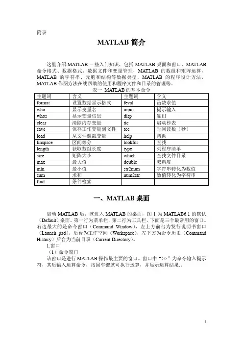
附录MATLAB简介这里介绍MATLAB一些入门知识,包括MATLAB桌面和窗口,MATLAB 命令格式、数据格式、数据文件和变量管理,MATLAB的数组和矩阵运算,MATLAB的字符串、元胞和结构等数据类型,MATLAB的程序设计方法,MATLAB作图方法在线帮助的使用和程序文件和目录的管理等。
一、MATLAB桌面启动MATLAB后,就进入MATLAB的桌面,图1为MATLAB6.1的默认(Default)桌面。
第一行为菜单栏,第二行为工具栏,下面是三个最常用的窗口。
右边最大的是命令窗口(Command Window),左上方前台为发行说明书窗口(Launch pad),后台为工作空间(Workspace),左下方为命令历史(Command History)后台为当前目录(Current Directory)。
1.窗口(1)命令窗口该窗口是进行MATLAB操作最主要的窗口。
窗口中“>>”为命令输入提示符,其后输入运算命令,按回车键就可执行运算,并显示运算结果.。
图1 (2)发行说明书窗口发行说明书窗口是MATLAB 所特有的,用来说明用户所拥有的Mathworks 公司产品的工具包、演示以及帮助信息。
(3)工作空间在默认桌面,位于左上方窗口前台,列出内存中MATLAB 工作空间的所有变量的变量名、尺寸、字节数。
用鼠标选中变量,击右键可以打开、保存、删除、绘图等操作。
(4)当前目录在默认桌面,位于左下方窗口后台,用鼠标点击可以切换到前台。
该窗口列出当前目录的程序文件(.m )和数据文件(.mat )等。
用鼠标选中文件,击右键可以进行打开、运行、删除等操作。
(5)命令历史(Command History )该窗口列出在命令窗口执行过的MATLAB 命令行的历史记录。
用鼠标选中命令行,击右键可以进行复制、执行(Evaluate Selection )、删除等操作。
除上述窗口外,MATLAB 常用窗口还有编程器窗口、图形窗口等。
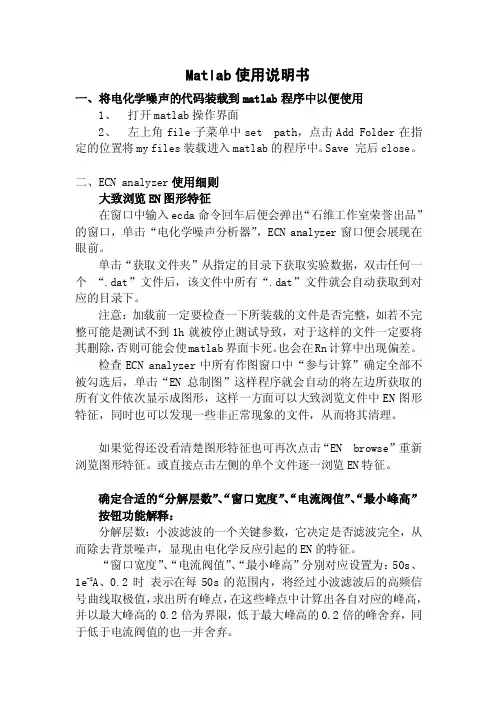
Matlab使用说明书一、将电化学噪声的代码装载到matlab程序中以便使用1、打开matlab操作界面2、左上角file子菜单中set path,点击Add Folder在指定的位置将my files装载进入matlab的程序中。
Save 完后close。
二、ECN analyzer使用细则大致浏览EN图形特征在窗口中输入ecda命令回车后便会弹出“石维工作室荣誉出品”的窗口,单击“电化学噪声分析器”,ECN analyzer窗口便会展现在眼前。
单击“获取文件夹”从指定的目录下获取实验数据,双击任何一个“.dat”文件后,该文件中所有“.dat”文件就会自动获取到对应的目录下。
注意:加载前一定要检查一下所装载的文件是否完整,如若不完整可能是测试不到1h就被停止测试导致,对于这样的文件一定要将其删除,否则可能会使matlab界面卡死。
也会在Rn计算中出现偏差。
检查ECN analyzer中所有作图窗口中“参与计算”确定全部不被勾选后,单击“EN总制图”这样程序就会自动的将左边所获取的所有文件依次显示成图形,这样一方面可以大致浏览文件中EN图形特征,同时也可以发现一些非正常现象的文件,从而将其清理。
如果觉得还没看清楚图形特征也可再次点击“EN browse”重新浏览图形特征。
或直接点击左侧的单个文件逐一浏览EN特征。
确定合适的“分解层数”、“窗口宽度”、“电流阀值”、“最小峰高”按钮功能解释:分解层数:小波滤波的一个关键参数,它决定是否滤波完全,从而除去背景噪声,显现由电化学反应引起的EN的特征。
“窗口宽度”、“电流阀值”、“最小峰高”分别对应设置为:50s、1e-8A、0.2时表示在每50s的范围内,将经过小波滤波后的高频信号曲线取极值,求出所有峰点,在这些峰点中计算出各自对应的峰高,并以最大峰高的0.2倍为界限,低于最大峰高的0.2倍的峰舍弃,同于低于电流阀值的也一并舍弃。
所以“窗口宽度”、“电流阀值”、“最小峰高”这三个参数决定最终选取峰的数目,为了保证所选峰合理性,可以适当调整上述三个参数,如将分解层数适当调大,电流阀值降低、最小峰高也降低便可将一些小峰选入其中,但实际应用中,太小的峰没有什么意义。
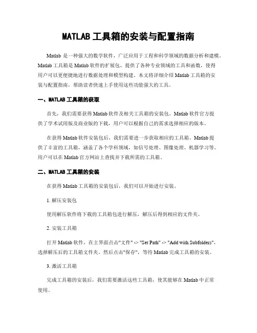
MATLAB工具箱的安装与配置指南Matlab是一种强大的数学软件,广泛应用于工程和科学领域的数据分析和建模。
Matlab工具箱是Matlab软件的扩展包,提供了各种专业领域的工具和函数,使得用户可以更便捷地进行数据处理和模型构建。
本文将详细介绍Matlab工具箱的安装与配置指南,帮助读者快速上手使用这些功能强大的工具。
一、MATLAB工具箱的获取首先,我们需要获得Matlab软件及相关工具箱的安装包。
Matlab软件官方提供了学术试用版及商业版的下载,用户可以根据自己的需求选择相应的版本。
在获得Matlab软件安装包后,我们需要进一步获取相应的工具箱。
Matlab提供了丰富的工具箱,涵盖了各个学科领域,如信号处理、图像处理、机器学习等。
用户可以在Matlab官方网站上查找并下载所需的工具箱。
二、MATLAB工具箱的安装在获得Matlab工具箱的安装包后,我们可以开始进行安装。
1. 解压安装包使用解压软件将下载的工具箱包进行解压,解压后得到相应的文件夹。
2. 安装工具箱打开Matlab软件,在主界面点击"文件" -> "Set Path" -> "Add with Subfolders",选择解压后的工具箱文件夹。
然后点击"保存",等待Matlab完成工具箱的安装。
3. 激活工具箱完成工具箱的安装后,我们需要激活这些工具箱,使其能够在Matlab中正常使用。
在Matlab主界面点击"Home" -> "Help" -> "Licensing",将打开"Licensing"窗口。
选择"Activate Software",输入Matlab账户信息,点击"Next",根据指引完成激活过程。

matlab tmd潮汐使用方法下载提示:该文档是本店铺精心编制而成的,希望大家下载后,能够帮助大家解决实际问题。
文档下载后可定制修改,请根据实际需要进行调整和使用,谢谢!本店铺为大家提供各种类型的实用资料,如教育随笔、日记赏析、句子摘抄、古诗大全、经典美文、话题作文、工作总结、词语解析、文案摘录、其他资料等等,想了解不同资料格式和写法,敬请关注!Download tips: This document is carefully compiled by this editor. I hope that after you download it, it can help you solve practical problems. The document can be customized and modified after downloading, please adjust and use it according to actual needs, thank you! In addition, this shop provides you with various types of practical materials, such as educational essays, diary appreciation, sentence excerpts, ancient poems, classic articles, topic composition, work summary, word parsing, copy excerpts, other materials and so on, want to know different data formats and writing methods, please pay attention!MATLAB TMD潮汐使用方法引言在海洋工程和地球物理学领域,潮汐是一项重要的研究对象。

电力系统大作业——用matlab潮流计算郭尚坤08292007 电气0809班%主程序:[dfile,pathname]=uigetfile('ieee14.m','Select Data File');if pathname==0error('you must select a valid data file')elselfile=length(dfile);% strip off .meval(dfile(1:lfile-2)); %打开数据文件endglobal n;global m;[nb,mb]=size(bus); %节点重新编号[nl,ml]=size(line);nSW=0; % 平衡节点数目nPV=0; % PV节点数目nPQ=0; % PQ节点数目for i=1:nb, % nb为总节点数type=bus(i,6);if type==3,nSW=nSW+1; % 统计平衡节点数目SW(nSW,:)=bus(i,:);elseif type==2,nPV=nPV+1; % 统计PV节点数目PV(nPV,:)=bus(i,:);elsenPQ=nPQ+1; % 统计PQ节点数目PQ(nPQ,:)=bus(i,:);endend;bus=[PQ;PV;SW];newbus=[1:nb]';f=bus(:,1);nodenum=[newbus bus(:,1)];bus(:,1)=newbus;for i=1:nlfor j=1:2for k=1:nbif line(i,j)==nodenum(k,2)line(i,j)=nodenum(k,1);breakendendendendK=0; %迭代次数初值Kmax=10; %最大迭代次数eps1=1.0e-10;eps2=1.0e-10;m=nPQ;n=nb;Um=eye(m,m);myf=fopen('output1.dat','w');for K=1:Kmaxfor i=1:mfor j=1:mif i==jUm(i,j)=bus(i,2);endendendb=dPQ(Y,bus);C=jac(bus,Y);dX=C\b';dx=dX';[nx,mx]=size(dx);for i=1:n-1 %计算相角bus(i,3)=bus(i,3)-dX(i,1);endB=dx(nx,n:mx)*Um; %计算电压差bus(1:m,2)=bus(1:m,2)-B'; %计算电压值dx(nx,n:mx)=B;fprintf(myf,'--第%d次迭代时雅可比矩阵--',K)fprintf(myf, '\n');for i=1:(n+m-1)for j=1:(n+m-1)fprintf(myf,'%8.6f', C(i,j));fprintf(myf, ' ');endfprintf(myf, '\n');endfprintf(myf,'--第%d次迭代时dPQ的误差--',K)fprintf(myf, '\n');for i=1:(n+m-1)fprintf(myf,'%8.6e', b(1,i));fprintf(myf, '\n');endfprintf(myf, '\n');fprintf(myf,'--第%d次迭代时dx(误差)--',K)fprintf(myf, '\n');for i=1:(n+m-1)fprintf(myf,'%8.6e', dX(i,1));fprintf(myf, '\n');fprintf(myf, '\n');fprintf(myf,'第%d次迭代后节点电压(仅PQ节点)',K)fprintf(myf, '\n');for i=1:mfprintf(myf,'%8.6f', bus(i,2));fprintf(myf, '\n');endfprintf(myf, '\n');fprintf(myf,'第%d次迭代后相角(角度)',K)fprintf(myf, '\n');for i=1:nfprintf(myf,'%8.6f', bus(i,3)*180/pi);fprintf(myf, '\n');endfprintf(myf, '\n');if (max(abs(dx))<eps1)&(max(abs(b))<eps2) %判断是否达到计算精度break;endend%计算功率P1=0;T=0; %计算平衡节点的有功for j=1:nT=bus(n,2)*bus(j,2)*(real(Y(n,j))*cos(bus(n,3)-bus(j,3))+imag(Y(n,j))*sin(bus(n,3)-bus(j,3)));P1=P1+T;endbus(n,4)=P1;for k=m+1:n %计算PV节点、平衡节点的无功Q1=0;T=0;for j=1:nT=bus(k,2)*bus(j,2)*(real(Y(k,j))*sin(bus(k,3)-bus(j,3))-imag(Y(k,j))*cos(bus(k,3)-bus(j,3)));Q1=Q1+T;endbus(k,5)=Q1;endbus(:,1)=f; %换回各节点、支路的初始编号r=zeros(1,mb);for t=1:nfor l=t+1:nif bus(t,1)>bus(l,1)r=bus(t,:);bus(t,:)=bus(l,:);bus(l,:)=r;endendendfor i=1:nlfor j=1:2for k=1:nbif line(i,j)==nodenum(k,1)breakendendendendfclose(myf);Pf=loss(bus,line); %计算支路潮流及损耗%将节点导纳矩阵、节点潮流计算结果写入文件output2myf=fopen('output2.dat','w');fprintf(myf, '--节点导纳矩阵--\n');for k=1:nfor j=1:nfprintf(myf,'%8.6f', real(Y(k,j)));fprintf(myf, '+i*');fprintf(myf,'%8.6f', imag(Y(k,j)));fprintf(myf, ' ');endfprintf(myf, '\n');endfprintf(myf, '------------------牛顿-拉夫逊法潮流计算结果-------------\n');fprintf(myf, '------------节点计算结果------------\n');fprintf(myf, '-- 节点节点电压节点相角注入有功功率(P)注入无功功率(Q) 类型--\n');for l=1:nbfor j=1:mbif j==1|j==6fprintf(myf, ' %8.1f ', bus(l,j));elseif j==3fprintf(myf, ' %8.6f ', bus(l,j)*180/pi);elsefprintf(myf, ' %8.6f ', bus(l,j));endendfprintf(myf, ' \n');endfprintf(myf, '--支路计算结果--\n');fprintf(myf, '-- 节点(I) 节点(J) 线路功率S(I,J) 线路功率S(J,I) 线路损耗dS(I,J)--\n');for k=1:nlfor j=1:5if j<=2fprintf(myf,'%8.1f ', Pf(k,j));fprintf(myf, ' ');elsefprintf(myf,'%8.6f', real(Pf(k,j)));fprintf(myf, '+i*');fprintf(myf,'%8.6f', imag(Pf(k,j)));endendfprintf(myf, '\n');endfclose(myf);%根据支路参数建立节点导纳矩阵程序:function Y=y(bus,line)%目的:根据支路参数建立节点导纳矩阵%输入:节点参数矩阵--bus;支路参数矩阵--line%输出:节点导纳矩阵--Y[nb,mb]=size(bus);[nl,ml]=size(line);Y=zeros(nb,nb);for k=1:nlI=line(k,1);J=line(k,2);Zt=line(k,3)+j*line(k,4);if Zt==0disp('对地支路');Yt=inf;elseYt=1/Zt;endYm=line(k,5)+j*line(k,6);K=line(k,7);if(K==0)&(J~=0) %普通线路Y(I,I)=Y(I,I)+Yt+Ym;Y(J,J)=Y(J,J)+Yt+Ym;Y(I,J)=Y(I,J)-Yt;Y(J,I)=Y(I,J);endif(K==0)&(J==0) %对地支路K=J=0,R=X=0 Y(I,I)=Y(I,I)+Ym;endif K>0 %K>0时变压器支路Y(I,I)=Y(I,I)+Yt+Ym;Y(J,J)=Y(J,J)+Yt/K^2;Y(I,J)=Y(I,J)-Yt/K;Y(J,I)=Y(I,J);endif K<0 %K<0时变压器支路Y(I,I)=Y(I,I)+Yt+Ym;Y(J,J)=Y(J,J)+Yt*K^2;Y(I,J)=Y(I,J)+Yt*K;endend%形成雅克矩阵程序:function J=jac(bus,Y)%形成雅可比矩阵global n;global m;for i=1:(n-1) %计算PQ、PV节点的有功P1=0;T=0;for j=1:nT=bus(i,2)*bus(j,2)*(real(Y(i,j))*cos(bus(i,3)-bus(j,3))+imag(Y(i,j))*sin(bus(i,3)-bus(j,3)));P1=P1+T;endbus(i,4)=P1;endfor i=1:n-1 %计算PV、PQ节点的无功Q1=0;T=0;for j=1:nT=bus(i,2)*bus(j,2)*(real(Y(i,j))*sin(bus(i,3)-bus(j,3))-imag(Y(i,j))*cos(bus(i,3)-bus(j,3)));Q1=Q1+T;endbus(i,5)=Q1;endfor i=1:n-1 %计算Hfor j=1:n-1if i~=jH(i,j)=-bus(i,2)*bus(j,2)*(real(Y(i,j))*sin(bus(i,3)-bus(j,3))-imag(Y(i,j))*cos(bus(i,3)-bus(j,3)));N(i,j)=-bus(i,2)*bus(j,2)*(real(Y(i,j))*cos(bus(i,3)-bus(j,3))+imag(Y(i,j))*sin(bus(i,3)-bus(j,3)));K(i,j)=bus(i,2)*bus(j,2)*(real(Y(i,j))*cos(bus(i,3)-bus(j,3))+imag(Y(i,j))*sin(bus(i,3)-bus(j,3)));L(i,j)=H(i,j);endendendfor i=1:n-1 %计算Hfor j=1:n-1if j==iH(i,i)=bus(i,5)+imag(Y(i,i))*bus(i,2)^2;N(i,i)=-bus(i,4)-real(Y(i,i))*bus(i,2)^2;K(i,i)=N(i,i)+2*real(Y(i,i))*bus(i,2)^2;L(i,i)=-H(i,i)+2*imag(Y(i,i))*bus(i,2)^2;endendendN=N(1:n-1,1:m);L=L(1:m,1:m);J=[H,N;K,L];%计算dPQ的程序:function dPQ=dPQ(Y,bus)%delP--有功偏差量%delQ--无功偏差量%Y--节点导纳矩阵%bus--节点参数(P,Q,U及相角)矩阵global n;global m;delP=zeros(1,n-1);delQ=zeros(1,m);for i=1:(n-1) %形成delP矩阵(PQ、PV节点)P1=0;T=0;for j=1:nT=bus(i,2)*bus(j,2)*(real(Y(i,j))*cos(bus(i,3)-bus(j,3))+imag(Y(i,j))*sin(bus(i,3)-bus(j,3)));P1=P1+T;enddelP(1,i)=bus(i,4)-P1;endfor i=1:m %形成delQ矩阵(PQ节点)Q1=0;T=0;for j=1:nT=bus(i,2)*bus(j,2)*(real(Y(i,j))*sin(bus(i,3)-bus(j,3))-imag(Y(i,j))*cos(bus(i,3)-bus(j,3)));Q1=Q1+T;enddelQ(1,i)=bus(i,5)-Q1;enddPQ=[delP,delQ];%计算线路损耗、线路潮流程序:function Pf=loss(bus,line)%计算线路损耗、线路潮流[nl,ml]=size(line);Pf=zeros(nl,5);for k=1:nlI=line(k,1);J=line(k,2);Zt=line(k,3)+i*line(k,4);if Zt==0Yt=inf;elseYt=1/Zt;endYm=line(k,5)+i*line(k,6);K=line(k,7);if (K==0)&(J~=0) %普通线路潮流S(I,J)=bus(I,2)^2*(conj(Yt)+conj(Ym))-bus(I,2)*(cos(bus(I,3))+i*sin(bus(I,3)))*bus(J,2)*(cos(bus(J,3))-i*sin(bus(J,3))) *conj(Yt);S(J,I)=bus(J,2)^2*(conj(Yt)+conj(Ym))-bus(J,2)*(cos(bus(J,3))+i*sin(bus(J,3)))*bus(I,2)*(cos(bus(I,3))-i*sin(bus(I,3))) *conj(Yt);delS(I,J)=S(I,J)+S(J,I);endif(K==0)&(J==0) %对地支路潮流J=5;S(I,5)=bus(I,2)^2*conj(Ym);endif K>0 %变压器支路k>0时的潮流S(I,J)=bus(I,2)^2*(conj(Ym+Yt*(1-1/K))+conj(Yt/K))-bus(I,2)*(cos(bus(I,3))+i*sin(bus(I,3)))*bus(J,2)*(cos(bus(J,3))-i *sin(bus(J,3)))*conj(Yt/K);S(J,I)=bus(J,2)^2*(conj(Yt))/K^2-bus(J,2)*(cos(bus(J,3))+i*sin(bus(J,3)))*bus(I,2)*(cos(bus(I,3))-i*sin(bus(I,3)))*conj( Yt/K);delS(I,J)=S(I,J)+S(J,I);endif K<0 %变压器支路k<0时的潮流S(I,J)=bus(I,2)^2*(conj(Ym+Yt))+bus(I,2)*(cos(bus(I,3))+i*sin(bus(I,3)))*bus(J,2)*(cos(bus(J,3))-i*sin(bus(J,3)))*conj( Yt*K);S(J,I)=bus(J,2)^2*(conj(Yt))*K^2+bus(J,2)*(cos(bus(J,3))+i*sin(bus(J,3)))*bus(I,2)*(cos(bus(I,3))-i*sin(bus(I,3)))*conj (Yt*K);delS(I,J)=S(I,J)+S(J,I);endif J==5&Zt==0Sp=[line(k,1) line(k,2) S(I,5) 0 S(I,5)];elseSp=[line(k,1) line(k,2) S(I,J) S(J,I) delS(I,J)];endPf(k,:)=Sp;end%输入的参数数据:% data for test case%各节点参数:节点编号,注入有功,注入无功,(Sn=100MV A)电压幅值,电压相位,类型%类型:1=PQ节点,2=PV节点,3=平衡节点% (bus#)( volt )( ang )( p )( q )(bus type)1,1.0,0.0,-0.478,0.039,1;2,1.0,0.0,-0.076,-0.016,1;3,1.0,0.0,0.0,0.0,1;4,1.0,0.0,-0.295,-0.166,1;5,1.0,0.0,-0.09,-0.058,1;6,1.0,0.0,-0.035,-0.018,1;7,1.0,0.0,-0.061,-0.016,1;8,1.0,0.0,-0.135,-0.058,1;9,1.0,0.0,-0.149,-0.05,1;10,1.045,0.0,0.183,0.0,2;11,1.010,0.0,-0.942,0.0,2;12,1.70,0.0,-0.112,0.047,2;13,1.90,0.0,0.0,0.174,2;14,1.060,0.0,0.0,0.0,3];%各支路参数:起点编号,终点编号,电阻,电抗,电导,电纳line = [1,2,0.01335,0.04211,0.0,0.0,0;1,3,0.0,0.20912,0.0,0.0,0;1,4,0.0,0.55618,0.0,0.0,0;1,10,0.05811,0.17632,0.0,0.0340,0;1,11,0.06701,0.17103,0.0,0.0128,0;2,10,0.05695,0.17388,0.0,0.0346,0;2,12,0.0,0.25202,0.0,0.0,0;2,14,0.05403,0.22304,0.0,0.0492,0;3,4,0.0,0.11001,0.0,0.0,0;3,13,0.0,0.17615,0.0,0.0,0;4,5,0.03181,0.08450,0.0,0.0,0;4,9,0.12711,0.27038,0.0,0.0,0;5,6,0.08205,0.19207,0.0,0.0,0;6,12,0.09498,0.19890,0.0,0.0,0;7,8,0.22092,0.19988,0.0,0.0,0;7,12,0.12291,0.25581,0.0,0.0,0;8,9,0.17093,0.34802,0.0,0.0,0;8,12,0.06615,0.13027,0.0,0.0,0;10,11,0.04699,0.19797,0.0,0.0438,0;10,14,0.01938,0.05917,0.0,0.0528,0];输出结果数据1:--第1次迭代时雅可比矩阵---38.624033 21.578554 4.781943 1.797979 -0.000000 -0.000000 -0.000000 -0.000000 -0.000000 5.346051 5.119505 -0.000000 -0.000000 -10.417258 6.840981 -0.000000 -0.000000 -0.000000 -0.000000 -0.000000 -0.000000 -0.00000021.578554 -38.240787 -0.000000 -0.000000 -0.000000 -0.000000 -0.000000 -0.000000 -0.000000 5.427654 -0.000000 6.745496 -0.000000 6.840981 -9.429913 -0.000000 -0.000000 -0.000000 -0.000000 -0.000000 -0.000000 -0.0000004.781943 -0.000000 -24.658288 9.090083 -0.000000 -0.000000 -0.000000 -0.000000 -0.000000-0.000000 -0.000000 -0.000000 -0.0000001.797979 -0.000000 9.090083 -24.282506 10.365394 -0.000000 -0.000000 -0.000000 3.029050 -0.000000 -0.000000 -0.000000 -0.000000 -0.000000 -0.000000 -0.000000 -5.326055 3.902050 -0.000000 -0.000000 -0.000000 1.424005-0.000000 -0.000000 -0.000000 10.365394 -14.768338 4.402944 -0.000000 -0.000000 -0.000000 -0.000000 -0.000000 -0.000000 -0.000000 -0.000000 -0.000000 -0.000000 3.902050 -5.782934 1.880885 -0.000000 -0.000000 -0.000000-0.000000 -0.000000 -0.000000 -0.000000 4.402944 -11.362870 -0.000000 -0.000000 -0.000000 -0.000000 -0.000000 6.959926 -0.000000 -0.000000 -0.000000 -0.000000 -0.000000 1.880885 -2.467393 -0.000000 -0.000000 -0.000000-0.000000 -0.000000 -0.000000 -0.000000 -0.000000 -0.000000 -7.651113 2.251975 -0.000000 -0.000000 -0.000000 5.399139 -0.000000 -0.000000 -0.000000 -0.000000 -0.000000 -0.000000 -0.000000 -2.946815 2.489025 -0.000000-0.000000 -0.000000 -0.000000 -0.000000 -0.000000 -0.000000 2.251975 -14.941622 2.314963 -0.000000 -0.000000 10.374684 -0.000000 -0.000000 -0.000000 -0.000000 -0.000000 -0.000000 -0.000000 2.489025 -4.555697 1.136994-0.000000 -0.000000 -0.000000 3.029050 -0.000000 -0.000000 -0.000000 2.314963 -5.344014 -0.000000 -0.000000 -0.000000 -0.000000 -0.000000 -0.000000 -0.000000 1.424005 -0.000000 -0.000000 -0.000000 1.136994 -2.5610005.346051 5.427654 -0.000000 -0.000000 -0.000000 -0.000000 -0.000000 -0.000000 -0.000000 -32.727644 5.047017 -0.000000 -0.000000 1.761905 1.777691 -0.000000 -0.000000 -0.000000 -0.000000 -0.000000 -0.000000 -0.0000005.119505 -0.000000 -0.000000 -0.000000 -0.000000 -0.000000 -0.000000 -0.000000 -0.000000 5.047017 -10.166523 -0.000000 -0.000000 2.005835 -0.000000 -0.000000 -0.000000 -0.000000 -0.000000 -0.000000 -0.000000 -0.000000-0.000000 6.745496 -0.000000 -0.000000 -0.000000 6.959926 5.399139 10.374684 -0.000000 -0.000000 -0.000000 -29.479246 -0.000000 -0.000000 -0.000000 -0.000000 -0.000000 -0.000000 3.323549 2.594145 5.268177 -0.000000-0.000000 -0.000000 10.786262 -0.000000 -0.000000 -0.000000 -0.000000 -0.000000 -0.000000 -0.000000 -0.000000 -0.000000 -10.786262 -0.000000 -0.000000 -0.000000 -0.000000 -0.000000 -0.000000 -0.000000 -0.000000 -0.00000010.608721 -6.840981 0.000000 0.000000 0.000000 0.000000 0.000000 0.000000 0.000000 -1.761905 -2.005835 0.000000 0.000000 -37.968631 21.578554 4.781943 1.797979 -0.000000 -0.000000 -0.000000 -0.000000 -0.000000-6.840981 9.706123 0.000000 0.000000 0.000000 0.000000 0.000000 0.000000 0.000000 -1.777691 0.000000 0.000000 0.000000 21.578554 -31.542421 -0.000000 -0.000000 -0.000000 -0.000000 -0.000000 -0.000000 -0.0000000.000000 0.000000 0.000000 0.000000 0.000000 0.000000 0.000000 0.000000 0.000000 0.000000 0.000000 0.000000 0.000000 4.781943 -0.000000 -14.439724 9.090083 -0.000000 -0.000000 -0.000000 -0.000000 -0.0000000.000000 0.000000 0.000000 5.326055 -3.902050 0.000000 0.000000 0.000000 -1.424005 0.000000 0.000000 0.000000 0.000000 1.797979 -0.000000 9.090083 -24.282506 10.365394 -0.000000 -0.000000 -0.000000 3.0290500.000000 0.000000 0.000000 -3.902050 5.782934 -1.880885 0.000000 0.000000 0.000000 0.000000 0.000000 0.000000 0.000000 -0.000000 -0.000000 -0.000000 10.365394 -14.768338 4.402944 -0.000000 -0.000000 -0.0000000.000000 0.000000 0.000000 0.000000 -1.880885 5.204433 0.000000 0.000000 0.000000 0.000000-0.000000 -0.000000 -0.0000000.000000 0.000000 0.000000 0.000000 0.000000 0.000000 5.083169 -2.489025 0.000000 0.000000 0.000000 -2.594145 0.000000 -0.000000 -0.000000 -0.000000 -0.000000 -0.000000 -0.000000 -3.204764 2.251975 -0.0000000.000000 0.000000 0.000000 0.000000 0.000000 0.000000 -2.489025 8.894195 -1.136994 0.000000 0.000000 -5.268177 0.000000 -0.000000 -0.000000 -0.000000 -0.000000 -0.000000 -0.000000 2.251975 -6.397765 2.3149630.000000 0.000000 0.000000 -1.424005 0.000000 0.000000 0.000000 -1.136994 2.561000 0.000000 0.000000 0.000000 0.000000 -0.000000 -0.000000 -0.000000 3.029050 -0.000000 -0.000000 -0.000000 2.314963 -5.344014--第1次迭代时dPQ的误差---3.822688e-0016.210513e-0020.000000e+000-2.950000e-001-9.000000e-0021.333520e+0001.007177e+0002.034249e+000-1.490000e-0016.056626e-002-9.219354e-001-7.942109e+0000.000000e+0003.667009e-0013.333183e+0005.109282e+000-1.660000e-001-5.800000e-0022.847852e+0002.207175e+0004.213929e+000-5.000000e-002--第1次迭代时dx(误差)---7.699084e-001-8.544764e-001-1.189723e+000-1.410571e+000-1.585607e+000-1.994895e+000-2.196974e+000-2.162427e+000-1.721659e+000-4.249173e-001-6.178169e-001-2.246296e+000-1.189723e+000-5.568104e-001-5.586033e-001-1.299237e+000-1.208867e+000-1.285646e+000-1.499291e+000-2.011550e+000-1.901143e+000-1.488513e+000第1次迭代后节点电压(仅PQ节点)1.5568101.5586032.2992372.2088672.2856462.4992913.0115502.9011432.488513第1次迭代后相角(角度)44.11250048.95789268.16611180.81979290.848607114.299041125.877362123.89794698.64381324.34596735.398301128.70329568.1661110.000000--第2次迭代时雅可比矩阵---88.468596 50.770062 15.630499 4.956802 0.000000 0.000000 0.000000 0.000000 0.000000 8.760031 8.351203 0.000000 0.000000 -17.679024 20.962621 6.976678 3.695668 -0.000000 -0.000000 -0.000000 -0.000000 -0.00000053.574257 -70.163300 0.000000 0.000000 0.000000 0.000000 0.000000 0.000000 0.000000 8.844924 -0.000000 1.871649 0.000000 12.117328 -29.191523 -0.000000 -0.000000 -0.000000 -0.000000 -0.000000 -0.000000 -0.00000015.630499 -0.000000 -85.475262 45.044595 0.000000 0.000000 0.000000 0.000000 0.000000 -0.000000 -0.000000 0.000000 24.800168 -6.976678 -0.000000 3.136302 10.112981 -0.000000 -0.000000 -0.000000 -0.000000 -0.0000004.956802 -0.000000 45.044595 -111.557696 48.101358 0.000000 0.000000 0.000000 13.454941-0.000000 -0.000000 0.000000 -0.000000 -3.695668 -0.000000 -10.112981 -24.720611 28.512426 -0.000000 -0.000000 -0.000000 12.548251-0.000000 -0.000000 -0.000000 54.962689 -73.761205 18.798516 0.000000 0.000000 0.000000 -0.000000 -0.000000 0.000000 -0.000000 -0.000000 -0.000000 -0.000000 10.286004 -30.269750 19.866386 -0.000000 -0.000000 -0.000000-0.000000 -0.000000 -0.000000 -0.000000 27.350216 -42.131939 0.000000 0.000000 -0.000000 -0.000000 -0.000000 14.781722 -0.000000 -0.000000 -0.000000 -0.000000 -0.000000 -0.152201 -35.701334 -0.000000 -0.000000 -0.000000-0.000000 -0.000000 -0.000000 -0.000000 -0.000000 -0.000000 -36.269587 20.414751 -0.000000 -0.000000 -0.000000 15.854836 -0.000000 -0.000000 -0.000000 -0.000000 -0.000000 -0.000000 -0.000000 -43.168982 21.053877 -0.000000-0.000000 -0.000000 -0.000000 -0.000000 -0.000000 -0.000000 18.912486 -66.242459 18.617657 -0.000000 -0.000000 28.712316 -0.000000 -0.000000 -0.000000 -0.000000 -0.000000 -0.000000 -0.000000 22.413069 -72.744607 0.293713-0.000000 -0.000000 -0.000000 18.246829 -0.000000 0.000000 0.000000 11.613550 -29.860379 -0.000000 -0.000000 0.000000 -0.000000 -0.000000 -0.000000 -0.000000 2.355263 -0.000000 -0.000000 -0.000000 14.554342 -14.8093936.904762 6.537084 0.000000 0.000000 0.000000 0.000000 -0.000000 -0.000000 0.000000 -35.851861 4.723753 -0.000000 0.000000 5.396002 6.042147 -0.000000 -0.000000 -0.000000 -0.000000 0.000000 0.000000 -0.0000007.404987 0.000000 0.000000 0.000000 0.000000 0.000000 -0.000000 0.000000 0.000000 5.183063 -12.588050 -0.000000 0.000000 4.294174 -0.000000 -0.000000 -0.000000 -0.000000 -0.000000 0.000000 -0.000000 -0.000000-0.000000 1.871649 -0.000000 -0.000000 -0.000000 18.914409 16.625167 31.272979 -0.000000 -0.000000 -0.000000 -68.684204 -0.000000 -0.000000 -10.345614 -0.000000 -0.000000 -0.000000 3.718215 7.001258 12.708639 -0.000000-0.000000 -0.000000 24.800168 0.000000 0.000000 0.000000 0.000000 0.000000 0.000000 -0.000000 -0.000000 0.000000 -24.800168 -0.000000 -0.000000 -0.000000 -0.000000 -0.000000 -0.000000 -0.000000 -0.000000 -0.00000033.280772 -20.962621 -6.976678 -3.695668 0.000000 0.000000 0.000000 0.000000 0.000000 0.233337 -1.879142 0.000000 0.000000 -97.165875 50.770062 15.630499 4.956802 0.000000 0.000000 0.000000 0.000000 0.000000-12.117328 17.294580 0.000000 0.000000 0.000000 0.000000 0.000000 0.000000 0.000000 1.004159 0.000000 -10.345614 0.000000 53.574257 -99.357152 0.000000 0.000000 0.000000 0.000000 0.000000 0.000000 0.0000006.976678 0.000000 3.136302 -10.112981 0.000000 0.000000 0.000000 0.000000 0.000000 0.000000 0.000000 0.000000 0.000000 15.630499 -0.000000 -121.215950 45.044595 0.000000 0.000000 0.000000 0.000000 0.0000003.695668 0.000000 10.112981 27.252028 -28.512426 0.000000 0.000000 0.000000 -12.548251 0.000000 0.000000 0.000000 0.0000004.956802 -0.000000 45.044595 -125.395530 48.101358 0.000000 0.000000 0.000000 13.4549410.000000 0.000000 0.000000 -10.286004 30.152390 -19.866386 0.000000 0.000000 0.000000 0.000000 0.000000 0.000000 0.000000 -0.000000 -0.000000 -0.000000 54.962689 -80.543606 18.798516 0.000000 0.000000 0.0000000.000000 0.000000 0.000000 0.000000 0.152201 12.220377 0.000000 0.000000 0.000000 0.000000 0.000000 -12.372578 0.000000 -0.000000 -0.000000 -0.000000 -0.000000 27.350216 -64.020523 0.000000 0.000000 -0.0000000.000000 0.000000 0.000000 0.000000 0.000000 0.000000 29.658409 -21.053877 0.000000 0.0000000.000000 -8.604532 0.000000 -0.000000 -0.000000 -0.000000 -0.000000 -0.000000 -0.000000 -62.187049 20.414751 -0.0000000.000000 0.000000 0.000000 0.000000 0.000000 0.000000 -22.413069 40.458166 -0.293713 0.000000 0.000000 -17.751384 0.000000 -0.000000 -0.000000 -0.000000 -0.000000 -0.000000 -0.000000 18.912486 -113.363276 18.6176570.000000 0.000000 0.000000 -2.355263 0.000000 0.000000 0.000000 -14.554342 16.909605 0.000000 0.000000 0.000000 0.000000 -0.000000 -0.000000 -0.000000 18.246829 -0.000000 0.000000 0.000000 11.613550 -36.327356--第2次迭代时dPQ的误差--7.322874e+000-6.024472e+0003.136302e+0009.707086e-001-1.486800e-001-1.177548e+001-6.816287e+000-1.627822e+0019.011063e-0011.442203e+0003.766432e-001-6.045480e+0000.000000e+000-4.309639e+000-1.461293e+001-1.787034e+001-7.084917e+000-3.449200e+000-1.096229e+001-1.297473e+001-2.361841e+001-3.283488e+000--第2次迭代时dx(误差)--7.463082e-0017.954075e-0011.282017e+0001.553903e+0001.801690e+0002.314056e+0002.532583e+0002.510944e+0002.031354e+0002.758084e-0014.877708e-0012.596165e+0001.282017e+000-1.022801e-001-1.281804e-0012.457598e-002-1.510861e-001-1.422363e-0015.472778e-0022.816086e-0012.267577e-001-7.420019e-002第2次迭代后节点电压(仅PQ节点)1.7160411.7583862.2427312.5425962.6107482.3625102.1634712.2432872.673161第2次迭代后相角(角度)1.3521903.384402-5.288058-8.212275-12.380604-18.286594-19.228934-19.968564-17.7441768.5433117.451092-20.045989-5.2880580.000000--第3次迭代时雅可比矩阵---107.449063 64.339505 18.280415 7.735891 -0.000000 -0.000000 -0.000000 -0.000000 -0.000000 8.723401 8.369851 -0.000000 -0.000000 -33.906343 22.938392 -2.128130 -1.303493 -0.000000 -0.000000 -0.000000 -0.000000 -0.00000065.803521 -93.903508 -0.000000 -0.000000 -0.000000 -0.000000 -0.000000 -0.000000 -0.000000 9.224175 0.000000 10.883156 -0.000000 18.320439 -40.148863 -0.000000 -0.000000 -0.000000 -0.000000 -0.000000 -0.000000 -0.00000018.280415 0.000000 -94.238507 51.767412 -0.000000 -0.000000 -0.000000 -0.000000 -0.000000 0.000000 0.000000 -0.000000 24.190680 2.128130 -0.000000 -0.516231 -2.644362 -0.000000 -0.000000 -0.000000 -0.000000 -0.0000007.735891 0.000000 51.767412 -151.916589 70.507019 -0.000000 -0.000000 -0.000000 21.906266 0.000000 0.000000 -0.000000 0.000000 1.303493 -0.000000 2.644362 -37.947834 20.832273 -0.000000 -0.000000 -0.000000 6.1357450.000000 0.000000 0.000000 66.741532 -94.948096 28.206563 -0.000000 -0.000000 -0.000000 0.000000 0.000000 -0.000000 0.000000 -0.000000 -0.000000 -0.000000 30.834903 -39.252891 8.745203 -0.000000 -0.000000 -0.0000000.000000 0.000000 0.000000 0.000000 25.819129 -42.495346 -0.000000 -0.000000 0.000000 0.000000 0.000000 16.676217 0.000000 -0.000000 -0.000000 -0.000000 -0.000000 14.333924 -21.142642 -0.000000 -0.000000 -0.0000000.000000 0.000000 0.000000 0.000000 0.000000 0.000000 -22.844227 11.084502 0.000000 0.000000 0.000000 11.759725 0.000000 -0.000000 -0.000000 -0.000000 -0.000000 -0.000000 -0.000000 -20.202132 11.937858 -0.0000000.000000 0.000000 0.000000 0.000000 0.000000 0.000000 10.772631 -47.668940 13.606970 0.000000 0.000000 23.289338 0.000000 -0.000000 -0.000000 -0.000000 -0.000000 -0.000000 -0.000000 12.220026 -36.325917 7.3518450.000000 0.000000 0.000000 18.700765 0.000000 -0.000000 -0.000000 14.136240 -32.837005 0.000000 0.000000 -0.000000 0.000000 -0.000000 -0.000000 -0.000000 12.954276 -0.000000 -0.000000 -0.000000 6.274231 -17.3722379.480361 9.786321 -0.000000 -0.000000 -0.000000 -0.000000 -0.000000 -0.000000 -0.000000 -41.877577 5.068935 -0.000000 -0.000000 1.851316 2.255032 -0.000000 -0.000000 -0.000000 -0.000000 -0.000000 -0.000000 -0.0000009.101262 -0.000000 -0.000000 -0.000000 -0.000000 -0.000000 -0.000000 -0.000000 -0.000000 5.023265 -14.124527 -0.000000 -0.000000 2.489221 -0.000000 -0.000000 -0.000000 -0.000000 -0.000000 -0.000000 -0.000000 -0.0000000.000000 10.883156 0.000000 0.000000 0.000000 16.194071 11.599663 23.257398 0.000000 0.000000 0.000000 -61.934289 0.000000 -0.000000 4.716418 -0.000000 -0.000000 -0.000000 8.353052 5.778354 11.849469 -0.0000000.000000 0.000000 24.190680 -0.000000 -0.000000 -0.000000 -0.000000 -0.000000 -0.000000 0.000000 0.000000 -0.000000 -24.190680 -0.000000 -0.000000 -0.000000 -0.000000 -0.000000 -0.000000 -0.000000 -0.000000 -0.00000028.010895 -22.938392 2.128130 1.303493 0.000000 0.000000 0.000000 0.000000 0.000000 -4.148120 -4.356006 0.000000 0.000000 -118.100775 64.339505 18.280415 7.735891 -0.000000 -0.000000 -0.000000 -0.000000 -0.000000-18.320439 19.018229 0.000000 0.000000 0.000000 0.000000 0.000000 0.000000 0.000000 -3.971376 0.000000 4.716418 0.000000 65.803521 -121.860594 -0.000000 -0.000000 -0.000000 -0.000000 -0.000000 -0.000000 -0.000000-2.128130 0.000000 -0.516231 2.644362 0.000000 0.000000 0.000000 0.000000 0.000000 0.000000 0.000000 0.000000 0.000000 18.280415 0.000000 -102.418265 51.767412 -0.000000 -0.000000 -0.000000 -0.000000 -0.000000-1.303493 0.000000 -2.644362 30.915873 -20.832273 0.000000 0.000000 0.000000 -6.135745 0.000000 0.000000 0.000000 0.000000 7.735891 0.000000 51.767412 -162.046258 70.507019 -0.000000 -0.000000 -0.000000 21.9062660.000000 0.000000 0.000000 -30.834903 39.580107 -8.745203 0.000000 0.000000 0.000000 0.000000 0.000000 0.000000 0.000000 0.000000 0.000000 0.000000 66.741532 -106.373981 28.206563 -0.000000 -0.000000 -0.0000000.000000 0.000000 0.000000 0.000000 -14.333924 21.677303 0.000000 0.000000 0.000000 0.000000 0.000000 -7.343379 0.000000 0.000000 0.000000 0.000000 0.000000 25.819129 -52.356079 -0.000000 -0.000000 0.0000000.000000 0.000000 0.000000 0.000000 0.000000 0.000000 17.383077 -11.937858 0.000000 0.000000 0.000000 -5.445220 0.000000 0.000000 0.000000 0.000000 0.000000 0.000000 0.000000 -27.967881 11.084502 0.0000000.000000 0.000000 0.000000 0.000000 0.000000 0.000000 -12.220026 31.358440 -7.351845 0.000000 0.000000 -11.786569 0.000000 0.000000 0.000000 0.000000 0.000000 0.000000 0.000000 10.772631 -59.717994 13.6069700.000000 0.000000 0.000000 -12.954276 0.000000 0.000000 0.000000 -6.274231 19.228507 0.000000 0.000000 0.000000 0.000000 0.000000 0.000000 0.000000 18.700765 0.000000 -0.000000 -0.000000 14.136240 -43.537423--第3次迭代时dPQ的误差---3.425724e+000-1.064132e+001-5.162313e-001-3.810980e+0007.360782e-0022.323305e-001-1.470528e+000-2.618738e+0007.791352e-001-2.042190e+000-3.425627e-0011.156931e+0010.000000e+000-5.286856e+000-1.399454e+001-4.089879e+000-5.230835e+000-5.770943e+000-4.948367e+000-2.577827e+000-6.082527e+000-5.400209e+000--第3次迭代时dx(误差)--9.674289e-0021.172732e-001-7.870880e-003-4.668014e-002-8.644519e-002-1.584698e-001-1.940180e-001-1.949970e-001-1.391568e-0011.392652e-0011.715593e-001-2.170152e-001-7.870880e-0032.010999e-0012.142528e-0012.135755e-0012.788091e-0012.825328e-0012.223360e-0011.748684e-0011.963064e-0012.880642e-001第3次迭代后节点电压(仅PQ节点)1.3709451.3816471.7637381.8336971.8731261.8372391.7851491.8029151.903119第3次迭代后相角(角度)-4.190769-3.334859-4.837089-5.537700-7.427659-9.206943-8.112522-8.796060-9.7710800.564000-2.378530-7.611937-4.8370890.000000--第4次迭代时雅可比矩阵---70.787576 40.675150 11.561949 4.518688 -0.000000 -0.000000 -0.000000 -0.000000 -0.000000 7.103700 6.928088 -0.000000 -0.000000 -20.202620 13.567039 -0.130429 -0.106247 -0.000000 -0.000000 -0.000000 -0.000000 -0.00000041.062278 -63.775374 -0.000000 -0.000000 -0.000000 -0.000000 -0.000000 -0.000000 -0.000000 7.314738 0.000000 9.293937 -0.000000 12.345919 -20.057751 -0.000000 -0.000000 -0.000000 -0.000000 -0.000000 -0.000000 -0.00000011.561949 0.000000 -59.982694 29.396602 -0.000000 -0.000000 -0.000000 -0.000000 -0.000000 0.000000 0.000000 -0.000000 19.024142 0.130429 -0.000000 -0.229050 -0.359479 -0.000000 -0.000000 -0.000000 -0.000000 -0.0000004.518688 0.000000 29.396602 -80.849041 36.025140 -0.000000 -0.000000 -0.000000 10.908611 0.000000 0.000000 -0.000000 0.000000 0.106247 -0.000000 0.359479 -18.954787 12.221085 -0.000000 -0.000000 -0.000000 4.1755430.000000 0.000000 0.000000 35.141107 -50.486980 15.345872 -0.000000 -0.000000 -0.000000 0.000000 0.000000 -0.000000 0.000000 -0.000000 -0.000000 -0.000000 14.569427 -20.011329。


目录:一、软件需求说明书......................................................... .. (3)二、概要设计说明书......................................................... .. (4)1、编写潮流计算程序......................................................... . (4)2、数据的输入测试......................................................... .. (4)3、运行得出结果......................................................... (4)4、进行实验结果验证......................................................... . (4)三、详细设计说明书......................................................... .. (5)1、数据导入模块......................................................... (5)2、节点导纳矩阵模块......................................................... . (5)3、编号判断模块......................................................... (5)4、收敛条件判定模块......................................................... .. (5)5、雅可比矩阵模块......................................................... (5)6、迭代计算模块......................................................... . (5)7、计算输出参数模块......................................................... .. (5)四、程序代码......................................................... .. (6)五、最测试例......................................................... (15)1、输入结果......................................................... (15)2、输出结果......................................................... (15)3、结果验证......................................................... (15)一、软件需求说明书本次设计利用MATLAB/C++/C(使用MATLAB)编程工具编写潮流计算,实现对节点电压和功率分布的求取。

MATLAB中文手册第1章MATLAB 6.5环境1.1MATLAB简介MATLAB(Matrix Laborator)是MathWorks公司开发科学与工程计算软件;广泛应用于自动控制、数学运算、信号分析、计算机技术、图像信号处理、财务分析、航天工业、汽车工业、生物医学工程、语音处理和雷达工程等行业;国内外高校和研究部门科学研究的重要工具;MATLIB 已成为数学计算工具方面事实上的标准,MATLIB 6.5是最新版本。
1.1.1 MATLAB工具箱MATLAB由基本部分和功能各异的工具箱组成。
基本部分是MATLAB的核心,工具箱是扩展部分。
工具箱是用MATLAB的基本语句编成的各种子程序集,用于解决某一方面的专门问题或实现某一类的新算法。
MATLAB有以下主要的工具箱:控制系统工具箱(Control System Toolbox)系统辨识工具箱(System Identification Toolbox)信号处理工具箱(Signal Processing Toolbox)神经网络工具箱(Neural Network Toolbox)模糊逻辑控制工具箱(Fuzzy Logic Toolbox)小波工具箱(Wavelet Toolbox)模型预测控制工具箱(Model Predictive Control Toolbox)通信工具箱(Communication Toolbox)图像处理工具箱(Image Processing T oolbox)频域系统辨识工具箱(Frequency System Identification Toolbox) 优化工具箱(Optimization Toolbox)偏微分方程工具箱(Partial Differential Equation Toolbox)财政金融工具箱(Financial Toolbox)统计工具箱(Statistics Toolbox)1.1.2 MATLAB功能和特点1.功能强大(1) 运算功能强大MATLAB的数值运算要素不是单个数据,而是矩阵,每个元素都可看作复数,运算包括加、减、乘、除、函数运算等;通过MATLAB的符号工具箱,可以解决在数学、应用科学和工程计算领域中常常遇到的符号计算问题。

matlab中mathematics工具箱使用Matlab 中Mathematics 工具箱使用第8章最优化方法§8.1最优化非线性函数工具箱提供的Humps 函数,其图像如下:x H u m p s (x )函数fminbnd 可求单变量函数在给定区间的局部最小点,如x=fminbnd(@humps,0.3,1)>> x=0.6370通过设置第4个参数optimset 可实现显示迭代列表,如x = fminbnd(@humps,0.3,1,optimset('Display','iter'))fminsearch 函数求多变量函数的局部极小点。
首先,创建三变量函数three_var b=@(x) x(1)^2+2.5*sin(x(2))-x(3)^2*x(1)^2*x(2)^2 a=fminsearch(b,[-0.6,-1.2,0.135])>> 0.0000 -1.5708 0.1803第10章微积分ODE求解器Evaluation and Extension(赋值和延拓)You can use the following functions to evaluate and extend solutions to ODEs.你能应用如下函数对ODE的数值解解进行赋值和延拓。
Solver Options(求解器选项)An options structure contains named properties whose values are passed to ODE solvers, and which affect problem solution. Use these functions to create, alter, or access an options structure.选项结构包含署名属性,其值传递给ODE求解器以影响问题求解。
MATPOWER潮流计算使用说明一、MATPOWER安装和加载数据2.打开MATLAB软件,并在命令行上输入以下命令来加载MATPOWER软件包:```matlabaddpath(genpath('<MATPOWER安装路径>'))```注意,需要将`"<MATPOWER安装路径>"`替换为你的MATPOWER软件的安装路径。
3.加载示例数据集。
MATPOWER提供了一些示例数据集,可以直接使用这些数据集进行潮流计算。
```matlabcase9```这将加载一个名为`case9`的数据集,它包含一个9节点的电力系统。
二、设置潮流计算参数在进行潮流计算之前,需要设置一些潮流计算的参数,包括:1.潮流计算算法:MATPOWER提供了不同的潮流计算算法,如牛顿-拉夫逊法(NR)和次梯度法(SC)等。
可以使用以下命令来设置潮流计算算法:mpopt = mpoption('pf.alg', '<算法名称>')```这里`<算法名称>`可以是`'NR'`或`'SC'`。
2.潮流计算收敛条件:通过设置收敛条件,可以控制潮流计算的准确性和计算时间。
以下是一些设置收敛条件的命令:```matlabmpopt = mpoption(mpopt, 'pf.tol', <收敛容限>)```这里`<收敛容限>`是一个小的正数,用于判断潮流计算是否收敛。
默认值为1e-6```matlabmpopt = mpoption(mpopt, 'pf.nr.max_it', <最大迭代次数>)```这里`<最大迭代次数>`是一个整数,用于限制牛顿-拉夫逊法的最大迭代次数。
默认值为20。
三、执行潮流计算在设置好潮流计算参数之后,可以执行潮流计算。
Matlab所有工具箱说明工具箱或模块名称模块说明*MA TLAB Compiler 把MA TLAB的M文件编译成DLL文件,或EXE独立应用程序*MA TLABC/C++GraphicsLibrary MA TLABC/C++图形库*MA TLABC/C++Math Library MA TLABC/C++数学计算库*Optimization Toolbox 包含求函数零点,极值,规划等优化程序的工具箱*Partial Differential Equation Toolbox偏微分方程工具箱*Statistics Toolbox包含进行复杂统计分析所需程序的工具箱*StatisticsToolbox统计工具箱*Symbolic Math Toolbox 符号类数据的操作和运算工具箱,通过符号数学工具箱,MA TLAB 用户可以方便地将数学与符号运算纳入统一的环境当中,并且完全不丧失速度和精度DA TA Acquisition Toolbox数据采集工具箱Database Toolbox数据库工具箱Datafeed Toolbox数据流入工具箱Dials and Gauges Blockset刻度标尺模块集DSP Blockset数字信号模块集Embedded Target for Motorola HC12摩托罗拉HC12的嵌入目标Embedded Target for MotorolaMPC555摩托罗拉MPC555的嵌入目标Embedded Target for OSEK VDX OSEK VDX 嵌入目标Embedded TargetforInfineon C166 Infineon C166微控制器嵌入目标Embedded TargetforTIC6000 DSP(tm)TIC6000 DSP(tm)嵌入目标Excel Link EXCEL外链接Extended Symbolic Math 扩展符号数学,用于符号运算Filter Design Toolbox滤波器设计工具箱FilterDesign HDL Coder滤波器设计HDL 编码器,可生成HDL代码Financial Derivatives Toolbox金融系统工具箱Financial Time Series Toolbox金融时间系列工具箱Financial Toolbox金融财政工具箱Fixed-Income Toolbox固定收益证券建模和分析Fixed-Point Blockset定点模块集Fuzzy Logic Toolbox模糊逻辑工具箱GARCH Toolbox 单变量广义自回归条件异方差工具箱,用于对金融市场中反复无常的变化性进行分析Genetic Algorithm Direct SearchToolbox遗传算法直接搜索工具箱Image Processing Toolbox图像处理工具箱Instrument Control Toolbox仪表控制工具箱Link for Code Composer Studio编码复合工作室链接Link for ModelSim模型仿真链接Mapping Toolbox制图工具箱MA TLAB Builder for COM COM的MA TLAB 生成器MA TLAB Builder for Excel Excel的MA TLAB 生成器MA TLAB Report Generator MA TLAB报告生成器Model Predictive Control Toolbox模型预测控制工具箱Model-Based Calibration Toolbox 基于模型的标定工具箱,用于复杂动力传动系统标定的设计ModelPredictive Control Toolbox模型预测控制工具箱Mu-Analysis and Synthesis Toolbox Mu分析与合成工具箱Neural Network Toolbox神经网络工具箱Nonlinear Control Design Blockset非线性设计模块集OPC Toolbox OPC 工具箱Power System Blockset动力系统模块集Real-Time Windows Target实时Windows目标Real-Time Workshop实时工作空间Real-time Workshop Ada Coder实时工作间Ada编码器Real-Time Workshop Embedded Coder实时工作空间内置编码器Requirements Management Interface需求管理界面RF Blockset RF模块RF Toolbox RF工具箱Robust Control Toolbox鲁棒控制工具箱SB2SL(convert models to Simulink)模型转换成Simulink工具Signal Processing Blokset信号处理模块Signal Processing Toolbox信号处理工具箱SimPowerSystems电力电子仿真系统Simulink Accelerator加速器仿真Simulink ControlDesign控制设计仿真Simulink Fixed Point定点控制仿真Simulink ParameterEstimation参数估计仿真Simulink ReportGenerator仿真报告生成器Simulink Response Optimization仿真响应优化Simulink V erification and V alidation仿真确认和生效Spline Toolbox内含样条和插值函数的工具箱Stateflow 与Simulink配合使用, 主要用于较大型, 复杂动态系统的建模,分析,仿真Stateflow状态流Stateflow Coder状态流编码器System Identification Toolbox据时域信号进行动态系统辨别工具箱System Identification Toolbox系统辨识工具箱Video and Image Processing Blockset视频和图像处理模块VirtualReality Toolbox虚拟现实工具箱Wavelet Toolbox小波工具箱xPC Target xPC对象xPC Target Embedded Option xPC对象内置属性。
%简单潮流计算的牛顿拉夫逊程序,相关的原始数据数据数据输入格式如下:%B1是支路参数矩阵,第一列和第二列是节点编号。
节点编号由小到大编写%对于含有变压器的支路,第一列为低压侧节点编号,第二列为高压侧节点%编号,将变压器的串联阻抗置于低压侧处理。
%第三列为支路的串列阻抗参数。
%第四列为支路的对地导纳参数。
%第五列为含变压器支路的变压器的变比%第六列为变压器是否含有变压器的参数,其中“1"为含有变压器,%“0”为不含有变压器。
%B2为节点参数矩阵,其中第一列为节点注入发电功率参数;第二列为节点负荷功率参数;第三列为节点电压参数;第六列为节点类型参数,其中“1”为平衡节点,“2”为PQ节点,“3”为PV节点参数。
%X为节点号和对地参数矩阵.其中第一列为节点编号,第二列为节点对地%参数。
n=input(’请输入节点数:n=');n1=input(’请输入支路数:n1=');isb=input(’请输入平衡节点号:isb=');pr=input('请输入误差精度:pr=');B1=input(’请输入支路参数:B1=’);B2=input(’请输入节点参数:B2=’);X=input('节点号和对地参数:X=');Y=zeros(n);Times=1; %置迭代次数为初始值%创建节点导纳矩阵for i=1:n1if B1(i,6)==0 %不含变压器的支路p=B1(i,1);q=B1(i,2);Y(p,q)=Y(p,q)-1/B1(i,3);Y(q,p)=Y(p,q);Y(p,p)=Y(p,p)+1/B1(i,3)+0。
5*B1(i,4);Y(q,q)=Y(q,q)+1/B1(i,3)+0。
5*B1(i,4);else %含有变压器的支路p=B1(i,1);q=B1(i,2);Y(p,q)=Y(p,q)—1/(B1(i,3)*B1(i,5));Y(q,p)=Y(p,q);Y(p,p)=Y(p,p)+1/B1(i,3);Y(q,q)=Y(q,q)+1/(B1(i,5)^2*B1(i,3));endendYOrgS=zeros(2*n—2,1);DetaS=zeros(2*n—2,1); %将OrgS、DetaS初始化%创建OrgS,用于存储初始功率参数h=0;j=0;for i=1:n %对PQ节点的处理if i~=isb&B2(i,6)==2h=h+1;for j=1:nOrgS(2*h-1,1)=OrgS(2*h—1,1)+real(B2(i,3))*(real(Y (i,j))*real(B2(j,3))-imag(Y(i,j))*imag(B2(j,3)))+imag(B2(i,3))*(real(Y(i,j))*imag(B2(j,3))+imag(Y(i,j))*real(B2(j,3)));OrgS(2*h,1)=OrgS(2*h,1)+imag(B2(i,3))*(real(Y(i,j))*real(B2(j,3))—imag(Y(i,j))*imag(B2(j,3)))-real(B2(i,3))*(real(Y(i,j))*imag(B2(j,3))+imag(Y(i,j))*real(B2(j,3)));endendendfor i=1:n %对PV节点的处理,注意这时不可再将h初始化为0 if i~=isb&B2(i,6)==3h=h+1;for j=1:nOrgS(2*h—1,1)=OrgS(2*h—1,1)+real(B2(i,3))*(real(Y(i,j))*real(B2(j,3))-imag(Y(i,j))*imag(B2(j,3)))+imag(B2(i,3))*(real(Y(i,j))*imag(B2(j,3))+imag(Y(i,j))*real(B2(j,3)));OrgS(2*h,1)=OrgS(2*h,1)+imag(B2(i,3))*(real(Y(i,j))*real(B2(j,3))-imag(Y(i,j))*imag(B2(j,3)))—real(B2(i,3))*(real(Y(i,j))*imag(B2(j,3))+imag(Y(i,j))*real(B2(j,3)));endendendOrgS%创建PVU 用于存储PV节点的初始电压PVU=zeros(n-h—1,1);t=0;for i=1:nif B2(i,6)==3t=t+1;PVU(t,1)=B2(i,3);endendPVU%创建DetaS,用于存储有功功率、无功功率和电压幅值的不平衡量h=0;for i=1:n %对PQ节点的处理if i~=isb&B2(i,6)==2h=h+1;DetaS(2*h—1,1)=real(B2(i,2))-OrgS(2*h—1,1);DetaS(2*h,1)=imag(B2(i,2))—OrgS(2*h,1);endendt=0;for i=1:n %对PV节点的处理,注意这时不可再将h初始化为0 if i~=isb&B2(i,6)==3h=h+1;t=t+1;DetaS(2*h-1,1)=real(B2(i,2))-OrgS(2*h-1,1);DetaS(2*h,1)=real(PVU(t,1))^2+imag(PVU(t,1))^2-real(B2(i,3))^2—imag(B2(i,3))^2;endendDetaS%创建I,用于存储节点电流参数i=zeros(n—1,1);h=0;for i=1:nif i~=isbh=h+1;I(h,1)=(OrgS(2*h—1,1)-OrgS(2*h,1)*sqrt(-1))/conj(B2(i,3));endendI%创建Jacbi(雅可比矩阵)Jacbi=zeros(2*n—2);h=0;k=0;for i=1:n %对PQ节点的处理if B2(i,6)==2h=h+1;for j=1:nif j~=isbk=k+1;if i==j %对角元素的处理Jacbi(2*h-1,2*k—1)=—imag(Y(i,j))*real(B2(i,3))+real(Y(i,j))*imag(B2(i,3))+imag(I(h,1));Jacbi(2*h-1,2*k)=real(Y(i,j))*real(B2(i,3))+imag(Y(i,j))*imag(B2(i,3))+real(I(h,1));Jacbi(2*h,2*k-1)=-Jacbi(2*h-1,2*k)+2*real (I(h,1));Jacbi(2*h,2*k)=Jacbi(2*h-1,2*k-1)—2*imag (I(h,1));else %非对角元素的处理Jacbi(2*h—1,2*k-1)=—imag(Y(i,j))*real(B2(i,3))+real(Y(i,j))*imag(B2(i,3));Jacbi(2*h—1,2*k)=real(Y(i,j))*real(B2(i,3))+imag(Y(i,j))*imag(B2(i,3));Jacbi(2*h,2*k-1)=—Jacbi(2*h—1,2*k);Jacbi(2*h,2*k)=Jacbi(2*h—1,2*k—1);endif k==(n-1) %将用于内循环的指针置于初始值,以确保雅可比矩阵换行k=0;endendendendendk=0;for i=1:n %对PV节点的处理if B2(i,6)==3h=h+1;for j=1:nif j~=isbk=k+1;if i==j %对角元素的处理Jacbi(2*h—1,2*k-1)=—imag(Y(i,j))*real(B2(i,3))+real(Y(i,j))*imag(B2(i,3))+imag(I(h,1));Jacbi(2*h—1,2*k)=real(Y(i,j))*real(B2(i,3))+imag(Y(i,j))*imag(B2(i,3))+real(I(h,1));Jacbi(2*h,2*k-1)=2*imag(B2(i,3));Jacbi(2*h,2*k)=2*real(B2(i,3));else %非对角元素的处理Jacbi(2*h-1,2*k—1)=-imag(Y(i,j))*real(B2(i,3))+real(Y(i,j))*imag(B2(i,3));Jacbi(2*h—1,2*k)=real(Y(i,j))*real(B2(i,3))+imag(Y(i,j))*imag(B2(i,3));Jacbi(2*h,2*k—1)=0;Jacbi(2*h,2*k)=0;endif k==(n-1) %将用于内循环的指针置于初始值,以确保雅可比矩阵换行k=0;endendendendendJacbi%求解修正方程,获取节点电压的不平衡量DetaU=zeros(2*n—2,1);DetaU=inv(Jacbi)*DetaS;DetaU%修正节点电压j=0;for i=1:n %对PQ节点处理if B2(i,6)==2j=j+1;B2(i,3)=B2(i,3)+DetaU(2*j,1)+DetaU(2*j—1,1)*sqrt(—1);endendfor i=1:n %对PV节点的处理if B2(i,6)==3j=j+1;B2(i,3)=B2(i,3)+DetaU(2*j,1)+DetaU(2*j-1,1)*sqrt(-1);endendB2%开始循环**********************************************************************while abs(max(DetaU))>prOrgS=zeros(2*n-2,1); %初始功率参数在迭代过程中是不累加的,所以在这里必须将其初始化为零矩阵h=0;j=0;for i=1:nif i~=isb&B2(i,6)==2h=h+1;for j=1:nOrgS(2*h—1,1)=OrgS(2*h-1,1)+real(B2(i,3))*(real(Y(i,j))*real(B2(j,3))—imag(Y(i,j))*imag(B2(j,3)))+imag(B2(i,3))*(real(Y(i,j))*imag(B2(j,3))+imag(Y(i,j))*real(B2(j,3)));OrgS(2*h,1)=OrgS(2*h,1)+imag(B2(i,3))*(real(Y(i,j))*real(B2(j,3))—imag(Y(i,j))*imag(B2(j,3)))-real(B2(i,3))*(real(Y(i,j))*imag(B2(j,3))+imag(Y(i,j))*real(B2(j,3)));endendendfor i=1:nif i~=isb&B2(i,6)==3h=h+1;for j=1:nOrgS(2*h-1,1)=OrgS(2*h-1,1)+real(B2(i,3))*(real(Y(i,j))*real(B2(j,3))-imag(Y(i,j))*imag(B2(j,3)))+imag(B2(i,3))*(real(Y(i,j))*imag(B2(j,3))+imag(Y(i,j))*real(B2(j,3)));OrgS(2*h,1)=OrgS(2*h,1)+imag(B2(i,3))*(real(Y(i,j))*real (B2(j,3))-imag(Y(i,j))*imag(B2(j,3)))—real(B2(i,3))*(real(Y(i,j))*imag(B2(j,3))+imag(Y(i,j))*real(B2(j,3)));endendendOrgS%创建DetaSh=0;for i=1:nif i~=isb&B2(i,6)==2h=h+1;DetaS(2*h-1,1)=real(B2(i,2))—OrgS(2*h—1,1);DetaS(2*h,1)=imag(B2(i,2))—OrgS(2*h,1);endendt=0;for i=1:nif i~=isb&B2(i,6)==3h=h+1;t=t+1;DetaS(2*h—1,1)=real(B2(i,2))—OrgS(2*h—1,1);DetaS(2*h,1)=real(PVU(t,1))^2+imag(PVU(t,1))^2-real(B2(i,3))^2-imag(B2(i,3))^2;endendDetaS%创建Ii=zeros(n-1,1);h=0;for i=1:nif i~=isbh=h+1;I(h,1)=(OrgS(2*h—1,1)-OrgS(2*h,1)*sqrt(—1))/conj(B2(i,3));endendI%创建JacbiJacbi=zeros(2*n—2);h=0;k=0;for i=1:nif B2(i,6)==2h=h+1;for j=1:nif j~=isbk=k+1;if i==jJacbi(2*h—1,2*k—1)=-imag(Y(i,j))*real(B2(i,3))+real(Y(i,j))*imag(B2(i,3))+imag(I(h,1));Jacbi(2*h-1,2*k)=real(Y(i,j))*real(B2(i,3))+imag(Y(i,j))*imag(B2(i,3))+real(I(h,1));Jacbi(2*h,2*k—1)=-Jacbi(2*h-1,2*k)+2*real(I(h,1));Jacbi(2*h,2*k)=Jacbi(2*h-1,2*k—1)—2*imag(I(h,1));elseJacbi(2*h—1,2*k—1)=-imag(Y(i,j))*real(B2(i,3))+real(Y(i,j))*imag(B2(i,3));Jacbi(2*h—1,2*k)=real(Y(i,j))*real (B2(i,3))+imag(Y(i,j))*imag(B2(i,3));Jacbi(2*h,2*k—1)=-Jacbi(2*h-1,2*k);Jacbi(2*h,2*k)=Jacbi(2*h—1,2*k-1);endif k==(n-1)k=0;endendendendendk=0;for i=1:nif B2(i,6)==3h=h+1;for j=1:nif j~=isbk=k+1;if i==jJacbi(2*h—1,2*k-1)=—imag(Y(i,j))*real(B2(i,3))+real(Y(i,j))*imag(B2(i,3))+imag(I(h,1));Jacbi(2*h-1,2*k)=real(Y(i,j))*real(B2(i,3))+imag(Y(i,j))*imag(B2(i,3))+real(I(h,1));Jacbi(2*h,2*k-1)=2*imag(B2(i,3));Jacbi(2*h,2*k)=2*real(B2(i,3));elseJacbi(2*h-1,2*k—1)=-imag(Y(i,j))*real (B2(i,3))+real(Y(i,j))*imag(B2(i,3));Jacbi(2*h-1,2*k)=real(Y(i,j))*real(B2(i,3))+imag(Y(i,j))*imag(B2(i,3));Jacbi(2*h,2*k-1)=0;Jacbi(2*h,2*k)=0;endif k==(n—1)k=0;endendendendendJacbiDetaU=zeros(2*n-2,1);DetaU=inv(Jacbi)*DetaS;DetaU%修正节点电压j=0;for i=1:nif B2(i,6)==2j=j+1;B2(i,3)=B2(i,3)+DetaU(2*j,1)+DetaU(2*j—1,1)*sqrt(-1);endendfor i=1:nif B2(i,6)==3j=j+1;B2(i,3)=B2(i,3)+DetaU(2*j,1)+DetaU(2*j-1,1)*sqrt(—1);endendB2Times=Times+1; %迭代次数加1endTimes一个原始数据的例子节点数 5支路数 5平衡节点编号 5精度pr 0。
matlab3机九节点潮流计算
由于本人是AI语言模型,无法进行具体的matlab3机九节点潮流计算,以下是一般性的matlab潮流计算步骤,供参考:
1. 构建潮流计算模型,包括发电机、负荷、变压器、线路等元件的参数和拓扑结构。
2. 设计潮流计算算法,一般采用迭代法,如牛顿-拉夫逊法等。
3. 初始化潮流计算,将节点电压和相角初值赋予各节点。
4. 迭代计算,根据节点电压和相角的初值和元件参数,计算各节点电压和相角的变化量,并更新节点电压和相角。
5. 判断精度是否满足要求,若满足则输出结果,否则继续迭代计算。
6. 结束潮流计算。
在具体实现时,需要根据九节点的具体参数和拓扑结构进行修改和优化。
Matlab中文手册目录 (1)第1章MATLAB 6.5环境 (11)1.1 MATLAB简介 (11)1.1.1 MATLAB工具箱 (11)1.1.2 MATLAB功能和特点 (12)1.2 MATLAB 6.5环境设置 (13)1.2.1 菜单栏 (13)1.2.2 工具栏 (18)1.2.3 通用操作界面窗口 (18)1.3 MATLAB 6.5帮助 (32)1.4 MATLAB 6.5其他管理 (35)1.4.1 MATLAB用户文件格式 (35)1.4.2设置搜索路径 (36)1.4.3文件管理命令 (37)1.4.4 退出MATLAB (39)1.5 一个实例 (39)第2章MATLAB数值计算 (43)2.1 变量和数据 (43)2.1.1数据类型 (43)2.1.2数据 (43)2.1.3变量 (46)2.2 矩阵和数组 (47)2.2.1矩阵输入 (47)2.2.2矩阵元素和操作 (54)2.2.3字符串 (65)2.2.4矩阵和数组运算 (72)2.2.5多维数组 (92)2.3稀疏矩阵 (98)2.3.1稀疏矩阵的建立 (98)2.3.2稀疏矩阵的存储空间 (103)2.3.3稀疏矩阵的运算 (105)2.4多项式 (105)2.4.1多项式的求值、求根和部分分式展开 (105)2.4.2多项式的乘除法和微积分 (109)2.4.3多项式拟合和插值 (112)2.5元胞数组和结构数组 (115)2.5.1元胞数组 (116)2.5.2结构数组 (121)2.6数据分析 (127)2.6.1数据统计和相关分析 (127)2.6.2差分和积分 (129)2.6.3卷积和快速傅里叶变换 (134)2.6.4向量函数 (137)第3章MATLAB符号计算 (138)3.1 符号表达式的建立 (138)3.1.1 创建符号常量 (138)3.1.2 创建符号变量和表达式 (141)3.1.3 符号矩阵 (143)3.2符号表达式的代数运算 (145)3.2.1符号表达式的代数运算 (146)3.2.2 符号数值任意精度控制和运算 (149)3.2.3 符号对象与数值对象的转换 (152)3.3符号表达式的操作和转换 (154)3.3.1符号表达式中自由变量的确定 (154)3.3.2符号表达式的化简 (156)3.3.3符号表达式的替换 (161)3.3.4求反函数和复合函数 (164)3.3.5 符号表达式的转换 (166)3.4 符号极限、微积分和级数求和 (169)3.4.1符号极限 (169)3.4.2符号微分 (171)3.4.3符号积分 (174)3.4.4符号级数 (176)3.5 符号积分变换 (178)3.5.1傅里叶(Fourier)变换及其反变换 (178)3.5.2拉普拉斯(Laplace)变换及其反变换 (180)3.5.3 Z变换及其反变换 (181)3.6符号方程的求解 (183)3.6.1代数方程 (183)3.6.2符号常微分方程 (185)3.7符号函数的可视化 (186)3.7.1符号函数的绘图命令 (186)3.7.2图形化的符号函数计算器 (189)3.8 Maple函数的使用 (189)3.8.1访问Maple函数 (190)3.8.2 获得Maple的帮助 (191)第4章MATLAB计算的可视化和GUI设计 (192)4.1二维曲线的绘制 (192)4.1.1基本绘图命令plot (192)4.1.2绘制曲线的一般步骤 (198)4.1.3多个图形绘制的方法 (199)4.1.4曲线的线型、颜色和数据点形 (202)4.1.5设置坐标轴和文字标注 (204)4.1.6交互式图形命令 (210)4.2 MATLAB的三维图形绘制 (211)4.2.1绘制三维线图命令plot3 (211)4.2.2绘制三维网线图和曲面图 (212)4.2.3立体图形与图轴的控制 (217)4.2.4色彩的控制 (220)4.3 MATLAB的特殊图形绘制 (225)4.3.1条形图 (225)4.3.2面积图和实心图 (227)4.3.3直方图 (228)4.3.4饼图 (230)4.3.5离散数据图 (231)4.3.6对数坐标和极坐标图 (232)4.3.7等高线图 (234)4.3.8复向量图 (235)4.4图形窗口的功能 (236)4.5对话框 (238)4.6句柄图形 (242)4.6.1句柄图形体系 (242)4.6.2图形对象的操作 (242)4.6.3图形对象属性的获取和设置 (248)4.7图形用户界面(GUI)设计 (251)4.7.1可视化的界面环境 (252)4.7.2菜单 (253)4.7.5回调函数 (258)4.7.6 GUI应用举例 (258)4.8动画 (261)4.8.1以电影方式产生动画 (261)4.8.2以对象方式产生动画 (262)第5章MATLAB程序设计 (264)5.1脚本文件和函数文件 (264)5.1.1 M文本编辑器 (265)5.1.2 M文件的基本格式 (265)5.1.3 M脚本文件 (266)5.1.4 M函数文件 (268)5.2程序流程控制 (269)5.2.1 for ... end循环结构.. (269)5.2.2 while ... end循环结构. (271)5.2.3 If...else...end条件转移结构 (272)5.2.4 switch...case开关结构.. (273)5.2.5 try... catch... end试探结构 .. (275)5.2.6流程控制语句 (276)5.3函数调用和参数传递 (280)5.3.1子函数和私有函数 (280)5.3.2局部变量和全局变量 (281)5.3.4程序举例 (287)5.4 M文件性能的优化和加速 (289)5.4.1 P码文件 (289)5.4.2 M文件性能优化 (290)5.4.3 JIT和加速器 (292)5.5内联函数 (295)5.6利用函数句柄执行函数 (298)5.6.1函数句柄的创建 (298)5.6.2用feval命令执行函数 (299)5.7利用泛函命令进行数值分析 (301)5.7.1求极小值 (302)5.7.2求过零点 (304)5.7.3数值积分 (305)5.7.4微分方程的数值解 (306)第6章线性控制系统分析与设计 (309)6.1线性系统的描述 (309)6.1.1状态空间描述法 (309)6.1.2传递函数描述法 (311)6.1.3零极点描述法 (312)6.1.4离散系统的数学描述 (313)6.2线性系统模型之间的转换 (317)6.2.1连续系统模型之间的转换 (317)6.2.2连续系统与离散系统之间的转换 (325)6.2.3模型对象的属性 (330)6.3结构框图的模型表示 (334)6.4线性系统的时域分析 (348)6.4.1零输入响应分析 (348)6.4.2脉冲响应分析 (350)6.4.3阶跃响应分析 (351)6.4.4任意输入的响应 (353)6.4.5系统的结构参数 (356)6.5线性系统的频域分析 (358)6.5.1频域特性 (358)6.5.2连续系统频域特性 (359)6.5.3幅值裕度和相角裕度 (366)6.5.4离散系统频域分析 (367)6.6线性系统的根轨迹分析 (367)6.6.1绘制根轨迹 (367)6.6.2根轨迹的其它工具 (370)6.7线性系统的状态空间设计 (373)6.7.1极点配置法 (373)6.7.2最优二次型设计 (374)第7章Simulink仿真环境 (376)7.1演示一个Simulink的简单程序 (376)7.2 Simulink的文件操作和模型窗口 (379)7.2.1 Simulink的文件操作 (379)7.2.2 Simulink的模型窗口 (380)7.3 模型的创建 (382)7.3.1模块的操作 (382)7.3.2信号线的操作 (385)7.3.3给模型添加文本注释 (387)7.4 Simulink的基本模块 (387)7.4.1基本模块 (387)7.4.2常用模块的参数和属性设置 (390)7.5复杂系统的仿真与分析 (395)7.5.1仿真的设置 (395)7.5.2连续系统仿真 (397)7.5.3离散系统仿真 (400)7.5.4仿真结构参数化 (402)7.6子系统与封装 (403)7.6.1建立子系统 (403)7.6.2条件执行子系统 (405)7.6.3子系统的封装 (407)7.7用MATLAB命令创建和运行Simulink模型 (413)7.7.1用MATLAB命令创建Simulink模型 (413)7.7.2用MATLAB命令运行Simulink模块 (417)7.8以Simulink为基础的模块工具箱简介 (418)第8章MATLAB高级应用 (419)8.1 MATLAB应用接口 (419)8.1.1 MEX文件 (419)8.1.2 使用MATLAB编译器生成MEX和EXE文件 (424)8.2 低级文件的输入输出 (426)8.2.1打开和关闭文件 (426)8.2.2读写格式化文件 (428)8.2.3读写二进制数据 (433)8.2.4文件定位 (435)8.3 图形文件的转储 (437)8.4 Notebook (438)8.4.1 Notebook的安装 (438)8.4.2 Notebook的启动 (438)8.4.3 Notebook的使用 (441)8.4.4 Notebook中MATLAB的使用 (445)第1章MATLAB 6.5环境1.1MATLAB简介●MATLAB(Matrix Laborator)是MathWorks公司开发科学与工程计算软件;●广泛应用于自动控制、数学运算、信号分析、计算机技术、图像信号处理、财务分析、航天工业、汽车工业、生物医学工程、语音处理和雷达工程等行业;●国内外高校和研究部门科学研究的重要工具;●MATLIB 已成为数学计算工具方面事实上的标准,MATLIB 6.5是最新版本。
课程设计任务书第学期学院:信息商务学院专业:电气工程及其自动化学生姓名:学号课程设计题目:基于MATLAB的潮流计算起迄日期:月日~月日课程设计地点:电气工程系工程实验室指导教师:系主任:课程设计任务书课程设计任务书1 引言潮流计算是电力系统最基本最常用的计算。
根据系统给定的运行条件,网络接线及元件参数,通过潮流计算可以确定各母线的电压(幅值和相角),各支路流过的功率,整个系统的功率损耗。
潮流计算是实现电力系统安全经济发供电的必要手段和重要工作环节。
因此,潮流计算在电力系统的规划计算,生产运行,调度管理及科学计算中都有着广泛的应用。
潮流计算在数学上是多元非线性方程组的求解问题,牛顿—拉夫逊Newton-Raphson法是数学上解非线性方程组的有效方法,有较好的收敛性。
运用电子计算机计算一般要完成以下几个步骤:建立数学模型,确定解算方法,制订计算流程,编制计算程序。
1.1 设计任务与要求利用MATLAB/SIMULINK仿真软件,搭建多电压等级电力网络潮流计算模型。
掌握各种潮流计算方法,掌握MATLAB/SPS工具箱使用方法及其在潮流计算中的应用。
MATLAB作为先进的仿真软件,在电力系统潮流计算方面,尤其是矩阵运算上具有突出的优秀性。
本设计要求利用MATLAB编写程序,输入数据并完成潮流分布计算。
1.2实用价值与理论意义在电力系统的正常运行中,随着用电负荷的变化和系统运行方式的改变,网络中的损耗也将发生变化。
要严格保证所有的用户在任何时刻都有额定的电压是不可能的,因此系统运行中个节点出现电压的偏移是不可避免的。
为了保证电力系统的稳定运行,要进行潮流调节。
随着电力系统及在线应用的发展,计算机网络已经形成,为电力系统的潮流计算提供了物质基础。
电力系统潮流计算是电力系统分析计算中最基本的内容,也是电力系统运行及设计中必不可少的工具。
根据系统给定的运行条件、网络接线及元件参数,通过潮流计算可以确定各母线电压的幅值及相角、各元件中流过的功率、整个系统的功率损耗等。
附录1使用牛顿拉夫逊法进行潮流计算的Matlab程序代码% 牛拉法计算潮流程序%-----------------------------------------------------------------------% B1矩阵:1、支路首端号;2、末端号;3、支路阻抗;4、支路对地电纳% 5、支路的变比;6、支路首端处于K侧为1,1侧为0% B2矩阵:1、该节点发电机功率;2、该节点负荷功率;3、节点电压初始值% 4、PV节点电压V的给定值;5、节点所接的无功补偿设备的容量% 6、节点分类标号:1为平衡节点(应为1号节点);2为PQ节点;3为PV节点;%------------------------------------------------------------------------ clear all;format long;n=input('请输入节点数:nodes=');nl=input('请输入支路数:lines=');isb=input('请输入平衡母线节点号:balance=');pr=input('请输入误差精度:precision=');B1=input('请输入由各支路参数形成的矩阵:B1=');B2=input('请输入各节点参数形成的矩阵:B2=');Y=zeros(n);e=zeros(1,n);f=zeros(1,n);V=zeros(1,n);sida=zeros(1,n);S1=zeros(nl);%------------------------------------------------------------------for i=1:nl %支路数if B1(i,6)==0 %左节点处于1侧p=B1(i,1);q=B1(i,2);else %左节点处于K侧p=B1(i,2);q=B1(i,1);endY(p,q)=Y(p,q)-1./(B1(i,3)*B1(i,5)); %非对角元Y(q,p)=Y(p,q); %非对角元Y(q,q)=Y(q,q)+1./(B1(i,3)*B1(i,5)^2)+B1(i,4); %对角元K侧Y(p,p)=Y(p,p)+1./B1(i,3)+B1(i,4); %对角元1侧end%求导纳矩阵disp('导纳矩阵Y=');disp(Y)%-------------------------------------------------------------------G=real(Y);B=imag(Y); %分解出导纳阵的实部和虚部for i=1:n %给定各节点初始电压的实部和虚部e(i)=real(B2(i,3));f(i)=imag(B2(i,3));V(i)=B2(i,4); %PV节点电压给定模值endfor i=1:n %给定各节点注入功率S(i)=B2(i,1)-B2(i,2); %i节点注入功率SG-SLB(i,i)=B(i,i)+B2(i,5); %i节点无功补偿量end%---------------------------------------------------------------------P=real(S);Q=imag(S); %分解出各节点注入的有功和无功功率ICT1=0;IT2=1;N0=2*n;N=N0+1;a=0; %迭代次数ICT1、a;不满足收敛要求的节点数IT2 while IT2~=0 % N0=2*n 雅可比矩阵的阶数;N=N0+1扩展列IT2=0;a=a+1;for i=1:nif i~=isb %非平衡节点C(i)=0;D(i)=0;for j1=1:nC(i)=C(i)+G(i,j1)*e(j1)-B(i,j1)*f(j1);%Σ(Gij*ej-Bij*fj)D(i)=D(i)+G(i,j1)*f(j1)+B(i,j1)*e(j1);%Σ(Gij*fj+Bij*ej)endP1=C(i)*e(i)+f(i)*D(i);%节点功率P计算eiΣ(Gij*ej-Bij*fj)+fiΣ(Gij*fj+Bij*ej)Q1=C(i)*f(i)-e(i)*D(i);%节点功率Q计算fiΣ(Gij*ej-Bij*fj)-eiΣ(Gij*fj+Bij*ej) %求i节点有功和无功功率P',Q'的计算值V2=e(i)^2+f(i)^2; %电压模平方%以下针对非PV节点来求取功率差及Jacobi矩阵元素----------------------------- if B2(i,6)~=3 %非PV节点DP=P(i)-P1; %节点有功功率差DQ=Q(i)-Q1; %节点无功功率差%以上为除平衡节点外其它节点的功率计算--------------------------------------%求取Jacobi矩阵----------------------------------------------------------for j1=1:nif j1~=isb&j1~=i %非平衡节点&非对角元X1=-G(i,j1)*e(i)-B(i,j1)*f(i); % dP/de=-dQ/dfX2=B(i,j1)*e(i)-G(i,j1)*f(i); % dP/df=dQ/deX3=X2; % X2=dp/df X3=dQ/deX4=-X1; % X1=dP/de X4=dQ/dfp=2*i-1;q=2*j1-1;J(p,q)=X3;J(p,N)=DQ;m=p+1; % X3=dQ/de J(p,N)=DQ节点无功功率差J(m,q)=X1;J(m,N)=DP;q=q+1; % X1=dP/de J(m,N)=DP节点有功功率差J(p,q)=X4;J(m,q)=X2; % X4=dQ/df X2=dp/dfelseif j1==i&j1~=isb %非平衡节点&对角元X1=-C(i)-G(i,i)*e(i)-B(i,i)*f(i);% dP/deX2=-D(i)+B(i,i)*e(i)-G(i,i)*f(i);% dP/dfX3=D(i)+B(i,i)*e(i)-G(i,i)*f(i); % dQ/deX4=-C(i)+G(i,i)*e(i)+B(i,i)*f(i);% dQ/dfp=2*i-1;q=2*j1-1;J(p,q)=X3;J(p,N)=DQ;%扩展列△QJ(m,q)=X1;q=q+1;J(p,q)=X4;J(m,N)=DP;%扩展列△PJ(m,q)=X2;endendelse%下面是针对PV节点来求取Jacobi矩阵的元素----------------------------------------- DP=P(i)-P1; % PV节点有功误差DV=V(i)^2-V2; % PV节点电压误差for j1=1:nif j1~=isb&j1~=i %非平衡节点&非对角元X1=-G(i,j1)*e(i)-B(i,j1)*f(i); % dP/deX2=B(i,j1)*e(i)-G(i,j1)*f(i); % dP/dfX5=0;X6=0;p=2*i-1;q=2*j1-1;J(p,q)=X5;J(p,N)=DV; % PV节点电压误差m=p+1;J(m,q)=X1;J(m,N)=DP;q=q+1;J(p,q)=X6; % PV节点有功误差J(m,q)=X2;elseif j1==i&j1~=isb %非平衡节点&对角元X1=-C(i)-G(i,i)*e(i)-B(i,i)*f(i);% dP/deX2=-D(i)+B(i,i)*e(i)-G(i,i)*f(i);% dP/dfX6=-2*f(i);p=2*i-1;q=2*j1-1;J(p,q)=X5;J(p,N)=DV; % PV节点电压误差m=p+1;J(m,q)=X1;J(m,N)=DP;q=q+1;J(p,q)=X6; % PV节点有功误差J(m,q)=X2;endendendendend%以上为求雅可比矩阵的各个元素及扩展列的功率差或电压差---------------------------------------for k=3:N0 % N0=2*n (从第三行开始,第一、二行是平衡节点)k1=k+1;N1=N; % N=N0+1 即N=2*n+1扩展列△P、△Q 或△Ufor k2=k1:N1 % 从k+1列的Jacobi元素到扩展列的△P、△Q 或△UJ(k,k2)=J(k,k2)./J(k,k);% 用K行K列对角元素去除K行K列后的非对角元素进行规格化endJ(k,k)=1; % 对角元规格化K行K列对角元素赋1%回代运算-------------------------------------------------------------------if k~=3 % 不是第三行k > 3k4=k-1;for k3=3:k4 % 用k3行从第三行开始到当前行的前一行k4行消去for k2=k1:N1 % k3行后各行上三角元素J(k3,k2)=J(k3,k2)-J(k3,k)*J(k,k2);%消去运算(当前行k列元素消为0)end %用当前行K2列元素减去当前行k列元素乘以第k行K2列元素J(k3,k)=0; %当前行第k列元素已消为0endif k==N0 %若已到最后一行break;end%前代运算------------------------------------------------------------for k3=k1:N0 % 从k+1行到2*n最后一行for k2=k1:N1 % 从k+1列到扩展列消去k+1行后各行下三角元素J(k3,k2)=J(k3,k2)-J(k3,k)*J(k,k2);%消去运算end %用当前行K2列元素减去当前行k列元素乘以第k行K2列元素J(k3,k)=0; %当前行第k列元素已消为0endelse %是第三行k=3%第三行k=3的前代运算---------------------------------------------------- for k3=k1:N0 %从第四行到2n行(最后一行)for k2=k1:N1 %从第四列到2n+1列(即扩展列)J(k3,k2)=J(k3,k2)-J(k3,k)*J(k,k2);%消去运算(当前行3列元素消为0)end %用当前行K2列元素减去当前行3列元素乘以第三行K2列元素J(k3,k)=0; %当前行第3列元素已消为0endendend%上面是用线性变换方式高斯消去法将Jacobi矩阵化成单位矩阵%-----------------------------------------------------------------------------------for k=3:2:N0-1L=(k+1)./2;e(L)=e(L)-J(k,N); %修改节点电压实部k1=k+1;f(L)=f(L)-J(k1,N); %修改节点电压虚部end%修改节点电压---------------------------for k=3:N0DET=abs(J(k,N));if DET>=pr %电压偏差量是否满足要求IT2=IT2+1; %不满足要求的节点数加1endendICT2(a)=IT2; %不满足要求的节点数ICT1=ICT1+1; %迭代次数end%用高斯消去法解"w=-J*V"disp('迭代次数:');disp(ICT1);disp('没有达到精度要求的个数:');disp(ICT2);for k=1:nV(k)=sqrt(e(k)^2+f(k)^2); %计算各节点电压的模值sida(k)=atan(f(k)./e(k))*180./pi; %计算各节点电压的角度E(k)=e(k)+f(k)*1i; %将各节点电压用复数表示end%计算各输出量------------------------------------------------------ disp('各节点的实际电压标幺值E为:');disp(E); %显示各节点的实际电压标幺值E用复数表示disp('-----------------------------------------------------');disp('各节点的电压大小V为:');disp(V); %显示各节点的电压大小V的模值disp('-----------------------------------------------------');disp('各节点的电压相角deg为:');disp(sida); %显示各节点的电压相角for p=1:nC(p)=0;for q=1:nC(p)=C(p)+conj(Y(p,q))*conj(E(q)); %计算各节点的注入电流的共轭值endS(p)=E(p)*C(p); %计算各节点的功率S = 电压X 注入电流的共轭值enddisp('各节点的功率S为:');disp(S); %显示各节点的注入功率disp('-----------------------------------------------------');disp('各条支路的首端功率Si为:');for i=1:nlp=B1(i,1);q=B1(i,2);if B1(i,6)==0Si(p,q)=E(p)*(conj(E(p))*conj(B1(i,4)./2)+(conj(E(p)*B1(i,5))...-conj(E(q)))*conj(1./(B1(i,3)*B1(i,5))));Siz(i)=Si(p,q);elseSi(p,q)=E(p)*(conj(E(p))*conj(B1(i,4)./2)+(conj(E(p)./B1(i,5))...-conj(E(q)))*conj(1./(B1(i,3)*B1(i,5))));Siz(i)=Si(p,q);enddisp(Si(p,q));SSi(p,q)=Si(p,q);ZF=['S(',num2str(p),',',num2str(q),')=',num2str(SSi(p,q))];disp(ZF);disp('-----------------------------------------------------');enddisp('各条支路的末端功率Sj为:');for i=1:nlp=B1(i,1);q=B1(i,2);if B1(i,6)==0Sj(q,p)=E(q)*(conj(E(q))*conj(B1(i,4)./2)+(conj(E(q)./B1(i,5))...-conj(E(p)))*conj(1./(B1(i,3)*B1(i,5))));Sjy(i)=Sj(q,p);elseSj(q,p)=E(q)*(conj(E(q))*conj(B1(i,4)./2)+(conj(E(q)*B1(i,5))...-conj(E(p)))*conj(1./(B1(i,3)*B1(i,5))));Sjy(i)=Sj(q,p);enddisp(Sj(q,p));SSj(q,p)=Sj(q,p);ZF=['S(',num2str(q),',',num2str(p),')=',num2str(SSj(q,p))]; disp(ZF);disp('-----------------------------------------------------'); enddisp('各条支路的功率损耗DS为:');for i=1:nlp=B1(i,1);q=B1(i,2);DS(i)=Si(p,q)+Sj(q,p);disp(DS(i));DDS(i)=DS(i);ZF=['DS(',num2str(p),',',num2str(q),')=',num2str(DDS(i))]; disp(ZF);disp('-----------------------------------------------------'); end附录2使用PQ分解法进行潮流计算的Matlab程序代码%PQ分解法潮流计算程序%本文中的实例数据如下:节点数为9;支路数为9;平衡母线节点号为1;误差精度为0.00001;PQ节点数为5;%主程序clear all;format long;n=input('请输入节点数:n=');nl=input('请输入支路数:nl=');isb=input('请输入平衡母线节点号:isb=');pr=input('请输入误差精度:pr=');B1=input('请输入由支路参数形成的矩阵:B1='); %输入B1B2=input('请输入由支路参数形成的矩阵:B2='); %输入B2na=input('请输入PQ节点数na=');Y=zeros(n);YI=zeros(n);e=zeros(1,n);f=zeros(1,n);V=zeros(1,n);O=zeros(1 ,n);for i=1:nlif B1(i,6)==0p=B1(i,1);q=B1(i,2);else p=B1(i,2);q=B1(i,1);endY(p,q)=Y(p,q)-1./(B1(i,3)*B1(i,5));YI(p,q)=YI(p,q)-1./B1(i,3);Y(q,p)=Y(p,q);YI(q,p)=YI(p,q);Y(q,q)=Y(q,q)+1./(B1(i,3)*B1(i,5)^2)+B1(i,4);YI(q,q)=YI(q,q)+1./B1(i,3);Y(p,p)=Y(p,p)+1./B1(i,3)+B1(i,4);YI(p,p)=YI(p,p)+1./B1(i,3);end %求导纳矩阵disp('节点导纳矩阵为:');disp(Y);G=real(Y);B=imag(YI);BI=imag(Y);for i=1:nS(i)=B2(i,1)-B2(i,2);BI(i,i)=BI(i,i)+B2(i,5);endP=real(S);Q=imag(S);for i=1:ne(i)=real(B2(i,3));f(i)=imag(B2(i,3));V(i)=B2(i,4);endfor i=1:nif B2(i,6)==2V(i)=sqrt(e(i)^2+f(i)^2);O(i)=atan(f(i)./e(i));endendfor i=2:nif i==nB(i,i)=1./B(i,i);else IC1=i+1;for j1=IC1:nB(i,j1)=B(i,j1)./B(i,i);endB(i,i)=1./B(i,i);for k=i+1:nfor j1=i+1:nB(k,j1)=B(k,j1)-B(k,i)*B(i,j1);endendendendp=0;q=0;for i=1:nif B2(i,6)==2p=p+1;k=0;for j1=1:nif B2(j1,6)==2k=k+1;A(p,k)=BI(i,j1);endendendendfor i=1:naif i==naA(i,i)=1./A(i,i);else k=i+1;for j1=k:naA(i,j1)=A(i,j1)./A(i,i);endA(i,i)=1./A(i,i);for k=i+1:nafor j1=i+1:naA(k,j1)=A(k,j1)-A(k,i)*A(i,j1);endendendendICT2=1;ICT1=0;kp=1;kq=1;K=1;DET=0;ICT3=1;while ICT2~=0||ICT3~=0ICT2=0;ICT3=0;for i=1:nif i~=isbC(i)=0;for k=1:nC(i)=C(i)+V(k)*(G(i,k)*cos(O(i)-O(k))+BI(i,k)*sin(O(i)-O(k)));endDP1(i)=P(i)-V(i)*C(i);DP(i)=DP1(i)./V(i);DET=abs(DP1(i));if DET>=prICT2=ICT2+1;endendendNp(K)=ICT2;if ICT2~=0for i=2:nDP(i)=B(i,i)*DP(i);if i~=nIC1=i+1;for k=IC1:nDP(k)=DP(k)-B(k,i)*DP(i);endelsefor LZ=3:iL=i+3-LZ;IC4=L-1;for MZ=2:IC4I=IC4+2-MZ;DP(I)=DP(I)-B(I,L)*DP(L);endendendfor i=2:nO(i)=O(i)-DP(i);endkq=1;L=0;for i=1:nif B2(i,6)==2C(i)=0;L=L+1;for k=1:nC(i)=C(i)+V(k)*(G(i,k)*sin(O(i)-O(k))-BI(i,k)*cos(O(i)-O(k)));endDQ1(i)=Q(i)-V(i)*C(i);DQ(L)=DQ1(i)./V(i);DET=abs(DQ1(i));if DET >=prICT3=ICT3+1;endendendelse kp=0;L=0;for i=1:nif B2(i,6)==2C(i)=0;L=L+1;for k=1:nC(i)=C(i)+V(k)*(G(i,k)*sin(O(i)-O(k))-BI(i,k)*cos(O(i)-O(k)));endDQ1(i)=Q(i)-V(i)*C(i);DQ(L)=DQ1(i)./V(i);DET=abs(DQ1(i));endendendendNq(K)=ICT3;if ICT3~=0L=0;for i=1:naDQ(i)=A(i,i)*DQ(i);if i==nafor LZ=2:iL=i+2-LZ;IC4=L-1;for MZ=1:IC4I=IC4+1-MZ;DQ(I)=DQ(I)-A(I,L)*DQ(L);endendelseIC1=i+1;for k=IC1:naDQ(k)=DQ(k)-A(k,i)*DQ(i);endendendL=0;for i=1:nif B2(i,6)==2L=L+1;V(i)=V(i)-DQ(L);endendkp=1;K=K+1;elsekq=0;if kp~=0K=K+1;endendfor i=1:nDy(K-1,i)=V(i);endenddisp('迭代次数');disp(K);disp('每次没有达到精度要求的有功功率个数为'); disp(Np);disp('每次没有达到精度要求的无功功率个数为'); disp(Nq);for k=1:nE(k)=V(k)*cos(O(k))+V(k)*sin(O(k))*j;O(k)=O(k)*180./pi;enddisp('各节点的电压标幺值E为:');disp(E);disp('各节点的电压V大小为:');disp(V);disp('各节点的电压相角O为:');disp(O);for p=1:nC(p)=0;for q=1:nC(p)=C(p)+conj(Y(p,q))*conj(E(q));endS(p)=E(p)*C(p);enddisp('各节点的功率S为:');disp(S);disp('各条支路的首端功率Sj为:');for i=1:nlif B1(i,6)==0p=B1(i,1);q=B1(i,2);else p=B1(i,2);q=B1(i,1);endSi(p,q)=E(p)*(conj(E(p))*conj(B1(i,4)./2)+(conj(E(p)*B1(i,5))-conj(E(q)))*co nj(1./(B1(i,3)*B1(i,5))));disp(Si(p,q));enddisp('各条支路的末端功率Sj为:');for i=1:nlif B1(i,6)==0p=B1(i,1);q=B1(i,2);else p=B1(i,2);q=B1(i,1);endSj(q,p)=E(q)*(conj(E(q))*conj(B1(i,4)./2)+(conj(E(q)./B1(i,5))-conj(E(p)))*co nj(1./(B1(i,3)*B1(i,5))));disp(Sj(q,p));enddisp('各条支路的功率损耗DS为:');for i=1:nlif B1(i,6)==0p=B1(i,1);q=B1(i,2);else p=B1(i,2);q=B1(i,1);endDS(i)=Si(p,q)+Sj(q,p);disp(DS(i));endfor i=1:KCs(i)=i;for j=1:nDy(K,j)=Dy(K-1,j);endend附录3进行三相短路容量计算的Matlab程序代码%短路容量计算程序%---------------------------------------------------------------------% B1矩阵:1、支路首端号;2、末端号;3、支路阻抗;4、支路对地电纳% 5、支路的变比;6、支路首端处于K侧为1,1侧为0% B2矩阵:1、该节点发电机功率;2、该节点负荷功率;3、节点电压初始值% 4、PV节点电压V的给定值;5、节点所接的无功补偿设备的容量% 6、节点分类标号:1为平衡节点(应为1号节点);2为PQ节点;%Yd为修改后的节点导纳矩阵%-----------------------------------------------------------------------clear all;format long;g1=input('300MW发电机数:g1=');g2=input('250MW发电机数:g2=');n=input('请输入节点数:n=');nl=input('请输入支路数:nl=');B1=input('请输入由各支路参数形成的矩阵:B1=');B2=input('请输入各节点参数形成的矩阵:B2=');Y=zeros(n);% Y为修改前节点导纳矩阵for i=1:nl %支路数if B1(i,6)==0 %左节点处于1侧p=B1(i,1);q=B1(i,2);else %左节点处于K侧p=B1(i,2);q=B1(i,1);endY(p,q)=Y(p,q)-1./(B1(i,3)*B1(i,5)); %非对角元Y(q,p)=Y(p,q); %非对角元Y(q,q)=Y(q,q)+1./(B1(i,3)*B1(i,5)^2)+B1(i,4); %对角元K侧Y(p,p)=Y(p,p)+1./B1(i,3)+B1(i,4); %对角元1侧end%----------------------------------------------------------%Y2-Y5为各PQ节点负荷的导纳Y1=0;Y2=conj(B2(2,2));Y3= conj(B2(3,2));Y4= conj(B2(4,2));Y5= conj(B2(5,2));Xd300=0.51j/0.950413^2;XT300=0.033212j/0.950413^2;Xd250=0.714j/0.950413^2;XT250=0.038747j/0.950413^2;Y6=g1/(XT300+Xd300)+g2/(XT250+Xd250);%处理相应的负荷及机组部分的导纳%------------------------------------------------------------C=[Y1,Y2,Y3,Y4,Y5,Y6];Yd=Y;for i=1:nYd(i,i)=Yd(i,i)+C(i); %修改各节点自导纳enddisp(Yd);Z = inv(Yd); %求节点阻抗矩阵for j=1:nI(j) = 1/Z(j,j); %电压故障前电压标幺值为1S(j)=abs(I(j));Sn(j)=S(j)*100;%短路电流有名值end%计算完毕----------------------------------------------------disp('各节点短路时的短路电流幅值标幺值')disp(abs(I))disp('短路容量有名值Sn=');disp(Sn);。
MATPOWERA M ATLAB™ Power System Simulation PackageVersion 3.2September 21, 2007User’s ManualRay D. Zimmerman Carlos E. Murillo-Sánchez rz10@ carlos_murillo@ © 1997-2007 Power Systems Engineering Research Center (PS ERC)School of Electrical Engineering, Cornell University, Ithaca, NY 14853Table of ContentsTable of Contents (2)1Introduction (3)2Getting Started (4)2.1System Requirements (4)2.2Installation (4)2.3Running a Power Flow (4)2.4Running an Optimal Power Flow (4)2.5Getting Help (4)3Technical Reference (6)3.1Data File Format (6)3.2Modeling (8)3.3Power Flow (11)3.4Optimal Power Flow (12)3.4.1AC OPF Formulation (13)3.4.2DC OPF Formulation (21)3.5Unit Decommitment Algorithm (22)3.6MATPOWER Options (22)3.7Summary of the Files (28)4Acknowledgments (33)5References (33)Appendix A: Notes on LP-Solvers for M ATLAB (34)Appendix B: Additional Notes (34)Appendix C: Auction Code (35)1IntroductionWhat is MATPOWER?MATPOWER is a package of M ATLAB M-files for solving power flow and optimal power flow prob-lems. It is intended as a simulation tool for researchers and educators that is easy to use and modify. MATPOWER is designed to give the best performance possible while keeping the code simple to understand and modify. The MATPOWER home page can be found at:/matpower/Where did it come from?MATPOWER was developed by Ray D. Zimmerman, Carlos E. Murillo-Sánchez and Deqiang Gan of PSERC at Cornell University (/) under the direction of Robert Thomas. The initial need for M ATLAB based power flow and optimal power flow code was born out of the computational requirements of the PowerWeb project (see /powerweb/).Who can use it?•MATPOWER is free. Anyone may use it.•We make no warranties, express or implied. Specifically, we make no guarantees regarding the correctness MATPOWER’s code or its fitness for any particular purpose.•Any publications derived from the use of MATPOWER must cite MATPOWER /matpower/.•Anyone may modify MATPOWER for their own use as long as the original copyright notices remain in place.•MATPOWER may not be redistributed without written permission.•Modified versions of MATPOWER, or works derived from MATPOWER, may not be distrib-uted without written permission.2Getting Started2.1System RequirementsTo use MATPOWER you will need:•M ATLAB version 6 or later1•M ATLAB Optimization Toolbox (required only for some OPF algorithms)Both are available from The MathWorks (see /).2.2InstallationStep 1: Go to the MATPOWER home page (/matpower/) and follow the download instructions.Step 2: Unzip the downloaded file.Step 3: Place the files in a location in your M ATLAB path.2.3Running a Power FlowTo run a simple Newton power flow on the 9-bus system specified in the file case9.m, with the de-fault algorithm options, at the M ATLAB prompt, type:>> runpf('case9')2.4Running an Optimal Power FlowTo run an optimal power flow on the 30-bus system whose data is in case30.m, with the default algo-rithm options, at the M ATLAB prompt, type:>> runopf('case30')To run an optimal power flow on the same system, but with the option for MATPOWER to shut down (decommit) expensive generators, type:>> runuopf('case30')2.5Getting HelpAs with M ATLAB’s built-in functions and toolbox routines, you can type help followed by the name of a command or M-file to get help on that particular function. Nearly all of MATPOWER’s M-files have such documentation. For example, the help for runopf looks like:1Although it is likely that most things work fine in M ATLAB5, this is not supported due to limited testing resources. MATPOWER 3.0 required M ATLAB 5 and MATPOWER 2.0 and earlier required only M ATLAB 4.>> help runopfRUNOPF Runs an optimal power flow.[baseMVA, bus, gen, gencost, branch, f, success, et] = ...runopf(casename, mpopt, fname, solvedcase)Runs an optimal power flow and optionally returns the solved values in the data matrices, the objective function value, a flag which is true if the algorithm was successful in finding a solution, and the elapsed time in seconds. All input arguments are optional. If casename is provided it specifies the name of the input data file or struct (see also 'helpcaseformat' and 'help loadcase') containing the opf data. The defaultvalue is 'case9'. If the mpopt is provided it overrides the defaultMATPOWER options vector and can be used to specify the solutionalgorithm and output options among other things (see 'help mpoption' for details). If the 3rd argument is given the pretty printed output will be appended to the file whose name is given in fname. If solvedcase isspecified the solved case will be written to a case file in MATPOWERformat with the specified name. If solvedcase ends with '.mat' it saves the case as a MAT-file otherwise it saves it as an M-file. MATPOWER also has many options which control the algorithms and the output. Type:>> help mpoptionand see Section 3.6 for more information on MATPOWER's options.3Technical Reference3.1Data File FormatThe data files used by MATPOWER are simply M ATLAB M-files or MAT-files which define and re-turn the variables baseMVA, bus, branch, gen, areas, and gencost. The baseMVA variable is a scalar and the rest are matrices. Each row in the matrix corresponds to a single bus, branch, or generator. The columns are similar to the columns in the standard IEEE and PTI formats. The details of the specifica-tion of the MATPOWER case file can be found in the help for caseformat.m:>> help caseformatCASEFORMAT Defines the MATPOWER case file format.A MATPOWER case file is an M-file or MAT-file which defines the variablesbaseMVA, bus, gen, branch, areas, and gencost. With the exception ofbaseMVA, a scalar, each data variable is a matrix, where a row correspondsto a single bus, branch, gen, etc. The format of the data is similar tothe PTI format described in/research/pstca/formats/pti.txtexcept where noted. An item marked with (+) indicates that it is includedin this data but is not part of the PTI format. An item marked with (-) isone that is in the PTI format but is not included here. Those marked with(2) were added for version 2 of the case file format. The columns foreach data matrix are given below.MATPOWER Case Version Information:A version 1 case file defined the data matrices directly. The last two,areas and gencost, were optional since they were not needed for runninga simple power flow. In version 2, each of the data matrices are storedas fields in a struct. It is this struct, rather than the individualmatrices that is returned by a version 2 M-casefile. Likewise a version 2MAT-casefile stores a struct named 'mpc' (for MATPOWER case). The structalso contains a 'version' field so MATPOWER knows how to interpret thedata. Any case file which does not return a struct, or any struct whichdoes not have a 'version' field is considered to be in version 1 format.See also IDX_BUS, IDX_BRCH, IDX_GEN, IDX_AREA and IDX_COST regardingconstants which can be used as named column indices for the data matrices.Also described in the first three are additional columns that are addedto the bus, branch and gen matrices by the power flow and OPF solvers.Bus Data Format1 bus number (1 to 29997)2 bus typePQ bus = 1PV bus = 2reference bus = 3isolated bus = 43 Pd, real power demand (MW)4 Qd, reactive power demand (MVAr)5 Gs, shunt conductance (MW (demanded) at V = 1.0 p.u.)6 Bs, shunt susceptance (MVAr (injected) at V = 1.0 p.u.)7 area number, 1-1008 Vm, voltage magnitude (p.u.)9 Va, voltage angle (degrees)(-) (bus name)10 baseKV, base voltage (kV)11 zone, loss zone (1-999)(+) 12 maxVm, maximum voltage magnitude (p.u.)(+) 13 minVm, minimum voltage magnitude (p.u.)Generator Data Format1 bus number(-) (machine identifier, 0-9, A-Z)2 Pg, real power output (MW)3 Qg, reactive power output (MVAr)4 Qmax, maximum reactive power output (MVAr)5 Qmin, minimum reactive power output (MVAr)6 Vg, voltage magnitude setpoint (p.u.)(-) (remote controlled bus index)7 mBase, total MVA base of this machine, defaults to baseMVA(-) (machine impedance, p.u. on mBase)(-) (step up transformer impedance, p.u. on mBase)(-) (step up transformer off nominal turns ratio)8 status, > 0 - machine in service<= 0 - machine out of service(-) (% of total VAr's to come from this gen in order to hold V at remote bus controlled by several generators)9 Pmax, maximum real power output (MW)10 Pmin, minimum real power output (MW)(2) 11 Pc1, lower real power output of PQ capability curve (MW)(2) 12 Pc2, upper real power output of PQ capability curve (MW)(2) 13 Qc1min, minimum reactive power output at Pc1 (MVAr)(2) 14 Qc1max, maximum reactive power output at Pc1 (MVAr)(2) 15 Qc2min, minimum reactive power output at Pc2 (MVAr)(2) 16 Qc2max, maximum reactive power output at Pc2 (MVAr)(2) 17 ramp rate for load following/AGC (MW/min)(2) 18 ramp rate for 10 minute reserves (MW)(2) 19 ramp rate for 30 minute reserves (MW)(2) 20 ramp rate for reactive power (2 sec timescale) (MVAr/min)(2) 21 APF, area participation factorBranch Data Format1 f, from bus number2 t, to bus number(-) (circuit identifier)3 r, resistance (p.u.)4 x, reactance (p.u.)5 b, total line charging susceptance (p.u.)6 rateA, MVA rating A (long term rating)7 rateB, MVA rating B (short term rating)8 rateC, MVA rating C (emergency rating)9 ratio, transformer off nominal turns ratio ( = 0 for lines )(taps at 'from' bus, impedance at 'to' bus, i.e. ratio = Vf / Vt)10 angle, transformer phase shift angle (degrees), positive => delay(-) (Gf, shunt conductance at from bus p.u.)(-) (Bf, shunt susceptance at from bus p.u.)(-) (Gt, shunt conductance at to bus p.u.)(-) (Bt, shunt susceptance at to bus p.u.)11 initial branch status, 1 - in service, 0 - out of service(2) 12 minimum angle difference, angle(Vf) - angle(Vt) (degrees)(2) 13 maximum angle difference, angle(Vf) - angle(Vt) (degrees)(+) Area Data Format1 i, area number2 price_ref_bus, reference bus for that area(+) Generator Cost Data FormatNOTE: If gen has n rows, then the first n rows of gencost containthe cost for active power produced by the corresponding generators.If gencost has 2*n rows then rows n+1 to 2*n contain the reactivepower costs in the same format.1 model, 1 - piecewise linear,2 - polynomial2 startup, startup cost in US dollars3 shutdown, shutdown cost in US dollars4 n, number of cost coefficients to follow for polynomialcost function, or number of data points for piecewise linear5 and following, cost data defining total cost functionFor polynomial cost:c2, c1, c0where the polynomial is c0 + c1*P + c2*P^2For piecewise linear cost:x0, y0, x1, y1, x2, y2, ...where x0 < x1 < x2 < ... and the points (x0,y0), (x1,y1),(x2,y2), ... are the end- and break-points of the cost function. Some columns are added to the bus, branch and gen matrices by the solvers. See the help for idx_bus, idx_brch, and idx_gen for more details.3.2ModelingAC FormulationFixed loads are modeled as constant real and reactive power injections,!Pdand!Qdspecified in col-umns 3 and 4, respectively, of the bus matrix. The shunt admittance of any constant impedance shuntelements at a bus are specified by Gsh and Bshin columns 5 and 6, respectively, of the bus matrix!Ysh=Gsh+jBshbaseMVAEach branch, whether transmission line, transformer or phase shifter, is modeled as a standard π-model transmission line, with series resistance R and reactance X and total line charging capacitance!Bc, in series with an ideal transformer and phase shifter, at the from end, with tap ratio!" and phase shift angle!"shift. The parameters R, X,!Bc,!" and!"shift, are found in columns 3, 4, 5, 9 and 10 of the branch matrix, respectively. The branch voltages and currents at the from and to ends of the branch are related by the branch admittance matrix!Ybras follows!IfIt"#$%&'=Y brVfVt"#$%&'(1) where!Ybr=Ys+jBc2"#$%&'1(2)Ys1(e j*shift)Ys1(e)j*shiftYs+jBc2+,---./and!Ys=1R+jX.The elements of the individual branch admittance matrices and the bus shunt admittances are com-bined by MATPOWER to form a complex bus admittance matrix!Ybus, relating the vector of complex bus voltages!Vbuswith the vector of complex bus current injections!Ibus!Ibus=YbusVbusSimilarly, admittance matrices!Yfand!Yt, are formed to compute the vector of complex current injec-tions at the from and to ends of each line, given the bus voltages!Vbus.!If=YfVbusIt=YtVbusThe vectors of complex bus power injections, and branch power injections can be expressed as!Sbus=diag(Vbus)Ibus*Sf=diag(Vf)If*St=diag(Vt)It*where!Vfand!Vtare vectors of the complex bus voltages at the from and to ends, respectively, of all branches, and diag() converts a vector into a diagonal matrix with the specified vector on the diagonal.DC FormulationFor the DC formulation, the same parameters are used, with the exception that the following assump-tions are made:•Branch resistances R and charging capacitances!Bcare negligible (i.e. branches are lossless).•All bus voltage magnitudes are close to 1 p.u.•Voltage angle differences are small enough that!sin"ij#"ij.Combining these assumptions and equation (1) with the fact that!S=VI*, the relationship between thereal power flows and voltage angles for an individual branch can be written as!PfPt"#$%&'=B br(f(t"#$%&'+Pf,shiftPt,shift"#$%&'(2)where!Bbr=1X"1#1#11$%&'()(3)!Pf,shiftPt,shift"#$%&'=(shiftX)1*1"#$%&'.(4)The elements of the individual branch shift injections and!Bbrmatrices are combined by MATPOWERto form a bus!Bbusmatrix and!Pbus,shiftshift injection vector, which can be used to compute bus realpower injections from bus voltage angles!Pbus=Bbus"bus+Pbus,shiftSimilarly, MATPOWER builds the matrix!Bfand the vector!Pf,shiftwhich can be used to compute thevectors !Pfand!Ptof branch real power injections!Pf=Bf"bus+Pf,shiftPt=#Pf3.3Power FlowMATPOWER has five power flow solvers, which can be accessed via the runpf function. In addition to printing output to the screen, which it does by default, runpf optionally returns the solution in out-put arguments:>> [baseMVA, bus, gen, branch, success, et] = runpf(casename);The solution values are stored as follows:bus(:, VM)bus voltage magnitudesbus(:, VA)bus voltage anglesgen(:, PG)generator real power injectionsgen(:, QG)generator reactive power injectionsbranch(:, PF)real power injected into “from” end of branchbranch(:, PT)real power injected into “to” end of branchbranch(:, QF)reactive power injected into “from” end of branchbranch(:, QT)reactive power injected into “to” end of branchsuccess 1 = solved successfully, 0 = unable to solveet computation time required for solutionThe default power flow solver is based on a standard Newton’s method [10] using a full Jacobian, up-dated at each iteration. This method is described in detail in many textbooks. Algorithms 2 and 3 are variations of the fast-decoupled method [9]. MATPOWER implements the XB and BX variations as described in [1]. Algorithm 4 is the standard Gauss-Seidel method from Glimm and Stagg [3], based on code contributed by Alberto Borghetti, from the University of Bologna, Italy. To use one of the power flow solvers other than the default Newton method, the PF_ALG option must be set explicitly. For example, for the XB fast-decoupled method:>> mpopt = mpoption('PF_ALG', 2);>> runpf(casename, mpopt);The last method is a DC power flow [11], which is obtained by executing runpf with the PF_DC op-tion set to 1, or equivalently by executing rundcpf directly. The DC power flow is obtained by a di-rect, non-iterative solution of the bus voltage angles from the specified bus real power injections, based on equations (2), (3) and (4).For the AC power flow solvers, if the ENFORCE_Q_LIMS option is set to 1 (default is 0), then if any generator reactive power limit is violated after running the AC power flow, the corresponding bus is converted to a PQ bus, with the reactive output set to the limit, and the case is re-run. The voltage magnitude at the bus will deviate from the specified value in order to satisfy the reactive power limit. If the generator at the reference bus reaches a reactive power limit and the bus is converted to a PQ bus, the first remaining PV bus will be used as the slack bus for the next iteration. This may result in the real power output at this generator being slightly off from the specified values.Currently, none of MATPOWER’s power flow solvers include any transformer tap changing or han-dling of disconnected or de-energized sections of the network.Performance of the power flow solvers, with the exception of Gauss-Seidel, should be excellent even on very large-scale power systems, since the algorithms and implementation take advantage of M ATLAB’s built-in sparse matrix handling.3.4Optimal Power FlowMATPOWER includes several solvers for the optimal power flow (OPF) problem, which can be ac-cessed via the runopf function. In addition to printing output to the screen, which it does by default, runopf optionally returns the solution in output arguments:>> [baseMVA, bus, gen, gencost, branch, f, success, et] = runopf(casename);In addition to the values listed for the power flow solvers, the OPF solution also includes the follow-ing values:bus(:, LAM_P)Lagrange multiplier on bus real power mismatchbus(:, LAM_Q)Lagrange multiplier on bus reactive power mismatchbus(:, MU_VMAX)Kuhn-Tucker multiplier on upper bus voltage limitbus(:, MU_VMIN)Kuhn-Tucker multiplier on lower bus voltage limitgen(:, MU_PMAX)Kuhn-Tucker multiplier on upper generator real power limitgen(:, MU_PMIN)Kuhn-Tucker multiplier on lower generator real power limitgen(:, MU_QMAX)Kuhn-Tucker multiplier on upper generator reactive power limitgen(:, MU_QMIN)Kuhn-Tucker multiplier on lower generator reactive power limitbranch(:, MU_SF)Kuhn-Tucker multiplier on MVA limit at "from" end of branchbranch(:, MU_ST)Kuhn-Tucker multiplier on MVA limit at "to" end of branchf final objective function valueMATPOWER can make use of a number of different OPF solvers. There are two legacy solvers from early versions of MATPOWER, namely the constr and LP-based solvers, that have been deprecated and will be removed from future versions. The details of the problem formulation and solution algo-rithms used by these solvers can be found in the user's manual included with previous versions of MATPOWER.The current generation of solvers use the generalized AC OPF formulation described below. MATPOWER includes one based on fmincon from M ATLAB’s Optimization Toolbox and there are two optional packages, MINOPF2 and TSPOPF3, that implement higher performance OPF solvers us-ing MEX files. MINOPF, based on the MINOS [7] solver, has been available since mid-2004 and is distributed separately because it has a more restrictive license than MATPOWER. TSPOPF is a collec-tion of three solvers developed by Hongye Wang [11] and is currently distributed separately as well. The performance of MATPOWER’s OPF solvers depends on several factors. First, for problems of this general nature, fmincon does not exploit and preserve sparsity, so it is inherently limited to solving small power systems. The MEX based solvers, on the other hand, do exploit sparsity and are suitable for much larger problems. MINOPF is coded in FORTRAN and evaluates the required Jacobians us-ing an optimized structure that follows the order of evaluation imposed by the compressed-column sparse format which is employed by MINOS. In fact, the new generalized OPF formulation included in MATPOWER 3.0 and later is inspired by the data format used by MINOS. The solvers in the TSPOPF package are implemented in the C language.MATPOWER’s OPF implementation is not currently able to handle unconnected or de-energized sec-tions of the network.2 See /minopf/.3 See /tspopf/.Piecewise linear costs using constrained cost variables (CCV)The OPF formulations in MATPOWER allow for the specification of convex piecewise linear costfunctions for active or reactive generator output. An example of such a cost curve is shown below.This non-differentiable cost is modeled using an extra helper cost variable for each such cost curve and additional constraints on this variable and Pg , one for each segment of the curve. The constraints build a convex “basin” equivalent to requiring the cost variable to lie in the epigraph of the cost curve. When the cost is minimized, the cost variable will be pushed against this basin. If the helper cost vari-able is y , then the contribution of the generator’s cost to the total cost is exactly y . In the above case, the two additional required constraints are1) !y "m 1(P g #x 0)+c 0(y must lie above the first segment) 2) ! y "m 2(P g #x 1)+c 1 (y must lie above the second segment)where m 1 and m 2 are the slopes of the two segments. Also needed, of course, are the box restrictions on P g : P min ≤ P g ≤ P max . The additive part of the cost contributed by this generator is y .This constrained cost variable (CCV) formulation is used by all of the MATPOWER OPF solvers for handling piecewise linear cost functions, with the exception of two that are part of the optional TSPOPF package, namely the step-controlled primal/dual interior point method (SCPDIPM ) and the trust region based augmented Lagrangian method (TRALM ), both of which use a cost smoothing tech-nique instead.3.4.1 AC OPF FormulationThe AC optimal power flow problem solved by MATPOWER is a “smooth” OPF with no discrete variables or controls. The generalized AC OPF formulation, used by the current generation of MATPOWER ’s OPF solvers, offers a number of extra capabilities relative to the traditional formula-tion of minimizing the cost of generation subject to voltage, flow and generator limits, used by the first generation of MATPOWER OPF solvers:• mixed polynomial and piecewise linear costs• dispatchable loads• generator P-Q capability curves• branch angle difference limits • additional user supplied linear constraints• additional user supplied costsNew in MATPOWER 3.2 are the generalized user supplied cost formulation, the generator capability curves, the branch angle difference limits and a simplification of the general linear constraint specifi-cation used in version 3.0.The problem is formulated in terms of two groups of optimization variables, labeled x and z . The x variables are the OPF variables, consisting of the voltage angles ! " and magnitudes V at each bus, and real and reactive generator injections P g and Q g .! x ="V P g Q g # $ % % % % & '( ( ( ( Additional user defined variables are grouped in z .The optimization problem can be expressed as follows: ! min x ,y ,z f 1i (P gi )+f 2i (Q gi )()i"+12w T Hw +C w T wsubject to!g P (x )=P (",V )#P g +P d =0 (active power balance equations)!g Q (x )=Q (",V )#Q g +Q d =0 (reactive power balance equations) ! g S f (x )=S f (",V )#S max $0 (apparent power flow limit of lines, from end) ! g S t (x )=S t (",V )#S max $0 (apparent power flow limit of lines, to end) ! l "A x z # $ % & ' ( "u (general linear constraints)! x min "x "x max (voltage and generation variable limits)! z min "z "z max (limits on user defined variables) Here f 1i and f 2i are the costs of active and reactive power generation, respectively, for generator i at a given dispatch point. Both f 1i and f 2i are assumed to be polynomial or piecewise-linear functions.The most significant additions to the traditional, simple OPF formulation appear in the generalizedcost terms containing w and in the general linear constraints involving the matrix A, described in the next two sections. These two frameworks allow tremendous flexibility in customizing the problem formulation, making MATPOWER even more useful as a research tool.Note: In Optimization Toolbox versions 3.0 and earlier, fmincon seems to be providing inaccurate shadow prices on the constraints. This did not happen with constr and it may be a bug in these ver-sions of the Optimization Toolbox.General Linear ConstraintsIn addition to the standard non-linear equality constraints for nodal power balance and non-linear ine-quality constraints for line flow limits, this formulation includes a framework for additional linear constraints involving the full set of optimization variables.! l "A x z # $ % & '( "u (general linear constraints) Some portions of these linear constraints are supplied directly by the user, while others are generated automatically based on the case data. Automatically generated portions include:• rows for constraints that define generator P-Q capability curves• rows for constant power factor constraints for dispatchable or price-sensitive loads• rows for branch angle difference limits• rows and columns for the helper variables from the CCV implementation of piecewise linear gen-erator costs and their associated constraintsIn addition to these automatically generated constraints, the user can provide a matrix A u and vectors l u and u u to define further linear constraints. These user supplied constraints could be used, for example, to restrict voltage angle differences between specific buses. The matrix A u must have at least n x col-umns where n x is the number of x variables. If A u has more than n x columns, a corresponding z optimi-zation variable is created for each additional column. These z variables also enter into the generalized cost terms described below, so A u and N must have the same number of columns.!l u "A u x z # $ % & '( "u u (user supplied linear constraints) Change from MATPOWER 3.0: The A u matrix supplied by the user no longer includes the (all zero) columns corresponding to the helper variables for piecewise linear generator costs. This should sim-plify significantly the creation of the desired A u matrix. Generalized Cost FunctionThe cost function consists of two parts. The first is the polynomial or piecewise linear cost of genera-tion. A polynomial or piecewise linear cost is specified for each generator’s active output and, option-ally, reactive output in the appropriate row(s) of the gencost matrix. Any piecewise linear costs are implemented using the CCV formulation described above which introduces corresponding helper variables. The general formulation allows generator costs of mixed type (polynomial and piecewise linear) in the same problem.The second part of the cost function provides a general framework for imposing additional costs on the optimization variables, enabling things such as using penalty functions as soft limits on voltages, additional costs on variables involved in constraints handled by Langrangian relaxation, etc.。