BP神经网络计算的题目

•二、网络训练失败的可能性较大
a 从数学角度看，BP算法为一种局部搜索的优化方法，但它要解决的问题为求解复 杂非线性函数的全局极值，因此，算法很有可能陷入局部极值，使训练失败； b 网络的逼近、推广能力同学习样本的典型性密切相关，而从问题中选取典型样本 实例组成训练集是一个很困难的问题。
2012-11-6
x1
x2 … xn
2012-11-6
o1
o2 …
… … … … 输出层
…
om
输入层
隐藏层
7
约定 :
输出层的层号为该网络的层数：n层网络，或n级网 络。 第j-1层到第j层的联接矩阵为第j层联接矩阵，输出 层对应的矩阵叫输出层联接矩阵。今后，在需要 的时候，一般我们用W（j）表示第j层矩阵。
W(1)
17
BP网络模型的优化策略
• • • • • （1）学习因子h 的优化 采用变步长法根据输出误差大小自动调整学习因子，来减少迭代次数和加快收敛速度。 h =h +a×(Ep(n)- Ep(n-1))/ Ep(n) a为调整步长，0~1之间取值 （2）隐层节点数的优化 隐 节点数的多少对网络性能的影响较大，当隐节点数太多时，会导致网络学习时间 过长，甚至不能收敛；而当隐节点数过小时，网络的容错能力差。利用逐步回归分析 法并进行参数的显著性检验来动态删除一些线形相关的隐节点，节点删除标准：当由 该节点出发指向下一层节点的所有权值和阈值均落于死区（通常取±0.1、±0.05等区 间）之中，则该节点可删除。最佳隐节点数L可参考下面公式计算： L=(m+n)1/2+c (7) m-输入节点数；n-输出节点数；c-介于1～10的常数。 （3）输入和输出神经元的确定 利用多元回归分析法对神经网络的输入参数进行处理，删除相关性强的输入参数，来 减少输入节点数。 （4）算法优化 由于BP算法采用的是剃度下降法，因而易陷于局部最小并且训练时间较长。用基于生 物免疫机制地既能全局搜索又能避免未成熟收敛的免疫遗传算法IGA取代传统BP算法 来克服此缺点。

1、什么是BP 网络的泛化能力？如何保证BP 网络具有较好的泛化能力？（5分）解：（1）BP网络训练后将所提取的样本对中的非线性映射关系存储在权值矩阵中，在其后的工作阶段，当向网络输入训练时未曾见过的非样本数据时，网络也能完成由输入空间向输出空间的正确映射。

这种能力称为多层感知器的泛化能力，它是衡量多层感知器性能优劣的一个重要方面。

（2）网络的性能好坏主要看其是否具有很好的泛化能力，而对泛化能力的测试不能用训练集的数据进行，要用训练集以外的测试数据来进行检验。

在隐节点数一定的情况下，为获得更好的泛化能力，存在着一个最佳训练次数t0，训练时将训练与测试交替进行，每训练一次记录一训练均方误差，然后保持网络权值不变，用测试数据正向运行网络，记录测试均方误差，利用两种误差数据得出两条均方误差随训练次数变化的曲线，测试、训练数据均方误差曲线如下图1所示。

训练次数t0称为最佳训练次数，当超过这个训练次数后，训练误差次数减小而测试误差则开始上升，在此之前停止训练称为训练不足，在此之后称为训练过度。

图1. 测试、训练数据均方误差曲线2、什么是LVQ 网络？它与SOM 网络有什么区别和联系？（10 分）解：（1）学习向量量化（learning vector quantization，LVQ）网络是在竞争网络结构的基础上提出的，LVQ将竞争学习思想和监督学习算法相结合，减少计算量和储存量，其特点是网络的输出层采用监督学习算法而隐层采用竞争学习策略，结构是由输入层、竞争层、输出层组成。

（2）在LVQ网络学习过程中通过教师信号对输入样本的分配类别进行规定，从而克服了自组织网络采用无监督学习算法带来的缺乏分类信息的弱点。

自组织映射可以起到聚类的作用，但还不能直接分类和识别，因此这只是自适应解决模式分类问题中的第一步，第二步是学习向量量化，采用有监督方法，在训练中加入教师信号作为分类信息对权值进行细调，并对输出神经元预先指定其类别。

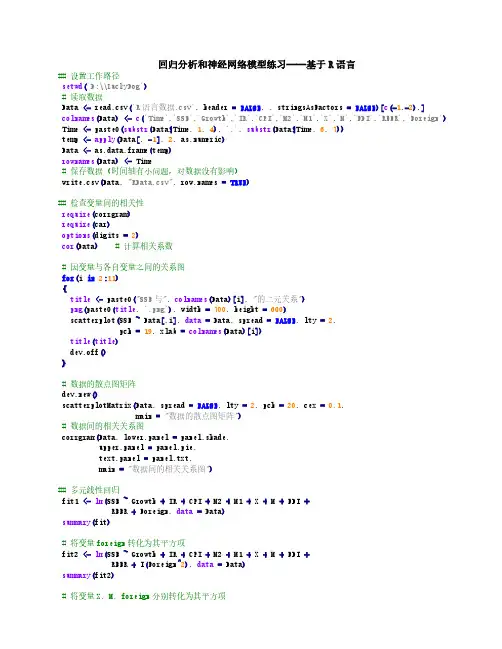
回归分析和神经网络模型练习——基于R语言##设置工作路径setwd('D:\\LuckyDog')#读取数据Data<-read.csv('R语言数据.csv',header=FALSE,,stringsAsFactors=FALSE)[c(-1,-2),] colnames(Data)<-c('Time','SSE','Growth','IR','CPI','M2','M1','X','M','FDI','REER','Foreign') Time<-paste0(substr(Data$Time,1,4),'.',substr(Data$Time,6,7))temp<-apply(Data[,-1],2,as.numeric)Data<-as.data.frame(temp)rownames(Data)<-Time#保存数据（时间轴有小问题，对数据没有影响）write.csv(Data,"RData.csv",s=TRUE)##检查变量间的相关性require(corrgram)require(car)options(digits=2)cor(Data)#计算相关系数#因变量与各自变量之间的关系图for(i in2:11){title<-paste0("SSE与",colnames(Data)[i],"的二元关系")png(paste0(title,'.png'),width=700,height=600)scatterplot(SSE~Data[,i],data=Data,spread=FALSE,lty=2,pch=19,xlab=colnames(Data)[i])title(title)dev.off()}#数据的散点图矩阵dev.new()scatterplotMatrix(Data,spread=FALSE,lty=2,pch=20,cex=0.1,main="数据的散点图矩阵")#数据间的相关关系图corrgram(Data,lower.panel=panel.shade,upper.panel=panel.pie,text.panel=panel.txt,main="数据间的相关关系图")##多元线性回归fit1<-lm(SSE~Growth+IR+CPI+M2+M1+X+M+FDI+REER+Foreign,data=Data)summary(fit)#将变量foreign转化为其平方项fit2<-lm(SSE~Growth+IR+CPI+M2+M1+X+M+FDI+REER+I(Foreign^2),data=Data)summary(fit2)#将变量X,M,foreign分别转化为其平方项fit3<-lm (SSE ~Growth +IR +CPI +M2+M1+I (X ^2)+I (M ^2)+FDI +REER +I (Foreign ^2),data =Data )summary (fit3)#将结果输出到outcome.doc#sink("outcome.doc",append =TRUE,split =TRUE)#summary(fit3)#AIC,BIC 准则判断三个模型拟合好坏（指标越小越好）AIC (fit1,fit2,fit3)BIC (fit1,fit2,fit3)#对fit3生成评价模型拟合情况的四幅图dev.new ()par (mfrow =c (2,2))plot (fit3)Call:lm(formula =SSE ~Growth +IR +CPI +M2+M1+I(X^2)+I(M^2)+FDI +REER +I(Foreign^2),data =Data)Residuals:Min 1Q Median 3Q Max -901.52195-315.18587-66.52143260.556221519.90405Coefficients:Estimate Std.Error t value Pr(>|t|)(Intercept)-10901.31459191461005271.5636725478871-2.067950.04158091*Growth 89.242872504368931.3448989843775 2.847130.00548969**IR -143.767694734867570.2548563880102-2.046370.04370374*CPI 93.949657629355245.7121742067872 2.055240.04281991*M2-77.252789604684833.2406560718311-2.324050.02242680*M140.062978773398513.7880195934089 2.905640.00463512**I(X^2)0.00020247133590.0001139036851 1.777570.07892986.I(M^2)-0.00044115559280.0001666573468-2.647080.00961917**FDI 8.9724175649034 2.7704019845048 3.238670.00169474**REER 34.41054967081669.7916449456622 3.514280.00069890***I(Foreign^2)-0.00000036862410.0000001059603-3.478890.00078512***---Signif.codes:0‘***’0.001‘**’0.01‘*’0.05‘.’0.1‘’1Residual standard error:490.3584on 88degrees of freedom Multiple R-squared:0.501946,Adjusted R-squared:0.4453489F-statistic:8.868766on 10and 88DF,p-value:0.0000000006470952df AIC fit1121537.337fit2121523.922fit3121519.926df BIC fit1121568.479fit2121555.064fit3121551.068#残差自相关检验durbinWatsonTest (fit3)#不相关#多重共线性检验(TURE 为可能存在多重共线问题)vif (fit3)>5##变量选择#向后回归require (MASS )stepAIC (fit3,direction ="backward")#结果显示经过变量变换后的fit3不需变量选择#全子集回归第一幅（左上）：若因变量与自变量线性相关，那残差值与拟合值就没有任何系统关联。

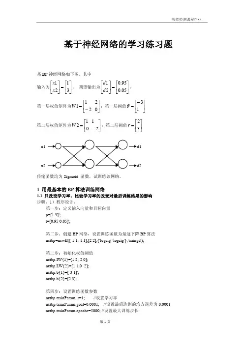
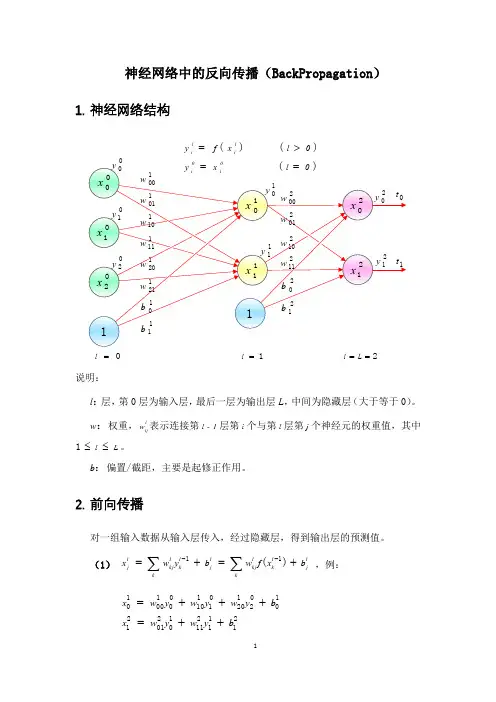
基于神经网络的学习练习题某BP 神经网络如下图。

其中输入为⎥⎦⎤⎢⎣⎡=⎥⎦⎤⎢⎣⎡3121x x ； 期望输出为⎥⎦⎤⎢⎣⎡=⎥⎦⎤⎢⎣⎡05.095.021d d ；第一层权值矩阵为⎢⎣⎡−=211W ⎥⎦⎤02；第一层阈值⎥⎦⎤⎢⎣⎡−=13θ 第二层权值矩阵为⎢⎣⎡=012W ⎥⎦⎤−21；第二层阈值⎥⎦⎤⎢⎣⎡=32r传输函数均为Sigmoid 函数，试训练该网络。

1 用最基本的BP 算法训练网络1.1 只改变学习率，比较学习率的改变对最后训练结果的影响 步骤：1）程序设计：第一步：定义输入向量和目标向量 p=[1 3]';t=[0.95 0.05]';第二步：创建BP 网络，设置训练函数为最速下降BP 算法 netbp=newff([-1 1;-1 1],[2 2],{'logsig' 'logsig'},'traingd');第三步：初始化权值阈值 netbp.IW{1}=[1 2;-2 0]; netbp.LW{2}=[1 1;0 -2]; netbp.b{1}=[-3 1]'; netbp.b{2}=[2 3]';第四步：设置训练函数参数netbp.trainParam.lr=1; //设置学习率netbp.trainParam.goal=0.0001; //设置最后达到的均方误差为0.0001 netbp.trainParam.epochs=5000; //设置最大训练步长d1d2第五步：训练神经网络 [netbp,tr]=train(netbp,p,t);程序运行的结果如下：经过346步运算达到设定的均方误差范围内。

最后输出⎥⎦⎤⎢⎣⎡=0.05140.9640Out训练后权值⎢⎣⎡= 1.5291-1.01071W ⎥⎦⎤1.41282.0322 ⎢⎣⎡= 1.4789-0.77132W ⎥⎦⎤2.9992-0.77392）分别改变学习率为1.5和0.5，观察结果 学习率5.1=α 5.0=α训练步长 263 786输出⎥⎦⎤⎢⎣⎡=0.05160.9640Out⎥⎦⎤⎢⎣⎡=0.05160.9640Out第一层权值 ⎢⎣⎡= 1.6030-1.01301W ⎥⎦⎤1.19092.0391⎢⎣⎡= 1.6078-1.01351W ⎥⎦⎤1.17662.0405第二层权值 ⎢⎣⎡= 1.4443-0.7744 2W ⎥⎦⎤3.1252-0.7806 ⎢⎣⎡= 1.4343-0.77512W ⎥⎦⎤3.1505-0.7816误差性能曲线结论1：学习率增大，所需的训练步长变短，即误差收敛速度快。

只需模仿即可。

就能轻松掌握。

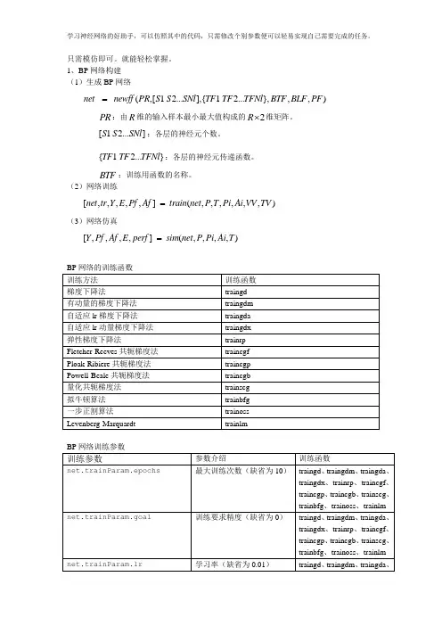
1、BP网络构建（1）生成BP网络net newff PR S S SNl TF TF TFNl BTF BLF PF=(,[1 2...],{ 1 2...},,,)R⨯维矩阵。

PR：由R维的输入样本最小最大值构成的2S S SNl：各层的神经元个数。

[1 2...]TF TF TFNl：各层的神经元传递函数。

{ 1 2...}BTF：训练用函数的名称。

（2）网络训练net tr Y E Pf Af train net P T Pi Ai VV TV=[,,,,,] (,,,,,,)（3）网络仿真=[,,,,] (,,,,)Y Pf Af E perf sim net P Pi Ai TBP网络的训练函数训练方法训练函数梯度下降法traingd有动量的梯度下降法traingdm自适应lr梯度下降法traingda自适应lr动量梯度下降法traingdx弹性梯度下降法trainrpFletcher-Reeves共轭梯度法traincgfPloak-Ribiere共轭梯度法traincgpPowell-Beale共轭梯度法traincgb量化共轭梯度法trainscg拟牛顿算法trainbfg一步正割算法trainossLevenberg-Marquardt trainlmBP网络训练参数训练参数参数介绍训练函数net.trainParam.epochs最大训练次数（缺省为10）traingd、traingdm、traingda、traingdx、trainrp、traincgf、traincgp、traincgb、trainscg、trainbfg、trainoss、trainlm net.trainParam.goal训练要求精度（缺省为0）traingd、traingdm、traingda、traingdx、trainrp、traincgf、traincgp、traincgb、trainscg、trainbfg、trainoss、trainlm net.trainParam.lr学习率（缺省为0.01）traingd、traingdm、traingda、traingdx、trainrp、traincgf、traincgp、traincgb、trainscg、trainbfg、trainoss、trainlm net.trainParam.max_fail 最大失败次数（缺省为5）traingd、traingdm、traingda、traingdx、trainrp、traincgf、traincgp、traincgb、trainscg、trainbfg、trainoss、trainlmnet.trainParam.min_grad 最小梯度要求（缺省为1e-10）traingd、traingdm、traingda、traingdx、trainrp、traincgf、traincgp、traincgb、trainscg、trainbfg、trainoss、trainlmnet.trainParam.show显示训练迭代过程（NaN表示不显示，缺省为25）traingd、traingdm、traingda、traingdx、trainrp、traincgf、traincgp、traincgb、trainscg、trainbfg、trainoss、trainlmnet.trainParam.time 最大训练时间（缺省为inf）traingd、traingdm、traingda、traingdx、trainrp、traincgf、traincgp、traincgb、trainscg、trainbfg、trainoss、trainlm net.trainParam.mc 动量因子（缺省0.9）traingdm、traingdxnet.trainParam.lr_inc 学习率lr增长比（缺省为1.05）traingda、traingdxnet.trainParam.lr_dec 学习率lr下降比（缺省为0.7）traingda、traingdxnet.trainParam.max_perf_inc 表现函数增加最大比（缺省为1.04）traingda、traingdxnet.trainParam.delt_inc 权值变化增加量（缺省为1.2）trainrpnet.trainParam.delt_dec 权值变化减小量（缺省为0.5）trainrpnet.trainParam.delt0 初始权值变化（缺省为0.07）trainrpnet.trainParam.deltamax 权值变化最大值（缺省为50.0）trainrpnet.trainParam.searchFcn 一维线性搜索方法（缺省为srchcha）traincgf、traincgp、traincgb、trainbfg、trainossnet.trainParam.sigma 因为二次求导对权值调整的影响参数（缺省值5.0e-5）trainscg mbda Hessian矩阵不确定性调节参数（缺省为5.0e-7）trainscg net.trainParam.men_reduc 控制计算机内存/速度的参量，内存较大设为1，否则设为2（缺省为1）trainlmnet.trainParam.mu μ的初始值（缺省为0.001）trainlm net.trainParam.mu_dec μ的减小率（缺省为0.1）trainlm net.trainParam.mu_inc μ的增长率（缺省为10）trainlmnet.trainParam.mu_maxμ的最大值（缺省为1e10） trainlm2、BP 网络举例 举例1、%traingd clear; clc;P=[-1 -1 2 2 4;0 5 0 5 7]; T=[-1 -1 1 1 -1];%利用minmax 函数求输入样本范围net = newff(minmax(P),[5,1],{'tansig','purelin'},'trainrp');net.trainParam.show=50;% net.trainParam.lr=0.05; net.trainParam.epochs=300; net.trainParam.goal=1e-5; [net,tr]=train(net,P,T);net.iw{1,1}%隐层权值 net.b{1}%隐层阈值net.lw{2,1}%输出层权值 net.b{2}%输出层阈值sim(net,P)举例2、利用三层BP 神经网络来完成非线性函数的逼近任务，其中隐层神经元个数为五个。

的记录是被我们所忽略的。
所有满足最小支持度3的1项频繁集如下 （其中巧克力、 香蕉、葡萄的支持度为1，不满足条件）
支持度
销售内容
3
4 4 5 7
冰淇淋
咖啡 果酱 牛奶 面包
所有满足最小支持度3的2项频繁集 如下 ：
支持度 3 销售内容 面包 咖啡 面包 冰淇淋 面包 牛奶 面包 果酱
递 归 执 行
的，比如在一个超市中会存在这样的概念 层次：蒙牛牌牛奶是牛奶，伊利牌牛奶是 牛奶，王子牌饼干是饼干，康师傅牌饼干 是饼干等。
• 可以用有向无环图 (directed acyclic graph ) 表示概念层次，如下：
从有向无环图 (directed acyclic graph )可以 看出—— 如果我们只是在数据基本层发掘关系， ｛蒙牛牌牛奶，王子牌饼干｝，｛蒙牛牌牛 奶，康师傅牌饼干｝，｛伊利牌牛奶，王子 牌饼干｝，｛伊利牌牛奶，康师傅牌饼干｝ 都不符合最小支持度。不过如果我们上升一 个层级，可能会发现｛牛奶，饼干｝ 的关 联规则是有一定支持度的。这样我们就可以 在较高的概念层次上发现关联规则。
w14 4 w46 6 5 w35
. . ..
w34
w56
. . .
3
图1 两层前馈神经网络
2
神经网络BP算法案例
• 首先算出单元4、5、6的输入、输出，具体结果见 表1，然后计算4、5、6的误差，见表2；NT中每条 有向加权边的新权重、每个隐藏层与输出层单元 的新偏置见表3。
图2 两层前馈神经网络
W35
0.2+0.9×(-0.0065)×1=0.194
0.1+0.9×0.1311=0.218 0.2+0.9×(-0.0065)=0.194

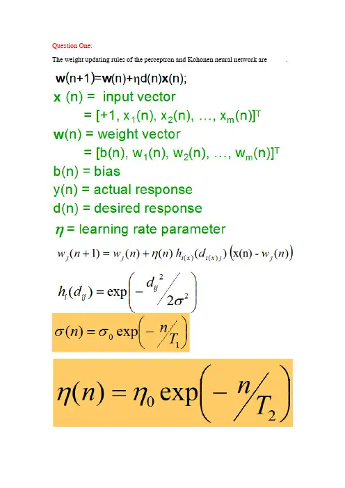
The weight updating rules of the perceptron and Kohonen neural network are _____.The limitation of the perceptron is that it can only model linearly separable classes. The decision boundary of RBF is__________linear______________________whereas the decision boundary of FFNN is __________________non-linear___________________________.Question Three:The activation function of the neuron of the Perceptron, BP network and RBF network are respectively________________; ________________; ______________.Question Four:Please present the idea, objective function of the BP neural networks (FFNN) and the learning rule of the neuron at the output layer of FFNN. You are encouraged to write down the process to produce the learning rule.Question Five:Please describe the similarity and difference between Hopfield NN and Boltzmann machine.相同：Both of them are single-layer inter-connection NNs.They both have symmetric weight matrix whose diagonal elements are zeroes.不同：The number of the neurons of Hopfield NN is the same as the number of the dimension (K) of the vector data. On the other hand, Boltzmann machine will have K+L neurons. There are L hidden neuronsBoltzmann machine has K neurons that serves as both input neurons and output neurons (Auto-association Boltzmann machine).Question Six:Please explain the terms in the above equation in detail. Please describe the weight updating equations of each node in the following FFNN using the BP learning algorithm. (PPT原题y=φ(net)= φ(w0+w1x1+w2x2))W0=w0+W1=w1+W2=w2+Question Seven:Please try your best to present the characteristics of RBF NN.(1)RBF networks have one single hidden layer.(2)In RBF the neuron model of the hidden neurons is different from the one of the output nodes.(3)The hidden layer of RBF is non-linear, the output layer of RBF is linear.(4)The argument of activation function of each hidden neuron in a RBF NN computes the Euclidean distance between input vector and the center of that unit.(5)RBF NN uses Gaussian functions to construct local approximations to non-linear I/O mapping.Question Eight:Generally, the weight vectors of all neurons of SOM is adjusted in terms of the following rule:w j(n+1)=w j(n)+η(n)h i(x)(d i(x)j)(x(n)-w j(n)).Please explain each term in the above formula.: weight value of the j-th neuron at iteration n: neighborhood functiondji: lateral distance of neurons i and j: the learning rate: the winning neuron most adjacent to XX: one input example。

5. 链式法则
如果函数 u (t )及 v (t )都在 t 点可导，复合函数 z f(u,v)在对应点(u,v)具 有连续偏导数，z 在对应 t 点可导，则其导数可用下列公式计算：
dz z du z dv dt u dt v dt
6. 神经元误差
定义 l 层的第 i 个神经元上的误差为 il 即： （7）
5
附：激活函数
非线性： 当激活函数是线性的时候，一个两层的神经网络就可以逼近基 本上所有的函数了。但是，如果激活函数是恒等激活函数的时候（即 f(x)=x） ，就不满足这个性质了，而且如果 MLP 使用的是恒等激活函数， 那么其实整个网络跟单层神经网络是等价的。 可微性： 当优化方法是基于梯度的时候，这个性质是必须的。 单调性： 当激活函数是单调的时候，单层网络能够保证是凸函数。 f(x)≈x： 当激活函数满足这个性质的时候， 如果参数的初始化是 random 的很小的值， 那么神经网络的训练将会很高效； 如果不满足这个性质， 那 么就需要很用心的去设置初始值。 输出值的范围： 当激活函数输出值是 有限 的时候，基于梯度的优化方 法会更加 稳定，因为特征的表示受有限权值的影响更显著；当激活函数 的输出是 无限 的时候， 模型的训练会更加高效， 不过在这种情况小， 一 般需要更小的 learning rate.
l i

j
l 1 E x j x lj 1 xil

j
x lj 1 x
l i
jl 1 ，其中 l L
将公式（1） x j
l 1

w
k
l 1 l kj k
y blj 1
w
k
l 1 kj
f( xkl ) blj 1 ，对 x i 的求导

2022/3/23
BP神经网络求解异或问题的权值调整
输入样本（1，1，0）时，求解各对应参数：
各神经元的输出
hi1(0) x1(0)w11(0) x2(0)w21(0) 1 0.5 1 0.5 1 hi2(0) x2(0)w12(0) x2(0)w22(0) 1
X1(k) X2(k)
输入层
隐含层
q
wiNh+1
=
w
N ih
+
h(Biblioteka do(k) who)f (hih(k)) xi(k)
o=1
输出层
ho1(0)
f
(hi1
)
1
1 e1
0.731
ho2(0)
f
(hi2
)
1
1 e1
0.731
yi(0) ho1(0)w1y (0) ho2(0)w2y (0) 0.731 0.5 0.731 0.5 0.731
0.015
h2(0) o (0)w2y (0)ho2(0)(1 ho2(0)) 0.015 w11(0) h1(0)x1(0) 0.5 0.0151 0.007 w21(0) h1(0)x2(0) 0.5 0.015 1 0.007
X1(k) X2(k)
n
hih (k) wih xi (k) bh
i1
hoh (k) f(hih (k))
w11 1
w12
w21
2
w22
1
w1y1
w2y1
p
yio (k ) whohoh (k ) bo h1
y1 yoo(k) f( yio(k))
2
whNo1 whNo (do (k ) yoo (k )) yoo (k )hoh (k )

模式识别复习题1.BP 神经网络是由哪三层构成的前馈网络？答：输入层、隐含层、输出层。

2 .BP 神经网络的基本特点有哪些？答：BP 网络具有以下主要优点：(1)只有有足够多的隐含层节点和隐含层，BP 网络才可以逼近任意的非线性映射关系。

(2)BP 网络的学习算法属于局部逼近的方法，因此它具有较好的泛化能力。

(3)BP 网络具有很好的逼近非线性映射的能力。

BP 网络的主要缺点如下：(1)收敛速度慢。

(2)容易陷入局部极值点。

(3)难以确定隐含层和隐含层节点的个数。

3 .Hebb 的学习规则是什么？答：如果神经网络中某一神经元与另一直接与其相连的神经元同时处于兴奋状态,那么这两个神经元之间的连接强度应该加强。

4 .人工神经元模型中的非线性作用函数f,常用的三种非线性输出函数有哪些？5 .神经网络按照信息的流向可以分为哪两大类神经网络？答：前馈神经网络和反馈神经网络。

6 .在什么前提情况下，最小风险贝叶斯决策等价于最小错误率贝叶斯决策，或者说最小错误率贝叶斯决策是最小风险贝叶斯决策的特例。

答：最小错误率贝叶斯决策就是在采用07损失函数条件下的最小风险贝叶斯决策，即前者是后者的特例。

7 .贝叶斯公式中是哪三者之间的关系？答：先验概率P(31);后验概率P(3∣∣X);条件概率P(X ∣3j° 8 .模式识别的一般步骤有哪些？答：数据采集(数据获取)T 数据预处理T 特征提取与特征选择T 分类判别(决策分析)。

9 .假定在细胞识别中，病变细胞的先验概率和正常细胞的先验概率分别为P(ω1)=0.05,P(ω2)=0.95o 现有一待识别细胞，其观察值为X,从类条件概率密度发布曲线上查得：P(X ∣3,=0.5,P(X ∣ω2)=0.2o 试对细胞X 进行分类。

解：［方法1］：通过后验概率计算。

z1、P(X∣ω1)P(ω1) 0.5x0.05P(ω1X)=-^― ------------------ -------- = ------------------------------- ≈0.16∑÷s ,1P(XQi)PQD0.05×0.5+0.95×0.20.2×0.950.05×0.5+0.95×0.2∙.'P(ω2∣X)>P(ω1∣X)ΛX ∈ω2P(ω2∣X) =≈ 0. 884［方法二］:利用先验概率和类概率密度计算。

double D[100];
//初始化样本
void init_XD(void)
{
for (int i=0;i<100;i++)
{X[i]=-2*pi+i*0.04*pi;
D[i]=fabs(cos(X[i]));
}
}
//激励函数f(N)
double f(double N)
{
return 1/(1+exp(-N));
}
W2[m][n]=W2[m][n]+u*D2[m][n];
}
}
//对于输入层
for (int a=0;a<3;a++)
{
for (int b=0;b<4;b++)
{
for (int c=0;c<5;c++)
{
D1[a]=(sample_d-output_y)*diff_f(N4)*W4[c]*diff_f(N3[c])*W3[c][b]*diff_f(N2[b])*W2[b][a]*diff_f(N1[a])*sample_x;
}
}
W1[a]=W1[a]+u*D1[a];
}
}
int main()
{
init_XD();
double p=0;
ofstream file1("c:\\a.txt");
for(int j=0;j<100;j++)
{
file1<<X[j]<<" ";
}
file1<<endl;
for (int k=0;k<100;k++)

BP神经⽹络maab实例简单⽽经典p=p1';t=t1';[pn,minp,maxp,tn,mint,maxt]=premnmx(p,t); %原始数据归⼀化net=newff(minmax(pn),[5,1],{'tansig','purelin'},'traingdx'); %设置⽹络,建⽴相应的BP⽹络% 训练⽹络,pn,tn); %调⽤TRAINGDM算法训练BP⽹络pnew=pnew1';pnewn=tramnmx(pnew,minp,maxp);anewn=sim(net,pnewn); %对BP⽹络进⾏仿真anew=postmnmx(anewn,mint,maxt); %还原数据y=anew';1、BP⽹络构建（1）⽣成BP⽹络PR：由R维的输⼊样本最⼩最⼤值构成的2R 维矩阵。

[ 1 2...]S S SNl：各层的神经元个数。

TF TF TFNl：各层的神经元传递函数。

{ 1 2...}BTF：训练⽤函数的名称。

（2）⽹络训练（3）⽹络仿真{'tansig','purelin'},'trainrp'BP⽹络的训练函数BP⽹络训练参数2、BP⽹络举例举例1、%traingd clear;clc;P=[-1 -1 2 2 4;0 5 0 5 7];T=[-1 -1 1 1 -1];%利⽤minmax函数求输⼊样本范围net = newff(minmax(P),T,[5,1],{'tansig','purelin'},'trainrp');隐层权值{1}%隐层阈值{2,1}%输出层权值{2}%输出层阈值sim(net,P)举例2、利⽤三层BP神经⽹络来完成⾮线性函数的逼近任务，其中隐层神经元个数为五个。

样本数据：解：-，所以利⽤双极性Sigmoid函数作为转移函数。

44
BP网络应用实例
x=imread(m,’bmp’); bw=im2bw(x,0.5); 为二值图像 [i,j]=find(bw==0); ）的行号和列号 imin=min(i)； ）的最小行号 imax=max(i); ）的最大行号 ％读人训练样本图像丈件 ％将读人的训练样本图像转换 ％寻找二值图像中像素值为0(黑
4
BP网络学习算法
图5．5具有多个极小点的误差曲面
5
BP网络学习算法
另外一种情况是学习过程发生振荡，如图5．6所示 。 误差曲线在m点和n点的梯度大小相同，但方向相反 ，如果第k次学习使误差落在m点，而第k十1次学习 又恰好使误差落在n点。 那么按式（5．2）进行的权值和阈值调整，将在m 点和n点重复进行，从而形成振荡。
图 5.16
待分类模式
20
BP网络应用实例
解（1）问题分析 据图5．16所示两类模式可以看出，分类为简单的非 线性分类。有1个输入向量，包含2个输入元素；两 类模式，1个输出元素即可表示；可以以图5．17所 示两层BP网络来实现分类。
图 5.17
两层BP网络
21
BP网络应用实例
（2）构造训练样本集
6
BP网络学习算法
图5．6学习过程出现振荡的情况
7
BP网络的基本设计方法
BP网络的设计主要包括输人层、隐层、输出层及各 层之间的传输函数几个方面。 1．网络层数 大多数通用的神经网络都预先确定了网络的层数，而 BP网络可以包含不同的隐层。
8
BP网络的基本设计方法
但理论上已经证明，在不限制隐层节点数的情况下 ，两层（只有一个隐层）的BP网络可以实现任意非 线性映射。 在模式样本相对较少的情况下，较少的隐层节点， 可以实现模式样本空间的超平面划分，此时，选择 两层BP网络就可以了；当模式样本数很多时，减小 网络规模，增加一个隐层是必要的，但BP网络隐层 数一般不超过两层。

bp算法的案例BP算法（Back Propagation）是一种常见的神经网络训练算法，用于解决分类、回归等问题。

下面是一个关于使用BP算法进行手写数字识别的案例，包括神经网络结构、数据预处理、模型训练和模型评估等方面的内容。

1. 神经网络结构手写数字识别是一个多类别分类问题，常用的神经网络结构是多层感知器（Multi-Layer Perceptron，MLP）。

MLP通常包含输入层、若干隐藏层和输出层。

输入层接收手写数字的像素值作为输入，每个像素点对应一个输入节点。

隐藏层是一些全连接层，每一层都由若干个神经元组成，可以通过增加隐藏层的数量和神经元的数量来增加网络的复杂度。

输出层是一个全连接层，每个输出节点对应一个类别，其中概率最大的节点对应的类别即为预测结果。

2. 数据预处理手写数字识别通常使用MNIST数据集，该数据集包含了60000个用于训练的样本和10000个用于测试的样本。

每个样本是一张28x28像素的黑白图片，表示一个手写数字。

为了进行神经网络的训练，需要将图片数据转化为合适的格式，通常是将像素值进行标准化，将灰度值除以255，使其范围在0到1之间。

同时，还需要将每个样本的标签进行独热编码（One-Hot Encoding），将其转化为一个向量，其中目标类别对应的位置为1，其余位置为0。

3. 模型训练在进行模型训练之前，需要对神经网络的超参数进行设置，如学习率、隐藏层数量、每层的神经元数量等。

通过调节这些超参数可以影响模型的性能。

然后，使用训练数据集对神经网络进行训练。

训练过程中，首先将标准化后的像素值输入到网络中，通过前向传播计算出每个节点的输出值，然后根据实际的标签值和预测的输出值计算损失函数（常用的损失函数有均方误差和交叉熵损失）。

接下来，使用反向传播算法（Back Propagation）计算出每个节点的梯度，然后根据梯度更新网络中的参数，以减小损失函数的值。

反复迭代这一过程，直到模型收敛或者达到设定的迭代次数。

一 简述人工神经网络常用的网络结构和学习方法。

（10分）答：1、人工神经网络常用的网络结构有三种分别是：BP 神经网络、RBF 神经网络、Kohonen 神经网络、ART 神经网络以及Hopfield 神经网络。

人工神经网络模型可以按照网络连接的拓扑结构分类，还可以按照内部信息流向分类。

按照拓扑结构分类：层次型结构和互连型结构。

层次型结构又可分类：单纯型层次网络结构、输入层与输出层之间有连接的层次网络结构和层内有互联的层次网络结构。

互连型结构又可分类：全互联型、局部互联型和稀疏连接性。

按照网络信息流向分类：前馈型网络和反馈型网络。

2、学习方法分类：⑴.Hebb 学习规则：纯前馈网络、无导师学习。

权值初始化为0。

⑵.Perceptron 学习规则：感知器学习规则，它的学习信号等于神经元期望输出与实际输出的差。

单层计算单元的神经网络结构，只适用于二进制神经元。

有导师学习。

⑶.δ学习规则：连续感知学习规则，只适用于有师学习中定义的连续转移函数。

δ规则是由输出值与期望值的最小平方误差条件推导出的。

⑷.LMS 学习规则：最小均放规则。

它是δ学习规则的一个特殊情况。

学习规则与神经元采用的转移函数无关的有师学习。

学习速度较快精度较高。

⑸.Correlation 学习规则：相关学习规则，他是Hebb 学习规则的一种特殊情况，但是相关学习规则是有师学习。

权值初始化为0。

⑹.Winner-Take-All 学习规则：竞争学习规则用于有师学习中定义的连续转移函数。

权值初始化为任意值并进行归一处理。

⑺.Outstar 学习规则：只适用于有师学习中定义的连续转移函数。

权值初始化为0。

2．试推导三层前馈网络BP 算法权值修改公式，并用BP 算法学习如下函数：21212221213532)(x x x x x x x x f -+-+=,其中：551≤≤-x ，552≤≤-x 。

基本步骤如下：（1）在输入空间]5,5[1-∈x 、]5,5[2-∈x 上按照均匀分布选取N 个点（自行定义），计算)(21x x f ,的实际值，并由此组成网络的样本集；（2）构造多层前向网络结构，用BP 算法和样本集训练网络，使网络误差小于某个很小的正数ε；（3）在输入空间上随机选取M 个点（N M >，最好为非样本点），用学习后的网络计算这些点的实际输出值，并与这些点的理想输出值比较，绘制误差曲面；（4）说明不同的N 、ε值对网络学习效果的影响。

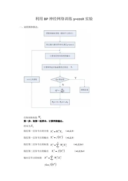
BP神经网络及其MATLAB实例问题：BP神经网络预测2020年某地区客运量和货运量公路运量主要包括公路客运量和公路货运量两方面。

某个地区的公路运量主要与该地区的人数、机动车数量和公路面积有关，已知该地区20年(1999-2018)的公路运量相关数据如下：人数/万人：20.5522.4425.3727.1329.4530.1030.9634.0636.4238.09 39.1339.9941.9344.5947.3052.8955.7356.7659.1760.63机动车数量/万辆：0.60.750.850.9 1.05 1.35 1.45 1.6 1.7 1.85 2.15 2.2 2.25 2.35 2.5 2.6 2.7 2.85 2.95 3.1公路面积/单位：万平方公里：0.090.110.110.140.200.230.230.320.320.34 0.360.360.380.490.560.590.590.670.690.79公路客运量/万人：5126621777309145104601138712353157501830419836 21024194902043322598251073344236836405484292743462公路货运量/万吨：1237137913851399166317141834432281328936 11099112031052411115133201676218673207242080321804影响公路客运量和公路货运量主要的三个因素是：该地区的人数、机动车数量和公路面积。

Matlab代码实现%人数(单位：万人)numberOfPeople=[20.5522.4425.3727.1329.4530.1030.9634.0636.42 38.0939.1339.9941.9344.5947.3052.8955.7356.7659.1760.63];%机动车数(单位：万辆)numberOfAutomobile=[0.60.750.850.91.051.351.451.61.71.852.15 2.2 2.25 2.35 2.5 2.6 2.7 2.85 2.95 3.1];%公路面积(单位：万平方公里)roadArea=[0.090.110.110.140.200.230.230.320.320.340.360.360.380.490.560.590.590.670.690.79];%公路客运量(单位：万人)passengerVolume=[5126621777309145104601138712353157501830419836 21024194902043322598251073344236836405484292743462];%公路货运量(单位：万吨)freightVolume=[123713791385139916631714183443228132893611099 112031052411115133201676218673207242080321804];%输入数据矩阵p=[numberOfPeople;numberOfAutomobile;roadArea];%目标（输出）数据矩阵t=[passengerVolume;freightVolume];%对训练集中的输入数据矩阵和目标数据矩阵进行归一化处理[pn,inputStr]=mapminmax(p);[tn,outputStr]=mapminmax(t);%建立BP神经网络net=newff(pn,tn,[372],{'purelin','logsig','purelin'});%每10轮回显示一次结果net.trainParam.show=10;%最大训练次数net.trainParam.epochs=5000;%网络的学习速率net.trainParam.lr=0.05;%训练网络所要达到的目标误差net.trainParam.goal=0.65*10^(-3);%网络误差如果连续6次迭代都没变化，则matlab会默认终止训练。

▪
26、要使整个人生都过得舒适、愉快，这是不可能的，因为人类必须具备一种能应付逆境的态度。——卢梭
▪
27、只有把抱怨环境的心情，化为上进的力量，才是成功的保证。——罗曼·罗兰
▪
28、知之者不如好之者，好之者不如乐之者。——孔子
神经网络BP网络 数学建模
31、别人笑我太疯癫，我笑他人看不 穿。(名 言网) 32、我不想听失意者的哭泣，抱怨者 的牢骚 ，这是 羊群中 的瘟疫 ，我不 能被它 传染。 我要尽 量避免 绝望， 辛勤耕 耘，忍 受苦楚 。我一 试再试 ，争取 每天的 成功， 避免以 失败收 常在别 人停滞 不前时 ，我继 续拼搏 。
▪
29、勇猛、大胆和坚定的决心能够抵得上武器的精良。——达·芬奇
▪
30、意志是一个强壮的盲人，倚靠在明眼的跛子肩上。——叔本华
谢谢！Biblioteka 5333、如果惧怕前面跌宕的山岩，生命 就永远 只能是 死水一 潭。 34、当你眼泪忍不住要流出来的时候 ，睁大 眼睛， 千万别 眨眼!你会看到 世界由 清晰变 模糊的 全过程 ，心会 在你泪 水落下 的那一 刻变得 清澈明 晰。盐 。注定 要融化 的，也 许是用 眼泪的 方式。
35、不要以为自己成功一次就可以了 ，也不 要以为 过去的 光荣可 以被永 远肯定 。