crystal-ball-基础教程

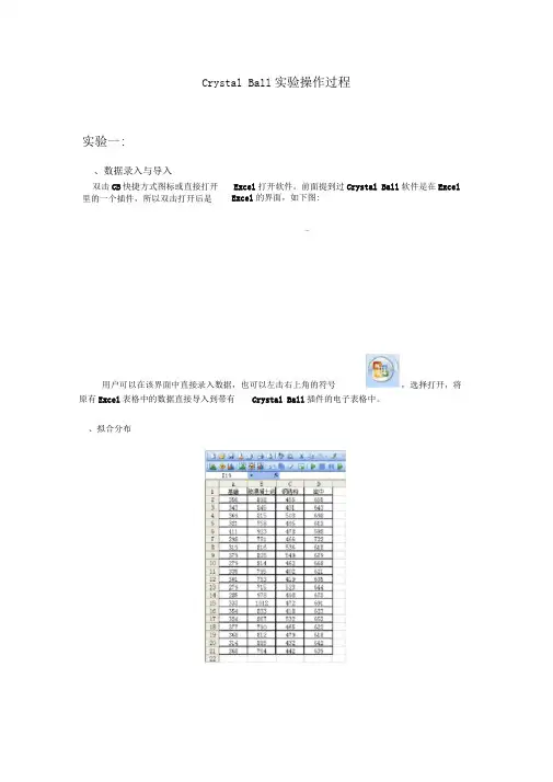
C r y s t a l B a l l实验操作过程Crystal Ball实验操作过程实验一：一、数据录入与导入双击CB快捷方式图标或直接打开Excel打开软件。

前面提到过Crystal Ball 软件是在Excel里的一个插件，所以双击打开后是Excel的界面，如下图：图 1用户可以在该界面中直接录入数据，也可以左击右上角的符号，选择打开，将原有Excel表格中的数据直接导入到带有Crystal Ball插件的电子表格中。

二、拟合分布图2(1)对数据进行标准化处理(减少原数据相互间的距离对拟合分布的影响)通过Average计算每个分布工程样本数据的均值,然后各个样本数据除以相应的均值,对数据进行标准化处理。

（2）拟合分布选取表格区域，点击工具栏上“Run-Tools-Batch Fit”,如图3所示。

图3在操作对话框中，选择“next”,至图4对话框对相应命令进行选择,可得到拟合过程的相关数据。

图4注：对于卡方检验，水晶球软件计算p值，p值大于0.5一般表示紧密拟合；对于科尔莫格洛夫-斯米尔诺夫检验，一般地，小于0.03的K-S值表明良好拟合；对于安德森-达林检验，小于1.5的计算值一般表明拟合优良。

实验二:一.按照实验一的操作,先将数据在Crystal Ball软件打开.二、假设单元格概率分布的定义及相关操作输入数据后，进行随机变量假设单元格概率分布的定义。

这里假设使用悲观时间的单元格来进行概率分布的定义。

（注：对于假设单元格的选择，并无太多的限制，因为定义各种概率的分布，是由相应的参数确定的，因此选择的假设单元格不同对结果并没有影响。

）有一点需要注意的是，选择假设单元格时，该单元格应当是一确定的数字，而不能是公式.选定单元格（如单元格I2）后，点击工具栏上的，随即弹出图5，CB 软件中提供22种不同的分布可供选择，根据实验任务书的要求，第一和第二项分部分项工程服从三参数beta分布，因此，选择BtaPERT分布，并填入相应参数，即可完成对“基坑支护挖土方”的定义，如图6所示。

Crystal Ball实验操作过程实验一:、数据录入与导入双击CB快捷方式图标或直接打开Excel打开软件。

前面提到过Crystal Ball软件是在Excel 里的一个插件，所以双击打开后是Excel的界面，如下图:»nm用户可以在该界面中直接录入数据，也可以左击右上角的符号，选择打开，将原有Excel表格中的数据直接导入到带有Crystal Ball插件的电子表格中。

、拟合分布(1)对数据进行标准化处理(减少原数据相互间的距离对拟合分布的影响)通过Average计算每个分布工程样本数据的均值，然后各个样本数据除以相应的均值对数据进行标准化处理。

(2)拟合分布选取表格区域，点击工具栏上“ Run-Tools-Batch Fit ”，如图3所示图3在操作对话框中，选择next”至图4对话框对相应命令进行选择，可得到拟合过程的相关数据注：对于卡方检验，水晶球软件计算p值，p值大于0.5 —般表示紧密拟合；对于科尔莫格洛夫-斯米尔诺夫检验，一般地，小于0.03的K-S值表明良好拟合;对于安德森-达林检验，小于1.5的计算值一般表明拟合优良。

实验二:•按照实验一的操作，先将数据在Crystal Ball软件打开.、假设单元格概率分布的定义及相关操作输入数据后，进行随机变量假设单元格概率分布的定义。

这里假设使用悲观时间的单元格来进行概率分布的定义。

（注：对于假设单元格的选择，并无太多的限制，因为定义各种概率的分布，是由相应的参数确定的，因此选择的假设单元格不同对结果并没有影响。

）有一点需要注意的是，选择假设单元格时，该单元格应当是一确定的数字，而不能是公式•选定单元格（如单元格12）后，点击工具栏上的二工，随即弹出图5，CB软件中提供22种不同的分布可供选择，根据实验任务书的要求，第一和第二项分部分项工程服从三参数beta分布，因此，选择BtaPERT分布，并填入相应参数，即可完成对“基坑支护挖土方”的定义，如图6所示。

风险管理软件CrystalBall操作指南Monte-Carlo Simulation with Crystal Ball®To run a simulation using Crystal Ball®:1. Setup SpreadsheetBuild a spreadsheet that will calculate the performance measure (e.g., profit) in terms of the inputs (random or not). For random inputs, just enter any number.2. Define Assumptions—i.e., random variablesDefine which cells are random, and what distribution they should follow.3. Define Forecast—i.e., output or performance measureDefine which cell(s) you are interested in forecasting (typically the performance measure, e.g., profit).4. Choose Number of TrialsSelect the number of trials. If you would later like to generate the Sensitivity Analysis chart, choose 〝Sensitivity Analysis〞under Options in Run Preferences.5. Run SimulationRun the simulation. If you would like to change parameters and re-run the simulation, you should 〝reset〞 the simulation (click on the 〝Reset Simulation〞 button on the toolbar or in the Run menu) first.6. View ResultsThe forecast window showing the results of the simulation appears automatically after (orduring) the simulation. Many different results are available (frequency chart, cumulative chart, statistics, percentiles, sensitivity analysis, and trend chart). The results can be copied into the worksheet.Crystal Ball Toolbar:Define Define Run Start Reset Forecast Trend Assumptions Forecast Preferences Simulation Simulation Window ChartRecall the Walton Bookstore example: It is August, and they must decide how many of next year’s nature calendars to order. Each calendar costs the bookstore $7.50 and is sold for $10. After February, all unsold calendars are returned to the publisher for a refund of $2.50 per calendar. Suppose Walton predicts demand will be somewhere between 100 and 300 (discrete uniform).Demand = d ~ Uniform[100, 300]Order Quantity = Q (decision variable)Revenue = $10 * Min(Q, d)Cost = $7.50 * QRefund = $2.50 * Max(Q–d, 0)Profit = Revenue – Cost + RefundStep #1 (Setup Spreadsheet)Step #2 (Define Assumptions —i.e., random variables)—color code (blue):and click on the 〝Define Assumptions 〞 button in toolbar (or in the Cell menu):Select type of distribution:Provide parameters of distributions:Walton Bookstore Simulation with Crystal Ball®Step #3 (Define Forecast—i.e., output)click on the 〝Define Forecast〞 button in toolbar (or in the Cell menu),and fill in the Define Forecast dialogue box.Step #4 (Choose Number of Trials)Click on the 〝Run Preferences〞 button in toolbar (or in the Run menu):and select the number of trials to run.Walton Bookstore Simulation with Crystal Ball®Step #5 (Run Simulation)Click on the 〝Start Simulation〞 button in toolbar (or Run in the Run menu):Step #6 (View Results)The results of the simulation can be viewed in a variety of different ways (frequency chart, cumulative chart, statistics, and percentiles). Choose different options under the View menuin the forecast window.The results can be copied into a worksheet or Word document (choose Copy under the Edit menu in the simulation output window.Using Trend Charts to Find the Impact of Order Quantityon Potential ProfitDefine several forecast cells (G14:G18) for several possible order quantities (Q=100, 150, 200, 250, 300). Use the same random order quantity for each to compare them more equally (i.e., one assumption cell for demand—C14—with the rest set equal to C14).After running the simulation, choose 〝Open Trend Chart〞 in the Run menu. This chart gives 〝certainty bands〞 for the forecast cells. 10% of the time, the project duration will fall within the inner band (light blue), 25% of the time within the 2nd band (red), 50% of the time within the third band (green), and 90% of the time within the outside band (dark blue).Project Management—Global OilGlobal Oil is planning to move their credit card operation to Des Moines, Iowa from their home office in Dallas. The move involves many different divisions within the company. Real estate must select one of three available office sites. Personnel has to determine which employees from Dallas will move, how many new employees to hire, and who will train them. The systems group and treasurer’s office must organize the new operating procedure and make financial arrangements. The architects will have to design the interior space, and oversee needed structural improvements. Each site is an existing building with sufficient open space, but office partitions, computer facilities, furnishings, and so on, must all be provided.A complicating factor is that there is an interdependence of activities. In other words, some parts of the project cannot be started until other parts are completed. For example, Global cannot construct the interior of an office before it has been designed. Neither can it hire new employees until it has determined its personnel requirements.The necessary activities and their necessary predecessors (due to interdependence) are listed below. Three estimates are made for the completion time of each activity—the minimum time, most likely time, and maximum time.Start EndGlobal Oil Simulation with Crystal Ball®Step #1 (Setup Spreadsheet)Step #2 (Define Assumptions—i.e., random variables)Each of the random activity times (B, C, D, E, G, and I) is assumed to follow the triangular distribution.Global Oil Simulation with Crystal Ball®Step #3 (Define Forecast—i.e., output)Cell J15 is the forecast cell:Step #4 (Choose Number of Trials)500 trials were run. In addition, Sensitivity Analysis was enabled in the Options of the Run Preferences dialogue box. This allows for the generation of sensitivity analysis results later.Step #5 (Run Simulation)Step #6 (View Results)Additional Results Available with Crystal Ball®Slide the triangles below the histograms to determine the probability that the output (project duration) is less than a certain value (e.g., a deadline), greater than a certain value, or between any two values (by sliding both triangles).Alternatively, you can type in values for the lower bound or upper bound to determine the probability. You can also type in a probability (in 〝Certainty〞), and it will determine the range that has that probability.There is a 79% chance the project will be completed within 150 days.There is a 2.4% chance that the project will take more than 160 days.Sensitivity ChartChoose 〝Open Sensitivity Chart〞 in the Run menu. Note that this chart is only available ifyou selected the 〝Sensitivity Analysis〞 option under Run Preferences. This chart gives an indication as to which random variables (activity times) have the greatest impact on the output cell (project completion time).Variability in activity E has the greatest impact on overall project duration, followed by activity D, C, I, and B. Variability in activity G has almost no impact.Fitting a DistributionCrystal Ball can be used to 〝fit〞 a distribution to data.The following data has been collected for the previous 100 phone calls to a mail-order house:(80 rows have been hidden)Fitting Data to a DistributionUsing Crystal Ball® to fit data to a distribution1. Select a spreadsheet cell.2. Choose Define Assumption.3. Click the Fit button, then select the source of the fitted data.4. Click the Next button, then select the distributions to try to fit.5. Click OK.Interarrival TimeService Time。

水晶球软件2000专业版(Crystal Ball®2000 Professional Edition)初级教程摘要加载在微软公司(Microsoft®)的电子表格软件(Excel®)上的水晶球软件2000专业版(Crystal Ball®2000 Professional Edition)是一个易于使用的软件它可以帮助你分析与你的电子表格模型相关的风险和不确定性这个软件包括蒙特卡洛模拟水晶球时间序列预测水晶球预言家最优选择优化查询和用来构造定制界面和程序的开发工具箱由于电子表格缺乏设计和分析可选方案的能力所以仅用电子表格来估算一个事件发生的概率是不合适的而加载了水晶球软件的电子表格模型就能具备这样的功能从而帮助用户洞察模型运行和结果产生的机制本初级教程通过一个媒体产业的实例来演示蒙特卡洛模拟和时间序列预测工具如何用于一个电子表格模型为商业决策的内在风险提供更深入的了解和度量1 序言1.1 电子表格模型和风险分析风险就是不确定性是指发生损失危害和其它不愉快事件的可能性大多数人偏好低风险期待成功收益或其它形式获利的较高概率举例来说如果下个月的销售超过一定数额一种令人愉快的事件那么这些订单会使存货减少从而导致商品运送的延迟一种令人不愉快的事件反过来商品运送的延迟则会导致订单的流失发生这种情况的可能性就代表了一种风险当使用电子表格模型时分析家习惯将那些本来不确定的变量用其平均值或其最佳估计值来输入这是因为电子表格软件只允许他们在一个单元格内输入一个数值或一个公式这些确定的模型只能产生一个结果而模型结果将被用作商业或技术决策的根据为了把握模型中本身存在的那些不确定性分析家只能通过手工方式来改变模型变量分析它们对关键结果的影响来简单地实现方案分析这种方法提供了可能结果的一定范围但它无法使人得知那些特定结果出现的可能性管理者经常需要知道那些不确定变量分别取什么值的时候方案会达到一个最佳情况或在什么时候方案会达到一个最差情况又在什么时候方案又会达到一个最可能情况那些包含不确定性因素的实际问题绝大部分都是很复杂的为了计算每一种可能发生的结果就需要将所有输入变量的各种可选数值进行组合对于复杂的实际问题这种组合的数量是非常庞大的很难一一实现因此在实际问题中这种办法很难奏效1.2 蒙特卡洛模拟为了解决电子表格模型在风险分析方面存在的局限性蒙特卡洛模拟是一个现成的办法由于电子表格软件本身不具有模拟运行和模拟分析的能力所以用户必须依靠象水晶球软件这样一些加载在电子表格软件上的第三方程序来扩充电子表格软件的功能针对电子表格软件水晶球软件增加了两项功能一是用概率分布来替代单个数值二是可以进行模型的随机模拟通过水晶球软件可以生成量化的基于概率的电子表格模型例如可以得到以75%的概率保证在预算内或某一水库装满一亿桶油的可能性有90%这样的结果蒙特卡洛模拟是一项已被确认正确并且行之有效的技术它只要求计算机具有一个随机数表或一个随机数生成器我们可以通过数学方法来产生服从某一概率分布的随机数蒙特卡洛模拟是用一个城市的名字来命名的这个城市就是摩纳哥的蒙特卡洛它以充满各种冒险游戏的赌场而闻名常见的赌博游戏有轮盘赌投掷骰子老虎机等在蒙特卡洛模拟中为了模拟一个模型需要随机选择变量的取值这与赌博中的随机现象很相似当你投掷一个骰子时你知道会出现12345或6中的某一点但你不知道具体某一次投掷时会出现哪一个点与投掷骰子相同随机变量例如利率需求量股价存货量每分钟电话呼叫次数的取值范围是确定的但在具体某一时间或某一事件时取到的值是不确定的模拟可以产生大量的方案通过分析这些方案可以深入了解电子表格模型中蕴涵的风险和机理只要使用得当蒙特卡洛模拟就能展现非常有价值的视角而这是确定性模型所得不到的2 水晶球软件2000专业版水晶球软件2000专业版是一个办公软件套件以基于电子表格的分析工具为特色包括蒙特卡洛模拟水晶球时间序列预测水晶球预言家和最优选择优化查询该套件还包括水晶球和水晶球预言家开发工具箱采用VBA语言Visual Basic forApplications来构建用户界面和程序2.1 水晶球水晶球是一个易于使用的电子表格插件被设计用来帮助不同水平的Excel电子表格用户来进行蒙特卡洛模拟水晶球可以让用户在不确定性模型变量上定义概率分布然后通过模拟在定义的可能范围内产生随机的数值电子表格用户能产生和分析成千上万种可选的方案量化任意给定方案的风险水平水晶球可用于各种现成的或新建的电子表格模型同时其提供的增强功能不会改变原有电子表格模型中的公式或函数水晶球还包括一些水晶球工具它由七个向导驱动的插件组成可以帮助我们建立和分析模型这些工具包括靴带分析Bootstrap旋风图分析Tornado Analysis方案分析Scenario Analysis二维模拟2D simulation和分批拟合Batch Fit2.2 水晶球预言家水晶球预言家是一个向导驱动的Excel插件通过时间序列预测来指引你的工作水晶球预言家分析你的数据序列并使用数据的水平趋势季节和误差来预测数据序列的未来值水晶球预言家对数据采用八种不同的季节性和非季节性的时间序列预测方法并当主要数据序列依赖于其它一些独立数据序列时能采用多重线性回归产生的预测结果可以被定义为水晶球的假设单元并用于蒙特卡洛模拟2.3 优化查询优化查询是一个专为水晶球设计的全局优化插件它通过自动搜索并找到模拟模型的最优解决方法从而增强了水晶球的功能优化查询采用多种技术的混合包括分散搜寻和先进的禁忌搜寻方法来找到决策变量的合适组合以取得最佳的可能结果当程序运行时自适应和人工神经网络技术帮助它从过去的优化运算中自我学习从而使其在更短时间内达到更好的结果一个安装向导可以帮助用户定义约束条件目标函数和要求甚至设定一个有效的边界选项本初级教程将不涉及优化查询的使用2.4 开发者工具箱通过VBA程序或任何其它Excel支持的外部语言水晶球和水晶球预言家开发工具箱可以让用户完全自动运行和控制水晶球的模拟过程和水晶球预言家的预测过程这个工具箱包括开启水晶球和水晶球预言家编程能力的宏指令与宏函数库通过该工具箱用户能自动运行多重模拟来测试不同假设单元的组合整合水晶球和其它软件工具生成TURNKEY应用来避免用户涉及程序的复杂机构甚至构建定制的报告或完成模拟后的自动分析本初级教程将不涉及开发工具箱的使用3 关于科罗拉多有线电视的实例 本初级教程将展示模拟和预测是如何改进一个商业决策的在这个实例中将看到如何从一个历史数据序列进行预测定义概率分布运行蒙特卡洛模拟和进行模拟结果的分析和报告的这里描述的实例可以从决策工程公司的网站地址参见附件上免费下载在实例的最后将会得到取胜的关键因子的统计分类新产品底线状况的分析和如何得到一个清楚表达你的发现的报告 科罗拉多有线电视是一家本地有线电视供应商正在考察一项被称作互动电视ITV的新技术互动电视将根据需要提供内容电影体育比赛和新闻科罗拉多有线电视相信本地观众会接受这项服务但认为下滑的经济会导致一些无法预知的风险管理层已要求对互动电视做一个从2004年到2009年的预测模型他们想在制定该项重大投资决策之前能更好地了解这种新技术的销售和市场潜力互动电视是否真的具有足够的发展潜力来推向市场六年之后该项目的净现值NPV 会是多少呢3.1 建立模型指定不确定因素 首先需要建立一个有效的可检验的决策模型这个模型能尽可能地表示互动电视的销售方案模型的建立需要团队合作同时需要仔细收集数据和建立模型这样才能针对互动电视的市场潜力建立一个现实的基本的模型该模型(图1)显示了科罗拉多有线电视的三个现有产品(有线电视卫星电视和广播电视)的市场份额和规模外加所期待的互动电视项目的市场份额和规模然后需要估计互动电视项目的收入和成本并且得出一个六年期的净现值基于上图1科罗拉多有线电视公司电子表格模型述决策估计净现值的期望是5100万美元(其中年利率为10%)但上述结果的可能性有多大呢能产生出比5100万美元更大的净现值的概率是多少呢等于小于5100万美元的概率又是多少呢水晶球预言家和水晶球将会帮助你回答这些问题3.2 启用水晶球模型设计和检验之后可以通过视窗操作系统Windows 的开始菜单打开水晶球和Excel 软件水晶球软件在Excel 软件上加载了一行新的工具栏和三个新的菜单项工具栏(图2)上的按钮从左到右以建模过程(设置模拟结果的分析和表达)来排列最后一个按钮用作在线帮助三个新增的菜单项包含了所有工具栏上的功能另外还有一些其他功能单元菜单包含了所有模型的设置功能运行菜单包含了所有的模拟和分析功能最后一个菜单是水晶球工具用以打开专业版上的一些其它工具3.3 用历史数据预测家庭数2004年后该地区的潜在客户即那些有可能需要科罗拉多有线电视服务的家庭数是不确定的尽管实际增长速度比较难估计但根据这一地区20年的历史数据可粗略估计出每年新增的拥有电视的家庭数为50000户因为该数据存在时间的成分可以用水晶球预言家来得作更精确的时间序列预测从而代替刚才粗略的估计值 为了运行水晶球预言家选中计划要进行预测的数据序列中的任何单元格通过水晶球工具菜单打开水晶球预言家程序该程序前面的四个步骤可以帮助你定义组织和观察数据自相关性可用于判断数据是否具有某种季节性显示出周期性变化本例中的历史数据是年度数据不存在季节性家庭数呈现增长的趋势 方法画廊Method Gallery 以图画方式提供了八种时间序列预测方法允许你选择其中任何一种或选择全部方法来对你的数据作比较这些方法被分成季节性和非季节性两种双击每个方法的图画可深入了解该方法的作用方法画廊对每种方法都自动给出误差统计方法或参数供你缺省使用由于本例中的数据是单一独立的不需要进行多重线形回归 输入预测的时期本例为年为5选择置信区间选项为5%和95%在准备过程的任何时候水晶球预言家都可以让你预先浏览预测结果图31 2 3 4 5 6 7 89 10 图2工具栏按钮(1)定义假设 (2)定义预测 (3)运行属性 (4)运行 (5)停止 (6)单步执行 (7)预测窗口 (8)灵敏度分析 (9)生成报告 (10)帮助图3已有家庭数的时间序列预测对于这组家庭数的数据水晶球预言家自动选择二次指数平滑法作为最佳的预测方法在这之前水晶球预言家已经检查了这组历史数据使用每一种非季节性方法来作拟合挑出了拟合效果最佳误差最小的方法进而预测了未来五年的趋势并计算了90%的置信区间在预览窗口中你可以选择输出图表和数据的格式水晶球预言家能将预测值生成为一个正态分布当你运行了预测之后你可以将这些分布复制并粘贴到电子表格中家庭数预测单元格上去通过如上更精确的时间序列预测净现值增加到了5300万美元3.4 定义水晶球假设单元在水晶球中概率分布被看作假设单元是基本的输入量被用来定义任何模型变量的不确定性怎样识别那些需要从单个值变为概率分布的变量最好的方法就是看看哪些变量是明确的而哪些变量是不硬的或者说是不确定的在这个模型中市场占有率首期投资额和每年的运行费用都是水晶球假设单元的主要候选对象 为了定义一个假设单元先选中一个电子表格变量再单击工具栏中的定义假设按钮在分布画廊图4中水晶球提供了16种预先定义好的分布和一种可由用户定制的分布四种最常用的假设单元分别是正态分布三角形分布均匀分布和对数正态分布 水晶球软件还可以对已有数据作连续分布的拟合并可以定义相关假设单元间的相关系数在这个例子中你可以根据掌握的知识和直觉来定义假设单元当你对一个变量了解得越多你定义的分布就越准确3.4.1 市场占有率2004年的市场占有率估计为2%但这一数字也可能低到0%或高到3%单击定义假设按钮选择三角形分布对于最大值最小值和最可能值已知的情况用三角形分布来描述是非常好的图5显示了如何对互动电视2004年市场占有率建立一个三角形分布的假设单元如果获得的是百分位格式的数据你也可以选择百分位法来定义该分布图4分布画廊图5用三角形分布定义互动电视的市场份额同样利用表1的数据可将互动电视20052009年的市场占有率分别用三角形分布来定义虽然你希望市场占有率每年都增长但实际上不可能如基本模型预言的那样稳定增长假设单元可以让你建立那种随时间推移的不确定性表1 20052009年互动电视市场份额的不确定性 年份 最小值最可能值最大值 2005 0% 7% 10% 2006 0% 10% 15% 2007 0% 15% 20% 2008 0% 20% 30% 2009 0%25% 35% 3.4.2 首期投资额正态分布它的曲线形状象一口钟的外形常用来表示那些自然生成的随机变量正态分布随机变量存在一个最可能的值左右对称取值较集中在平均值附近在基本模型中首期投资额被估计为1亿美元而真实的投资额会接近1亿美元这一平均值但也有可能高到1.3亿美元或低到7000万美元平均值为1亿美元标准差为1000万美元的正态分布能更准确地描述这一变量图63.4.3 年度运行成本最后还有六年中每年的运行成本在基本模型中预计每年成本以100万美元增加利用水晶球软件可以将这些变量定义为正态分布它们的标准差为100万美元而每个正态分布的平均值可通过单元格引用的办法来直接包含电子表格中的相应数据图7图6用正态分布定义首期投资额图7采用单元格引用方式的正态分布定义2004年的运行费用3.5 定义一个预测单元在定义完所有的输入变量假设单元后你需要定义输出变量输出变量在水晶球中称之为预测单元预测单元是你指派水晶球软件在模拟过程中跟踪的一个公式单元像假设单元一样可以定义的预测变量的个数是没有限制的当然个数越多就会消耗越多的内存本模型只有一个预测单元即净现值NPV选中该单元格单击预测单元定义按钮打开预测单元定义对话框图8输入一个唯一的名字然后点击OK 按钮即可3.6 运行蒙特卡洛模拟3.6.1 设置运行属性 水晶球软件可以让你对模拟属性进行全面的控制可以设置的运行属性包括运行的试验次数使用什么样抽样方法在模拟循环中的任何时刻和地点运行宏选择提高模拟速度的方式以及精度控制精度控制是一种置信度检验的方法是在模拟统计的基础上让预测的准确性达到所需的水平抽样方法有两种蒙特卡洛抽样和拉丁超立方抽样使用蒙特卡洛抽样方法产生的随机数相互之间是完全独立的而使用拉丁超立方抽样方法水晶球会把假设单元的概率分布分成等概率的几个区间区间的个数由你自己定义在模拟中为每一区间产生一系列的随机数本例的蒙特卡洛模拟进行2000次试验3.6.2 检验和运行模拟在开始模拟之前你可以通过单击工具栏中的单步运行按钮来检查模型是否正确在水晶球软件中每一步表示一次随机试验在每一步中水晶球软件为每一个假设单元产生一个随机数Excel 会自动重新计算模型当模型为可选方案进行重新计算后你可以通过检验来发现是否有计算错误 在模拟中水晶球软件按照你要求的次数来进行大量的试验同时将预测值保存起来留作后面的分析用要运行模拟首先单击工具栏中的开始模拟按钮当模拟开始时净现值NPV 预测或频率图表就被建立了起来当水晶球把随机产生的值来自概率分布嵌入假设单元时电子表格中的值也会同时变化3.7 预测图表2000次试验完成之后可以使用预测图表来分析这些结果预测图表是一个包含所有图8定义一个预测单元图9净现值的预测图表2000次试验的统计数据的交互式直方图原先预计的5100万美元出现的可能性有多少呢根据模拟结果图9只有大约8.8%的把握达到或超过你原先估计的净现值达到5300万美元从家庭数历史数据作预测后计算出的净现值的概率会更小另外在图表左范围框中输入0可以得到大约有60%机会能做到不亏 统计数据视图图10能帮助你得到更多的信息从峰度Skewness 和偏度(Kurtosis)的数值可以看出模拟结果比较接近正态分布其标准差是330多万美元极差是2亿3000万美元极差为什么有这么大呢水晶球软件的敏感度分析能找出引起结果变化的关键因素3.8 灵敏度分析 当模拟运行时灵敏度分析使用等级系数法来动态计算13个假设单元对预测单元的影响灵敏度图表将这些影响表示为相关系数或百分比值的形式列在图表最上面的假设单元对净现值的影响最大条形图的方向表明该影响是正影响还是负影响 在本例中2006年到2009年的市场份额对净现值的影响最大图11在这项研究中最后几年的市场份额取得比较大表1这样的假设合理吗如果缩小这些分布的范围重新运行该模拟会发生怎样的情况呢通过提出上述这些问题你就会明白模拟和灵敏度分析可以如何帮助你关注模型中起最重要作用的那些因素模拟建模是一个不断反复的过程开始的结果可能显示互动电视项目不会达到预期的效果但通过对模型中起关键作用的因素的了解能帮助你改进该模型并将内部风险转移出去3.9 保存结果当对模型和模拟的结果感到满意后你有两种方式将其保存成文件第一种方法是将模拟结果图表和变量生成一个可打印的报告这个包含Excel图表的报告文件可以保存为一图10净现值预测单元的统计数据视图图11净现值的灵敏度分析图表个新的工作表也可以保存为与模型同一工作簿的一个新工作表另外也可以摘录一些原始预测数据诸如预测值统计数据百分比值频数将其保存到一个新的工作表中或者将其保存到与模型同一工作簿的一个新工作表中4 结论对未来赢利状况进行模拟分析可以帮助用户减少风险大大提高决策的质量水晶球软件2000专业版在Excel中增加一些非常容易使用的工具其中包括蒙特卡洛模拟全局优化和时间序列预测从而克服了电子表格的局限性把概率论方法引入到电子表格预测中分析家可以更好地量化模型的内在风险并得到更多的灵感而这是传统定性方法所不能得到的附录水晶球资源本初级教程中描述的模型可以在决策工程公司网站的模型范例库<网址/models/model_index.html>中免费获得该网站还包括论文教程案例研究以及互联网链接等一些其它免费资源另外还可以在该网站免费下载该软件及其教程的试用版本。

Monte-Carlo Simulation with Crystal Ball®用水晶球软件进行蒙特卡洛模拟To run a simulation using Crystal Ball®:1.Setup Spreadsheet1．设定数据表Build a spreadsheet that will calculate the performance measure (e.g., profit) in terms of the inputs (random or not). For random inputs, just enter any number.通过建立数据表可以对输入数据（随机的，非随机）进行评估。

随机数据的输入，输入任意数即可。

2. Define Assumptions—i.e., random variablesDefine which cells are random, and what distribution they should follow.2．定义假设的前提—例如，随机变量确定那些单元格的数据时随机的，这些数据应该服从什么样的分布3. Define Forecast—i.e., output or performance measureDefine which cell(s) you are interested in forecasting (typically the performance measure, e.g., profit).3．预测结果的确定—例如，数据输出或者性能的测定确定哪些单元格的数据是你想预测的（典型的性能指标，例如，利润）4. Choose Number of TrialsSelect the number of trials. If you would later like to generate the Sensitivity Analysis chart, choose “Sensitivity Analysis” under Options in Run Preferences.4. 选择试验的次数选择试验的次数。

Monte-Carlo Simulation with Crystal Ball®To run a simulation using Crystal Ball®:1. Setup SpreadsheetBuild a spreadsheet that will calculate the performance measure (e.g., profit) in terms of the inputs (random or not). For random inputs, just enter any number.2. Define Assumptions—i.e., random variablesDefine which cells are random, and what distribution they should follow.3. Define Forecast—i.e., output or performance measureDefine which cell(s) you are interested in forecasting (typically the performance measure, e.g., profit).4. Choose Number of TrialsSelect the number of trials. If you would later like to generate the Sensitivity Analysis chart, choose “Sensitivity Analysis” under Options in Run Preferences.5. Run SimulationRun the simulation. If you would like to change parameters and re-run the simulation, you should “reset” the simulation (click on the “Reset Simulation” button on the toolbar or in the Run menu) first.6. View ResultsThe forecast window showing the results of the simulation appears automatically after (or during) the simulation. Many different results are available (frequency chart, cumulative chart, statistics, percentiles, sensitivity analysis, and trend chart). The results can be copied into the worksheet.Crystal Ball Toolbar:Define Define Run Start Reset Forecast Trend Assumptions Forecast Preferences Simulation Simulation Window ChartWalton Bookstore Simulation with Crystal Ball®Recall the Walton Bookstore example: It is August, and they must decide how many of next year’s nature calendars to order. Each calendar costs the bookstore $7.50 and is sold for $10. After February, all unsold calendars are returned to the publisher for a refund of $2.50 per calendar. Suppose Walton predicts demand will be somewhere between 100 and 300 (discrete uniform).Demand = d ~ Uniform[100, 300]Order Quantity = Q (decision variable)Revenue = $10 * Min(Q, d)Cost = $7.50 * QRefund = $2.50 * Max(Q–d, 0)Profit = Revenue – Cost + RefundStep #1 (Setup Spreadsheet)Walton Bookstore Simulation with Crystal Ball ®Step #2 (Define Assumptions —i.e., random variables)— color code (blue):and click on the “DefineAssumptions” button in toolbar (or in the Cell menu):Select type of distribution:Provide parameters of distributions:Walton Bookstore Simulation with Crystal Ball®Step #3 (Define Forecast—i.e., output)click on the “Define Forecast” button in toolbar (or in the Cell menu),and fill in the Define Forecast dialogue box.Step #4 (Choose Number of Trials)Click on the “Run Preferences” button in toolbar (or in the Run menu):and select the number of trials to run.Walton Bookstore Simulation with Crystal Ball®Step #5 (Run Simulation)Click on the “Start Simulation” button in toolbar (or Run in the Run menu):Step #6 (View Results)The results of the simulation can be viewed in a variety of different ways (frequency chart, cumulative chart, statistics, and percentiles). Choose different options under the View menu in the forecast window.The results can be copied into a worksheet or Word document (choose Copy under the Edit menu in the simulation output window.Using Trend Charts to Find the Impact of OrderQuantity on Potential ProfitDefine several forecast cells (G14:G18) for several possible order quantities (Q=100, 150, 200, 250, 300). Use the same random order quantity for each to compare them more equally (i.e., one assumption cell for demand—C14—with the rest set equal to C14).After running the simulation, choose “Open Trend Chart” in the Run menu. This chart gives “certainty bands” for the forecast cells. 10% of the time, the project duration will fall within the inner band (light blue), 25% of the time within the 2nd band (red), 50% of the time within the third band (green), and 90% of the time within the outside band (dark blue).Project Management—Global OilGlobal Oil is planning to move their credit card operation to Des Moines, Iowa from their home office in Dallas. The move involves many different divisions within the company. Real estate must select one of three available office sites. Personnel has to determine which employees from Dallas will move, how many new employees to hire, and who will train them. The systems group and treasurer’s office must organize the new operating procedure and make financial arrangements. The architects will have to design the interior space, and oversee needed structural improvements. Each site is an existing building with sufficient open space, but office partitions, computer facilities, furnishings, and so on, must all be provided.A complicating factor is that there is an interdependence of activities. In other words, some parts of the project cannot be started until other parts are completed. For example, Global cannot construct the interior of an office before it has been designed. Neither can it hire new employees until it has determined its personnel requirements.The necessary activities and their necessary predecessors (due to interdependence) are listed below. Three estimates are made for the completion time of each activity—the minimum time, most likely time, and maximum time.Start EndGlobal Oil Simulation with Crystal Ball®Step #1 (Setup Spreadsheet)Step #2 (Define Assumptions—i.e., random variables)Each of the random activity times (B, C, D, E, G, and I) is assumed to follow the triangular distribution.Global Oil Simulation with Crystal Ball®Step #3 (Define Forecast—i.e., output)Cell J15 is the forecast cell:Step #4 (Choose Number of Trials)500 trials were run. In addition, Sensitivity Analysis was enabled in the Options of the Run Preferences dialogue box. This allows for the generation of sensitivity analysis results later.Step #5 (Run Simulation)Step #6 (View Results)Additional Results Available with Crystal Ball®Slide the triangles below the histograms to determine the probability that the output (project duration) is less than a certain value (e.g., a deadline), greater than a certain value, or between any two values (by sliding both triangles).Alternatively, you can type in values for the lower bound or upper bound to determine the probability. You can also type in a probability (in “Certainty”), and it will determine the range that has that probability.There is a 79% chance the project will be completed within 150 days.There is a 2.4% chance that the project will take more than 160 days.Sensitivity ChartChoose “Open Sensitivity Chart” in the Run menu. Note that this chart isonly available if you selected the “Sensitivity Analysis” option under Run Preferences. This chart gives an indication as to which random variables (activity times) have the greatest impact on the output cell (project completion time).Variability in activity E has the greatest impact on overall project duration, followed by activity D, C, I, and B. Variability in activity G has almost no impact.Fitting a DistributionCrystal Ball can be used to “fit” a distribution to data.The following data has been collected for the previous 100 phone calls to a mail-order house:(80 rows have been hidden)Fitting Data to a DistributionUsing Crystal Ball® to fit data to a distribution1. Select a spreadsheet cell.2. Choose Define Assumption.3. Click the Fit button, then select the source of the fitteddata.4. Click the Next button, then select the distributions to try tofit.5. Click OK.Interarrival TimeService Time。

they shouldBh9gO4D。

(typically theyou would later like Sensitivity Analysisto generate the under Options in Preferences.Monte-Carlo Simulation with Crystal Ball用水晶球软件进行蒙特卡洛模拟To run a simulation using Crystal Ball1. Setup Spreadsheet1．设定数据表Build a spreadsheet that will calculate the performance measure (e.g., profit) in terms of the inputs （random or not）. For random inputs, just enter any number. Hwbpsm。

K 通过建立数据表可以对输入数据（随机的，非随机）进行评估。

随机数据的输入，输入任意数即可。

2. Define Assumptions —i.e., random variablesDefine which cells are random, and what distribution follow. 274B0W。

R2．定义假设的前提—例如，随机变量确定那些单元格的数据时随机的，这些数据应该服从什么样的分布3. Define Forecast —i.e., output or performancemeasureDefine which cell（s） you are interested in forecasting performance measure, e.g., profit）.biNjnie 。

3．预测结果的确定—例如，数据输出或者性能的测定确定哪些单元格的数据是你想预测的（典型的性能指标，例如，利润）4. Choose Number of TrialsSelect the number of trials. IfSensitivity Analysis chart, choose Run 4. 选择试验的次数5DJxkmF。

水晶球软件2000专业版(Crystal Ball®2000 Professional Edition)初级教程摘要加载在微软公司(Microsoft®)的电子表格软件(Excel®)上的水晶球软件2000专业版(Crystal Ball®2000 Professional Edition)是一个易于使用的软件它可以帮助你分析与你的电子表格模型相关的风险和不确定性这个软件包括蒙特卡洛模拟水晶球时间序列预测水晶球预言家最优选择优化查询和用来构造定制界面和程序的开发工具箱由于电子表格缺乏设计和分析可选方案的能力所以仅用电子表格来估算一个事件发生的概率是不合适的而加载了水晶球软件的电子表格模型就能具备这样的功能从而帮助用户洞察模型运行和结果产生的机制本初级教程通过一个媒体产业的实例来演示蒙特卡洛模拟和时间序列预测工具如何用于一个电子表格模型为商业决策的内在风险提供更深入的了解和度量1 序言1.1 电子表格模型和风险分析风险就是不确定性是指发生损失危害和其它不愉快事件的可能性大多数人偏好低风险期待成功收益或其它形式获利的较高概率举例来说如果下个月的销售超过一定数额一种令人愉快的事件那么这些订单会使存货减少从而导致商品运送的延迟一种令人不愉快的事件反过来商品运送的延迟则会导致订单的流失发生这种情况的可能性就代表了一种风险当使用电子表格模型时分析家习惯将那些本来不确定的变量用其平均值或其最佳估计值来输入这是因为电子表格软件只允许他们在一个单元格内输入一个数值或一个公式这些确定的模型只能产生一个结果而模型结果将被用作商业或技术决策的根据为了把握模型中本身存在的那些不确定性分析家只能通过手工方式来改变模型变量分析它们对关键结果的影响来简单地实现方案分析这种方法提供了可能结果的一定范围但它无法使人得知那些特定结果出现的可能性管理者经常需要知道那些不确定变量分别取什么值的时候方案会达到一个最佳情况或在什么时候方案会达到一个最差情况又在什么时候方案又会达到一个最可能情况那些包含不确定性因素的实际问题绝大部分都是很复杂的为了计算每一种可能发生的结果就需要将所有输入变量的各种可选数值进行组合对于复杂的实际问题这种组合的数量是非常庞大的很难一一实现因此在实际问题中这种办法很难奏效1.2 蒙特卡洛模拟为了解决电子表格模型在风险分析方面存在的局限性蒙特卡洛模拟是一个现成的办法由于电子表格软件本身不具有模拟运行和模拟分析的能力所以用户必须依靠象水晶球软件这样一些加载在电子表格软件上的第三方程序来扩充电子表格软件的功能针对电子表格软件水晶球软件增加了两项功能一是用概率分布来替代单个数值二是可以进行模型的随机模拟通过水晶球软件可以生成量化的基于概率的电子表格模型例如可以得到以75%的概率保证在预算内或某一水库装满一亿桶油的可能性有90%这样的结果蒙特卡洛模拟是一项已被确认正确并且行之有效的技术它只要求计算机具有一个随机数表或一个随机数生成器我们可以通过数学方法来产生服从某一概率分布的随机数蒙特卡洛模拟是用一个城市的名字来命名的这个城市就是摩纳哥的蒙特卡洛它以充满各种冒险游戏的赌场而闻名常见的赌博游戏有轮盘赌投掷骰子老虎机等在蒙特卡洛模拟中为了模拟一个模型需要随机选择变量的取值这与赌博中的随机现象很相似当你投掷一个骰子时你知道会出现12345或6中的某一点但你不知道具体某一次投掷时会出现哪一个点与投掷骰子相同随机变量例如利率需求量股价存货量每分钟电话呼叫次数的取值范围是确定的但在具体某一时间或某一事件时取到的值是不确定的模拟可以产生大量的方案通过分析这些方案可以深入了解电子表格模型中蕴涵的风险和机理只要使用得当蒙特卡洛模拟就能展现非常有价值的视角而这是确定性模型所得不到的2 水晶球软件2000专业版水晶球软件2000专业版是一个办公软件套件以基于电子表格的分析工具为特色包括蒙特卡洛模拟水晶球时间序列预测水晶球预言家和最优选择优化查询该套件还包括水晶球和水晶球预言家开发工具箱采用VBA语言Visual Basic forApplications来构建用户界面和程序2.1 水晶球水晶球是一个易于使用的电子表格插件被设计用来帮助不同水平的Excel电子表格用户来进行蒙特卡洛模拟水晶球可以让用户在不确定性模型变量上定义概率分布然后通过模拟在定义的可能范围内产生随机的数值电子表格用户能产生和分析成千上万种可选的方案量化任意给定方案的风险水平水晶球可用于各种现成的或新建的电子表格模型同时其提供的增强功能不会改变原有电子表格模型中的公式或函数水晶球还包括一些水晶球工具它由七个向导驱动的插件组成可以帮助我们建立和分析模型这些工具包括靴带分析Bootstrap旋风图分析Tornado Analysis方案分析Scenario Analysis二维模拟2D simulation和分批拟合Batch Fit2.2 水晶球预言家水晶球预言家是一个向导驱动的Excel插件通过时间序列预测来指引你的工作水晶球预言家分析你的数据序列并使用数据的水平趋势季节和误差来预测数据序列的未来值水晶球预言家对数据采用八种不同的季节性和非季节性的时间序列预测方法并当主要数据序列依赖于其它一些独立数据序列时能采用多重线性回归产生的预测结果可以被定义为水晶球的假设单元并用于蒙特卡洛模拟2.3 优化查询优化查询是一个专为水晶球设计的全局优化插件它通过自动搜索并找到模拟模型的最优解决方法从而增强了水晶球的功能优化查询采用多种技术的混合包括分散搜寻和先进的禁忌搜寻方法来找到决策变量的合适组合以取得最佳的可能结果当程序运行时自适应和人工神经网络技术帮助它从过去的优化运算中自我学习从而使其在更短时间内达到更好的结果一个安装向导可以帮助用户定义约束条件目标函数和要求甚至设定一个有效的边界选项本初级教程将不涉及优化查询的使用2.4 开发者工具箱通过VBA程序或任何其它Excel支持的外部语言水晶球和水晶球预言家开发工具箱可以让用户完全自动运行和控制水晶球的模拟过程和水晶球预言家的预测过程这个工具箱包括开启水晶球和水晶球预言家编程能力的宏指令与宏函数库通过该工具箱用户能自动运行多重模拟来测试不同假设单元的组合整合水晶球和其它软件工具生成TURNKEY应用来避免用户涉及程序的复杂机构甚至构建定制的报告或完成模拟后的自动分析本初级教程将不涉及开发工具箱的使用3 关于科罗拉多有线电视的实例 本初级教程将展示模拟和预测是如何改进一个商业决策的在这个实例中将看到如何从一个历史数据序列进行预测定义概率分布运行蒙特卡洛模拟和进行模拟结果的分析和报告的这里描述的实例可以从决策工程公司的网站地址参见附件上免费下载在实例的最后将会得到取胜的关键因子的统计分类新产品底线状况的分析和如何得到一个清楚表达你的发现的报告 科罗拉多有线电视是一家本地有线电视供应商正在考察一项被称作互动电视ITV的新技术互动电视将根据需要提供内容电影体育比赛和新闻科罗拉多有线电视相信本地观众会接受这项服务但认为下滑的经济会导致一些无法预知的风险管理层已要求对互动电视做一个从2004年到2009年的预测模型他们想在制定该项重大投资决策之前能更好地了解这种新技术的销售和市场潜力互动电视是否真的具有足够的发展潜力来推向市场六年之后该项目的净现值NPV 会是多少呢3.1 建立模型指定不确定因素 首先需要建立一个有效的可检验的决策模型这个模型能尽可能地表示互动电视的销售方案模型的建立需要团队合作同时需要仔细收集数据和建立模型这样才能针对互动电视的市场潜力建立一个现实的基本的模型该模型(图1)显示了科罗拉多有线电视的三个现有产品(有线电视卫星电视和广播电视)的市场份额和规模外加所期待的互动电视项目的市场份额和规模然后需要估计互动电视项目的收入和成本并且得出一个六年期的净现值基于上图1科罗拉多有线电视公司电子表格模型述决策估计净现值的期望是5100万美元(其中年利率为10%)但上述结果的可能性有多大呢能产生出比5100万美元更大的净现值的概率是多少呢等于小于5100万美元的概率又是多少呢水晶球预言家和水晶球将会帮助你回答这些问题3.2 启用水晶球模型设计和检验之后可以通过视窗操作系统Windows 的开始菜单打开水晶球和Excel 软件水晶球软件在Excel 软件上加载了一行新的工具栏和三个新的菜单项工具栏(图2)上的按钮从左到右以建模过程(设置模拟结果的分析和表达)来排列最后一个按钮用作在线帮助三个新增的菜单项包含了所有工具栏上的功能另外还有一些其他功能单元菜单包含了所有模型的设置功能运行菜单包含了所有的模拟和分析功能最后一个菜单是水晶球工具用以打开专业版上的一些其它工具3.3 用历史数据预测家庭数2004年后该地区的潜在客户即那些有可能需要科罗拉多有线电视服务的家庭数是不确定的尽管实际增长速度比较难估计但根据这一地区20年的历史数据可粗略估计出每年新增的拥有电视的家庭数为50000户因为该数据存在时间的成分可以用水晶球预言家来得作更精确的时间序列预测从而代替刚才粗略的估计值 为了运行水晶球预言家选中计划要进行预测的数据序列中的任何单元格通过水晶球工具菜单打开水晶球预言家程序该程序前面的四个步骤可以帮助你定义组织和观察数据自相关性可用于判断数据是否具有某种季节性显示出周期性变化本例中的历史数据是年度数据不存在季节性家庭数呈现增长的趋势 方法画廊Method Gallery 以图画方式提供了八种时间序列预测方法允许你选择其中任何一种或选择全部方法来对你的数据作比较这些方法被分成季节性和非季节性两种双击每个方法的图画可深入了解该方法的作用方法画廊对每种方法都自动给出误差统计方法或参数供你缺省使用由于本例中的数据是单一独立的不需要进行多重线形回归 输入预测的时期本例为年为5选择置信区间选项为5%和95%在准备过程的任何时候水晶球预言家都可以让你预先浏览预测结果图31 2 3 4 5 6 7 89 10 图2工具栏按钮(1)定义假设 (2)定义预测 (3)运行属性 (4)运行 (5)停止 (6)单步执行 (7)预测窗口 (8)灵敏度分析 (9)生成报告 (10)帮助图3已有家庭数的时间序列预测对于这组家庭数的数据水晶球预言家自动选择二次指数平滑法作为最佳的预测方法在这之前水晶球预言家已经检查了这组历史数据使用每一种非季节性方法来作拟合挑出了拟合效果最佳误差最小的方法进而预测了未来五年的趋势并计算了90%的置信区间在预览窗口中你可以选择输出图表和数据的格式水晶球预言家能将预测值生成为一个正态分布当你运行了预测之后你可以将这些分布复制并粘贴到电子表格中家庭数预测单元格上去通过如上更精确的时间序列预测净现值增加到了5300万美元3.4 定义水晶球假设单元在水晶球中概率分布被看作假设单元是基本的输入量被用来定义任何模型变量的不确定性怎样识别那些需要从单个值变为概率分布的变量最好的方法就是看看哪些变量是明确的而哪些变量是不硬的或者说是不确定的在这个模型中市场占有率首期投资额和每年的运行费用都是水晶球假设单元的主要候选对象 为了定义一个假设单元先选中一个电子表格变量再单击工具栏中的定义假设按钮在分布画廊图4中水晶球提供了16种预先定义好的分布和一种可由用户定制的分布四种最常用的假设单元分别是正态分布三角形分布均匀分布和对数正态分布 水晶球软件还可以对已有数据作连续分布的拟合并可以定义相关假设单元间的相关系数在这个例子中你可以根据掌握的知识和直觉来定义假设单元当你对一个变量了解得越多你定义的分布就越准确3.4.1 市场占有率2004年的市场占有率估计为2%但这一数字也可能低到0%或高到3%单击定义假设按钮选择三角形分布对于最大值最小值和最可能值已知的情况用三角形分布来描述是非常好的图5显示了如何对互动电视2004年市场占有率建立一个三角形分布的假设单元如果获得的是百分位格式的数据你也可以选择百分位法来定义该分布图4分布画廊图5用三角形分布定义互动电视的市场份额同样利用表1的数据可将互动电视20052009年的市场占有率分别用三角形分布来定义虽然你希望市场占有率每年都增长但实际上不可能如基本模型预言的那样稳定增长假设单元可以让你建立那种随时间推移的不确定性表1 20052009年互动电视市场份额的不确定性 年份 最小值最可能值最大值 2005 0% 7% 10% 2006 0% 10% 15% 2007 0% 15% 20% 2008 0% 20% 30% 2009 0%25% 35% 3.4.2 首期投资额正态分布它的曲线形状象一口钟的外形常用来表示那些自然生成的随机变量正态分布随机变量存在一个最可能的值左右对称取值较集中在平均值附近在基本模型中首期投资额被估计为1亿美元而真实的投资额会接近1亿美元这一平均值但也有可能高到1.3亿美元或低到7000万美元平均值为1亿美元标准差为1000万美元的正态分布能更准确地描述这一变量图63.4.3 年度运行成本最后还有六年中每年的运行成本在基本模型中预计每年成本以100万美元增加利用水晶球软件可以将这些变量定义为正态分布它们的标准差为100万美元而每个正态分布的平均值可通过单元格引用的办法来直接包含电子表格中的相应数据图7图6用正态分布定义首期投资额图7采用单元格引用方式的正态分布定义2004年的运行费用3.5 定义一个预测单元在定义完所有的输入变量假设单元后你需要定义输出变量输出变量在水晶球中称之为预测单元预测单元是你指派水晶球软件在模拟过程中跟踪的一个公式单元像假设单元一样可以定义的预测变量的个数是没有限制的当然个数越多就会消耗越多的内存本模型只有一个预测单元即净现值NPV选中该单元格单击预测单元定义按钮打开预测单元定义对话框图8输入一个唯一的名字然后点击OK 按钮即可3.6 运行蒙特卡洛模拟3.6.1 设置运行属性 水晶球软件可以让你对模拟属性进行全面的控制可以设置的运行属性包括运行的试验次数使用什么样抽样方法在模拟循环中的任何时刻和地点运行宏选择提高模拟速度的方式以及精度控制精度控制是一种置信度检验的方法是在模拟统计的基础上让预测的准确性达到所需的水平抽样方法有两种蒙特卡洛抽样和拉丁超立方抽样使用蒙特卡洛抽样方法产生的随机数相互之间是完全独立的而使用拉丁超立方抽样方法水晶球会把假设单元的概率分布分成等概率的几个区间区间的个数由你自己定义在模拟中为每一区间产生一系列的随机数本例的蒙特卡洛模拟进行2000次试验3.6.2 检验和运行模拟在开始模拟之前你可以通过单击工具栏中的单步运行按钮来检查模型是否正确在水晶球软件中每一步表示一次随机试验在每一步中水晶球软件为每一个假设单元产生一个随机数Excel 会自动重新计算模型当模型为可选方案进行重新计算后你可以通过检验来发现是否有计算错误 在模拟中水晶球软件按照你要求的次数来进行大量的试验同时将预测值保存起来留作后面的分析用要运行模拟首先单击工具栏中的开始模拟按钮当模拟开始时净现值NPV 预测或频率图表就被建立了起来当水晶球把随机产生的值来自概率分布嵌入假设单元时电子表格中的值也会同时变化3.7 预测图表2000次试验完成之后可以使用预测图表来分析这些结果预测图表是一个包含所有图8定义一个预测单元图9净现值的预测图表2000次试验的统计数据的交互式直方图原先预计的5100万美元出现的可能性有多少呢根据模拟结果图9只有大约8.8%的把握达到或超过你原先估计的净现值达到5300万美元从家庭数历史数据作预测后计算出的净现值的概率会更小另外在图表左范围框中输入0可以得到大约有60%机会能做到不亏 统计数据视图图10能帮助你得到更多的信息从峰度Skewness 和偏度(Kurtosis)的数值可以看出模拟结果比较接近正态分布其标准差是330多万美元极差是2亿3000万美元极差为什么有这么大呢水晶球软件的敏感度分析能找出引起结果变化的关键因素3.8 灵敏度分析 当模拟运行时灵敏度分析使用等级系数法来动态计算13个假设单元对预测单元的影响灵敏度图表将这些影响表示为相关系数或百分比值的形式列在图表最上面的假设单元对净现值的影响最大条形图的方向表明该影响是正影响还是负影响 在本例中2006年到2009年的市场份额对净现值的影响最大图11在这项研究中最后几年的市场份额取得比较大表1这样的假设合理吗如果缩小这些分布的范围重新运行该模拟会发生怎样的情况呢通过提出上述这些问题你就会明白模拟和灵敏度分析可以如何帮助你关注模型中起最重要作用的那些因素模拟建模是一个不断反复的过程开始的结果可能显示互动电视项目不会达到预期的效果但通过对模型中起关键作用的因素的了解能帮助你改进该模型并将内部风险转移出去3.9 保存结果当对模型和模拟的结果感到满意后你有两种方式将其保存成文件第一种方法是将模拟结果图表和变量生成一个可打印的报告这个包含Excel图表的报告文件可以保存为一图10净现值预测单元的统计数据视图图11净现值的灵敏度分析图表个新的工作表也可以保存为与模型同一工作簿的一个新工作表另外也可以摘录一些原始预测数据诸如预测值统计数据百分比值频数将其保存到一个新的工作表中或者将其保存到与模型同一工作簿的一个新工作表中4 结论对未来赢利状况进行模拟分析可以帮助用户减少风险大大提高决策的质量水晶球软件2000专业版在Excel中增加一些非常容易使用的工具其中包括蒙特卡洛模拟全局优化和时间序列预测从而克服了电子表格的局限性把概率论方法引入到电子表格预测中分析家可以更好地量化模型的内在风险并得到更多的灵感而这是传统定性方法所不能得到的附录水晶球资源本初级教程中描述的模型可以在决策工程公司网站的模型范例库<网址/models/model_index.html>中免费获得该网站还包括论文教程案例研究以及互联网链接等一些其它免费资源另外还可以在该网站免费下载该软件及其教程的试用版本。

Oracle® Crystal Ball, Fusion EditionOracle® Crystal Ball Decision Optimizer, Fusion EditionOracle® Crystal Ball Enterprise Performance Management, Fusion Edition Oracle® Crystal Ball Classroom Student Edition, Fusion EditionOracle® Crystal Ball Classroom Faculty Edition, Fusion EditionOracle® Crystal Ball Enterprise Performance Management for Oracle Hyperion Enterprise Planning SuiteUser's GuideRELEASE 11.1.2Crystal Ball User's Guide, 11.1.2Copyright © 1988, 2011, Oracle and/or its affiliates. All rights reserved.Authors: EPM Information Development TeamThis software and related documentation are provided under a license agreement containing restrictions on use and disclosure and are protected by intellectual property laws. Except as expressly permitted in your license agreement or allowed by law, you may not use, copy, reproduce, translate, broadcast, modify, license, transmit, distribute, exhibit, perform, publish, or display any part, in any form, or by any means. Reverse engineering, disassembly, or decompilation of this software, unless required by law for interoperability, is prohibited. The information contained herein is subject to change without notice and is not warranted to be error-free. If you find any errors, please report them to us in writing. If this software or related documentation is delivered to the U.S. Government or anyone licensing it on behalf of the U.S. Government, the following notice is applicable:U.S. GOVERNMENT RIGHTS:Programs, software, databases, and related documentation and technical data delivered to U.S. Government customers are "commercial computer software" or "commercial technical data" pursuant to the applicable Federal Acquisition Regulation and agency-specific supplemental regulations. As such, the use, duplication, disclosure, modification, and adaptation shall be subject to the restrictions and license terms set forth in the applicable Government contract, and, to the extent applicable by the terms of the Government contract, the additional rights set forth in FAR 52.227-19, Commercial Computer Software License (December 2007). Oracle USA, Inc., 500 Oracle Parkway, Redwood City, CA 94065.This software is developed for general use in a variety of information management applications. It is not developed or intended for use in any inherently dangerous applications, including applications which may create a risk of personal injury. If you use this software in dangerous applications, then you shall be responsible to take all appropriate fail-safe, backup, redundancy, and other measures to ensure the safe use of this software. Oracle Corporation and its affiliates disclaim any liability for any damages caused by use of this software in dangerous applications.Oracle is a registered trademark of Oracle Corporation and/or its affiliates. Other names may be trademarks of their respective owners.This software and documentation may provide access to or information on content, products, and services from third parties. Oracle Corporation and its affiliates are not responsible for and expressly disclaim all warranties of any kind with respect to third-party content, products, and services. Oracle Corporation and its affiliates will not be responsible for any loss, costs, or damages incurred due to your access to or use of third-party content, products, or services.ContentsChapter 1. Welcome (21)Introduction (21)Who Should Use This Program (22)What You Will Need (22)About the Crystal Ball Documentation Set (22)Screen Capture Notes (24)Getting Help (24)Technical Support and More (25)Chapter 2. Crystal Ball Overview (27)Introduction (27)Model Building and Risk Analysis Overview (27)What is a Model? (28)Risk and Certainty (28)About Risk (28)Quantifying Risks with Spreadsheet Models (28)Assumption Ranges (29)Forecast Ranges (29)Analyzing Certainty (29)How Crystal Ball Differs from Traditional Analysis Tools (29)Point Estimates (30)Range Estimates (30)What-if Scenarios (30)Monte Carlo Simulation and Crystal Ball (30)Benefits of Monte Carlo Simulation (31)How Crystal Ball Uses Monte Carlo Simulation (31)Crystal Ball Feature Overview (32)Charts and Analysis Tools (32)Forecast Charts (32)Overlay Charts (33)Trend Charts (34)Sensitivity Charts (34)Contents iiiScatter Charts (35)Assumption Charts (36)OptQuest Charts (37)Predictor Charts (37)Reports (37)Extracting and Pasting Data (38)Other Crystal Ball Tools (39)Batch Fit (39)Bootstrap (39)Correlation Matrix (40)Data Analysis (40)Decision Table (40)Scenario Analysis (40)Tornado Chart (40)2D Simulation (40)Integration Tools (41)Compare Run Modes (41)Process Capability Features (41)Trend Analysis with Predictor (41)Optimizing Decision Variable Values with OptQuest (41)Steps for Using Crystal Ball (42)Resources for Learning Crystal Ball (42)Starting and Closing Crystal Ball (42)Starting Crystal Ball Manually (43)Starting Crystal Ball Automatically (43)Crystal Ball Welcome Screen (43)Closing Crystal Ball (44)Crystal Ball Menus and Toolbar (44)The Crystal Ball Menus (44)The Crystal Ball Toolbar (45)Crystal Ball Tutorials (46)Chapter 3. Defining Model Assumptions (47)Introduction (47)Types of Data Cells (47)About Assumptions and Probability Distributions (48)Defining Assumptions (48)Entering Assumptions (48)Additional Assumption Features (51)iv ContentsEntering Cell References and Formulas (52)Dynamic vs. Static Cell References (52)Relative References (52)Absolute References (53)Range Names (53)Formulas (53)Alternate Parameter Sets (53)Fitting Distributions to Data (54)Using Distribution Fitting (54)Confirming the Fitted Distribution (55)Distribution Fitting Notes (56)Locking Parameters When Fitting Distributions (57)Specifying Correlations Between Assumptions (57)Setting Assumption Preferences (60)Using the Crystal Ball Distribution Gallery (61)Displaying the Distribution Gallery (61)Distribution Gallery Window (61)The Distribution Gallery Menubar and Buttons (62)The Category Pane (62)The Distribution Pane (62)Description Pane (63)Managing Distributions (63)Creating New Distributions (64)Copying and Pasting Distributions (64)Modifying Distributions (65)Modifying Distribution Summaries and Descriptions (65)Deleting Distributions (66)Setting Up Distributions for Printing (66)Printing Distribution Information (66)Managing Categories (67)Creating New Categories (67)Viewing and Editing Category Properties (68)Deleting Categories (68)Rearranging Category Order (68)Sharing Categories over Networks (69)Using Shared Categories (69)Sharing Categories Through Email (70)Editing Shared Categories (70)Unpublishing Shared Categories (71)Contents vA Note About Modifying Shared Categories (71)Chapter 4. Defining Other Model Elements (73)Introduction (73)Defining Decision Variable Cells (73)Defining Forecasts (74)Setting Forecast Preferences (75)Forecast Window Tab (76)Precision Tab (76)Filter Tab (77)Auto Extract Tab (78)Working with Crystal Ball Data (79)Editing Crystal Ball Data (79)Copying Crystal Ball Data (79)Pasting Crystal Ball Data (80)Clearing Crystal Ball Data (80)Clearing All Crystal Ball Data of a Single Type (80)Selecting and Reviewing Data (81)Reviewing Assumption Cells (81)Reviewing Decision Variable Cells (82)Reviewing Forecast Cells (82)Reviewing Selected Cells (82)Setting Cell Preferences (83)Saving and Restoring Models (84)Chapter 5. Running Simulations (85)Introduction (85)About Crystal Ball Simulations (85)Setting Run Preferences (86)Setting Trials Preferences (87)Setting Sampling Preferences (87)Setting Speed Preferences (88)Speed Tab Options Settings (89)Setting Options Preferences (89)Setting Statistics Preferences (90)Freezing Crystal Ball Data Cells (90)Running Simulations (91)Starting Simulations (92)Stopping Simulations (92)Continuing Simulations (92)vi ContentsResetting and Rerunning Simulations (92)Single-Stepping (93)The Crystal Ball Control Panel (93)The Crystal Ball Control Panel Menubar (94)Managing Chart Windows (94)Single Windows (94)Multiple Windows (95)Saving and Restoring Simulation Results (96)Saving Crystal Ball Simulation Results (96)Restoring Crystal Ball Simulation Results (97)Using Restored Results (97)Restored Results with Capability Metrics (98)Functions for Use in Microsoft Excel Models (98)Running User-Defined Macros (99)User-Defined Macro Interfaces (100)CBBeforeSimulation (101)CBAfterSimulation (101)CBBeforeTrial (101)CBAfterTrial (102)CBAfterRecalc (102)Priority Rules (102)Global Macros (102)Toolbar Macros (103)Chapter 6. Analyzing Forecast Charts (105)Introduction (105)Guidelines for Analyzing Simulation Results (105)Understanding and Using Forecast Charts (107)Determining the Certainty Level (108)Moving Certainty Grabbers (109)Changing the Certainty Minimum and Maximum Fields (111)Entering Certainty Directly (111)Anchoring a Grabber and Entering Certainty Directly (111)Resetting the Certainty Range (112)Focusing On the Display Range (112)Showing Statistics for the Display Range (113)Formatting Chart Numbers (113)Changing the Distribution View and Interpreting Statistics (114)View Examples (115)Contents viiUsing Split View (119)Setting Forecast Preferences (121)Basic Instructions for Setting Forecast Preferences (121)Setting Forecast Chart Preferences (122)Using Additional Forecast Features (122)Fitting a Distribution to a Forecast (123)Defining Assumptions from Forecasts (124)Setting Chart Preferences (125)Setting Preferences with Shortcut Keys (126)Basic Customization Instructions (127)Specific Customization Instructions (127)Adding and Formatting Chart Titles (128)Setting the Chart Type (128)Changing the Chart Density (130)Showing Grid Lines (130)Showing the Chart Legend (131)Setting Special Chart Effects (131)Setting Chart Colors (132)Showing the Mean and Other Marker Lines (132)Customizing Chart Axes and Axis Labels (133)Applying Settings to the Current Chart and Other Charts (134)Managing Existing Charts (134)Opening Charts (135)Copying and Pasting Charts to Other Applications (135)Copying Charts (135)Pasting Charts from the Clipboard (136)Printing Charts (136)Closing Charts (137)Deleting Charts (137)Chapter 7. Analyzing Other Charts (139)Overview (139)Selecting Assumptions, Forecasts, and other Data Types (140)Understanding and Using Overlay Charts (140)Creating Overlay Charts (141)Customizing Overlay Charts (144)Using Distribution Fitting with Overlay Charts (144)Understanding and Using Trend Charts (146)Creating Trend Charts (147)viii ContentsCustomizing Trend Charts (147)Changing Trend Chart Views (148)Specifying When Trend Charts Are Displayed (149)Adding, Removing, and Ordering Forecasts (149)Changing the Overall Appearance of Trend Charts (150)Setting Certainty Band Type and Colors (150)Setting Certainty Bands (151)Changing Value Axis Preferences (151)Understanding and Using Sensitivity Charts (152)About Sensitivity Charts (153)Creating Sensitivity Charts (153)How Crystal Ball Calculates Sensitivity (155)Limitations of Sensitivity Charts (156)Customizing Sensitivity Charts (157)Adding and Removing Assumptions (157)Changing the Target Forecast (158)Setting Sensitivity Preferences (158)Setting Sensitivity Chart Preferences (159)Understanding and Using Assumption Charts (161)Customizing Assumption Charts (162)Setting Assumption Chart Views (162)Setting Assumption Preferences (162)Setting Assumption Chart Preferences (162)Understanding and Using Scatter Charts (163)Creating Scatter Charts (164)Customizing Scatter Charts (166)Adding and Removing Assumptions and Forecasts (166)Setting Scatter Preferences (167)Setting Scatter Chart Preferences (168)Scatter Charts and Filtered Data (169)Chapter 8. Creating Reports and Extracting Data (171)Introduction (171)Creating Reports (171)Basic Steps for Creating Reports (172)Setting Report Options (173)Defining Custom Reports (174)Report Processing Notes (175)Extracting Data (176)Contents ixData Extraction Examples (178)Chapter 9. Crystal Ball Tools (181)Introduction (181)Overview (181)Setup Tools (182)Analysis Tools (182)Integration Tools (182)Tools and Run Preferences (183)Batch Fit Tool (183)Using the Batch Fit Tool (183)Starting the Batch Fit Tool (184)Using the Batch Fit Welcome Panel (184)Setting Batch Fit Input Data Options (184)Setting Batch Fit Fitting Options (185)Setting Batch Fit Output Options (186)Setting Up Batch Fit Reports (187)Running the Batch Fit Tool (187)Batch Fit Example (187)Generating Batch Fit Results (188)Using Batch Fit Results in a Model (190)Interpreting Batch Fit Results (191)Correlation Matrix Tool (192)About Correlations (192)About the Correlation Matrix Tool (193)Using the Correlation Matrix Tool (193)Starting the Correlation Matrix Tool (194)Selecting Assumptions to Correlate (194)Setting Correlation Matrix Location and Orientation Options (194)Running the Correlation Matrix Tool (195)Correlation Matrix Example (195)Tornado Chart Tool (198)Tornado Chart (198)Spider Chart (200)Using the Tornado Chart Tool (200)Starting the Tornado Chart Tool (200)Specifying a Tornado Chart Analysis Target (201)Specifying Tornado Chart Input Variables (201)Specifying Tornado Chart Options (202)x ContentsRunning the Tornado Chart Tool (203)Tornado Chart Example (203)Generating Tornado and Spider Charts (203)Interpreting Tornado and Spider Chart Results (205)Limitations of the Tornado Chart Tool (206)Bootstrap Tool (206)Using the Bootstrap Tool (208)Starting the Bootstrap Tool (208)Using the Bootstrap Welcome Panel (208)Specifying Forecasts to Analyze with the Bootstrap Tool (209)Specifying a Bootstrap Tool Method (209)Setting Bootstrap Options (210)Running the Bootstrap Tool (210)Bootstrap Example (210)Generating Bootstrap Results (210)Interpreting Bootstrap Results (212)Decision Table Tool (214)Using the Decision Table Tool (215)Starting the Decision Table Tool (215)Using the Decision Table Welcome Panel (215)Specifying a Target Forecast for Decision Table Analysis (216)Selecting Decision Variables for Decision Table Testing (216)Setting Decision Table Tool Options (216)Running the Decision Table Tool (217)Decision Table Example (217)Generating Decision Table Results (218)Interpreting Decision Table Results (219)Scenario Analysis Tool (220)Using the Scenario Analysis Tool (221)Starting Scenario Analysis (221)Specifying a Scenario Analysis Target Forecast (221)Specifying Scenario Analysis Options (222)Running the Scenario Analysis Tool (222)Scenario Analysis Example (222)Generating Scenario Analysis Results (223)Interpreting Scenario Analysis Results (224)2D Simulation Tool (225)Using the 2D Simulation Tool (226)Starting the 2D Simulation Tool (227)Contents xiUsing the 2D Simulation Welcome Panel (227)Specifying a 2D Simulation Target Forecast (227)Sorting Assumptions for 2D Simulation Analysis (227)Setting 2D Simulation Options (228)Running the 2D Simulation Tool (228)2D Simulation Example (228)Generating 2D Simulation Results (229)Interpreting 2D Simulation Results (230)Second-Order Assumptions (233)Data Analysis Tool (234)Using the Data Analysis Tool (234)Starting the Data Analysis tool (234)Using the Data Analysis Welcome Panel (234)Specifying Data Analysis Input Data (235)Setting Data Analysis Options (235)Running the Data Analysis Tool (236)Data Analysis Example (236)Generating Data Analysis Results (237)Appendix A. Selecting and Using Probability Distributions (239)Introduction (239)Understanding Probability Distributions (239)A Probability Example (240)Continuous and Discrete Probability Distributions (242)Continuous Probability Distributions (242)Discrete Probability Distributions (243)Selecting Probability Distributions (243)Probability Distribution Descriptions (245)Beta Distribution (245)Beta Distribution Parameters (246)Beta Distribution Conditions (246)Beta Distribution Example (246)BetaPERT Distribution (247)BetaPERT Parameters (247)BetaPERT Conditions (248)BetaPERT Example (248)Binomial Distribution (249)Binomial Parameters (249)Binomial Conditions (249)xii ContentsBinomial Example 1 (250)Binomial Example 2 (250)Custom Distribution (251)Custom Parameters (251)Custom Conditions (251)Discrete Uniform Distribution (251)Discrete Uniform Parameters (252)Discrete Uniform Conditions (252)Discrete Uniform Example (252)Exponential Distribution (253)Exponential Parameter (253)Exponential Conditions (253)Exponential Example 1 (254)Exponential Example 2 (254)Gamma Distribution (255)Gamma Parameters (255)Gamma Conditions (255)Gamma Example 1 (255)Gamma Example 2 (256)Chi-square and Erlang Distributions (257)Geometric Distribution (257)Geometric Parameter (258)Geometric Conditions (258)Geometric Example 1 (258)Geometric Example 2 (259)Hypergeometric Distribution (259)Hypergeometric Parameters (260)Hypergeometric Conditions (260)Hypergeometric Example 1 (260)Hypergeometric Example 2 (261)Logistic Distribution (261)Logistic Parameters (262)Logistic Conditions (262)Calculating Logistic Parameters (262)Lognormal Distribution (262)Lognormal Parameters (263)Lognormal Conditions (263)Lognormal Example (263)Lognormal Parameter Sets (264)Contents xiiiMaximum Extreme Distribution (264)Maximum Extreme Parameters (265)Maximum Extreme Conditions (265)Calculating Maximum Extreme Parameters (265)Minimum Extreme Distribution (265)Minimum Extreme Parameters (266)Minimum Extreme Conditions (266)Calculating Minimum Extreme Parameters (266)Negative Binomial Distribution (266)Negative Binomial Parameters (267)Negative Binomial Conditions (267)Negative Binomial Example (267)Normal Distribution (268)Normal Parameters (268)Normal Conditions (269)Normal Example (269)Pareto Distribution (270)Pareto Parameters (270)Pareto Conditions (270)Calculating Pareto Parameters (271)Poisson Distribution (271)Poisson Parameter (271)Poisson Conditions (272)Poisson Example 1 (272)Poisson Example 2 (273)Student’s t Distribution (273)Student’s t Parameters (273)Student’s t Conditions (273)Student’s t Example (274)Triangular Distribution (274)Triangular Parameters (274)Triangular Conditions (274)Triangular Example 1 (275)Triangular Example 2 (275)Uniform Distribution (276)Uniform Parameters (276)Uniform Conditions (276)Uniform Example 1 (276)Uniform Example 2 (277)xiv ContentsWeibull Distribution (278)Weibull Parameters (278)Weibull Conditions (278)Weibull Example (278)Calculating Weibull Parameters (278)Yes-No Distribution (279)Yes-No Parameters (279)Yes-No Conditions (280)Yes-No Example (280)Using the Custom Distribution (280)Custom Distribution Example 1 (281)Custom Distribution Example 2 (284)Custom Distribution Example 3 — Loading Data (287)Entering Tables of Data into Custom Distributions (289)Unweighted Values (290)Weighted Values (290)Mixed Single Values, Continuous Ranges, and Discrete Ranges (291)Mixed Ranges, Including Sloping Ranges (291)Connected Series of Ranges (Sloping) (293)Connected Series of Continuous Uniform Ranges (Cumulative) (293)Other Data Load Notes (294)Changes from Crystal Ball 2000.x (5.x) (295)Other Important Custom Distribution Notes (295)Truncating Distributions (295)Be Aware... (296)Comparing Distributions (296)Distribution Parameter Summary (298)Using Probability Functions (300)Limitations of Probability Functions (301)Probability Functions and Random Seeds (301)Sequential Sampling with Custom Distributions (301)Creating Custom SIP Distributions (302)Running Simulations with SIPs (302)Appendix B. Using the Extreme Speed Feature (305)Overview (305)Compatibility Issues (306)Multiple-Workbook Models (306)Circular References (307)Contents xvCrystal Ball Microsoft Excel Functions (307)User-Defined Functions (308)Pure Functions (308)Range Arguments (309)Volatile Functions and Array Arguments (309)Running User-Defined Macros (310)Special Functions (310)Undocumented Behavior of Standard Functions (310)Incompatible Range Constructs (311)Dynamic Ranges (311)Labels in Formulas That Are Not Defined Names (311)Multiple Area References (311)3-D References (312)Data Tables (312)Calculation Differences in Extreme Speed (312)Differences in Microsoft Excel Functions by Run Mode (312)Calculation Differences and the Compare Run Modes Tool (313)Other Important Differences (314)OptQuest and other Crystal Ball Tools (315)Precision Control and Cell Error Checking (315)Spreadsheet Updating (315)Very Large Models (315)Memory Usage (316)Spreadsheets with No Crystal Ball Data (316)Maximizing the Benefits of Extreme Speed (316)String Intermediate Results in Formulas (317)Calls to User-Defined Functions (317)Dynamic Assumptions (317)Microsoft Excel Functions (318)Appendix C. Crystal Ball Tutorials (319)Introduction (319)Tutorial 1 — Futura Apartments (319)Starting Crystal Ball (320)Crystal Ball Menus (320)Crystal Ball Toolbar (320)Opening the Example Model (321)The Futura Apartments Model Scenario (322)Running Simulations (322)xvi ContentsResults Analysis — Determining Profit (323)Take a Look Behind the Scenes (324)Crystal Ball Cells in the Example Model (325)Resetting and Single-Stepping (325)Closing Crystal Ball (326)Tutorial Review (326)Tutorial 2 — Vision Research (327)Starting Crystal Ball (327)Opening the Example Model (327)Reviewing the Vision Research Scenario (328)Defining Assumptions (328)Testing Costs Assumption: Uniform Distribution (329)Marketing Costs Assumption: Triangular Distribution (331)Patients Cured Assumption: Binomial Distribution (332)Growth Rate Assumption: Custom Distribution (333)Defining Forecasts (338)Setting Run Preferences (340)Running Simulations (340)Interpreting the Results (341)Closing Crystal Ball (346)Summary (346)Tutorial 3 — Improving Process Quality (346)Overall Approach (347)Define Phase (347)Measure Phase (348)Analyze Phase (348)Improve Phase (348)Control Phase (349)Using the Loan Processing Model (349)Starting Crystal Ball (349)Activating the Process Capability Features (349)Setting the Sampling Seed Value (350)Opening the Example Model (350)Reviewing the Parts of the Model (350)Reviewing the Assumptions (351)Examining the Custom Distribution (351)Fitting a Distribution for Step 5 (352)Reviewing the Forecast (353)Running Simulations (354)Contents xviiAnalyzing Simulations (354)Investigating Improvement Possibilities (356)Tutorial 4 — Packaging Pump Design (360)Overall Approach (360)Define Phase (361)Measure Phase (362)Analyze Phase (362)Design Phase (362)Validate Phase (363)Using the DFSS Liquid Pump model (363)Starting Crystal Ball (363)Activating the Process Capability Features (363)Setting the Sampling Seed Value (364)Opening the Example Model (364)Reviewing the Parts of the Model (365)Running Simulations (368)Analyzing Simulations (368)Adjusting Models (370)Using OptQuest to Optimize Quality and Cost (371)Defining Decision Variables (371)Identifying Optimization Goals (372)Running OptQuest (373)Appendix D. Using the Process Capability Features (377)Introduction (377)About Crystal Ball’s Process Capability Features (377)About Quality Improvement Methodologies (378)Methodologies for Improving Processes — Six Sigma (379)Methodologies for Improving Design — DFSS (379)Methodologies for Adding Value — Lean Principles (379)How Crystal Ball Supports Quality (380)Working Through Process Capability Tutorials (382)Preparing to Use Process Capability Features (382)Activating the Process Capability Features (382)Setting Capability Calculation Options (382)Calculation Method (383)Setting Specification Limits and Targets (384)Analyzing Process Capability Results (384)Viewing Capability Metrics (384)xviii ContentsViewing Forecast Charts and Capability Metrics Together (385)Viewing LSL, USL, and Target Marker Lines (387)Extracting Capability Metrics (387)Extracting Capability Metrics Automatically (387)Extracting Capability Metrics Manually (388)Including Capability Metrics in Reports (389)Capability Metrics List (390)Appendix E. Maximizing the Use of Crystal Ball (393)Introduction (393)Simulation Accuracy (393)Precision Control (394)Sampling Method (395)Simulation Speed (395)Sample Size (396)Correlated Assumptions (396)Crystal Ball and Multi-processor Computers (397)Crystal Ball and Multiple Processors (397)Crystal Ball and Multi-threading (398)Appendix F. Accessibility (399)Documentation Accessibility (399)Access to Oracle Support for Hearing-Impaired Customers (399)Enabling Accessibility for Crystal Ball (400)Activating and Using Accessibility Mode (400)Activating Accessibility Mode (401)A Note About Accessible Default Cell Preferences (401)Using the Tab and Arrow Keys in the Crystal Ball User Interface (402)Accessing Charts Without a Mouse (402)Tabbing Through the Crystal Ball Control Panel (403)User Interface Issues—Large Fonts and Screen Flicker (403)Crystal Ball Commands and Shortcut Keys in Microsoft Excel 2003 or Earlier (404)Crystal Ball Toolbar (404)Crystal Ball Menus (404)Shortcut Key Combinations in Microsoft Excel 2003 or Earlier (405)Crystal Ball Commands and Shortcut Keys in Microsoft Excel 2007 or Later (409)Introduction (409)Crystal Ball Ribbon in Microsoft Excel 2007 or Later (409)Define Commands (410)Run Commands (410)Contents xixAnalyze Commands (410)Tools Commands (411)Help Commands (411)Shortcut Key Combinations in Microsoft Excel 2007 or later (411)Compatibility and File Conversion Issues (415)Crystal Ball Commands and Shortcut Keys in All Supported Versions of MicrosoftExcel (416)Distribution Gallery Menus and Shortcut Keys (416)Chart Shortcut Keys (418)General Chart Shortcut Keys (418)Chart Preference Shortcut Keys (419)Chart-specific Shortcut Keys (420)Keys for Controls Without Labels or Alt Activations (422)Appendix G. Bibliography (425)Bootstrap (425)Monte Carlo Simulation (425)Probability Theory and Statistics (426)Random Variate Generation Methods (426)Specific Distributions (427)Extreme Value Distribution (427)Lognormal Distribution (427)Weibull Distribution (427)Tornado Charts and Sensitivity Analysis (427)Two-Dimensional Simulation (428)Uncertainty Analysis (428)Sequential Sampling with SIPs (428)Glossary (429)Index (433)xx Contents。

风险管理软件CrystalBall使用指导To run a simulation using Crystal Ball®:1. Setup SpreadsheetBuild a spreadsheet that will calculate the performance measure (e.g., profit) in terms of the inputs (random or not). For random inputs, just enter any number.2. Define Assumptions—i.e., random variablesDefine which cells are random, and what distribution they should follow.3. Define Forecast—i.e., output or performance measureDefine which cell(s) you are interested in forecasting (typically the performance measure, e.g., profit).4. Choose Number of TrialsSelect the number of trials. If you would later like to generate the Sensitivity Analysis chart, choose “Sensitivity Analysis” under Options in Run Preferences.5. Run SimulationRun the simulation. If you would like to change parameters and re-run the simulation, you should “reset” the simulation (click on the “Reset Simulation” button on the toolbar or in the Run menu) first.6. View ResultsThe forecast window showing the results of the simulation appears automatically after (or during) the simulation. Many different results are available (frequency chart, cumulative chart, statistics, percentiles, sensitivity analysis, and trend chart). The results can be copied into the worksheet.Crystal Ball Toolbar:Define Define Run Start Reset Forecast Trend Assumptions Forecast Preferences Simulation Simulation Window ChartRecall the Walton Bookstore example: It is August, and they must decide how many of next year’s nature calendars to order. Each calendar costs the bookstore $7.50 and is sold for $10. After February, all unsold calendars are returned to the publisher for a refund of $2.50 per calendar. Suppose Walton predicts demand will be somewhere between 100 and 300 (discrete uniform).Demand = d ~ Uniform[100, 300]Order Quantity = Q (decision variable)Revenue = $10 * Min(Q, d)Cost = $7.50 * QRefund = $2.50 * Max(Q–d, 0)Profit = Revenue – Cost + RefundStep #1 (Setup Spreadsheet)Step #2 (Define Assumptions —i.e., random variables)—color code (blue):and click on the “Define Assumptions” button in toolbar (or in the Cell menu):Select type of distribution:Provide parameters of distributions:Walton Bookstore Simulation with Crystal Ball®Step #3 (Define Forecast—i.e., output)click on the “Define Forecast” button in toolbar (or in the Cell menu),and fill in the Define Forecast dialogue box.Step #4 (Choose Number of Trials)Click on the “Run Preferences” button in toolbar (or in the Run menu):and select the number of trials to run.Walton Bookstore Simulation with Crystal Ball®Step #5 (Run Simulation)Click on the “Start Simulation” button in toolbar (or Run in the Run menu):Step #6 (View Results)The results of the simulation can be viewed in a variety of different ways (frequency chart, cumulative chart, statistics, and percentiles). Choose different options under the View menuin the forecast window.The results can be copied into a worksheet or Word document (choose Copy under the Edit menu in the simulation output window.Using Trend Charts to Find the Impact of Order Quantityon Potential ProfitDefine several forecast cells (G14:G18) for several possible order quantities (Q=100, 150, 200, 250, 300). Use the same random order quantity for each to compare them more equally (i.e., one assumption cell for demand—C14—with the rest set equal to C14).After running the simulation, choose “Open Trend Chart” in the Run menu. This chart gives “certainty bands” for the forecast cells. 10% of the time, the project duration will fall within the inner band (light blue), 25% of the time within the 2nd band (red), 50% of the time within the third band (green), and 90% of the time within the outside band (dark blue).Project Management—Global OilGlobal Oil is planning to move their credit card operation to Des Moines, Iowa from their home office in Dallas. The move involves many different divisions within the company. Real estate must select one of three available office sites. Personnel has to determine which employees from Dallas will move, how many new employees to hire, and who will train them. The systems group and treasurer’s office must organize the new operating procedure and make financial arrangements. The architects will have to design the interior space, and oversee needed structural improvements. Each site is an existing building with sufficient open space, but office partitions, computer facilities, furnishings, and so on, must all be provided.A complicating factor is that there is an interdependence of activities. In other words, some parts of the project cannot be started until other parts are completed. For example, Global cannot construct the interior of an office before it has been designed. Neither can it hire new employees until it has determined its personnel requirements.The necessary activities and their necessary predecessors (due to interdependence) are listed below. Three estimates are made for the completion time of each activity—the minimum time, most likely time, and maximum time.Start EndGlobal Oil Simulation with Crystal Ball®Step #1 (Setup Spreadsheet)Step #2 (Define Assumptions—i.e., random variables)Each of the random activity times (B, C, D, E, G, and I) is assumed to follow the triangular distribution.Global Oil Simulation with Crystal Ball®Step #3 (Define Forecast—i.e., output)Cell J15 is the forecast cell:Step #4 (Choose Number of Trials)500 trials were run. In addition, Sensitivity Analysis was enabled in the Options of the Run Preferences dialogue box. This allows for the generation of sensitivity analysis results later.Step #5 (Run Simulation)Step #6 (View Results)Additional Results Available with Crystal Ball®Slide the triangles below the histograms to determine the probability that the output (project duration) is less than a certain value (e.g., a deadline), greater than a certain value, or between any two values (by sliding both triangles).Alternatively, you can type in values for the lower bound or upper bound to determine the probability. You can also type in a probability (in “Certainty”), a nd it will determine the range that has that probability.There is a 79% chance the project will be completed within 150 days.There is a 2.4% chance that the project will take more than 160 days.Sensitivity ChartChoose “Open Sensitivity Chart” in the Run menu. Note that this chart is only available ifyou selected the “Sensitivity Analysis” option under Run Preferences. This chart gives an indication as to which random variables (activity times) have the greatest impact on the output cell (project completion time).Variability in activity E has the greatest impact on overall project duration, followed by activity D, C, I, and B. Variability in activity G has almost no impact.Fitting a DistributionCrystal Ball can be used to “fit” a distribu tion to data.The following data has been collected for the previous 100 phone calls to a mail-order house:(80 rows have been hidden)Fitting Data to a DistributionUsing Crystal Ball® to fit data to a distribution1. Select a spreadsheet cell.2. Choose Define Assumption.3. Click the Fit button, then select the source of the fitted data.4. Click the Next button, then select the distributions to try to fit.5. Click OK.Interarrival TimeService Time。

风险管理软件CrystalBall操作指南(英文版)(doc 16页)Monte-Carlo Simulation with Crystal Ball®To run a simulation using Crystal Ball®:1. Setup SpreadsheetBuild a spreadsheet that will calculate the performance measure (e.g., profit) in terms of the inputs (random or not). For random inputs, just enter any number.2. Define Assumptions—i.e., random variablesDefine which cells are random, and what distribution they should follow.3. Define Forecast—i.e., output or performance measureDefine which cell(s) you are interested in forecasting (typically the performance measure, e.g., profit).4. Choose Number of TrialsSelect the number of trials. If you would later like to generate the Sensitivity Analysis chart, choose “Sensitivity Analysis” under Options in Run Preferences.5. Run SimulationRun the simulation. If you would like to change parameters and re-run the simulation, you should “reset” the simulation (click on the “Reset Simulation” button on the toolbar or in the Run menu) first.Walton Bookstore Simulation with Crystal Ball®Recall the Walton Bookstore example: It is August, and they must decide how many of next year’s nature calendars to order. Each calendar costs the bookstore $7.50 and is sold for $10. After February, all unsold calendars are returned to the publisher for a refund of $2.50 per calendar. Suppose Walton predicts demand will be somewhere between 100 and 300 (discrete uniform).Demand = d ~ Uniform[100, 300]Order Quantity = Q (decision variable)Revenue = $10 * Min(Q, d)Cost = $7.50 * QRefund = $2.50 * Max(Q–d, 0)Profit = Revenue – Cost + RefundStep #1 (Setup Spreadsheet)1 2 3 4 5 6 7 8 9 10 11 12 13 14 15 16 17A B C D E F Simulation of Walton's BookstoreD ataU ni t C ost =$7.50U ni t P rice =$10.00U ni t R ef und =$2.50D emand D is tribution (Uniform)M inim um =100M axi mum =300D ecis ion VariableOrder Quantity =200SimulationD em and R evenue C ost R efund P rof i t200$2,000.00$1,500.00$0.00$500.0015 16 17B C D E F SimulationD em and R evenue C ost R efund P rofi t 200=C5*M IN(C13,B17)=C4*C13=C6*M A X(C13-B17,0)=C17-D17+E17Walton Bookstore Simulation with Crystal Ball ®Step #2 (Define Assumptions —i.e., random variables)—color code (blue):1617B D emand 200and click on the “Define Assumptions” button in toolbar (or in the Cell menu):Select type of distribution:Provide parameters of distributions:8910B CD emand Distribution (U niform)M inim um =100M axi mum =300Walton Bookstore Simulation with Crystal Ball ®Step #3 (Define Forecast —i.e., output)1617F P rof i t$500.00click on the “Define Forecast” button in toolbar (or in the Cell menu),and fill in the Define Forecast dialogue box.Step #4 (Choose Number of Trials)Click on the “Run Preferences” button in toolbar (or in the Run menu):and select the number of trials to run.Walton Bookstore Simulation with Crystal Ball ®Step #5 (Run Simulation)Click on the “Start Simulation” button in toolbar (or Run in the Run menu):Step #6 (View Results)The results of the simulation can be viewed in a variety of different ways (frequency chart, cumulative chart, statistics, and percentiles). Choose different options under the View menu in the forecast window.The results can be copied into a worksheet or Word document (choose Copy under the Edit menu in the simulation output window.Using Trend Charts to Find the Impact of Order Quantityon Potential ProfitDefine several forecast cells (G14:G18) for several possible order quantities (Q=100, 150, 200, 250, 300). Use the same random order quantity for each to compare them more equally (i.e., one assumption cell for demand—C14—with the rest set equal to C14).1 2 3 4 5 6 7 8 9 10 11 12 13 14 15 16 17 18A B C D E F G Simulation of Walton's BookstoreD ataU ni t C ost =$7.50U ni t P rice =$10.00U ni t R ef und =$2.50D emand D is tribution (Uniform)M inim um =100M axim um =300SimulationOrder Quantity D em and R evenue C ost R efund P rof it 100200$1,000.00$750.00$0.00$250.00150200$1,500.00$1,125.00$0.00$375.00200200$2,000.00$1,500.00$0.00$500.00250200$2,000.00$1,875.00$125.00$250.00300200$2,000.00$2,250.00$250.00$0.0012 13 14 15 16 17 18B C D E F G SimulationOrder Quantity D em and R evenue C ost R efund P rofi t 100200=$C$5*M IN(B14,C14)=$C$4*B14=$C$6*M AX(B14-C14,0)=D14-E14+F14 150=$C$14=$C$5*M IN(B15,C15)=$C$4*B15=$C$6*M AX(B15-C15,0)=D15-E15+F15 200=$C$14=$C$5*M IN(B16,C16)=$C$4*B16=$C$6*M AX(B16-C16,0)=D16-E16+F16 250=$C$14=$C$5*M IN(B17,C17)=$C$4*B17=$C$6*M AX(B17-C17,0)=D17-E17+F17 300=$C$14=$C$5*M IN(B18,C18)=$C$4*B18=$C$6*M AX(B18-C18,0)=D18-E18+F18After running the simulation, choose “Open Trend Chart” in the Run menu. This chart gives “certainty bands” for the forecast cells. 10% of the time, the project duration will fall within the inner band (light blue), 25% of the time within the 2nd band (red), 50% of the time within the third band (green), and 90% of the time within the outside band (dark blue).Project Management—Global OilGlobal Oil is planning to move their credit card operation to Des Moines, Iowa from their home office in Dallas. The move involves many different divisions within the company. Real estate must select one of three available office sites. Personnel has to determine which employees from Dallas will move, how many new employees to hire, and who will train them. The systems group and treasurer’s office must organize the new operating procedure and make financial arrangements. The architects will have to design the interior space, and oversee needed structural improvements. Each site is an existing building with sufficient open space, but office partitions, computer facilities, furnishings, and so on, must all be provided.A complicating factor is that there is an interdependence of activities. In other words, some parts of the project cannot be started until other parts are completed. For example, Global cannot construct the interior of an office before it has been designed. Neither can it hire new employees until it has determined its personnel requirements.The necessary activities and their necessary predecessors (due to interdependence) are listed below. Three estimates are made for the completion time of each activity—the minimum time, most likely time, and maximum time.Immediate Time Estimates (days)Minimum Most Likely Maximum Activity Description PredecessorA Select Office Site —21 21 21B Create Org. & Fin. Plan —20 25 30C Determine Personnel Req. B 15 20 30D Design Facility A, C 20 28 42E Construct Facility D 40 48 66F Select Personnel to Move C 12 12 12G Hire New Employees F 20 25 32H Move Key Employees F 28 28 28 I Train New PersonnelE, G, H1015 24ABCDFGHIEStartEndGlobal Oil Simulation with Crystal Ball®Step #1 (Setup Spreadsheet)1 2 3 4 5 6 7 8 9 10 11 12 13 14 15A B C D E F G H I J Global Oil Relocation ProjectActivity Tim e (Triangular)Im m edi ate M ost Start Activity Finish Activity D escri ption P redecessors M inim um Likely M axi mum Tim e Tim e Tim eA Sel ect Site-21212102121B C reate Org. & Fin. P lan-20253002525C D eterm ine P ersonnel Req.B152030252045D D esign Facil ity A, C202842452873E C onstruct Facility D4048667348121F Sel ect Personnel to M ove C121212451257G H ire New Em ployees F202532572582H M ove Key E mployees F282828572885I Train N ew P ersonnel E, G, H10152412115136P roject C om pleti on Tim e =136.003456789101112131415H I JStart Activity FinishTim e Tim e Tim e021=H5+I5025=H6+I6=J620=H7+I7=M A X(J5,J7)28=H8+I8=J848=H9+I9=J712=H10+I10=J1025=H11+I11=J1028=H12+I12=M A X(J9,J11,J12)15=H13+I13P roject C ompleti on Tim e ==J13Step #2 (Define Assumptions—i.e., random variables)Each of the random activity times (B, C, D, E, G, and I) is assumed to follow the triangular distribution.Global Oil Simulation with Crystal Ball®Step #3 (Define Forecast—i.e., output)Cell J15 is the forecast cell:15G H I J Project Completion Time =136.00Step #4 (Choose Number of Trials)500 trials were run. In addition, Sensitivity Analysis was enabled in the Options of the Run Preferences dialogue box. This allows for the generation of sensitivity analysis results later.Step #5 (Run Simulation)Step #6 (View Results)Additional Results Available with Crystal Ball®Slide the triangles below the histograms to determine the probability that the output (project duration) is less than a certain value (e.g., a deadline), greater than a certain value, or between any two values (by sliding both triangles).Alternatively, you can type in values for the lower bound or upper bound to determine the probability. You can also type in a probability (in “Certainty”), and it will determine the range that has that probability.There is a 79% chance the project will be completed within 150 days.There is a 2.4% chance that the project will take more than 160 days.Sensitivity ChartChoose “Open Sensitivity Chart” in the Run menu. Note that this chart is only availableif you selected the “Sensitivity Analysis” option under Run Preferences. This chartgives an indication as to which random variables (activity times) have the greatest impact on the output cell (project completion time).Variability in activity E has the greatest impact on overall project duration, followed by activity D, C, I, and B. Variability in activity G has almost no impact.Fitting a DistributionCrystal Ball can be used to “fit” a distribution to data.The following data has been collected for the previous 100 phone calls to a mail-order house:1 2 3 4 5 6 7 8 9 10 11 12 13 14 15 16 17 18 19 99 100 101 102 103 104A B C D E F G H I Phone DataArrival Interarrival Length of Call Interarrival Length of Call Cus tomer #(minutes)Time(minutes)Time(minutes)18.228.22 3.77Averages 2.004 4.51212.25 4.03 4.53312.270.02 4.04416.26 3.98 3.70Simulation24518.06 1.81 5.38618.870.81 4.36723.46 4.58 4.41823.530.08 5.14928.73 5.20 4.761030.56 1.83 4.681132.36 1.80 5.061236.90 4.54 5.751343.30 6.40 4.061443.880.57 3.251545.17 1.29 3.5795194.020.28 4.2696195.48 1.46 3.3797195.870.38 4.4598196.840.98 5.0699197.810.97 5.20100200.43 2.61 4.25345G H IInterarrival Length of CallTime(minutes)Averages=AVERAGE(D5:D104)=AVERAGE(E5:E104)(80 rows have been hidden)Fitting Data to a DistributionUsing Crystal Ball® to fit data to a distribution1. Select a spreadsheet cell.2. Choose Define Assumption.3. Click the Fit button, then select the source of the fitted data.4. Click the Next button, then select the distributions to try to fit.5. Click OK.Interarrival TimeService Time。