空间自相关MoransI

莫兰指数量化空间效应
莫兰指数量化空间效应的统计工具是用于衡量空间数据集中的空间自相关程度的一种方法。

它是由英国地理学家莫兰（P. A. P. Moran）于1950年提出的，被广泛应用于地理信息系统、地理统计学和空间数据分析等领域。

莫兰指数（Moran's I）是一种常用的空间自相关指标，它量化了空间数据中的空间相关性。

莫兰指数的取值范围在-1到1之间，具体解释如下：
如果莫兰指数接近1，表示空间数据呈现正相关性，即相邻地区之间的观测值趋向于相似。

这意味着空间集聚现象，即相似的值聚集在一起。

如果莫兰指数接近-1，表示空间数据呈现负相关性，即相邻地区之间的观测值趋向于相异。

这意味着空间离散现象，即相异的值集中在一起。

如果莫兰指数接近0，则表示空间数据之间不存在空间自相关性，即观测值之间的空间分布是随机的。

通过计算莫兰指数，可以帮助研究者了解空间数据的分布特征，发现空间集聚或空间分散的模式，进而进行空间数据的模式识别、空间规划和空间预测等工作。

需要注意的是，莫兰指数的计算依赖于空间权重矩阵（spatial weight matrix），即用于衡量空间单位之间关联程度的矩阵。

在计算莫兰指数时，需要事先确定权重矩阵的构建方式，通常有邻近法（contiguity-based）、距离法（distance-based）等不同的方法。

综上所述，莫兰指数作为一种空间自相关性的量化指标，在空间数据分析中具有重要的应用价值，有助于深入理解空间数据的空间关
联特征和空间分布规律。

莫兰指数moran’s i以距离为标准的空间相邻权重矩阵1. 引言1.1 概述莫兰指数（Moran’s I）是一种常用于测量地理空间数据集中程度的统计指标。

它通过衡量每个地理单位与其相邻地理单位之间的相似性，帮助我们了解地理数据的空间自相关性。

莫兰指数最早由美国地理学家Patrick A.P. Moran 在1950年提出，并且在各个研究领域广泛应用，包括城市规划、环境科学、社会经济等。

1.2 文章结构本文将首先介绍莫兰指数的定义和计算方法。

然后，重点讨论以距离为标准的空间相邻权重矩阵对莫兰指数的影响。

接着，我们将通过应用领域和案例分析来展示莫兰指数在实际问题中的应用价值。

在讨论与实验结果分析部分，我们将解读莫兰指数的含义，并对不同距离标准下的空间相邻权重矩阵进行对比分析。

最后，在结论和展望部分，我们将总结研究结果并提出未来工作计划。

1.3 目的本文旨在深入探讨莫兰指数及其在空间自相关性研究中的应用。

首先，我们将详细介绍莫兰指数的定义和计算方法，使读者对该统计指标有一个清晰的理解。

其次，通过实际案例和应用分析，我们将展示莫兰指数在不同领域中的应用价值，并提供一些实用的分析方法和技巧。

最后，我们将通过对比不同距离标准下的空间相邻权重矩阵来评估莫兰指数的灵敏度，以增进对该指标性能特征的认识。

通过本文的阅读，读者将能够深入了解莫兰指数及其在地理空间数据分析中的应用，为未来相关研究提供参考和借鉴。

2. 莫兰指数moran’s i:2.1 莫兰指数的定义:莫兰指数（Moran's I）是一种用于衡量空间自相关性的统计方法，其主要用途是分析地理数据中的空间聚集或分散程度。

莫兰指数可以帮助我们了解数据是否表现出空间集聚的趋势，即相似值是否在地理空间上彼此聚集。

莫兰指数通过比较每个地理单元与其周围相邻单元之间的变量值来计算。

它利用观测值、权重矩阵和方差来计算一个综合性的统计量，该统计量在-1到1之间取值。

空间数据分析报告—使用Moran's I统计法实现空间自相关的测度1、实验目的（1）理解空间自相关的概念和测度方法。

（2）熟悉ArcGIS的基本操作，用Moran's I统计法实现空间自相关的测度。

2、实验原理2.1空间自相关空间自相关的概念来自于时间序列的自相关，所描述的是在空间域中位置S 上的变量与其邻近位置Sj上同一变量的相关性。

对于任何空间变量（属性）Z，空间自相关测度的是Z的近邻值对于Z相似或不相似的程度。

如果紧邻位置上相互间的数值接近，我们说空间模式表现出的是正空间自相关；如果相互间的数值不接近，我们说空间模式表现出的是负空间自相关。

2.2空间随机性如果任意位置上观测的属性值不依赖于近邻位置上的属性值，我们说空间过程是随机的。

Hanning则从完全独立性的角度提出更为严格的定义，对于连续空间变量Y,若下式成立，则是空间独立的：式中，n为研究区域中面积单元的数量。

若变量时类型数据，则空间独立性的定义改写成式中，a,b是变量的两个可能的类型，i≠j。

2.3Moran's I统计Moran's I统计量是基于邻近面积单元上变量值的比较。

如果研究区域中邻近面积单元具有相似的值，统计指示正的空间自相关；若邻近面积单元具有不相似的值，则表示可能存在强的负空间相关。

设研究区域中存在n 个面积单元，第i 个单位上的观测值记为y i ，观测变量在n 个单位中的均值记为y ，则Moran's I 定义为∑∑∑∑∑======n i n j ij n i n j ijn i W W n I 1111j i 12i )y -)(y y -(y )y -(y式中，等号右边第二项∑∑==n 1i n 1j j i ij)y -)(y y -(y W 类似于方差，是最重要的项，事实上这是一个协方差，邻接矩阵W 和)y -)(y y -(y j i 的乘积相当于规定)y -)(y y -(y j i 对邻接的单元进行计算，于是I 值的大小决定于i 和j 单元中的变量值对于均值的偏离符号，若在相邻的位置上，y i 和y j 是同号的，则I 为正；y i 和y j 是异号的，则I 为负。

moran's i指数
x
Moran's I指数
Moran's I指数是一种空间自相关统计指标，是用来评估地理空间研究的经典方法。

它通过计算每个空间单元内的数值之间的相关系数来衡量空间数据之间的相关性，从而可以检测出潜在的空间规律。

Moran's I指数是由于Moran（1950）首次提出，目前仍然被用作空间研究中的经典统计指标。

Moran's I指数的定义是：
I=∑i=1N∑j=1N(x(i)-x)(x(j)-x)/SxxWij
其中，x(i)表示第i个空间单元内的变量值，x表示变量值的总和，SxxWij表示wij的空间权重值与变量值变化幅度的乘积之和。

Moran's I指数在地理空间数据分析中有广泛的应用。

它可以用来评估数据集中空间变量的空间相关性，以及地理空间环境和社会变量之间的空间相关性。

此外，Moran's I指数还可以用来探索社会空间结构，并识别出城市空间格局中的聚集、区分、秩序和景观差异等空间模式。

Moran's I指数还可以用来检测空间自相关的正负、强度以及可靠性。

它也可以用来识别住宅和社会设施之间的空间分布特征，以及社会-空间关系。

此外，Moran's I指数还可以用来研究空间结构的聚集、混乱、单一和空洞特征。

- 1 -。

空间自相关分析1.1 自相关分析空间自相关分析是指邻近空间区域单位上某变量的同一属性值之间的相关程度，主要用空间自相关系数进行度量并检验区域单位的这一属性值在空间区域上是否具有高高相邻、低低相邻或者高低间错分布，即有无聚集性。

若相邻区域间同一属性值表现出相同或相似的相关程度，即属性值在空间区域上呈现高（低）的地方邻近区域也高（低），则称为空间正相关；若相邻区域间同一属性值表现出不同的相关程度，即属性值在空间区域上呈现高（低）的地方邻近区域低（高），则称为空间负相关；若相邻区域间同一属性值不表现任何依赖关系，即呈随机分布，则称为空间不相关。

空间自相关分析分为全局空间自相关分析和局部空间自相关分析，全局自相关分析是从整个研究区域内探测变量在空间分布上的聚集性；局域空间自相关分析是从特定局部区域内探测变量在空间分布上的聚集性，并能够得出具体的聚集类型及聚集区域位置，常用的方法有Moran's I 、Gear's C 、Getis 、Morans 散点图等。

1.1.1 全局空间自相关分析全局空间自相关分析主要用Moran's I 系数来反映属性变量在整个研究区域范围内的空间聚集程度。

首先，全局Moran's I 统计法假定研究对象之间不存在任何空间相关性，然后通过Z-score 得分检验来验证假设是否成立。

Moran's I 系数公式如下：112111()()I ()()n nij i j i j n nnij i i j i n w x x x x w x x =====--=-∑∑∑∑∑(式 错误!文档中没有指定样式的文字。

-1)其中，n 表示研究对象空间的区域数；i x 表示第i 个区域内的属性值，j x 表示第j 个区域内的属性值，x 表示所研究区域的属性值的平均值；ij w 表示空间权重矩阵，一般为对称矩阵。

Moran's I 的Z-score 得分检验为：Z =式 错误!文档中没有指定样式的文字。

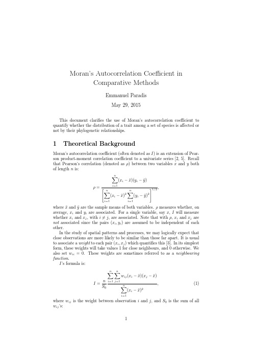
Moran’s Autocorrelation Coefficient inComparative MethodsEmmanuel ParadisMay29,2015This document clarifies the use of Moran’s autocorrelation coefficient to quantify whether the distribution of a trait among a set of species is affected or not by their phylogenetic relationships.1Theoretical BackgroundMoran’s autocorrelation coefficient(often denoted as I)is an extension of Pear-son product-moment correlation coefficient to a univariate series[2,5].Recall that Pearson’s correlation(denoted asρ)between two variables x and y both of length n is:ρ=ni=1(x i−¯x)(y i−¯y)ni=1(x i−¯x)2ni=1(y i−¯y)21/2,where¯x and¯y are the sample means of both variables.ρmeasures whether,on average,x i and y i are associated.For a single variable,say x,I will measure whether x i and x j,with i=j,are associated.Note that withρ,x i and x j are not associated since the pairs(x i,y i)are assumed to be independent of each other.In the study of spatial patterns and processes,we may logically expect that close observations are more likely to be similar than those far apart.It is usual to associate a weight to each pair(x i,x j)which quantifies this[3].In its simplest form,these weights will take values1for close neighbours,and0otherwise.We also set w ii=0.These weights are sometimes referred to as a neighbouring function.I’s formula is:I=nS0ni=1nj=1w ij(x i−¯x)(x j−¯x)ni=1(x i−¯x)2,(1)where w ij is the weight between observation i and j,and S0is the sum of all w ij’s:1S0=ni=1nj=1w ij.Quite not so intuitively,the expected value of I under the null hypothesisof no autocorrelation is not equal to zero but given by I0=−1/(n−1).Theexpected variance of I0is also known,and so we can make a test of the nullhypothesis.If the observed value of I(denotedˆI)is significantly greater thanI0,then values of x are positively autocorrelated,whereas ifˆI<I0,this willindicate negative autocorrelation.This allows us to design one-or two-tailedtests in the standard way.Gittleman&Kot[4]proposed to use Moran’s I to test for“phylogeneticeffects”.They considered two ways to calculate the weights w:With phylogenetic distances among species,e.g.,w ij=1/d ij,where d ijare distances measured on a tree.With taxonomic levels where w ij=1if species i and j belong to the samegroup,0otherwise.Note that in thefirst situation,there are quite a lot of possibilities to setthe weights.For instance,Gittleman&Kot also proposed:w ij=1/dαij if d ij≤cw ij=0if d ij>c,where c is a cut-offphylogenetic distance above which the species are consideredto have evolved completely independently,andαis a coefficient(see[4]fordetails).By analogy to the use of a spatial correlogram where coefficients arecalculated assuming different sizes of the“neighbourhood”and then plotted tovisualize the spatial extent of autocorrelation,they proposed to calculate I atdifferent taxonomic levels.2Implementation in apeFrom version1.2-6,ape has functions Moran.I and correlogram.formula im-plementing the approach developed by Gittleman&Kot.There was an errorin the help pages of?Moran.I(corrected in ver.2.1)where the weights werereferred to as“distance weights”.This has been wrongly interpreted in my book[6,pp.139–142].The analyses below aim to correct this.2.1Phylogenetic DistancesThe data,taken from[1],are the log-transformed body mass and longevity offive species of primates:>body<-c(4.09434,3.61092,2.37024,2.02815,-1.46968)>longevity<-c(4.74493,3.3322,3.3673,2.89037,2.30259)>names(body)<-names(longevity)<-c("Homo","Pongo","Macaca","Ateles","Galago")2The tree has branch lengths scaled so that the root age is one.We read thetree with ape,and plot it:>library(ape)>trnwk<-"((((Homo:0.21,Pongo:0.21):0.28,Macaca:0.49):0.13,Ateles:0.62)" >trnwk[2]<-":0.38,Galago:1.00);">tr<-read.tree(text=trnwk)>plot(tr)>axisPhylo()GalagoAtelesMacacaPongoHomo10.80.60.40.20We choose the weights as w ij=1/d ij,where the d’s is the distances measuredon the tree:>w<-1/cophenetic(tr)>wHomo Pongo Macaca Ateles GalagoHomo Inf2.38095241.02040820.80645160.5Pongo 2.3809524Inf1.02040820.80645160.5Macaca1.02040821.0204082Inf0.80645160.5Ateles0.80645160.80645160.8064516Inf0.5Galago0.50000000.50000000.50000000.5000000InfOf course,we must set the diagonal to zero:>diag(w)<-0We can now perform the analysis with Moran’s I:3>Moran.I(body,w)$observed[1]-0.07312179$expected[1]-0.25$sd[1]0.08910814$p.value[1]0.04714628Not surprisingly,the results are opposite to those in[6]since,there,the distances(given by cophenetic(tr))were used as weights.(Note that the argument dist has been since renamed weight.1)We can now conclude for a slighly significant positive phylogenetic correlation among body mass values for thesefive species.The new version of Moran.I gains the option alternative which specifies the alternative hypothesis("two-sided"by default,i.e.,H1:I=I0).As expected from the above result,we divide the P-value be two if we define H1as I>I0:>Moran.I(body,w,alt="greater")$observed[1]-0.07312179$expected[1]-0.25$sd[1]0.08910814$p.value[1]0.02357314The same analysis with longevity gives:>Moran.I(longevity,w)$observed[1]-0.1837739$expected[1]-0.251The older code was actually correct;nevertheless,it has been rewritten,and is now much faster.The documentation has been clarified.The function correlogram.phylo,which computed Moran’s I for a tree given as argument using the distances among taxa,has been removed.4$sd[1]0.09114549$p.value[1]0.4674727As for body,the results are nearly mirrored compared to[6]where a non-significant negative phylogenetic correlation was found:it is now positive but still largely not significant.2.2Taxonomic LevelsThe function correlogram.formula provides an interface to calculate Moran’s I for one or several variables giving a series of taxonomic levels.An example of its use was provided in[6,pp.141–142].The code of this function has been simplified,and the graphical presentation of the results have been improved.correlogram.formula’s main argument is a formula which is“sliced”,and Moran.I is called for each of these elements.Two things have been changed for the end-user at this level:1.In the old version,the rhs of the formula was given in the order of thetaxonomic hierarchy: e.g.,Order/SuperFamily/Family/Genus.Not re-specting this order resulted in an error.In the new version,any order is accepted,but the order given it is then respected when plotted the correlogram.2.Variable transformations(e.g.,log)were allowed on the lhs of the formula.Because of the simplification of the code,this is no more possible.So it is the responsibility of the user to apply any tranformation before the analysis.Following Gittleman&Kot[4],the autocorrelation at a higher level(e.g., family)is calculated among species belonging to the same category and to dif-ferent categories at the level below(genus).To formalize this,let us write the different levels as X1/X2/X3/.../X n with X n being the lowest one(Genus in the above formula):w ij=1if X k i=X k j and X k+1i =X k+1jw ij=0otherwisek<nw ij=1if X k i=X k j w ij=0otherwisek=nThis is thus different from the idea of a“neighbourhood”of different sizes,but rather similar to the idea of partial correlation where the influence of the lowest level is removed when considering the highest ones[4].To repeat the analyses on the carnivora data set,wefirst log10-transform the variables mean body mass(SW)and the mean female body mass(FW):>data(carnivora)>carnivora$log10SW<-log10(carnivora$SW)>carnivora$log10FW<-log10(carnivora$FW)5We first consider a single variable analysis (as in [6]):>fm1.carn <-log10SW ~Order/SuperFamily/Family/Genus>co1<-correlogram.formula(fm1.carn,data =carnivora)>plot(co1)q q qq−0.20.00.20.40.6M o r a n 's IGenus Family SuperFamily Orderq q P >= 0.05P < 0.05A legend now appears by default,but can be removed with legend =FALSE .Most of the appearance of the graph can be customized via the option of the plot method (see ?plot.correlogram for details).This is the same analysis than the one displayed on Fig.6.3of [6].When a single variable is given in the lhs in correlogram.formula ,an object of class "correlogram"is returned as above.If several variables are analysed simultaneously,the object returned is of class "correlogramList",and the correlograms can be plotted together with the appropriate plot method:>fm2.carn <-log10SW +log10FW ~Order/SuperFamily/Family/Genus >co2<-correlogram.formula(fm2.carn,data =carnivora)>print(plot(co2))6M o r a n 's I −0.20.00.20.40.6Genus FamilySuperFamilyOrderBy default,lattice is used to plot the correlograms on separate panels;using lattice =FALSE (actually the second argument,see ?plot.correlogramList )makes a standard graph superimposing the different correlograms:>plot(co2,FALSE)7−0.20.00.20.40.6M o r a n 's I q q q qqqGenus Family SuperFamily Orderlog10SW log10FWq q P >= 0.05P < 0.05The options are roughly the same than above,but do not have always the same effect since lattice and base graphics do not have the same graphical pa-rameters.For instance,legend =FALSE has no effect if lattice =TRUE .3Implementation in ade4The analysis done with ade4in [6]suffers from the same error than the one done with Moran.I since it was also done with a distance matrix.So I correct this below:>library(ade4)>gearymoran(w,data.frame(body,longevity))class:krandtestMonte-Carlo testsCall:as.krandtest(sim =matrix(res$result,ncol =nvar,byr =TRUE),obs =res$obs,alter =alter,names =s)Test number:2Permutation number:999Alternative hypothesis:greaterTest Obs Std.Obs Pvalue1body -0.062567892.15233420.0012longevity -0.229904370.34614140.414other elements:NULL8The results are wholly consistent with those from ape,but the estimated coefficients are substantially different.This is because the computational meth-ods are not the same in both packages.In ade4,the weight matrix isfirst transformed as a relative frequency matrix with˜w ij=w ij/S0.The weights are further transformed with:p ij=˜w ij−ni=1˜w ijnj=1˜w ij,with p ij being the elements of the matrix denoted as P.Moran’s I isfinally computed with x T P x.In ape,the weights arefirst row-normalized:w ijni=1w ij,then eq.1is applied.Another difference between both packages,though less important,is that in ade4the weight matrix is forced to be symmetric with(W+W T)/2.In ape, this matrix is assumed to be symmetric,which is likely to be the case like in the examples above.4Other ImplementationsPackage sp has several functions,including moran.test,that are more specifi-cally targeted to the analysis of spatial data.Package spatial has the function correlogram that computes and plots spatial correlograms.AcknowledgementsI am thankful to Thibaut Jombart for clarifications on Moran’s I.References[1]J.M.Cheverud,M.M.Dow,and W.Leutenegger.The quantitative as-sessment of phylogenetic constraints in comparative analyses:sexual dimor-phism in body weight among primates.Evolution,39:1335–1351,1985.[2]A.D.Cliffand J.K.Ord.Spatial Autocorrelation.Pion,London,1973.[3]A.D.Cliffand J.K.Ord.Spatial and temporal analysis:autocorrelationin space and time.In E.N.Wrigley and R.J.Bennett,editors,Quantita-tive Geography:A British View,pages104–110.Routledge&Kegan Paul, London,1981.[4]J.L.Gittleman and M.Kot.Adaptation:statistics and a null model forestimating phylogenetic effects.Systematic Zoology,39:227–241,1990. [5]P.A.P.Moran.Notes on continuous stochastic phenomena.Biometrika,37:17–23,1950.[6]E.Paradis.Analysis of Phylogenetics and Evolution with R.Springer,NewYork,2006.9。

moran’s i 指数
Moran'sI指数是一种用于空间数据分析的统计指标，用于衡量
空间相关性的强度和方向。

该指数通常用于地理信息系统和地理统计学中，帮助研究人员了解特定地理区域内不同地点之间的相似性和差异性。

Moran's I指数的值介于-1和1之间，其中负值表示负相关性，正值表示正相关性。

值越接近-1或1表示相关性越强，而值越接近0则表示没有空间相关性。

该指数的计算基于空间自相关性，即某个地点与其周围地点的相似程度。

它涉及到地理空间的权重矩阵，该矩阵定义了每个地点与其周围地点之间的距离和权重关系。

然后使用Moran's I公式计算出指数的值。

Moran's I指数在许多领域都可以应用，包括城市规划，环境研究和社会科学。

它可以帮助研究人员确定特定地理区域内不同地点之间的相似性和差异性，以及空间相关性如何影响各种社会和环境问题。

- 1 -。

空间转录组moransi方法
空间转录组（spatial transcriptomics）是一种用于研究组织中基因表达的技术，它可以提供对细胞类型和基因表达模式的空间分布的信息。

而Moran's I方法是一种用于空间数据的统计分析方法，可用于检测空间相关性。

在空间转录组研究中，Moran's I方法可以用来分析基因表达的空间相关性，以揭示基因在组织中的空间分布模式。

Moran's I方法基于Moran's I统计量，该统计量可以衡量空间数据的空间自相关性。

在空间转录组研究中，可以利用Moran's I方法来分析组织中基因表达的空间分布是否存在聚集现象，从而揭示基因表达的空间相关性。

这有助于我们理解基因在组织中的空间定位和相互作用模式。

Moran's I方法的应用通常涉及到构建空间权重矩阵，该矩阵用于描述不同位置之间的空间关联程度。

然后，通过计算Moran's I统计量来评估基因表达的空间相关性。

这种方法可以帮助研究人员识别在组织中具有显著空间聚集模式的基因，从而深入了解基因在组织结构中的功能和相互关系。

总的来说，空间转录组Moran's I方法提供了一种强大的工具，可以帮助研究人员深入了解基因在组织中的空间分布模式和相互作用，为我们理解生物体内基因表达调控的空间特征提供了重要的信息。

通过Moran's I方法的应用，研究人员可以更全面地认识基因
在组织结构中的功能和调控机制，为生命科学研究提供了新的视角
和方法。