Review Article of Landscape Metrics Based on Remote Sensing Data

格式：pdf
大小：936.68 KB
文档页数：19

下载文档原格式

Fragstats软件中各生态景观指数详述知识讲解

1、指数的选择 :Fragstats/select patch(clas、s land)metrics 指数一共有三个级别， path、class、landscape 三个级别。

不同级别对应不同的指数，对应着不同的生态学意义。

所以选择指数的时候，一定要清楚所选择的指数对应的级别。

2、整理的 Fragstats中可以计算的景观指数注：每个景观指数包含的信息依次为英文缩写——英文全称——指标名称——应用尺度——单位一、面积指标1.A rea/Perimeter①AREA(AREA-CSD 、AREA-CPS、AREA-LS 、AREA-LPS) —Patch Area——斑块面积(类型水平方差、百分比 /景观水平方差、百分比)——斑块—— ha(ha、%) ≥0；2.Isolation/Proximity①LSIM —Landscape Similarity Index—斑块相似系数—斑块—%；3.A rea/Density/Edge①CA —— Total Class Area——斑块类型面积——类型—— ha>0；②PLAND(%LAND) —— Percentage of Landscape——斑块所占景观面积比例——类型——% [0，100]；③T A—— Total Landscape Area——景观面积——景观—ha> 0；④LPI —— Largest Patch Index—最大斑块指数—类型/景观—%；二、密度大小及差异1.A rea/Density/Edge①NP—— Number of Patches——斑块数量——类型 /景观——n ≥1；②PD—— Patch Density——斑块密度——类型/景观——n/100ha；③AREA（AREA-MN 、 AREA-AM 、 AREA-MD 、 AREA-RA 、 AREA-SD 、AREA-CV）（MPS 、PSSD、PSCV）—— Patch Area（Patch Area Mean / Mean Patch Size、Patch Area Standard Deviation / Patch Size Standard Deviation、 Patch Area Coefficient of Variation / Patch Size Coefficient of Variation）——斑块面积（平均斑块面积、面积加权平均斑块面积、斑块面积中值、斑块面积范围、斑块面积标准差、斑块面积变异系数）（平均斑块面积、斑块面积标准差、斑块面积变异系数）——类型 /景观—— ha （ha，%，%）；④GYRA（同上）—Radius of Gyration—回旋半径—类型/景观—m；三、边缘指标 1.Area/Perimeter①PERIM（CSD 、 CPS/LSD、 LPS）—— Patch Perimeter——斑块周长（类型水平方差、百分比 /景观水平方差、百分比）—斑块—m ≥0；②GYRA（同上）——Radius of Gyration——回旋半径—斑块—m；2.C ontrast①EDCON（同上）—— Edge Contrast Index—边缘对比度—斑块—%；3.A rea/Density/Edge①TE—— Total Edge——总边界长度——类型/景观——m；②ED—— Edge Density——边缘密度——类型/景观——m/ha；4.C ontrast①CWED —— Contrast-Weighted Edge Density——对比度加权边缘密度——类型/景观—— m/ha；②TECI —Total Edge Contrast Index—总边缘对比度—类型 /景观—%；③ECI（MN 、AM 、MD 、RA、SD、CV）（MECI 、AWMECI）—— Edge Contrast Index（Mean Edge Contrast Index、Area-Weighted Mean Contrast Index）——边缘对比度（平均、面积加权平均、中值、变化范围、方差、变异系数）（平均边缘对比度、面积加权平均边缘对比度）——类型/景观—— %（ %，%）；四、形状指标1.Shape①PARA（CSD、CPS/LSD、LPS）—— Perimeter Area Ratio——周长面积比（类型水平方差、百分比 /景观水平方差、百分比）—斑块—无；②SHAPE（同上）——Shape Index——形状指标——斑块——无；③FRACT（同上）—— Fractal Dimension Index —分维数—斑块—无；④CRICLE（同上）—— Related Circumscribing Circle—近圆形形状指数——斑块——无；⑤CONTIG（同上）—— Contiguity Index——邻近指数——斑块——无；2.A rea/Density/Edge①LSI — Landscape Shape Inde—x 景观形状指数—类型/景观—无；②NLSI —— Normalize LSI——归一化景观形状指数—类型—无； 3.Shape①PAFRAC—— Perimeter Area Fractal Dimension——周长面积分维——类型/景观——无；②PARA（MN 、AM 、MD 、RA 、SD、CV）——Perimeter Area Ratio——周长面积比（平均、面积加权平均、中值、变化范围、方差、变异系数）——类型/景观——无；③SHAPE（同上）（MSI 、 AWMSI）—— Shape Index （Mean Shape Index、Area-Weighted Mean Shape Index—）—形状指数（平均形状、面积加权的平均形状指标）——类型/景观——无；④FRAC（同上）（MPFD、AWMPFD）—Fractal Dimension Index（Mean Patch Fractal Dimension、Area-Weighted Patch Fractal Dimension—）分维数（平均斑块分维数、面积加权的平均斑块分维数）—类型 / 景观—无；⑤CRICLE（同上））—— Related Circumscribing Circle ——近圆形状指数——类型/景观——无；⑥DLFD —— Double Log Fractal Dimension——双对数分维数——类型/景观——无；五、核心面积指标1.CoreArea①Core（CSD、CPS/LSD、LPS）—— Core Area——核心斑块面积（类型水平方差、百分比 /景观水平方差、百分比）——斑块——ha；②NCORE（同上）—Number of Core Area—核心斑块数量—斑块— n ≥；1③CAI（同上）—Core Area Index—核心斑块面积比指标—斑块—%；2.Core Area①TCA —— Total Core Area——核心斑块总面积—类型/景观—ha；②CPLAND（C%LAND）—Core Area Percentage of Landscape—核心斑块占景观面积比——类型—— % ；③NDCA —— Number of Disjunct Core Area——独立核心斑块数量——类型/景观——n；④DCAD —— Disjunct Core Area Density——独立核心斑块密度——类型/景观——n/100ha；⑤CORE（MN 、AM 、MD 、RA 、SD、CV）（MCA1 、CASD1、CACV1）—Core Area（Mean Core Area、 Core Area Standard Deviation、 Core Area Coefficient of Variation）—核心斑块面积（平均、面积加权平均、中值、变化范围、方差、变异系数）（平均核心斑块面积、核心斑块面积方差、核心斑块面积变异系数）——类型 /景观—— ha（ha,ha,%）；⑥DCA（同上）（MCA2 、CASD2、CACV2）—Disjunct Core Area——独立核心斑块面积（平均独立核心斑块面积、独立核心斑块面积方差、独立核心面积变异系数）——类型/景观——ha（ha,ha,%）；⑦CAI（同上）（MCAI）—— Core Area Index（Mean Core Area Index）—核心斑块面积比指标（平均核心斑块指标）——类型/景观—%；六、邻近度指标1.Isolation/Proximity①PROXIM（CSD 、 CPS/LSD、 LPS）—— Proximity Index—邻近指数（类型水平方差、百分比/景观水平方差、百分比）—斑块—无；②SIMI（同上）—— Similarity Index ——相似度——斑块——无；③ENN（同上）——Euclidean Nearest Neighbor Index——欧氏邻近距离——斑块—— m；2.Isolation/Proximity①PROXIM（MN 、AM 、MD、RA、SD、CV）（MPI）——Proximity Index（Mean Proximity Index）——邻近指数（平均、面积加权平均、中值、变化范围、方差、变异系数）（平均邻近指数）——类型 / 景观——%（%）≥0；②SIMI（同上）—— Similarity Index ——相似度——类型/景观—无；③ENN（同上）（MNN 、 NNSD 、 NNCV）—— Euclidean Nearest Neighbor Index（Mean Euclidean Nearest-Neighbor Index、 Euclidean Nearest-Neighbor Index Standard Deviation 、 Euclidean Nearest-Neighbor Index Coefficient of V ariation）——欧氏邻近距离（平均欧氏邻近距离、欧氏邻近距离方差、欧氏邻近距离变异系数）——类型/景观—— m（m,m,%） >0；七、多样性1.Diversity①PR—— Patch Richness——斑块多度（丰富度）——景观—— n ≥1；②PRD—— Patch Richness Densit——斑块丰富度—景观—n/100ha；③RPR—— Relative Patch Richness——相对丰富度——景观—%；④SHDI—Shannon's Diversity Index—香农多样性指数—景观—无；⑤SIDI —— Simpson's Diversity Index—— Simpson多样性指数——景观——无；⑥MSHDI —— Modified Simpson's Diversity Index—修正Simpson 多样性指数——景观——无；⑦SHEI —— Shannon's Evenness Index——香农均匀度指数—景观—无 [0,1] ；⑧SIEI —— Simpson's Evenness Inde—x — Simpson均匀度指数——景观——无；⑨MSIEI —— Modified Simpson's Evenness Index——修正Simpson 均匀度指数——景观——无；八、聚散性1.Contagion/Interspersion①CLUMPY —— Clumpiness——丛生度——类型—— %；②PLADJ——Proportion of LikeAdjacency ——相似邻近比例——类型/景观——% ( 0,100］；③AI —— Aggregation Index——聚合度—类型/景观— % (0,100］；④IJI—— Interspersion JuxtapositionIndex——散布与并列指数——类型 /景观—— % (0,100］；⑤DIVISIO N —— Landscape DivisionIndex——景观分裂指数——类型/景观——% ( 0,100］；⑥SPLIT —— Splitting Index ——分离度—类型/景观— % (0,100］；⑦MESH—— Effective Mesh Size——有效粒度面积——景观—— % (0,100］；2.Connectivity①COHESION —— Patch Cohesion Index——整体性(斑块凝聚度) ——类型 /景观—— % (0,100］；②CONNECT —Connectance Index——连接度——类型 / 景观—— % (0,100］；3.C ontagion/Interspersion①CONTAG—— Contagion Index—蔓延度——景观—— % (0,100］；。

fragstats please review log message -回复

fragstats please review log message -回复[fragstats please review log message]Introduction:In the world of landscape ecology, the analysis of landscape pattern plays a crucial role in understanding the dynamics and processes of ecological systems. One of the most widely used and powerful tools for landscape pattern analysis is Fragstats. In this article, we will discuss the concept of landscape metrics, explore the functionalities of Fragstats, and provide a step-by-step guide on how to review a log message in Fragstats.1. Understanding Landscape Metrics:Landscape metrics are quantitative measures used to describe the spatial arrangement and composition of landscape elements. These metrics provide valuable information about the structure and function of an ecosystem, aiding in the assessment of landscape health and ecosystem services. Some commonly used landscape metrics include patch density, total edge length, and landscape contagion index.2. Introduction to Fragstats:Fragstats is a software package developed by a team of researchers from the University of Massachusetts. It is designed to analyze landscape patterns and calculate a wide range of landscape metrics. Fragstats can be used for both raster and vector data, making it a versatile tool for various types of landscape studies.3. Step-by-Step Guide on Reviewing Log Messages in Fragstats:Step 1: Launching Fragstats:Start by opening Fragstats on your computer. Once the software is launched, you will be prompted to load your data. Fragstats supports various file formats, including raster images (such as TIFF or IMG) and vector files (such as shapefiles).Step 2: Loading Data:In the Fragstats interface, navigate to the "File" menu and select "Load Data." Browse for the location of your data file and select it. Depending on the size of your dataset, it may take a few moments to load the file into Fragstats.Step 3: Analyzing Landscape Metrics:After the data is loaded, you can proceed to the "Analysis" menu and select the desired landscape metrics from the provided list. Fragstats offers a wide range of metrics, including those related to patch size, shape, and connectivity. Once selected, choose the appropriate options and parameters for the analysis.Step 4: Running the Analysis:Once all the necessary metrics and options are set, click on the "Run" button to initiate the analysis. The software will start processing the dataset and calculating the selected landscape metrics. The progress of the analysis will be displayed in the log message window.Step 5: Reviewing the Log Message:After the analysis is complete, Fragstats generates a log message summarizing the results. To review the log message, go to the "View" menu and select "Log Message." A new window will open where you can read and assess the information provided by Fragstats. The log message contains details about the executed analysis, including the metrics calculated and any warnings or errors encountered.Step 6: Interpreting the Results:Carefully read through the log message to gain insights into the calculated landscape metrics. Focus on the metrics of interest, such as patch size or landscape contagion, and analyze their values within the context of your research objectives. The log message may also provide warnings or errors that could help identify potential issues in the data or analysis process.Conclusion:Fragstats is an invaluable tool for landscape pattern analysis, providing a comprehensive set of metrics to quantify and understand ecological landscapes. By following the step-by-step guide, researchers can effectively review log messages generated by Fragstats to gain insights into the calculated landscape metrics. As landscape ecology continues to evolve, Fragstats remains an essential resource for studying the complex dynamics of ecosystems.。

安徽农业大学景观生态学第一部分2015

景观生态学Landscape Ecology●课程安排第一部分景观生态学的相关概念及发展第二部分景观生态学的理论框架第三部分景观格局第四部分景观生态过程及动态变化第五部分景观生态评价第六部分景观生态学应用第一部分景观生态学的相关概念及发展一.景观生态学相关概念辨析1、第一组概念景观: 景观是土地的具体一部分，代表一种更精细的尺度的含义；更强调供人类观赏的美学价值和作为复杂生命组织整体的生态价值及给人类带来的长期效益。

景观是构成环境的实体部分，既不是环境中所有要素的全部，也不是它们简单相加而成的整体，而是综合的产物。

风景:景观在美学意义上的概念。

包括自然风光、地表形态、风景画面等。

没有明确的空间界限，主要突出一种综合直观的视觉感受。

土地:土地概念侧重于社会经济属性，主要关注的是土地的生产力、土地的产权关系、土地的经济价值等。

环境:环绕于人类周围的客观事物的整体，包括自然因素和社会因素，它们既可以实体形式存在，也可以非实体形式存在。

●景观生态学中的景观✓地理空间概念（19世纪）：A. von Humboldt自然地域综合体：景观是由各种具有空间位置的地理要素组成的地理复杂体（或称地理系统）。

✓生态过程思想（20世纪30年代以来）：Call Troll（1）Naveh (1987): “landscape deal with in their totality as physical, ecological and geographical entities, integrating all natural and human patterns and processes…”.（2）Forman and Godron (1986): landscape as a heterogeneous land area composed of a cluster of interacting ecosystems that is repeated in similar form throughout.”（3）Leser (1997): regards the landscape ecosystem as a spatial pattern of abotic, biotic and anthropogenic components which form a functional entity and serve as human’s environment. （4）肖笃宁（1997）：景观是一个由不同土地单元镶嵌组成，具有明显视觉特征的地理实体；它处于生态系统之上，大地理区域之下的中间尺度；兼具景观、生态和文化的多重价值。

Cultural landscape Landscape metrics Fragmentation Gradient Renaturalization

Landscape and Urban Planning 93 (2009) 250–261Contents lists available at ScienceDirectLandscape and UrbanPlanningj o u r n a l h o m e p a g e :w w w.e l s e v i e r.c o m /l o c a t e /l a n d u r b p l anSpatial context of urbanization:Landscape pattern and changes between 1950and 1990in the Warsaw metropolitan area,PolandJerzy Solon ∗Institute of Geography and Spatial Organization of the Polish Academy of Sciences,00-818Warsaw,Twarda 51/55,Polanda r t i c l e i n f o Article history:Received 25February 2008Received in revised form 3July 2009Accepted 27July 2009Available online 22 August 2009Keywords:Cultural landscape Landscape metrics Fragmentation GradientRe-naturalizationa b s t r a c tThis paper reports on the changes in the spatial structure of landscape in the years 1950–1990within the Warsaw metropolitan area.The analysis was aimed at identiﬁcation of (a)the inﬂuence of the distance from the center of the city and from the transport routes on the values of landscape metrics,(b)changes in time of the landscape metrics of forests and built-up areas,(c)the inﬂuence of habitats,transporta-tion network and the distance from the center on the directions and intensity of urban growth.Several landscape metrics were chosen to describe the landscape pattern (spatial share,mean patch size,patch size coefﬁcient of variance,mean shape index,mean nearest neighbor distance,mean proximity index,and interspersion and juxtaposition index).The majority of changes in land cover took place in the years 1950–1970,but relations between landscape metrics and the distance from the center of Warsaw as well as from the transport routes,had a persistent character over the entire period studied.The inﬂuence of the habitat differentiation (expressed in categories of potential natural vegetation)in land cover is relatively unimportant in the vicinity of the city center and in the direct neighborhood of roads,while it would become the dominating factor in the periphery.The landscape metrics enable the description of the spatial regularities and trends,and constitute useful indirect indicators of the impact of urbanization on cultural (rural)landscape and of the general ecosystem disturbance.© 2009 Elsevier B.V. All rights reserved.1.IntroductionThe rapid and often uncontrolled growth of the urbanized areas brings about numerous changes in the structure and functioning of landscape.These changes concern usually also the areas indi-rectly associated with the expanding agglomerations (the so-called outer suburban zone—Solon,1990),and their spatial extent may be very broad.They are the expression of the general and irreversible process of synanthropization of landscape (understood as struc-tural and functional changes in ecosystems and landscape mosaics,induced directly or indirectly,by various forms of activity of human society—Falinski,1998).Although the process of synanthropization concerns all the components of the environment and all spatial ele-ments of landscape,it is most vividly apparent in the vegetation cover and in land cover.It is held that the most important effects of the process of synan-thropization are fragmentation of habitats and ampliﬁcation of the mosaic character of landscape,simpliﬁcation of composition of the spatial landscape complexes,disappearance of the rare species and ecosystems,decrease of the degree of naturalness of landscape∗Tel.:+48226978930;fax:+48226978903.E-mail address:j.solon@twarda.pan.pl .(Solon,1990).The above statements,although generally true,are in fact a far-reaching generalization.In reality,the processes of landscape transformation under the direct and indirect inﬂuence of urbanization are multi-directional and differentiated in time and space.Li et al.(2003)pointed out that the dynamic process of urban expansion depends very much on topography,transportation net-work in the area,land use,social structure and economic type of the inﬂuenced area,as well as on demography and economy in a city.Ecological consequences of urbanization can be studied directly or indirectly.Direct studies focus on spatial distribution and species composition of different taxa,e.g.,birds (Jokimaki and Kaisanlahti-Jokimaki,2003;Melles et al.,2003),ground arthropods (McIntyre et al.,2001)or vascular ﬂora (Godefroid and Koedam,2003).Indirect studies are mainly aimed at the monitoring of landscape pattern changes and assessment of space suitability for chosen species on the basis of habitat distribution and landscape connectivity (Harms,1999).A more synthetic approach for studying either the process of urbanization or landscape ecological consequences of this process can be designed by quantifying landscape pattern,either based on the analysis of only one index (e.g.,polygon shape index—Comber et al.,2003)or a set of landscape metrics.Different approaches were adopted for this purpose.The most classical of them is urban–rural gradient analysis (Luck and Wu,2002).This method was extended0169-2046/$–see front matter © 2009 Elsevier B.V. All rights reserved.doi:10.1016/ndurbplan.2009.07.012J.Solon/Landscape and Urban Planning93 (2009) 250–261251by incorporation of temporal trends analysis(Weng,2007),and multiplication of transects(Kong and Nakagoshi,2006;Yu and Ng, 2007).The other approach,based on grid analysis for the entire landscape,ﬁlls in the information gaps that arise by only presenting a cross-section of the study area(Hahs and McDonnell,2006).Landscape metrics combined with gradient analysis or with entire landscape analysis,aimed at describing landscape changes under the inﬂuence of urbanization,were applied for several cities or regions,mainly North American(Medley et al.,1995;Jenerette and Wu,2001;Luck and Wu,2002;Herold et al.,2003;Dietzel et al.,2005;Ji et al.,2006;DiBari,2007;Weng,2007),Asiatic(Zhang et al.,2004;Abdullah and Nakagoshi,2006;Kong and Nakagoshi, 2006;Yu and Ng,2007;Huang et al.,2009),and Australian(Hahs and McDonnell,2006).For European cities similar research is not known to the Author,except for the global comparative analysis for 77metropolitan areas(14of them were European)(Huang et al., 2007).The purpose of the study here presented is to show the changes in the spatial structure of landscape in the years1950–1990within the former voivodship(province)of Warsaw.The analysis was aimed to answer the following questions:(a)what is the inﬂuence of the distance from the center of the city and from the transport routes on the values of landscape metrics?(b)how do the land-scape metrics of forests and built-up areas change over time?(c)is it possible to determine the inﬂuence of habitats,the transporta-tion network,and the distance from the center on the directions and intensity of urban growth?At the background of this study lies an assumption that the landscape structure is shaped by different processes,occurring simultaneously at the same area,or separately in different parts of the region.The former studies identiﬁed three main pro-cesses taking place within the study area:(a)urbanization,(b) re-naturalization(restoration)connected with nature protection, and(c)abandonment of rural areas—which was not important before1970(Gutry-Korycka,2005).In this light,the identiﬁca-tion of threshold distance at which urbanization ceases to be the main factor shaping the landscape,is the additional objective of the study.2.Study areaThe analyzed area,forming the core part of Warsaw metropoli-tan area,corresponds to the capital province(voivodship)of Warsaw from the years1975to1998.This area encompasses about 3800km2within the radius of20km(in NE direction)to50km (NW direction)from the center of the city of Warsaw.The popula-tion of the area grew up from1.26million in1950to2.43million in2000.The study area is divided into73administrative units (Fig.1).One of them(Warsaw-Centrum)is the most urbanized,core unit of the agglomeration;the subsequent11units constitute the rest of Warsaw city.Among61units surrounding the proper city there are35administrative units of rural character,and26small towns.The region encompasses the valley of the Vistula river with its ﬂood terrace of the altitude of roughly78m a.s.l.,the over-ﬂood terraces with sandy plains and dunes,as well as the denuded post-glacial upland situated at more than100m a.s.l.In accordance with the geo-botanical regional division of Poland (Matuszkiewicz,1993)the study area belongs to two geo-botanical provinces:the Northern Masovian-Kurpie Province,and the South-ern Masovian-Podlasie Province(divided into several districts). This area isﬂoristically relatively poor,and,in addition,it is located outside of the natural range of beech,spruce,andﬁr.The city of Warsaw is located at the interface of four geo-botanical districts and seven sub-districts,differing as to the surface shares of the particular habitat types.The habitat diversity of the area is high(Solon,1994)and it includes at least17types of habitats,corresponding to the types of the potential natural vegetation(in the sense of Tüxen,1956),featuring different ecological requirements:high moors(Oxycocco-Sphagnetea),boggy and humid pine forests(Vac-cinio uliginosi-Pinetum and Molinio-Pinetum),dry pine forests (Cladonio-Pinetum),typical pine forests(Peucedano-Pinetum and Leucobryo-Pinetum),alder forests(Ribo nigri-Alnetum and Sphagno-Alnetum),willow-and-poplarﬂoodplain forests(Salici-Populetum), ash-and-alderﬂoodplain forests(Fraxino-Alnetum),ash-and-elm ﬂoodplain forests(Ficario-Ulmetum typicum),elmﬂoodplain forests (Ficario-Ulmetum chrysosplenietosum),hornbeam forests(Tilio-Carpinetum),split up into the poor and fertile series,xerothermic oak woods(Potentillo albae-Quercetum),and mixed pine forests (Querco roboris-Pinetum and Serratulo-Pinetum).Theﬁrst four habi-tats occupy very limited areas.In connection with the diversity of habitats and types of land use,the actual vegetation is relatively rich in syntaxo-nomic terms,but highly fragmented in space.Thus,altogether more than100local phytocoenons(types of plant communi-ties)were identiﬁed,most of them at the level of association or lower.They belong to12phytosociological classes:Epilobi-etea,Artemisietea,Phragmitetea,Koelerio-Corynephoretea,Molinio-Arrhenatheretea,Scheuchzerio-Caricetea nigrae,Nardo-Callunetea, Rhamno-Prunetea,Salicetea purpureae,Alnetea glutinosae,Vaccinio-Piceetea and Querco-Fagetea.Many of the plant associations occupy very small surfaces(with separate patches covering only some hundreds of square meters and representing jointly no more than1%of the whole area). This restricted distribution is highly correlated with thefragmen-Fig.1.Location of the study area.252J.Solon/Landscape and Urban Planning93 (2009) 250–261Table1Land cover(in ha)distribution on the study area.Year195019701990Grasslands31,83226,71426,657 Forests51,34191,05692,346 Arable lands24,197518,524817,5159 Orchards2,4344,6635,557 Water10,38111,46811,949 Built-up41,43560,24967,730tation of the terrain,and so they can only be analyzed at very detailed scales.An example can be provided by the commune of Łomianki,where on the area of38km2the presence of81phyto-coenons was observed,of which only around30occupied surfaces exceeding2–5%of the whole area for each vegetation type(Solon, 1994).3.MethodsThe analysis was based upon the digital maps of land cover for the years1950,1970and1990(maps were prepared by vector-izing the1:25,000paper sheets).For each of these time instants numerous information layers were available(forming separateﬁles in the.shp format),of which the following ones were used:built-up areas(polygons),elements of land cover(polygons),surface waters (polygons),railway network(lines),road network(lines).In addi-tion,the map of potential natural vegetation(polygons)was used, which was specially digitized from the1:300,000paper version edited by Matuszkiewicz et al.(1995).Detailed information about source maps,vectorizing procedure,and preparation of the spatial database is available in Gutry-Korycka(2005).The work on these materials proceeded in several stages.The ﬁrst one consisted of the transformation of the source maps and encompassed the following steps:(a)elaboration for each time instant analyzed(1950,1970and1990)of a land cover map as resulting from the superposition of the maps of built-up areas,sur-face waters and land cover elements;(b)elaboration of two polygon maps of equal distance contours with the step of2km,ﬁrst–from the commune of Warsaw-Center,and second–from the selected (main,ﬁrst order)roads and all railway lines.All roads and railroads taken into account were constructed before1950.Thereafter,the three maps of land cover were overlaid succes-sively on and intersected with the three maps showing the surfaces of reference(two maps of equal distance contours and the map of potential vegetation).In this manner,nine derived maps were obtained,and their attribute tables were used for different calcula-tions.The generation of maps of equal distance contours,and their intersection with land cover maps were the main points in the method of the equal-distance area analysis,which was applied in this study.In the second stage of analysis the selected indices(metrics)of landscape composition and conﬁguration(McGarigal and Marks, 1995)were calculated for all the derived maps(accounting for the two generalized categories of land cover:forests and built-up areas).The calculations were carried out with the Patch Analyst extension for ArcView3.3.These were the following metrics:spa-tial share(Share),mean patch size(MPS),patch size coefﬁcient of variance(PSCOV),mean shape index(MSI),mean nearest neighbor distance(MNND),mean proximity index(MPI),and interspersion and juxtaposition index(IJI).For obtaining the spatial representation of areas on which land cover has changed,three maps of land cover(for years1950,1970 and1990)were overlaid and intersected.The output shapeﬁle was inspected,and the histogram of frequencies of polygon area classes was constructed.On this basis the group of the smallest polygons was selected.These polygons were treated as artifacts of slightly different boundaries for each time frame and thus excluded from the further analysis.4.Results4.1.General trends of land cover changesDuring the forty years analyzed important changes took place in the land cover.There has been a very clear upward trend in the shares of forests and built-up areas,whose surfaces increased by,respectively,around80%and63%in comparison with the area occupied in1950.On the other hand,there has been a drop in the area shares of arable land and the permanent grasslands,by, respectively,28%and16%.It should be noted that the most impor-tant changes took place in theﬁrst twenty years,while the period 1970–1990was characterized by a distinct slow down of the rate of changes(Table1).The increase of the forest areas occurred primarily at the cost of theﬁeld areas during the period1950–1970.More than15%of the surface of theﬁelds in1950changed to forest,and then in the period 1970–1990only a bit less than2%of theﬁeld areas in1970changed to forest(Table2).Forestation also took place on almost1700ha of the compact and dispersed village structures.This process tookTable2Land cover transition matrices for years1950–1970and1970–1990.Theﬁgures in the matrix show the area(in ha)of each older(year on the left side)land cover type that had become transformed to newer(year in the upper row)land cover types.Area(in ha)in1970Grasslands Forests Arable lands Orchards Water Built-up Area(in hectares)in1950Grasslands16,7473,8469,1481201,351620Forests30647,7501,6671741541,290Arable lands8,90536,95916,27843,6743,3942,6259Orchards373831,22644416328Water4418322,408446,464192Built-up2781,2868,0152078931,560Area(in ha)in1990Grasslands Forests Arable lands Orchards Water Built-up Area(in hectares)in1970Grasslands24,0105711,646122202163Forests7188,4461,7166675682Arable lands2,5752,94017,11511,4252046,953Orchards005333,9440186Water000011,4680Built-up138********,746J.Solon/Landscape and Urban Planning93 (2009) 250–261253place within the territory of the Kampinos National Park and was associated with the buying out of private land and controlled re-naturalization of the forest and swamp complex(Lenartowicz and Markowski,2004).The increase of the area of built-up surfaces was proceeding in a similar manner.By1970built-up areas covered roughly11%of the area ofﬁelds,existing in1950,while in the period1970–1990 built-up areas transformed close to3%of theﬁeld areas from1970. Of other signiﬁcant changes in land cover one should mention the increase of water surfaces by10%in the years1950–1970,which was due to the construction of the artiﬁcial reservoir(Zegrze Reser-voir)on river Narew(Plit and Solon,1990)(Table2).A more detailed analysis of the transition matrix(Table2)indicates a differentiated persistence of the particular types of land cover.Most variable was the spatial distribution of orchards,of which only18%of the area occupied in1950was still under orchard use in1970(although their total area increased almost twice in the same period).The most per-sistent in theﬁrst twenty years were forests(93%of the forest area of1950has not changed),while in the second twenty years most persistent were forests and built-up areas—respectively,97%and 99%of area has not undergone changes in terms of use.Altogether, in the entire period of1950–1990land cover changed at least once over more than33%of the whole area studied.Most persistent were forests,followed by the built-up areas,waters,arable land,grass-lands and orchards(respectively:92%,76%,70%,65%,50%and14% of the area occupied initially by a given land cover form has not changed during forty years).The biggest changes in land cover took place in the vicinity of Warsaw and in the river valleys,as well as on the relatively unfer-tile sandy habitats(Fig.2).Despite a signiﬁcant decrease of the area,the general landscape role of theﬁeld areas has not under-gone a drastic change.Both in1950and in1990ﬁelds constituted isolated patches(islands)in the vicinity of Warsaw,while in many peripheral areas they had the character of the background(matrix). There has been a distinct change in the role of built-up areas,espe-cially along the transport lines.In1950the built-up areas formed isolated patches,and the entire landscape had a mosaic structure. Since1970the majority of the built-up areas grew and merged, forming vast and continuous structure having the character of the background(matrix),in which smaller patches of other types of land cover are immersed.4.2.Distribution of forests and built-up areas on different habitatsDuring the analyzed period of forty years the forests have been–and are–most tightly associated with two types of habi-tats of potential vegetation:the dry and acid habitats of pine forests(1—Peucedano-Pinetum and Leucobryo-Pinetum)and mixed pine forests(2—Querco-Pinetum)(where their share reaches80% of the habitat area),and the strongly humid or wet alder habi-tats(9—Ribo-Alnetum).The high value for xerophilous oak forest (3—Potentillo-Quercetum)is connected with the only patch of this community.On the medium humid and fertile habitats,most advantageous for agricultural purposes,their share ranged from 1%to20%of the habitat area(Fig.3a).The lowest value of the mean patch size is characteristic for for-est patches existing on habitats most advantageous for agricultural purposes,i.e.oak-hornbeam forest habitat(5—Tilio-Carpinetum fertile form),and elm-and-ashﬂoodplain forest habitat(6—Ficario-Ulmetum typicum)(Fig.3b).It should be emphasized that the process of fragmentation and disappearance of forests took place in the oak-hornbeam forest habitats much earlier than the starting point of our analysis,although in the period1970–1990the average size of patches started to grow again.The built-up areas are associated primarily with fertile habitats (3—Potentillo-Quercetum,4—Tilio-Carpinetum poor form,5—Tilio-Fig.2.General differentiation of potential natural vegetation(upperﬁgure)and areas,over which the type of land cover has not changed in the years1950–1990 (lowerﬁgure).Legend for the upperﬁgure:1—Peucedano-Pinetum and Leucobryo-Pinetum;2—Querco-Pinetum;3—Potentillo-Quercetum;4—Tilio-Carpinetum poor form;5—Tilio-Carpinetum fertile form;6—Ficario-Ulmetum typicum;7—Fraxino-Alnetum;8—Salici-Populetum;9—Ribo-Alnetum.Carpinetum fertile form),where they occupy up to40%of the available habitat area(Fig.3c).The relatively high share of the built-up areas on the pine forest and mixed pine forest habitats(up to 20%of the respective habitat area)is the effect of the existence of old localities which initially had the character of spas and health resorts(like,for instance,in the vicinity of Otwock).The mean patch size of built-up areas was relatively stable over the study period(Fig.3d).The only excep-tions were habitats of xerophilous oak forest(3—Potentillo-Quercetum)and oak-hornbeam forest(5—Tilio-Carpinetum fertile form)on which mean patch size of built-up areas regularly increased.254J.Solon /Landscape and Urban Planning93 (2009) 250–261Fig.3.Occurrence of forests (left column)and built-up areas (right column)on different habitats of potential natural vegetation.Habitats:1—Peucedano -Pinetum and Leucobryo -Pinetum ;2—Querco -Pinetum ;3—Potentillo -Quercetum ;4—Tilio -Carpinetum poor form;5—Tilio -Carpinetum fertile form;6—Ficario -Ulmetum typicum ;7—Fraxino -Alnetum ;8—Salici -Populetum ;9—Ribo -Alnetum .Habitats are ordered from the poorest and the driest (Peucedano -Pinetum )to the wettest and more fertile.4.3.Spatial pattern of forests relative to the distance from the city center and main roads and railroads4.3.1.Spatial pattern of forests relative to the distance from the city centerIrrespective of the relationship between the habitats of poten-tial vegetation and the real forest land cover,the distribution and characteristics of forest patches has been clearly associated with the distance from the center of Warsaw (Fig.4).The percentage of forests systematically increases along with the distance from the city center.Such a pattern of spatial distribution concerns all the years analyzed,with a general increase of forest area hav-ing taken place in the years 1950–1970:by some 5%close to the center and by around 10%within the peripheries (Fig.4a).The rela-tion between the distance considered and the mean size of forest patches has a different nature.The largest forest patches appear at the distance of 4–6km from the center.In this context,a distinct increase of the mean patch area has been observed in the years 1950–1970at smaller distances from the center,with almost no changes within the peripheries (Fig.4b).Variability of patch size has a similar character in all time-periods;it is the lowest close to the center and increases with the distance (with downward ﬂuc-tuation in the 4–6and 10–12km distance),having a weakening increase at the distance of some 18km from the center.It should be emphasized that in the period 1950–1970there has been a strong increase of the differentiation of forest patch sizes in the closest vicinity of the center (at the distance of 0–4km)and a slight decrease at the distance of 4–6km (Fig.4c).Mean shape index of the forests was in all the sub-periods weakly associated with the distance from the center and displayed an oscillatory behav-ior,with the patches having most irregular shapes appearing in 1950in the nearest vicinity of the center,and then,in later years,at the distance of 4–8km from the center (Fig.4d).In 1950the average patch to patch distance showed little variability (only atthe distance 8–16km it ﬂuctuated in the range of 800–1400m),while in the later periods the values of MNND demonstrate that closest to the center of Warsaw (0–8km)the distance between patches distinctly decreased,while in the remaining area it was more variable (Fig.4e).The number and the mean size of patches,as well as the distances between the patches inﬂuence the values of the mean proximity index (MPI),which measures the degree of isolation and fragmentation of the given patch type.In 1950the values of MPI were,in general,very low,and this was irre-spective of the distance from the city center.In the period until 1970there had been a signiﬁcant increase of the value of this index (particularly within the distance of 4km from the center),signifying the drop of the degree of isolation between the forest patches.In the years 1970–1990the spatial structure underwent only a slight modiﬁcation,expressed through a small decrease of the MPI value with respect to the year 1970(Fig.4f).Spatial vari-ability of the IJI index is highly speciﬁc.Low values of this index exist both at the close distances from the center and within the peripheries.On the other hand,at the distance of 4–18km,the index takes higher values,which vary little.An identical spatial pattern is observed for all the periods analyzed,though in 1950the values of the index were generally lower than in the years 1970and 1990(Fig.4g).4.3.2.Spatial pattern of forests relative to the distance from the main roads and railroadsThe percentage of the forests is almost invariable at the distance of up to 8km from the transport routes and increases considerably at bigger distances (Fig.4h).Such a pattern of spatial distribution is observed in all the years analyzed,with the increase of the forest area by roughly 10%in every sector considered,having taken place between the years 1950and 1970.A very similar spatial differen-tiation is shown by mean patch size:limited variability up to the distance of 8km and a strong increase for bigger distances.In addi-J.Solon/Landscape and Urban Planning93 (2009) 250–261255tion,it was observed that in the years1950–1970a small increase of the mean patch size took place close to the roads and a decrease at the distance of10–12km from them(Fig.4i).Variability of patch sizes has a similar character in the years1970and1990:it is the lowest close to the transport routes and increases along with the distance from them,with a slight downward tendency at the dis-tance of more than10km from the roads.This pattern of variability is clearly different from the one observed for the year1950.At that time,variability of the patch sizes was much smaller,with the local maxima at the distance of4–6km from the roads(Fig.4j).The mean shape index of the forest patches was in1950clearly associated with the distance from the transport routes:the regularly shaped patches dominated close to the roads,while patches of a much more fragmented shape were situated at the distances of at least8km.In 1970the value of MSI close to the transport routes increased,while it somewhat decreased at distances of2–10km beforeincreasing Fig.4.Values of selected landscape metrics of forest patches as depending upon the distance from the city center(left column)and the main roads(right column).256J.Solon /Landscape and Urban Planning93 (2009) 250–261Fig.4.(Continued ).slightly.Such a tendency of changes also appeared (although with a lower intensity)in 1990,which caused that at the end of this period the maximum mean value of MSI was observed at the distance of 4–6km (Fig.4k).In 1950the average distance from patch to patch was low with little variability at the distance up to 10km from the roads,while it was almost four times higher 10–12km away.In the later periods the values of MNND in the vicinity of roads have almost not changed,but they have substantially dropped at the dis-tances exceeding 10km (Fig.4l).On the other hand,the degree of isolation and fragmentation of the forest patches (MPI index)devel-oped quite differently in particular periods.In 1950the values of MPI were generally low and very low,irrespective of the distance from the roads.In 1970a signiﬁcant increase of the index value took place,especially pronounced at the distances greater than 8km。

fragstats景观格局指数归纳

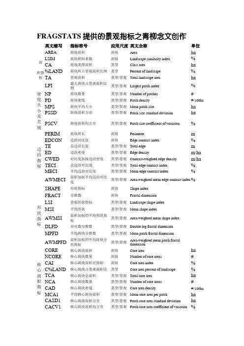
FRAGSTATS提供的景观指标之青柳念文创作英文缩写指标称号应用尺度英文全称单位面积指标AREA斑块面积斑块Area ha LSIM斑块相似系数斑块Landscape similarity index% CA斑块类型面积类型Class area ha %LAND斑块所占景观面积比例类型Percent of landscape% TA景观面积类型/景观Total landscape area ha LPI最大斑块占景观面积比例类型/景观Largest patch index%密度大小及差别NP斑块数量类型/景观Number of patches#PD斑块密度类型/景观Patch density#/100ha MPS斑块平均大小类型/景观Mean patch size ha PSSD斑块面积方差类型/景观Patch size standard deviation ha PSCV斑块面积均方差类型/景观Patch size coefficient of variation%边沿指标PERIM斑块周长斑块Perimeter m EDCON边沿对比度斑块Edge contrast index% TE总边沿长度类型/景观Total edge m ED边沿密度类型/景观Edge density m/ha CWED对比度加权边沿密度类型/景观Contrast-weighted edge density m/ha TECI总边沿对比度类型/景观Total edge contrast index% MECI平均边沿对比度类型/景观Mean edge contrast index% AWMECI面积加权平均边沿对比度类型/景观Area-weighted mean edge contrast index%形状指标SHAPE形状指标斑块Shape indexFRACT分维数斑块Fractal dimensionLSI景观形状指标类型/景观Landscape shape indexMSI平均形状类型/景观Mean shape indexAWMSI面积加权的平均形状指标类型/景观Area-weighted mean shape index DLFD双对数分维数类型/景观Double log fractal dimension MPFD平均斑块分维数类型/景观Mean patch fractal dimensionAWMPFD面积加权的平均斑块分形指标类型/景观Area-weighted mean patch fractaldimension核心面积指标CORE核心斑块面积斑块Core area ha NCORE核心斑块数量斑块Number of core areas# CAI核心斑块面积比指标斑块Core area index% C%LAND核心斑块占景观面积比类型Core area percent of landscape% TCA核心斑块总面积类型/景观Total core area ha NCA核心斑块数量类型/景观Number of core areas# CAD核心斑块密度类型/景观Core area density#/100ha MCA1平均核心斑块面积类型/景观Mean core area per patch ha CASD1核心斑块面积方差类型/景观Patch core area standard deviation ha CACV1核心斑块面积均方差类型/景观Patch core area coefficient of variation%MCA2独立核心斑块平均面积类型/景观Mean area per disjunct core ha CASD2核心斑块面积方差类型/景观Disjunct core area standard deviation ha CACV2核心斑块面积均方差类型/景观Disjunct core area coefficient ofvariation% TCAI总核心斑块指标类型/景观Total core area index% MCAI平均核心斑块指标类型/景观Mean core area index%临近度指标NEAR最临近间隔斑块Nearest-nei**or distance m PROXIM临近指标斑块Proximity indexMNN平均最近间隔类型/景观Mean nearest –nei**or distance m NNSD最临近间隔方差类型/景观Nearest-nei**or standard deviation m NNCV最临近间隔尺度差类型/景观Nearest-nei**or coefficient of variation MPI平均临近度指标类型/景观Mean proximity index%多样性指标SHDI香农多样性指标景观Shannon’s diversity indexSIDI Simpson多样性指标景观Simpson’s diversity indexMSIDI修正Simpson多样性指标景观Modified Simpson’s diversity indexPR斑块多度（景观丰度）景观Patch richness# PRD斑块多度密度景观Patch richness density#/100ha RPR相对斑块多度景观Relative patch richness% SHEI香农平均度指标景观Shannon’s evenness indexSIEI Simpson平均度指标景观Simpson’s evenness indexMSIEI修正Simpson平均度指标景观Modified Simpson’s evenness index离合性IJJ散布与并列指标类型/景观Interspersion and Juxtaposition index% CONTAG舒展度指标景观Contagion index%斑块类型面积（CA），单位：ha，范围：CA>0 （2-1）公式描绘：CA等于某一斑块类型中所有斑块的面积之和（m2），除以10000后转化为公顷（ha）；即某斑块类型的总面积.生态意义：CA度量的是景观的组分，也是计算其它指标的基础.它有很重要的生态意义，其值的大小制约着以此类型斑块作为聚居地（Habitation）的物种的丰度、数量、食物链及其次生种的繁殖等，如许多生物对其聚居地最小面积的需求是其生存的条件之一；分歧类型面积的大小可以反映出其间物种、能量和养分等信息流的差别，一般来讲，一个斑块中能量和矿物养分的总量与其面积成正比；为了懂得和管理景观，我们往往需要懂得斑块的面积大小，如所需要的斑块最小面积和最佳面积是极其重要的两个数据.景观面积（TA），单位：ha，范围：TA>0（2-2）公式描绘：TA等于一个景观的总面积，除以10000后转化为公顷（ha）.生态意义：TA决议了景观的范围以及研究和分析的最大尺度，也是计算其它指标的基础.在自然呵护区设计和景观生态建设中，对于维护高数量的物种，维持稀有种、濒危种以及生态系统的稳定，呵护区或景观的面积是最重要的因素.斑块所占景观面积的比例（%LAND），单位：百分比，范围：0<%LAND<=100（2-3）公式描绘：%LAND等于某一斑块类型的总面积占整个景观面积的百分比.其值趋于0时，说明景观中此斑块类型变得十分稀少；其值等于100时，说明整个景观只由一类斑块组成.生态意义：%LAND度量的是景观的组分，其在斑块级别上与斑块相似度指标（LSIM）的意义相同.由于它计算的是某一斑块类型占整个景观的面积的相对比例，因而是帮忙我们确定景观中模地（Matrix）或优势景观元素的依据之一；也是决议景观中的生物多样性、优势种和数量等生态系统指标的重要因素.斑块个数（NP），单位：无，范围：NP>=1NP = n （2-4）公式描绘：NP在类型级别上等于景观中某一斑块类型的斑块总个数；在景观级别上等于景观中所有的斑块总数.生态意义：NP反映景观的空间格局，常常被用来描绘整个景观的异质性，其值的大小与景观的破碎度也有很好的正相关性，一般规律是NP大，破碎度高；NP 小，破碎度低.NP对许多生态过程都有影响，如可以决议景观中各种物种及其次生种的空间分布特征；改变物种间相互作用和协同共生的稳定性.而且，NP对景观中各种干扰的舒展程度有重要的影响，如某类斑块数目多且比较分散时，则对某些干扰的舒展（虫灾、火灾等）有抑制作用.最大斑块所占景观面积的比例（LPI），单位：百分比，范围：0<LPI<=100（2-5）公式描绘：LPI等于某一斑块类型中的最大斑块占据整个景观面积的比例.生态意义：有助于确定景观的模地或优势类型等.其值的大小决议着景观中的优势种、外部种的丰度等生态特征；其值的变更可以改变干扰的强度和频率，反映人类活动的方向和强弱.斑块平均大小（MPS），单位：ha，范围：MPS>0 （2-6）公式描绘：MPS在斑块级别上等于某一斑块类型的总面积除以该类型的斑块数目；在景观级别上等于景观总面积除以各个类型的斑块总数.生态意义：MPS代表一种平均状况，在景观布局分析中反映两方面的意义：景观中MPS值的分布区间对图像或地图的范围以及对景观中最小斑块粒径的选取有制约作用；另外一方面MPS可以指征景观的破碎程度，如我们认为在景观级别上一个具有较小MPS值的景观比一个具有较大MPS值的景观更破碎，同样在斑块级别上，一个具有较小MPS值的斑块类型比一个具有较大MPS 值的斑块类型更破碎.研究发现MPS值的变更能反馈更丰富的景观生态信息，它是反映景观异质性的关键.面积加权的平均形状因子（AWMSI），单位：无，范围：AWMSI>=1 （2-7）公式描绘：AWMSI在斑块级别上等于某斑块类型中各个斑块的周长与面积比乘以各自的面积权重之后的和；在景观级别上等于各斑块类型的平均形状因子乘以类型斑块面积占景观面积的权重之后的和.其中系数0.25是由栅格的基本形状为正方形的定义确定的.公式标明面积大的斑块比面积小的斑块具有更大的权重.当AWMSI=1时说明所有的斑块形状为最简单的方形（采取矢量版本的公式时为圆形）；当AWMSI值增大时说明斑块形状变得更复杂，更不规则.生态意义：AWMSI是度量景观空间格局复杂性的重要指标之一，并对许多生态过程都有影响.如斑块的形状影响动物的迁移、寻食等活动]，影响植物的种植与生产效率；对于自然斑块或自然景观的形状分析还有另外一个很显著的生态意义，即常说的边沿效应.面积加权的平均斑块分形指数（AWMPFD），单位：无，范围：1<=AWMPFD<=2 （2-8）公式描绘：AWMPFD的公式形式与AWMSI相似，分歧的是其运用了分维实际来丈量斑块和景观的空间形状复杂性.AWMPFD=1代表形状最简单的正方形或圆形，AWMPFD=2代表周长最复杂的斑块类型，通常其值的可以上限为1.5.生态意义：AWMPFD是反映景观格局总体特征的重要指标，它在一定程度上也反映了人类活动对景观格局的影响.一般来讲，受人类活动干扰小的自然景观的分数维值高，而受人类活动影响大的人为景观的分数维值低.应该指出的是，虽然分数维指标被越来越多地运用于景观生态学的研究，但由于该指标的计算成果严重依赖于空间尺度和格网分辨率，因而我们在操纵AWMPFD指标来分析景观布局及其功能时要更为审慎.平均最近间隔（MNN），单位：m，范围：MNN>0 （2-9）公式描绘：MNN在斑块级别上等于从斑块ij到同类型的斑块的最近间隔之和除以具有最近间隔的斑块总数；MNN在景观级别上等于所有类型在斑块级别上的MNN之和除以景观中具有最近间隔的斑块总数.生态意义：MNN度量景观的空间格局.一般来讲MNN值大，反映出同类型斑块间相隔间隔远，分布较团圆；反之，说明同类型斑块间相距近，呈团聚分布.别的，斑块间间隔的远近对干扰很有影响，如间隔近，相互间容易发生干扰；而间隔远，相互干扰就少.但景观级别上的MNN在斑块类型较少时应慎用.平均临近指数（MPI），单位：无，范围：MPI>=0 （2-10）公式描绘：给定搜索半径后，MPI在斑块级别上等于斑块ijs 的面积除以其到同类型斑块的最近间隔的平方之和除以此类型的斑块总数；MPI在景观级别上等于所有斑块的平均临近指数.MPI=0时说明在给定搜索半径内没有相同类型的两个斑块出现.MPI的上限是由搜索半径和斑块间最小间隔决议的.生态意义：MPI可以度量同类型斑块间的邻远程度以及景观的破碎度，如MPI值小，标明同类型斑块间团圆程度高或景观破碎程度高；MPI值大，标明同类型斑块间临近度高，景观毗连性好.研究证明MPI对斑块间生物种迁徙或其它生态过程停顿的顺利程度都有十分重要的影响.景观丰度（PR），单位：无，范围：PR>=1（2-11）公式描绘：PR 等于景观中所有斑块类型的总数.生态意义：PR是反映景观组分以及空间异质性的关键指标之一，并对许多生态过程发生影响.研究发现景观丰度与物种丰度之间存在很好的正相关，特别是对于那些生存需要多种生境条件的生物来讲PR就显得尤其重要.香农多样性指数（SHDI），单位：无，范围：SHDI>=0（2-12）公式描绘：SHDI在景观级别上等于各斑块类型的面积比乘以其值的自然对数之后的和的负值.SHDI=0标明整个景观仅由一个斑块组成；SHDI增大，说明斑块类型增加或各斑块类型在景观中呈平衡化趋势分布.生态意义：SHDI是一种基于信息实际的丈量指数，在生态学中应用很广泛.该指标能反映景观异质性，特别对景观中各斑块类型非平衡分布状况较为敏感，即强调稀有斑块类型对信息的贡献，这也是与其它多样性指数分歧之处.在比较和分析分歧景观或同一景观分歧时期的多样性与异质性变更时，SHDI也是一个敏感指标.如在一个景观系统中，土地操纵越丰富，破碎化程度越高，其不定性的信息含量也越大，计算出的SHDI值也就越高.景观生态学中的多样性与生态学中的物种多样性有慎密的接洽，但其实不是简单的正比关系，研究发现在一景观中二者的关系一般呈正态分布.香农均度指数（SHEI），单位：无，范围：0<=SHEI<=1（2-13）公式描绘：SHEI等于香农多样性指数除以给定景观丰度下的最大可以多样性（各斑块类型均等分布）.SHEI=0标明景观仅由一种斑块组成，无多样性；SHEI=1标明各斑块类型平均分布，有最大多样性.生态意义：SHEI与SHDI指数一样也是我们比较分歧景观或同一景观分歧时期多样性变更的一个有力手段.而且，SHEI与优势度指标（Dominance）之间可以相互转换（即evenness=1-dominance）,即SHEI值较小时优势度一般较高，可以反映出景观受到一种或少数几种优势斑块类型所支配；SHEI趋近1时优势度低，说明景观中没有分明的优势类型且各斑块类型在景观中平均分布.散布与并列指数（IJI），单位：百分比，范围：0<IJI<=100 （2-14）公式描绘：IJI在斑块类型级别上等于与某斑块类型i相邻的各斑块类型的邻接边长除以斑块i的总边长再乘以该值的自然对数之后的和的负值，除以斑块类型数减1的自然对数，最后乘以100是为了转化为百分比的形式；IJI在景观级别上计算各个斑块类型间的总体散布与并列状况.IJI取值小时标明斑块类型i仅与少数几种其它类型相邻接；IJI=100标明各斑块间比邻的边长是均等的，即各斑块间的比邻概率是均等的.生态意义：IJI是描绘景观空间格局最重要的指标之一.IJI对那些受到某种自然条件严重制约的生态系统的分布特征反映显著，如山区的各种生态系统严重受到垂直地带性的作用，其分布多呈环状，IJI值一般较低；而干旱区中的许多过渡植被类型受制于水的分布与多寡，彼此临近，IJI值一般较高.舒展度指数（CONTAG），单位：百分比，范围：0<CONTAG<=100（2-15）公式描绘：CONTAG 等于景观中各斑块类型所占景观面积乘以各斑块类型之间相邻的格网单元数目占总相邻的格网单元数目标比例，乘以该值的自然对数之后的各斑块类型之和，除以2倍的斑块类型总数的自然对数，其值加1后再转化为百分比的形式.实际上，CONTAG值较小时标明景观中存在许多小斑块；趋于100时标明景观中有连通度极高的优势斑块类型存在.应该指出的是，该指标只能运行在FRAGSTATS软件的栅格版本中.生态意义：CONTAG指标描绘的是景观里分歧斑块类型的团聚程度或延展趋势.由于该指标包含空间信息，是描绘景观格局的最重要的指数之一.一般来讲，高舒展度值说明景观中的某种优势斑块类型形成了杰出的毗连性；反之则标明景观是具有多种要素的密集格局，景观的破碎化程度较高.而且研究发现舒展度和优势度这两个指标的最大值出现在同一个景观样区.该指标在景观生态学和生态学中运用十分广泛，如Graham等曾用舒展度指标停止生态风险评估；Musick和Grover用它来量测图像的纹理等.。

A review of models of landscape change

Landscape Ecology vol. 2 no. 2 pp 111-133 (1989)SPB Academic Publishing, The Hague A review of models of landscape changeWilliam L. BakerDepartment of Geography, University of Kansas, Lawrence, Kansas 66045Keywords: Models, landscape change, reviewAbstractModels of landscape change may serve a variety of purposes, from exploring the interaction of natural processes to evaluating proposed management treatments. These models can be categorized as either whole11240Earranged ‘landscape elements’114distribution of land area among states in distribu-tional landscape models, and a complete raster of grid cell values in a spatial landscape model. These initial configurations may be derived from a variety of sources, including published land use data, per-manent plots or monitoring data, oron a fixedland area, birth and death functions are often ab-sent. The change function modifies the output of a whole landscape model, changes the distribution of land area in a distributional landscape model, and alters the subarea values in a spatial landscape model. The change function may be as simple as a single linear differential or difference equation, but could also be a set of complex nonlinear equations with interactions.Outputs from whole landscape models are noth-ing more than a value for each variable. Output from distributional landscape models may include summary values for variables, as in whole land-scape models, but the more important output is a univariate or .multivariate distribution of land area.Spatial landscape models can output whole land-scape summary statistics, distributional landscape data, or individual subarea values. One can ag-gregate data, in other words, in more detailed models, and produce several kinds of output. Spa-tial models, in this sense, are the most flexible.Whole landscape modelsWhole landscape models focus on the value of a variable or several variables in a particular land area as a whole. Values of variables can be output directly (continuous state space) or can be classified into states (discrete state space). The time dimen-sion in these models can be formulated using con-tinuous or discrete mathematics. The basic dif-ferential equation, in the case of continuousmathematics, iswhere X is some landscape variable of interest, f(X)is some function of X, and t is time. The basic difference equation, using discrete mathematics, isX115may also be constrained or determined by the data source. Only a certain number and kind of states,for example, can currently be distinguished in remotely-rensed data (Hallet al.though these methods do not objectively determine the number of states. Vandermeer (1978)suggested that the optimum number of states can be determined by a method that minimizes the trade-off between a ‘sample error’, that increases as the narrowness of states (and the number of states) in-creases, and an ‘error of distribution’, that in-creases as the narrowness of states (and the number of states) decreases. As the number of states in-creases, the computational burden and data re-quirements for these models increase exponentially.Both continuous and discrete mathematics have been used for the time dimension in these models,but there may be little difference in the utility of these two approaches. For example, the average response of a stationary Markov chain can be matched by a corresponding linear, constant-coef-ficient differential equation (Shugart et al. 1973).Differences in the development of the supporting literature may influence the choice between these two approaches, but differential equations may no longer be a better framework for the use of non-stationary transitions (Johnson and Sharpe=at(3)where N(a, t) is a function describing the age dis-tribution of individuals (or land area, in a land-scape model),Von Foerster equation is quite general, and doesnot, for example, require constant coefficients. The1979; Nisbet and Gur-ney 1982; Gyllenberg 1984).Continuous state space differential equation models may also be multivariate. Multivariate ver-sions were developed for modelling joint age-size distributions of animal populations (e.g., Sinko and Streifer 1967, 1969; Streifer 1974; Oster andTakahashi 1974). The equation in this case isatis the death rate foranimals of age a and mass m at time t.The multivariate version of these models can a be applied to landscape change. The model in case describes the changing age-size distribution patches, where the patches in the original116tion (Levin and Paine 1974; Levin 1976) may be of any size, including those on the landscape scale.The equation, then, is identical to equation 4, but N(t,a,m) is the age-size distribution of patches at time t, g(t,a,m) is the average rate of growth for apatch of age a and size m at time t, whilein intertidal mussel beds along the Washingtoncoast (Paine and Levinr117coefficients and initial conditions, and model valid-ity were challenged (Hahn and Learyson 1977), but Johnson also simulated the effects of harvesting and natural disturbances (e.g., wind, in-sects). Johnson’s model has since been modified and coupled directly with a model of gypsy moth in-festation (Byrne et al. 1987). All three modelling ef-forts required substantial estimation, as direct esti-mates of transfer coefficients were unavailable.Moreover, these models did not include the effect of exogenous variables, though such variables could be incorporated in the equations. Nonethe-less, these models represent a potentially useful ap-proach to modelling landscapescale change in a non-spatial format.Difference equation modelsThere are no landscape models that use difference equations and a continuous state space. All differ-ence equation, distributional models, using discrete state spaces, can be expressed in their simplestform, in matrix notation, as:where . . . n,),whose elements are the fraction of land area in each of m states at time t, and P is an m X m matrix,whose elements,als tim118populations (Usher and Parrchanges in diameter distributions offorest trees (e.g., Roberts and Hruska and migration of people (e.g., Brown 1970). But,although the methods employed in these studies are comparable, more relevant to landscape modelling are applications in modelling changes in vegetation types and land use.AuthorStates LocationLand useDrewett 1969Bourne 1971Bell 1974Bell and Hinojosa 1977Robinson 197810 levels of urbanization Reading 10 levels of urban land use Toronto 6 land-use types San Juan Is.6 land-use types San Juan Is.Markov chains have been used to model changes in vegetation types on a variety of spatial scales.Changes on small areas of less than a few hectares (Austin 1980; Austin and Belbin 1981; Kachi et al.1986) or on a single small plot (Lough et al. 1987)have been modelled. There are also many studies of changes in vegetation on areas of less than a few hundred hectares, based upon changes in scattered plots or transects within the area (e.g., Williams et al.1969; Stephens and Waggoner 1970;119 fining the state space so that the new states are de-fined by both present and preceding states (Massyet al. 1970). A second-order model would thus in-cludeorder model. Estimating the transitions for such amodel would require substantial data, derived fromobservations during at least two time intervals fol-lowing the initial observation.The contribution of exogenous or endogenousvariables to the transitions, and thus nonstationarytransitions, can be120landscape feature (or pixel) has been in state i. Such phenomena are thus non-Markovian, and Markov chain models may be inappropriate. Examples of such phenomena might include forests whose fireprobability increases with time since fire and urban structures more likely to be either torn down or, al-ternatively, preserved as historical features, as their age increases.The effect of this varying ‘duration-of-stay’ or ‘sojourn time’ can be dealt with in two ways. The first way is to redefine the state space so that each previous “state includes several duration classes (e.g., McGinnis 1968). The resulting model may then be Markovian.‘The second way (Ginsberg 1971, 1972a) is to use a semi-Markov model. In such a model movements among states are govern-ed by a constant-transition Markov chain, with transition matrix P = ) , while sojourn times have distribution which depend only on i and j. In a Markov chain the sojourn times are constant, while in the semi-Markov model the distribution is, then, a matrix of transition distributions for the semi-Markov process. Transition probabilities for the process and the expected distribution among states at any time t can be derived from the Q matrix (Ginsberg 1971; see Gilbert 1972 for a workedexample). TheMarkov models to landscape change is a model of the effects of fires on the Tasmanian landscape (Henderson and Wilkins 1975; Wilkins 1977). These authors experimented with two Gamma dis-tributions forand derivatives of such models have been used in landscape modelling. These deter-ministic projection models again have the general form of equation 6, but the P matrix may be dif-ferent from that used in Markov chain models. Researchers in many fields have preferred deter-ministic projection models over stochastic models, such as Markov chains, in part because the transi-tion rates beingbut are simpler conceptu-ally than are corresponding stochastic models. In a utilitarian sense, there may be little real difference in projection results using the two approaches, as nearly equivalent models can be, and have been de-veloped. This is particularly true, since many of the limitations thought to be inherent in the Markov chain framework have been overcome, as was dis-cussed earlier in the paper. The choice between the two modelling frameworks appears to be based in part on the tradition in a particular discipline. The Leslie model and its derivatives, as well as more generic projection models, have long been used to model plant and animal, as well as human population dynamics. While the Leslie models have explicit birth functions designed for biological populations, it is a simple matter to adapt exten-sions of these models and other projection models for landscape use. Developments in deterministic projection modelling are too extensive to review in detail here (see Rees and Wilson 1977; Usher 1972, 1981; Rees 1986). But, there are few limits in thesemodels in incorporating higher-order effects (Leslienonstationary transitions and effects ofet al.spatial effects (Rees and Wilson121 (e.g., Ek 1974). As an example of how extensivethese models can become, the Census Bureau usesa model with ‘142 economic equations for 51 geo-graphic units, or over 7000 endogenous equationswith over 10,000 endogenous and exogenous varia-bles, . . .26,000 migration flows, and . . . over 500age-sex groups’ (Long and122with each123Fig.2. Example of a mosaic model for a 3 x3 grid. Change in each cell isis a column vector,. .of m states at time t in the grid cell inrow i and column j, and Pij is an m X m matrix, whose elements,1987). The neutral modelsare randomly-generated mosaics of occupied or not-occupied cells, whose generation and analysis is based upon percolation theory (Stauffer 1985). The random patterns can be used as ‘null’ models to test hypotheses about landscape pattern, but Turner et al. (1988) also used them to simulate the effects of landscape pattern on the spread of disturbance.Distributional mosaic models:In these models each cell has a distributional land-scape submodel, which can be univariate orm m m t1241985; Rees and Wilson 1977; Woods and Rees 1986; Long andComparable, but much less complex spatial projec-tion models have been applied in modelling other animal and plant populations (e.g., Usher and Wil-liamson 1970; Cuff and 1980; Hobbs and Hobbs 1987) at small spatial scales. As will be dis-cussed below, these spatial population models can also be applied at the landscape scale.Building on multi-regional population models there is also a very extensive spatial modelling liter-ature relating to urban systems (reviewed bythese models now typi-cally include submodels for population growth, residential location, workplace location, the de-velopment of infrastructure and transport systems, job location, location of services, and economic de-velopment (e.g.,, Wilson 1987). Models such as these, modified for rural settings, could help in un-derstanding how landscape structure develops in human-modified landscapes.A major impetus for the development of land-scape-level models of natural systems came from the realization that spatial environmental hetero-geneity results in spatial variation in the population dynamics of plants and animals (e.g., Smith 1980). Some authors (Shugart and Noble 1981; Dale and Gardnerto simulate landscape-level spatial variation in forest growth and disturbance effects. But, the JABOWA model and its derivatives were designed for small plots (typically 0.1 ha), and the landscape-level simulations involve simply altering the boundary conditions to replicate spatial variation in the en-vironment at distinct locations over a region.125water volume, salinity, and sediments were used topredict changes in marsh habitats. Sklar and1979b; Kessell and Cattelino1978; Potter et al. 1979; Potter and Kessell 1980;Kessell et al. 1984). These models have been applied in the coniferous forests of Glacier National Park,Montana (Kesselll976, 1977,and in a variety of ecosystems in Australian parks and nature reserves (Kessell and Good 1982;Kessell et al. 1984). A very general version of themodels, called has also been developed and applied (Potter et al. 1979; Potter and Kessell 1980).All of Kessell et al.‘s models operate from a(GIS). Vegetation and fuels data are estimated for each grid-cell from its environmental location by using gradient models that relate species composi-tion and fuel levels to environment location. A major strength of Kessell et al. ‘s models is their ex-plicit modelling of fire behavior and post-fire suc-cession on the landscape in relation to the landscapedata in theand it has been linkedexplicitly, in some cases, with a weather model (e.g., Kessell 1979a). The post-fire succession models have been deterministic models, based on habitat types (Kessell 1979a) or life-history traits of each species (e.g., Cattelino et al. 1979). Separate models have also been developed, on a more limited basis, for predicting the response of large and small mammals to changes in landscape structure (Kessell 1979a; Potter and Kessell 1980; Kessell et al. 1984).In some senses the strength of Kesselletthe ef-fects of other kinds of disturbances (e.g., insect at-tacks), and species-specific response to climate change. Certainly, there are an almost unlimited number of other subroutines that would be desir-able for specific modelling purposes, but, inevi-tably, models of this complexity are limited by fis-cal constraints, computer capabilities, available data, and scientific knowledge. Kesselletaverage (STARIMA) models (e.g., Pfeifer and Deutsch 1980). Such models have been applied in hydrologic forecasting (Deutsch and Ramosa number of models have been developed that focus on the response of individual organisms to the spatial configuration, character,and density of neighbors. Such models, using a grid-cell or vector data base of mapped organism locations, often use spatial-influence, or compe-tition-indices to quantify neighborhood effects126also include dispersal functions (e.g., Weiner and Conte 1981) and a mechanism for lateral growth (e.g., Tongeren and Prentice 1986). Models of thistype have been developed for trees (e.g.,annual plants (Weiner and Conte 1981;Pacala and Silanderand sessile marine organisms(Maguire and Porter 1977; Karlson.1981; Eston et al. 1986).Such individual organism models are not land-scape models, but they may have some relevance to modelling landscape change. First, it is possible that analogous individual landscape ‘element’models could be developed, particularly in land-scapes where ecosystem-to-ecosystem interactions are significant, or disturbance patches are themajor landscape elements 1986). Although individual organism models have focused on the growth of the organism, individual landscape elements, which are landscape analogs of individual organisms, may not grow, or their growth may be of less interest than changes in other properties, such as their composition, age, or physi-cal characteristics. It is unclear, however, just how such element models might be constructed and whether they would have advantages over mosaic models. In contrast, in landscapes with disturbance patches, individual patch models can be developed that describe the birth, growth, and mortality of patches. Such disturbance-patch models have beendeveloped for fires in urban landscapes and for the oak-wilt diseasein midwestern forests (Menges and Loucks 1984).Second, the overall character of ecosystems, which constitute most landscape elements in natural land-scapes, is determined in part byand Sivec 1973). As another example, the spread of patch-creating insect attacks and diseases may de-pend upon tree-to-tree spatial relations that can bedividual organism or individual patch models may be appropriate as submodels in a mosaic model.Obviously, such models may require immense quantities of data and substantial computer re-sources, and could, as a result, be impractical for many landscapes.DiscussionThere is no perfect landscape change model, but models have been developed to serve a variety of purposes. Whole landscape models, which focus on aggregate phenomena of the landscape as a whole,have not been developed, perhaps because distribu-tional and spatial data are usually desired. Certain-ly the most widely used models of landscape change have been distributional models, which are models whose output is the percentage of land area in a set of classes or element types. Distributional models are popular largely because of their simplicity and utility, in addition to a well-established history of use. Spatial models, models that focus on the loca-tion and configuration of landscape elements, have not been widely developed and used, in spite of the necessity of spatial data for answering many land-scape ecological questions. This lack of devel-opment is probably because the data and com-putational requirements have, in the past, been prohibitive.Data and computational limits are becoming less significant, at least for some purposes, due to ad-vances in remote sensing for change detection (e.g.,Price 1986) and in the incorporation of sensed data and auxiliary data into geographical in-formation systems (Burrough 1986). But, although there are substantial data on how much and what kind of landscape change has occurred, remote sensing change-detection studies seldom include ex-plicit modelling of change processes. Similarly, formodelling important landscape127derived (perhaps from historical sequences of aerialphotographs) rates of landscape change may helpto refine our understanding of the causes of land-scape change (e.g., Alig 1986). This may be particu-larly true if such studies employ carefully designed‘natural experiments’ (Diamond 1986) to limit pos-sible outcomes. Nonetheless, multivariate analysisis no panacea, and has its own limits (e.g., Green1979). Modelling itself is another route to identifi-cation of key variables controlling landscapeprocesses.Second, modelling of individual ,128have limited value for some kinds of studies. I have argued in this paper that models of landscape change may be the only means we have to under-stand some landscape processes, but useful models cannot be developed without appropriate empirical data. An important prerequisite to developing use-ful models of landscape change is that landscape processes be perpetuated in some of the remaining relatively unaltered landscapes, and that these pro-cesses be studied over time. AcknowledgmentsThis work was supported in part by a grant from the National Science Foundation (SES-8601079). I thank the Department of Geography at the Univer-sity of Hawaii at Manoa for providing office space and assistance during the writing. Some of the ideas in this paper were formulated while I was a research assistant with Robert K. Peet at the University of North Carolina.ReferencesAcevedo, M.F. 1981. Electrical network simulation of tropical forests successional dynamics. In: Progress in Ecological En-gineering and Management by Mathematical Modelling, pp. 883-892. Edited by D.M. Dubois. Editions cebedoc, Liege. Alemdag, I.S. 1978. Evaluation of some competition indexes for the prediction of diameter increment in planted white spruce.Can. For. Serv., For. Manage. Inst. Inform. Rep.Range Exp. Sta., Fort Collins,AnAuAu129Envir. Manage. 3:4:157-185.Craig, R.G. and Labovitz, M.L. 1980. Sources of variation inAnn Arbor.Cuff, W.H. and Hardman, J.M. 1980. A development of the Leslie matrix formulation for restructuring and extending anecosystem model: The infestation of stored wheat by Ecol. Model. 9: 281-305.Dale, V.H. and Gardner, R.H. 1987. Assessing regional impacts of growth declines using a forest succession model. J. Envir.Manage. 24: 83-93.DeAngelis, D.L.andR.V. 1985. Ecological modelling and disturbance evaluation.Ecol. Model. 29: 399-419.Debussche, M.,Ecosystems 3: 81-92.Deutsch, S.J. and Ramos, J.A. 1986. Space-time modeling of vector hydrologic sequences. Water Resources Bull. 22:967-981.Diamond, J. 1986. Overview: Laboratory experiments, field ex-periments, and natural experiments.Row, New York.Dodson, J.R., Greenwood, P.W. and Jones, R.L. 1986. Holo-cene forest and wetland vegetation dynamics at Barrington Tops, New South Wales. J. Biogeogr. 13: 561-585.Doubleday, W.G. 1975. Harvesting in matrix population models. Biometrics 31: 189-200.Drewett, J.R. 1969. A stochastic model of the land conversion process. Regional Studies 3: 269-280.Edelstein-Keshet, L. 1988. Mathematical Models in Biology.Random House, New York.Ek, A.R. 1974. Nonlinear models for stand table projection in northern hardwood stands. Can. J. For. Res. 4: 23-27.Emanuel, W.R., Shugart, H.H. and Stevenson, M.P. 1985. Cli-matic change and the broad-scale distribution of terrestrial ecosystem complexes. Climatic Change 7: 29-43.Eston, V.R., Calves, A., Jacobi, C.M., Langevin, R. and Tana-ka, N.I. 1986. (Cirripedia) andBrachidontesogical Systems: State-of-the-Art in Ecological Modelling. pp.61-67. Edited by W.K. Lauenroth, G.V. Skogerboe and M. Flug. Elsevier, New York.Fahrig, L. and Merriam, G. 1985. Habitat patch connectivity and population survival. Ecology 66: 1762-1768.Feller, W. 1968. An Introduction to Probability Theory and its Applications. Vol. 1. 3rd Ed. Wiley, New York.Finn, J.T. 1985. Analysis of land use change statistics throughthe use of Markov chains.R.T.T. andR.T.T. 1987. Creating landscapepatterns by forest cutting: Ecological consequences and prin-ciples. Landscape Ecology 1: 18.Freedman, H.I. 1980. Deterministic Mathematical Models in Population Biology. Marcel Dekker, New York.Gardner, R.H., Milne, B.T., Turner, M.G. andVegetatio 52: 151-159.Gilbert, G. 1972. Two Markov models of neighborhood housing turnover. Envir. and Planning A 4: 133-146.Ginsberg, R.B. 1971. Semi-Markov processes and mobility. J.Math.Hydractinia echinata.Ecol. Model. 13: 29-47.Kemeny, J.G. and Snell, J.L. 1960. Finite Markov Chains. D. Van Nostrand, Princeton, New Jersey.Kessell, S.R. 1976. Gradient modeling: A new approach to fire modeling and wilderness resource management. Envir. Manage. 1: 39-48.Kessell, S.R. 1977. Gradient modeling: A new approach to fire modeling and resource management. In: Ecosystem Modeling in Theory and Practice: An Introduction with Case Histories. pp. 575-605. Edited by C.A.S. Hall and J.W. Day, Jr. Wiley, New York.Kessell, S.R. 1979a. Gradient Modeling: Resource and Fire Management. Springer-Verlag, New York.Kessell, S.R. 1979b. Phytosociological inference and resource management. Envir. Manage. 3: 29-40.Kessell, S.R. and Cattelino, P.J. 1978. Evaluation of a fire be-havior information integration system for southern Califor-nia chaparral wildlands. Envir. Manage. 2: 135-159. Kessell, S.R. and Good, R.B. 1982. PREPLAN (Pristine En-vironment Planning Language and Simulator) user’s guide for Kosciusko National Park. National Parks and WildlifeService of New South Wales131 Markovian model. Vegetatio 71: 129-138.Lowry, 1.9. 1964. A Model ofH.E., Jr. and Sivec, N. 1959. The present compositionof a former oak-chestnut forest in the Allegheny Mountainsof western Pennsylvania. Ecology 54: 915-918.Maguire, L.A. and Porter, J.W. 1977. A spatial model ofgrowth and competition strategies in coral communities.Ecol. Model. 3: 249-271.132ing forest succession over large regions. For. Sci. 19: 203-212.Shugart, H.H., Jr., Crow, T.R. and Hett, J.M. 1974. Reply to Jerold T. Hahn and Rolfe A. Leary on forest succession models. For. Sci. 20: 213.Shugart, H.H., Jr. and Noble, I.R. 1981. A computer model of succession and fire response of the high-altitude Eucalyptus forest of the Brindabella Range, Australian Capital Territory. Austr. J. Ecol. 6: 149-164.Shugart, H.H., Jr. and Seagle, S.W. 1985. Modeling forest landscapes and the role of disturbance in ecosystems and com-munities.and P.S. White. Academic Press, New York.Shugart, H.H., Jr. and West, D.C. 1977. Development of an Appalachian deciduous forest succession model and its appli-cation to assessment of the impact of the chestnut blight. J. Envir. Manage. 5: 161-179.Shugart, H.H., Jr. and West, D.C. 1980. Forest succession models. Bioscience 30: 308-313.Simmons, A.J. and Bengtsson, L. 1984. Atmospheric general circulation models: their design and use for climate studies.Ecology 50: 608-615. Sklar, F.H. and Costanza, R. 1986. A spatial simulation of ecosystem succession in a Louisiana coastal landscape.M. 1974. Competition and regional coexistence. Ecol-ogy 5.5: 128-134.Slobodkin, L.B. 1953. An algebra of population growth. Ecol-ogy 34: 513-519.Smith, O.L. 1980. The influence of environmental gradients on ecosystem stability. Am. Natur. 116: l-24.dependent growth model of a perennial herb,cessional data. J. Ecol. 57: 515-536.Wilson, A.G. 1974. Urban and Regional Models in Geographyand Planning. Wiley, Chichester, U.K.Wilson, A.G. 1987. Transport, location and spatial systems:Planning with spatial interaction models.R. 1987. A transition matrixmodel of seasonal changes in mite populations. Ecol. Model.37: 167-189.。

基于灰色关联的北京郊野公园常见植物群落景观质量评价

基于灰色关联的北京郊野公园常见植物群落景观质量评价朱俐娜;彭祚登【摘要】In order to evaluate landscape quality of vegetation community,twenty-one appraisal indexes were selected and analysed by method of the factoranalysis weight.The weight coefficients varied from 0.018 4 to 0.084 6and the highest weight coefficient was colorrichness(0.084 6),while the lowest weight coefficient was herb height(0.018 4 ).Landscape quality of sixteen vegetation communities in five Suburban Parks of Beijing was evaluated by gray relational analysis method.The result showed that the correlation degrees varied from 0.440 4 to 0.663 3.Populus tomentosa +Fraxinus chinensis Comm.(γ=0.663 3),Ginkgo biloba Comm.(γ=0.629 6), Populus tomentosa Comm.(γ=0.624 6)and Robinia pseudoacacia Comm.(γ=0.564 5)were the closest to the i-deal vegetation community,while Eucommia ulmoides Comm.,Salix matsudana and Pinus tabuleeformis Comm. were the worst.%为了对植物群落的景观质量进行综合评价，选取21项评价指标并运用因子分析权数法确定了其权重系数，变幅为0.0184～0.0846，其中色彩丰富度（0.0846）的权重最高，草本高度（0.0184）的权重最低。

浅析景观格局多样性指数应用中的问题

5Pioneer ·Theory 先锋·理论中图分类号 TU-023 文献标识码 A 文章编号 1003-739X （2018）07-0005-03 收稿日期 2017-08-01戴伟 | Dai Wei 孙一民 | Sun Yimin浅析景观格局多样性指数应用中的问题Several Issues in Applications of Landscape Pattern Diversity Indicators根据景观生态学理论，多样性的研究包括遗传多样性、物种多样性、生态系统多样性和景观多样性四个层次。

其中景观多样性以强调景观格局结构与组成类别多样化为目标，与景观设计具有密切的关系[1]。

随着数字化景观的日益发展，景观格局多样性指数已成为基于区域、城市景观格局基本信息且能够量化评价其多样性程度的一类指标，对推动景观生态的科学发展起到了积极的作用，对生物多样性保护、生态资源管理、景观生态规划等具有重要的研究意义，成为当前国内外景观规划师、生态学家、地理学家关注的热点[2]。

在此背景下，应用景观格局多样性指数评价景观格局的研究方兴未艾。

笔者认为，在应用景观格局多样性指数表征景观格局变化的同时，不能偏面地依赖其计算得出的数据，而是要综合考虑参数输入的真实性、适用的研究尺度、研究对象，关注指数背后的生态学过程与意义。

本文旨在简要回顾景观格局多样性指数的应用现状，讨论景观格局多样性指数应用中的若干问题，为正确应用景观格局多样性指数提供一定参考。

1 景观格局多样性指数景观格局多样性指数可评价景观格局的多样性，它以美国学者Forman和Godron提出的斑块(Patchiness)、廊道(Corridor)和基质 (Matrix)的景观模型为分析基础，以信息论和分形几何学理论为指导[3]，包括对斑块丰度PR、斑块丰度密度PRD、香农多样性指数SHDI、Simpson多样性指数SIDI、香农均匀度指数SHEI、Simpson均匀度指数SIEI、景观优势度DOMI等[4-5]。

Alberti-2005_International Regional Science Review_The effects of urban patterns on ecosytem functio

1. INTRODUCTION
The future of earth ecosystems is increasingly dependent on the patterns of urban growth. Cities are growing rapidly worldwide. The world’s urban population1 has multiplied more than tenfold during the past century, from 224 million in 1900 to 2.9 billion in 1999 (United Nations [UN] 1999). It has also risen from 14 to 50 percent of total world population. In 1900, only sixteen cities had a population exceeding 1 million; by 2000, more than four hundred did. By the year 2030, more than 60 percent (4.9 billion) of the estimated world population (8.1 billion) will live in cities: 56.2 percent of the population of developing countries (3.88 billion) and 83.5 percent of that of the developed countries (1.01 billion) (UN 1999). The
INTERNATIONAL REGIONAL SCIENCE REVIEW 28, 2: 168–192 (April 2005)

Comparing landcover patterns in Tokyo, Kyoto,

Landscape and Urban Planning 97 (2010) 132–145Contents lists available at ScienceDirectLandscape and UrbanPlanningj o u r n a l h o m e p a g e :w w w.e l s e v i e r.c o m /l o c a t e /l a n d u r b p l anComparing landcover patterns in Tokyo,Kyoto,and Taipei using ALOS multispectral imagesWei-Chun Hung a ,Yen-Ching Chen b ,Ke-Sheng Cheng a ,c ,∗aDepartment of Bioenvironmental Systems Engineering,National Taiwan University,No.1,Section 4,Roosevelt Road,Taipei,Taiwan,ROC bDepartment of Landscape Architecture,Fu-Jen Catholic University,No.510,Chung-Cheng Road,Hsing-Chuang,Taipei County,Taiwan,ROC cHydrotech Research Institute,National Taiwan University,Taiwan,ROCa r t i c l e i n f o Article history:Received 28July 2009Received in revised form 27April 2010Accepted 18May 2010Available online 15 June 2010Keywords:Landcover pattern Remote sensing Urbanization index NDVIShannon diversity indexa b s t r a c tUnderstanding the landcover pattern in a region is essential for landuse planning and resources man-agement.In this study ALOS multispectral images were used to compare landcover patterns in three study areas,namely Tokyo,Kyoto,and Taipei,of different degrees of urbanization.From the results of landuse/landcover classiﬁcation,Shannon diversity index at cell level was used for landcover pattern analysis.Existing landcover pattern of the three study areas were also compared by investigating cell distribution in a landcover coverage-ratio space.Both the landcover type richness and evenness are low in the Tokyo study area and built-up is the single dominant landcover type in almost all cells.In compari-son,landcover patterns of the Kyoto and Taipei study areas are more diversiﬁed,with signiﬁcant amount of cells having mixed and non-dominant landcover types.Kyoto is least urbanized and enjoys a good mix-ture of different landcover types.It was found that cell-average NDVI alone can be used for delineating areas of certain dominant landcover types.Implementation of such method does not require an a priori LULC classiﬁcation,and thus is particularly useful when good training data for LULC classiﬁcation are not available.An urbanization index which integrates the coverage ratio of built-up landcover type and the cell-average NDVI was proposed and used to explore the spatial variation of degree of urbanization.Area-average urbanization indices of the Tokyo,Kyoto,and Taipei study areas were calculated to be 0.91,0.55,and 0.72,respectively.Such results are consistent with the results of qualitative evaluation using different landscape metrics.© 2010 Elsevier B.V. All rights reserved.1.IntroductionUrbanization is a process of transforming natural,such as wet-lands and forests,or agricultural landscapes to built environments which typically contain large amounts of impervious surfaces.Changes in landcover types are a direct consequence of urban-ization.As the process of urbanization evolves,landcover pattern,namely the types of landcover and their proportions,present in a city and its proximity may also vary over ndcover pattern is an integrated reﬂection of the available natural resources,dynamic natural processes,and anthropogenic activities in a region.Many studies have found that changes in landcover pattern can have signiﬁcant impact on urban ecosystems.For example,American Forests (2005)analyzed the effects of 10years (1992–2002)of∗Corresponding author at:Department of Bioenvironmental Systems Engineer-ing,National Taiwan University,No.1,Section 4,Roosevelt Road,Taipei 106,Taiwan,ROC.Tel.:+886233663465;fax:+886223635854.E-mail addresses:r92622038@.tw (W.-C.Hung),land1001@.tw (Y.-C.Chen),rslab@.tw (K.-S.Cheng).changing landcover in the City of Jacksonville,Florida,and con-cluded that the decline in tree canopy and increase in impervious surfaces in urbanized areas have ecological consequences,particu-larly in stormwater runoff,air quality and carbon.Kaye et al.(2005)assessed the ecological consequences of urbanization and found that urban ecosystems had dramatically altered aboveground net primary productivity (ANPP)and soil respiration rates compared with native grasslands and agricultural ecosystems.Cheng et al.(2008b)assessed the effect of landcover changes in urban fringe on ambient air temperature using remote sensing images.It was concluded that losses of paddy ﬁeld to urban built-up would result in ambient air temperature rise.Not only are landcover changes the most apparent effect of urbanization,but also the driving force of many ecological conse-quences of urbanization.Thus,characterizing the landcover pattern in a region is crucial for assessing the effects of urbanization.Quan-titative analysis of landcover pattern is generally accomplished by using landscape metrics which,in recent years,are often derived from remote sensing images.Over the last two decades many landscape metrics have been developed to measure landscape properties including patch size,shape and density,the richness0169-2046/$–see front matter © 2010 Elsevier B.V. All rights reserved.doi:10.1016/ndurbplan.2010.05.004W.-C.Hung et al./Landscape and Urban Planning97 (2010) 132–145133Table1Study areas with different degrees of urbanization.Study area Area size ALOS scene acquisition date Degree of urbanization and majorlandcover typesTokyo15km×15km21/11/2006Highly developed metropolitan.Mostlyresidential and ofﬁce buildings.Kyoto15km×15km09/10/2006Moderately developed urban area.Anancient city of more than1100years ofhistory.Mostly residential buildingswith agriculture and forestry invicinity.Taipei15km×15km05/04/2008Moderately developed urban area.Mostly mixture of residential andofﬁce buildings and manufactories.and evenness(or diversity)of landcover classes,and contagion and fractal geometry of landscape(O’Neill et al.,1988;Plotnic et al.,1993;Riitters et al.,1995,1996;Cain et al.,1997;Herzog and Lausch,2001;Herold et al.,2002).Many of these metrics were found to be redundant since they measure similar landscape prop-erties.Riitters et al.(1995)used factor analysis to identify a few key orthogonal landscape factors including average patch com-paction,image texture,average patch shape,patch perimeter-area scaling,and the number of attribute classes.Cain et al.(1997)con-ducted a similar analysis and concluded that landcover diversity, texture,and fractal dimension are more consistent landscape met-rics than average patch shape and ndscape metrics are useful in describing landuse structure and detecting landuse changes.Herold et al.(2002)demonstrated that landscape met-rics derived from segmented homogeneous urban patches(HUPs) of three different urban landuse categories(commercial and indus-trial areas,high-density built-up residential areas,and low-density built-up residential areas)were signiﬁcantly different and the term “landscape metric signatures”was tokened.Grifﬁth et al.(2003) evaluated temporal trends in landscape pattern metrics in the US Middle Atlantic Coastal Plain Ecoregion and detected a trend towards a moreﬁne-grained landscape in this ecoregion.Landscape pattern is spatially correlated and scale-dependent (Wu et al.,1997).There have been numerous studies on the effect of spatial resolution on landscape pattern metrics(Grifﬁth et al., 2000;Wu et al.,2000,2002;Hao,2003;Saura,2004;Frohn and Hao,2006;Saura and Castro,2007).Wu(2004)studied the scal-ing properties of various landscape metrics at class and landscape levels and highlighted the need for multiscale analysis in order to adequately characterize and monitor landscape heterogeneity.Another important aspect of landcover pattern analysis is the spatial and temporal variation of these landscape metrics.Through a transect gradient analysis of landscape metrics,Luck and Wu (2002)demonstrated that the spatial pattern of urbanization could be reliably quantiﬁed and the location of the urbanization center could be identiﬁed precisely and consistently with multiple land-scape metrics.Weng(2007)integrated transect gradient analysis with temporal trend analysis to study the spatiotemporal response of landscape pattern to urbanization.Although landscape metrics have been widely applied to char-acterizing landcover patterns and detecting spatial and temporal changes in landcover patterns,there have been relatively few stud-ies on the feasibility of quantitatively comparing landcover patterns and degrees of urbanization in different major cities using a set of common landscape metrics.Thus,this study aims to explore the feasibility of characterizing landcover patterns using landscape metrics and other indices derived from remote sensing images and, via these common indicators,to compare landcover patterns in cities of different degrees of urbanization.Speciﬁcally,we seek to develop an index which can provide a quantitative representation of the degree of urbanization for different cities.This paper is organized as follows.The study areas,their degrees of urbanization,and remote sensing images used in this study are described in Section2.Section3brieﬂy describes the LULC classiﬁcation algorithm and presents the results of LULC classiﬁcation.Section4explains the concept of scale-dependent landscape metrics,followed by comparisons of landcover patterns in different study areas using the Shannon diversity index and coverage ratio of different landcover types within a pre-deﬁned cell.Section5presents an NDVI-based method for delineation of dominant-landcover areas.An urbanization index which takes into consideration the coverage ratio of built-up landcover type and cell-average NDVI is also proposed to quantitatively comparing the degrees of urbanization of the three study areas,and to identify the most urbanized areas in individual study areas.A few concluding remarks are drawn in Section6.2.Study areas and dataThree regions(Tokyo and Kyoto in Japan and Taipei in Tai-wan)of different degrees of urbanization were chosen for this study.The area and degree of urbanization of these regions are described in Table1.These regions include(1)a subregion centered at the Tokyo Metropolis Government,(2)Kyoto city and its vicin-ity,and(3)Taipei city and its vicinity.Tokyo is a highly developed metropolitan and,in comparison,Kyoto and Taipei are moderately developed urban paring to the other two cities,Tokyo is a much larger metropolis covering an area of more than2100 square kilometers.In fact,the Tokyo Metropolis is composed of23 more urbanized special zones in the east and also a huge suburban area including several local cities in the west.Our Tokyo study area only encompasses some of the specialized zones in the east.ALOS satellite multispectral images of these studies areas were collected.These images were acquired by the AVNIR2sensor onboard the ALOS satellite with a spatial resolution of10m×10m. AVNIR2sensor acquires images in four spectral bands—blue(B, 0.42–0.50␮m),green(G,0.52–0.60␮m),red(R,0.61–0.69␮m),and near infrared(IR,0.76–0.89␮m).Image acquisition dates of individ-ual study areas are also shown in Table1.All these satellite images were preprocessed for radiometric and geometric corrections by the Japan Aerospace Exploration Agency(JAXA).Thus,all images were georeferenced to map projection coordinates.Fig.1shows true-color satellite images of these study areas.nduse/landcover classiﬁcationPriori to landcover pattern analysis,landuse/landcover(LULC) classiﬁcation needs to be conducted for each study area.In this study an indicator kriging approach for LULC classiﬁcation was adopted.The indicator kriging(IK)classiﬁcation is a nonparametric supervised classiﬁcation approach that can achieve high classiﬁ-134W.-C.Hung et al./Landscape and Urban Planning97 (2010) 132–145Fig.1.ALOS images of the three study areas:(a)Tokyo,(b)Kyoto and (c)Taipei.cation accuracy for training data set.A brief description of the IK approach for LULC classiﬁcation is given in the following sections.3.1.Indicator variable for categorical dataThe work of remote sensing image classiﬁcation involves vari-ous landcover types and each pixel is assigned to one of the possiblelandcover ndcover types are categorical data,and an indi-cator variable which can be used to indicate whether a pixel belongs to a speciﬁc landcover type (or class)is deﬁned byI j (x )=1if s (x )∈C jif s (x )/∈C j,j =1,2,...,k (1)where C j represents the set of pixels belonging to the j th class ands (x )represents a pixel at a spatial location x .The indicator vari-able can also be viewed as the probability that a pixel belongs to a speciﬁc landcover type.For supervised LULC classiﬁcation,a set of training pixels must be selected ﬁrstly.Values of indicator variables associated to these training pixels are known exactly.The probability that a non-training pixel (a pixel of unknown class)belongs to class j (hereafter referred to as the class-probability of class j )is estimated as the weighted average of n neighboring indicator variables.3.2.Estimating class-probability for non-training pixelsConsider a remote sensing LULC classiﬁcation problem of k classes using m classiﬁcation features.For convenience of illustra-tion,let us assume k =3and m =2.A pixel is characterized by its feature vector,i.e.radiances or digital numbers (DNs)of spectral bands selected as classiﬁcation features.Each pixel is located at a particular point in feature space determined by its feature vec-tor.From a set of training pixels,we ﬁrst establish a class-identity scatter plot in feature space (Fig.2).In order to estimate the class probabilities in feature space,we then transform the three-class class-identity scatter plot (Fig.2)into three class-probability scat-ter plots corresponding to each of the three individual classes (see Fig.3)using indicator variables deﬁned by Eq.(1).Such scatter plots of class-probability are referred to as class-speciﬁc binary scatter plots .Note that the class identities (1,2,or 3)in Fig.2are not numer-ical,whereas numbers (0or 1)in Fig.3represent class probabilities.A non-training pixel is then projected into the feature space (see Fig.3),and class probabilities of that pixel can be estimated by conducting ordinary kriging estimation using class probabilities of neighboring training pixels.As illustrated in Fig.3,class probabili-ties of the pixel (s (x 0))of unknown class are calculated by P (s (x 0)∈C j )=I j (x 0)=n i =1(j )i I j (x i ),j =1,2,...,k (2)W.-C.Hung et al./Landscape and Urban Planning97 (2010) 132–145135Fig.2.A three-class class-identity scatter plot in two-dimensional feature space. where n is the number of neighboring training pixels to be includedin calculation. (j)i ,j=1,...,k represent weights assigned to the i thtraining pixel for calculation of class probabilities.These weights can be obtained by ordinary kriging estimation.Finally,the pixel of unknown class is assigned to the class with maximum class-probability(class1in Fig.3).Readers are referred to Isaaks and Srivastava(1989),Chilès and Delﬁner(1999),and Cheng et al. (2008a)for details of ordinary kriging estimation.3.3.LULC classiﬁcation resultsFor purpose of landcover pattern analysis,top-level landcover classes are of major concern.For examples,Cain et al.(1997)com-bined the high-and low-density urban classes into one urban class;Grifﬁth et al.(2002)used the Anderson Level I classiﬁcation (agriculture,rangeland,forest,and urban);Luck and Wu(2002) regrouped a landuse data set of twenty-four patch types into six classes:agriculture,desert,residential,urban,roads,and water; Sunday and Ajewole(2006)assessed landcover conversion among three landcover types(developed,swamp,and water);Ji et al. (2006)used built-up,forest,non-forest vegetation,water for clas-siﬁcation;Weng(2007)reclassiﬁed a landuse data set intoﬁve categories:open water,built-up,residential,agriculture,and open land;American Forests(2007)conducted urban ecosystem analysis for Palm Beach County,Florida,usingﬁve landcover types(trees, open space,bare soil,urban,and water);and Deng et al.(2009) usedﬁve major landuse classes(urban,cropland,orchard,forest, and water).In this study,four landcover classes,including woods, grass/crop,built-up and water bodies,were adopted for LULCclas-Fig.3.Class-speciﬁc binary scatter plots in two-dimensional feature space:(a)class-1scatter plot,(b)class-2scatter plot,and(c)class-3scatter plot.()Pixel of unknown class.(For interpretation of the references to color in thisﬁgure legend,the reader is referred to the web version of the article.)Table2Training-pixel-based confusion matrices of LULC classiﬁcation.Assigned classes Referenced classesWoods Grass/crop Built-up Water SUM User’s accuracyTokyoWoods27317800280997.22 Grass/crop3152632153499.48 Built-up04928839933199.54 Water00211323134498.44 SUM273416089312136415,01899.00%aProducer’s accuracy99.8994.9099.7496.99KyotoWoods95281600954499.83 Grass/crop42079240210798.67 Built-up0210,0633110,09699.67 Water00591505156496.23SUM9532209710,146153623,31199.42%aProducer’s accuracy99.9699.1499.1897.98TaipeiWoods645613300658997.98 Grass/crop33121500124897.36 Built-up0010,094510,09999.95 Water0054884488999.90SUM6489134810,099488922,82599.23%aProducer’s accuracy99.4990.1399.9599.90Note:All accuracies are expressed in percentage.a Overall accuracy.136W.-C.Hung et al./Landscape and Urban Planning 97 (2010) 132–145Table 3Area percentage of individual landcover types in different study ndcover typeAreal percentage (%)TokyoKyoto Taipei Woods 7.733.918.9Grass/crop 5.711.511.5Built-up 85.853.463.6Water0.81.26.0siﬁcation.Among these landcover types,woods represents land surface covered by forest,trees,and shrubs.Grass/crop includes areas covered by grass,paddy ﬁeld,and vegetable crops.Built-up landcover includes buildings,paved surface,and bare soil.For supervised classiﬁcation,digital numbers (or grey levels)of the red and near infrared ALOS spectral bands were chosen as classiﬁca-tion features.Classiﬁcation results are evaluated based on their training-pixel-based confusion matrices (see Table 2).Under most circumstances,our LULC classiﬁcation yields higher than 95%clas-siﬁcation accuracies (including the producer’s,user’s and overall accuracies).Area percentage of individual landcover types in the three study areas are shown in Table 3.Tokyo study area has a dominant area percentage of built-up coverage,whereas Kyoto has a more balanced built-up and vegetation (including woods and grass/crop)paring to Tokyo,Taipei has a less dom-inant percentage of built-up coverage and a signiﬁcantly higher percentage of vegetation coverage.In a rough sense,among these three cities,Tokyo has the highest degree of urbanization and Kyoto has the least degree,with Taipei ranked in the middle.Fig.4demon-strates landcover images,based on the results of LULC classiﬁcation,of the three study areas.ndcover pattern analysis using landscape metricsUrbanization is a dynamic process and landcover pattern may rapidly or gradually change over time,depending on the degree and rate of ndcover pattern is an integrated reﬂection of the available natural resources,dynamic natural processes,and anthropogenic activities in a region.Generally speaking,it can be characterized by three key aspects:(1)number of different land-cover types,(2)relative proportions of landcover types,and (3)spatial distribution of these landcover types.Quite a few land-scape metrics have been developed to characterize these aspects (Forman,1995;Turner et al.,2001).These metrics can be evaluated at landscape or landcover-class level (Giordano and Marini,2008).Landscape metrics at landcover-class level measure the aggregateproperties of the patches belonging to a single landcover class,whereas landscape metrics at landscape level measure the aggre-gate properties of the entire patch mosaic,i.e.the entire study area.In either case,individual landcover patches are the essen-tial element for calculation of landscape metrics.In other words,such landscape metrics are derived from a set of landcover patches which are scattered over the entire study area,as demonstrated in Fig.5(a).4.1.Scales of landscape metricsIt is well known that landcover pattern and landscape metrics are scale-dependent and understanding the relationship between pattern and scale is a central issue.Also,remote sensing images have been widely used for landcover pattern analysis and calcula-tion of landscape metrics.In order for readers to better understand the concept of scale-dependent landscape metrics,a few scale-related terms are explained as follows.Grain is the spatial resolution (or scale)of the data.For example,for remote sensing images,grain represents the pixel size.Extent represents the spatial domain of the data,i.e.the size of the whole study area.It is a common practice in remote sensing to scale-up the original image using a ﬁlter window (for example,a window of 3×3pixels).The result of such practice is an up-scaled image with grain size equivalent to the spatial coverage of the ﬁlter window.A metric derived from an up-scaled image is said to have a grain scale (or resolution)equivalent to the window coverage,i.e.the window-grain .Data of a window-grain represents an aggre-gate property of the elementary data (pixel data),and landcover heterogeneity within a window-grain cannot be characterized by landscape metrics derived from up-scaled images of that window-grain scale.Since remote sensing images are raster data,changes in grain size can be easily achieved by up-scaling operation using dif-ferent window sizes.As a result,many landscape metrics derived from up-scaled images have window-grains as their essential ele-ments.Landscape metrics calculated using various grain sizes have been used to study the effect of changing spatial resolution on landscape pattern (Qi and Wu,1996;Berling-Wolff and Wu,2004).Although these metrics were calculated with various grain sizes,they were still evaluated at the landscape (extent)scale.In other words,the spatial pattern of window -grains over the extent (the entire study area)is of major concern.Landcover heterogeneity at a ﬁner cell scale (see Fig.5(b))or within a window-grain cannot be described by landscape metrics at landscape level,as illustrated inndcover images of the three study areas:(a)Tokyo,(b)Kyoto and (c)Taipei.W.-C.Hung et al./Landscape and Urban Planning97 (2010) 132–145137Fig.5.(a)Landcover patches in a region of ndcover types are differentiated by their colors.(b)Cell partition of the region of interest.(c)Example of landcover heterogeneity within a cell which is composed of100pixels.Fig.5(c).Hereafter,grain size and image pixel which form the basicdata unit are referred to as the data scale,and the spatial domainover which landscape metrics were derived is referred to as themetric scale.A landscape metric of data scale(specifying the dataresolution)and a landscape metric at metric scale or a metric-levellandscape metric(specifying its spatial domain)will be stated toprecisely deﬁne landscape metrics.ndscape metrics for landcover pattern analysisIn this study landcover pattern analysis is achieved by quanti-tatively assessing two components—(1)landcover heterogeneitywithin individual local cells and(2)variation of such landcoverheterogeneity over the whole study area,using ALOS multispec-tral images.Thus,the data scale is the size of an ALOS pixel(10m×10m)and the metric scale is chosen to be a cell of1km×1km ndcover heterogeneity within a cell isexpressed by the Shannon diversity index(SHDI)deﬁned asSHDI=−ki=1p i ln(p i)(3)where p i is the area percentage of the i th landcover type within the cell and k is the number of different landcover types.In this study a cell,which is the metric level for SHDI calculation,is composed of 10,000pixels and each pixel is associated with a speciﬁc landcover type.Thus,it is rather straight forward to calculate the area per-centage of individual landcover types within the cell coverage.Each cell is then associated with four area percentages corresponding to landcover types of woods,crop/grass,built-up,and water bodies, and cell-level SHDI can be easily calculated.The Shannon diversity index has been extensively used as a mea-sure of plant and animal species diversity in ecological applications (Warzee et al.,2006)and landcover richness in landscape ecology (Giordano and Marini,2008;Overton et al.,2006).SHDI values are inﬂuenced by richness and evenness of landcover types.Richness, the number of landcover types present,and evenness,the relative proportion of area among different types,respectively,represent the compositional and structural components of diversity.SHDI equals zero when a cell contains only one landcover type(i.e.no diversity).A cell with a dominant landcover type has a very low or near zero SHDI.SHDI increases as the number of different landcover types increases and/or the area percentages among landcover types becomes more equitable.There are a number of cells within each study area and each cell corresponds to an SHDI value.Thus,variation of cell-level landcover heterogeneity over the study area is characterized by the empirical cumulative distribution function(ECDF)of ing SHDI at cell scale and ECDF of SHDI,the three key aspects of landcover pattern can be investigated.parison of SHDI in different study areasStatistical properties of cell-level SHDI of the three study areas are listed in Table4.Spatial variation and ECDF of these cell-level SHDI are also shown in Fig.6.It can be seen clearly that cell-level SHDI values of the Tokyo study area are more homogeneous in space,due to its low SHDI standard deviation,and are generally lower.It indicates that both the landcover type richness and even-ness are low in most of the Tokyo study area.The Tokyo study area is highly urbanized and built-up landcover(including resi-dential/ofﬁce buildings and paved surface)accounts for86%of its spatial coverage.Built-up is the single dominant landcover type in almost all cells.In contrast,Kyoto and Taipei study areas have more signiﬁcant spatial variation of cell-level SHDI.Their SHDI standard deviations are much higher than the Tokyo study ndcover patterns of these two cities show more diversiﬁed landcover dis-tribution,i.e.in addition to cells for which woods and built-up are dominant landcover types(with very low SHDI),there are also signiﬁcant amount of high-SHDI cells which have mixed and non-dominant landcover types.In particular,ECDF of cell-level SHDI of the Kyoto study area closely resembles a straight line,indicat-ing nearly equal likelihood for all SHDI values.Such diversiﬁed landcover patterns are important since they can be beneﬁcial to sustaining biological diversity within an urban city and its vicinity.It is also worthy to note that,generally speaking,cells cov-ering natural corridors(such as rivers)and fringe areas(such as foothill of mountains)have relatively higher SHDI since cells which are wider than corridors or cross fringe lines encompass more landcover types.Such phenomenon can be demonstrated by over-lapping rivers and mountain foothills on SHDI images(see Fig.7).ndcover patterns in coverage-ratio spaceCheng et al.(2008b)studied the effect of different landcover changes on ambient air temperature.A scatter plot of cells in coverage-ratio space was used to characterize landcover conditionTable4Statistical properties of cell-level SHDI of individual study areas.Study area Mean Standard deviation Maximum MinimumTokyo0.470.21 1.070.14Kyoto0.610.34 1.220.01Taipei0.660.34 1.370.02。

1、下载文档前请自行甄别文档内容的完整性，平台不提供额外的编辑、内容补充、找答案等附加服务。
2、"仅部分预览"的文档,不可在线预览部分如存在完整性等问题,可反馈申请退款(可完整预览的文档不适用该条件!)。
3、如文档侵犯您的权益，请联系客服反馈,我们会尽快为您处理(人工客服工作时间：9:00-18:30)。