Chapter 0 zero

Chapter 1 Matrices and Systems of EquationsLinear systems arise in applications to such areas as engineering, physics, electronics, business, economics, sociology（社会学）, ecology （生态学）, demography(人口统计学), and genetics（遗传学）, etc. §1. Systems of Linear EquationsNew words and phrases in this section:Linear equation 线性方程Linear system，System of linear equations 线性方程组Unknown 未知量Consistent 相容的Consistence 相容性Inconsistent不相容的Inconsistence 不相容性Solution 解Solution set 解集Equivalent 等价的Equivalence 等价性Equivalent system 等价方程组Strict triangular system 严格上三角方程组Strict triangular form 严格上三角形式Back Substitution 回代法Matrix 矩阵Coefficient matrix 系数矩阵Augmented matrix 增广矩阵Pivot element 主元Pivotal row 主行Echelon form 阶梯形1.1 DefinitionsA linear equation (线性方程) in n unknowns（未知量）is1122...n na x a x a x b+++=A linear system of m equations in n unknowns is11112211211222221122...... .........n n n n m m m n n m a x a x a x b a x a x a x b a x a x a x b+++=⎧⎪+++=⎪⎨⎪⎪+++=⎩ This is called a m x n (read as m by n) system.A solution to an m x n system is an ordered n-tuple of numbers （n 元数组）12(,,...,)n x x x that satisfies all the equations.A system is said to be inconsistent （不相容的） if the system has no solutions.A system is said to be consistent （相容的）if the system has at least one solution.The set of all solutions to a linear system is called the solution set（解集）of the linear system.1.2 Geometric Interpretations of 2x2 Systems11112212112222a x a xb a x a x b +=⎧⎨+=⎩ Each equation can be represented graphically as a line in the plane. The ordered pair 12(,)x x will be a solution if and only if it lies on bothlines.In the plane, the possible relative positions are(1) two lines intersect at exactly a point; (The solution set has exactly one element)(2)two lines are parallel; (The solution set is empty)(3)two lines coincide. (The solution set has infinitely manyelements)The situation is the same for mxn systems. An mxn system may not be consistent. If it is consistent, it must either have exactly one solution or infinitely many solutions. These are only possibilities.Of more immediate concerns is the problem of finding all solutions to a given system.1.3 Equivalent systemsTwo systems of equations involving the same variables are said to be equivalent（等价的，同解的）if they have the same solution set.To find the solution set of a system, we usually use operations to reduce the original system to a simpler equivalent system.It is clear that the following three operations do not change the solution set of a system.(1)Interchange the order in which two equations of a system arewritten;(2)Multiply through one equation of a system by a nonzero realnumber;(3)Add a multiple of one equation to another equation. (subtracta multiple of one equation from another one)Remark: The three operations above are very important in dealing with linear systems. They coincide with the three row operations of matrices. Ask a student about the proof.1.4 n x n systemsIf an nxn system has exactly one solution, then operation 1 and 3 can be used to obtain an equivalent “strictly triangular system ”A system is said to be in strict triangular form (严格三角形) if in the k-th equation the coefficients of the first k-1 variables are all zero and the coefficient ofkx is nonzero. (k=1, 2, …,n)An example of a system in strict triangular form:123233331 2 24x x x x x x ++=⎧⎪-=⎨⎪=⎩Any nxn strictly triangular system can be solved by back substitution (回代法).(Note: A phrase: “substitute 3 for x ” == “replace x by 3”)In general, given a system of linear equations in n unknowns, we will use operation I and III to try to obtain an equivalent system that is strictly triangular.We can associate with a linear system an mxn array of numbers whose entries are coefficient of theix ’s. we will refer to this array as thecoefficient matrix (系数矩阵) of the system.111212122212.....................n nm m m n a a a a a a a a a ⎛⎫⎪ ⎪ ⎪ ⎪⎝⎭A matrix （矩阵） is a rectangular array of numbersIf we attach to the coefficient matrix an additional column whose entries are the numbers on the right-hand side of the system, we obtain the new matrix11121121222212n n s m m m na a ab a a a b b a a a ⎛⎫ ⎪ ⎪ ⎪⎝⎭We refer to this new matrix as the augmented matrix （增广矩阵） of a linear system.The system can be solved by performing operations on the augmented matrix. i x ’s are placeholders that can be omitted until the endof computation.Corresponding to the three operations used to obtain equivalent systems, the following row operation may be applied to the augmented matrix.1.5 Elementary row operationsThere are three elementary row operations:(1)Interchange two rows;(2)Multiply a row by a nonzero number;(3)Replace a row by its sum with a multiple of another row.Remark: The importance of these three operations is that they do not change the solution set of a linear system and may reduce a linear system to a simpler form.An example is given here to illustrate how to perform row operations on a matrix.★Example:The procedure for applying the three elementary row operations:Step 1: Choose a pivot element (主元)(nonzero) from among the entries in the first column. The row containing the pivotnumber is called a pivotal row（主行）. We interchange therows (if necessary) so that the pivotal row is the new firstrow.Multiples of the pivotal row are then subtracted form each of the remaining n-1 rows so as to obtain 0’s in the firstentries of rows 2 through n.Step2: Choose a pivot element from the nonzero entries in column 2, rows 2 through n of the matrix. The row containing thepivot element is then interchanged with the second row ( ifnecessary) of the matrix and is used as the new pivotal row.Multiples of the pivotal row are then subtracted form eachof the remaining n-2 rows so as to eliminate all entries belowthe pivot element in the second column.Step 3: The same procedure is repeated for columns 3 through n-1.Note that at the second step, row 1 and column 1 remain unchanged, at the third step, the first two rows and first two columns remain unchanged, and so on.At each step, the overall dimensions of the system are effectively reduced by 1. (The number of equations and the number of unknowns all decrease by 1.)If the elimination process can be carried out as described, we will arrive at an equivalent strictly triangular system after n-1 steps.However, the procedure will break down if all possible choices for a pivot element are all zero. When this happens, the alternative is to reduce the system to certain special echelon form（梯形矩阵）. AssignmentStudents should be able to do all problems.Hand-in problems are: # 7--#11§2. Row Echelon FormNew words and phrases:Row echelon form 行阶梯形Reduced echelon form 简化阶梯形 Lead variable 首变量 Free variable 自由变量Gaussian elimination 高斯消元Gaussian-Jordan reduction. 高斯-若当消元 Overdetermined system 超定方程组 Underdetermined systemHomogeneous system 齐次方程组 Trivial solution 平凡解2.1 Examples and DefinitionIn this section, we discuss how to use elementary row operations to solve mxn systems.Use an example to illustrate the idea.★ Example : Example 1 on page 13. Consider a system represented by the augmented matrix111111110011220031001131112241⎛⎫ ⎪--- ⎪ ⎪-- ⎪- ⎪ ⎪⎝⎭ 111111001120002253001131001130⎛⎫⎪ ⎪ ⎪ ⎪- ⎪ ⎪⎝⎭………..(The details will given in class)We see that at this stage the reduction to strict triangular form breaks down. Since our goal is to simplify the system as much as possible, we move over to the third column. From the example above, we see that the coefficient matrix that we end up with is not in strict triangular form,it is in staircase or echelon form (梯形矩阵).111111001120000013000004003⎛⎫ ⎪ ⎪ ⎪ ⎪- ⎪ ⎪-⎝⎭The equations represented by the last two rows are:12345345512=0 2=3 0=4 03x x x x x x x x x ++++=⎧⎪++⎪⎪⎨⎪-⎪=-⎪⎩Since there are no 5-tuples that could possibly satisfy these equations, the system is inconsistent.Change the system above to a consistent system.111111110011220031001133112244⎛⎫ ⎪--- ⎪ ⎪-- ⎪ ⎪ ⎪⎝⎭ 111111001120000013000000000⎛⎫⎪ ⎪ ⎪ ⎪ ⎪ ⎪⎝⎭The last two equations of the reduced system will be satisfied for any 5-tuple. Thus the solution set will be the set of all 5-tuples satisfying the first 3 equations.The variables corresponding to the first nonzero element in each row of the augment matrix will be referred to as lead variable .（首变量） The remaining variables corresponding to the columns skipped in the reduction process will be referred to as free variables （自由变量）.If we transfer the free variables over to the right-hand side in the above system, then we obtain the system:1352435451 2 3x x x x x x x x x ++=--⎧⎪+=-⎨⎪=⎩which is strictly triangular in the unknown 1x 3x 5x . Thus for each pairof values assigned to 2xand4x , there will be a unique solution.★Definition: A matrix is said to be in row echelon form (i) If the first nonzero entry in each nonzero row is 1.(ii)If row k does not consist entirely of zeros, the number of leading zero entries in row k+1 is greater than the number of leading zero entries in row k.(iii) If there are rows whose entries are all zero, they are below therows having nonzero entries.★Definition : The process of using row operations I, II and III to transform a linear system into one whose augmented matrix is in row echelon form is called Gaussian elimination （高斯消元法）.Note that row operation II is necessary in order to scale the rows so that the lead coefficients are all 1.It is clear that if the row echelon form of the augmented matrix contains a row of the form (), the system is inconsistent.000|1Otherwise, the system will be consistent.If the system is consistent and the nonzero rows of the row echelon form of the matrix form a strictly triangular system (the number of nonzero rows<the number of unknowns), the system will have a unique solution. If the number of nonzero rows<the number of unknowns, then the system has infinitely many solutions. (There must be at least one free variable. We can assign the free variables arbitrary values and solve for the lead variables.)2.2 Overdetermined SystemsA linear system is said to be overdetermined if there are more equations than unknowns.2.3 Underdetermined SystemsA system of m linear equations in n unknowns is said to be underdetermined if there are fewer equations than unknowns (m<n). It is impossible for an underdetermined system to have only one solution.In the case where the row echelon form of a consistent system has free variables, it is convenient to continue the elimination process until all the entries above each lead 1 have been eliminated. The resulting reduced matrix is said to be in reduced row echelon form. For instance,111111001120000013000000000⎛⎫ ⎪ ⎪ ⎪ ⎪ ⎪ ⎪⎝⎭ 110004001106000013000000000⎛⎫⎪- ⎪ ⎪ ⎪ ⎪ ⎪⎝⎭Put the free variables on the right-hand side, it follows that12345463x x x x x =-=--=Thus for any real numbersαandβ, the 5-tuple()463ααββ---is a solution.Thus all ordered 5-tuple of the form ()463ααββ--- aresolutions to the system.2.4 Reduced Row Echelon Form★Definition : A matrix is said to be in reduced row echelon form if :(i)the matrix is in row echelon form.(ii) The first nonzero entry in each row is the only nonzero entry in its column.The process of using elementary row operations to transform a matrix into reduced echelon form is called Gaussian-Jordan reduction.The procedure for solving a linear system:(i) Write down the augmented matrix associated to the system; (ii) Perform elementary row operations to reduce the augmented matrix into a row echelon form;(iii) If the system if consistent, reduce the row echelon form into areduced row echelon form. (iv) Write the solution in an n-tuple formRemark: Make sure that the students know the difference between the row echelon form and the reduced echelon form.Example 6 on page 18: Use Gauss-Jordan reduction to solve the system:1234123412343030220x x x x x x x x x x x x -+-+=⎧⎪+--=⎨⎪---=⎩The details of the solution will be given in class.2.5 Homogeneous SystemsA system of linear equations is said to be homogeneous if theconstants on the right-hand side are all zero.Homogeneous systems are always consistent since it has a trivial solution. If a homogeneous system has a unique solution, it must be the trivial solution.In the case that m<n (an underdetermined system), there will always free variables and, consequently, additional nontrivial solution.Theorem 1.2.1 An mxn homogeneous system of linear equations has a nontrivial solution if m<n.Proof A homogeneous system is always consistent. The row echelon form of the augmented matrix can have at most m nonzero rows. Thus there are at most m lead variables. There must be some free variable. The free variables can be assigned arbitrary values. For each assignment of values to the free variables, there is a solution to the system.AssignmentStudents should be able to do all problems except 17, 18, 20.Hand-in problems are 9, 10, 16,Select one problem from 14 and 19.§3. Matrix AlgebraNew words and phrases:Algebra 代数Scalar 数量，标量Scalar multiplication 数乘 Real number 实数 Complex number 复数 V ector 向量Row vector 行向量 Column vector 列向量Euclidean n-space n 维欧氏空间 Linear combination 线性组合 Zero matrix 零矩阵Identity matrix 单位矩阵 Diagonal matrix 对角矩阵 Triangular matrix 三角矩阵Upper triangular matrix 上三角矩阵 Lower triangular matrix 下三角矩阵 Transpose of a matrix 矩阵的转置(Multiplicative ) Inverse of a matrix 矩阵的逆 Singular matrix 奇异矩阵 Singularity 奇异性Nonsingular matrix 非奇异矩阵 Nonsingularity 非奇异性The term scalar (标量，数量) is referred to as a real number (实数) or a complex number （复数）. Matrix notationAn mxn matrix, a rectangular array of mn numbers.111212122212.....................n nm m m n a a a a a a a a a ⎛⎫⎪ ⎪ ⎪ ⎪⎝⎭()ij A a =3.1 VectorsMatrices that have only one row or one column are of special interest since they are used to represent solutions to linear systems.We will refer to an ordered n-tuple of real numbers as a vector （向量）.If an n-tuple is represented in terms of a 1xn matrix, then we will refer to it as a row vector . Alternatively, if the n-tuple is represented by an nx1 matrix, then we will refer to it as a column vector . In this course, we represent a vector as a column vector.The set of all nx1 matrices of real number is called Euclidean n-space (n 维欧氏空间) and is usually denoted by nR.Given a mxn matrix A, it is often necessary to refer to a particular row or column. The matrix A can be represented in terms of either its column vectors or its row vectors.12(a ,a ,,a )n A = ora (1,:)a(2,:)a(,:)A m ⎛⎫ ⎪⎪= ⎪ ⎪⎝⎭3.2 EqualityFor two matrices to be equal, they must have the same dimensions and their corresponding entries must agree★Definition : Two mxn matrices A and B are said to be equal ifij ij a b =for each ordered pair (i, j)3.3 Scalar MultiplicationIf A is a matrix,αis a scalar, thenαA is the mxn matrix formed by multiplying each of the entries of A byα.★Definition : If A is an mxn matrix, αis a scalar, thenαA is themxn matrix whose (i, j) is ij a αfor each ordered pair (i, j) .3.4 Matrix AdditionTwo matrices with the same dimensions can be added by adding their corresponding entries.★Definition : If A and B are both mxn matrices, then the sum A+B is the mxn matrix whose (i,j) entry isij ija b + for each ordered pair (i, j).An mxn zero matrix (零矩阵) is a matrix whose entries are all zero. It acts as an additive identity on the set of all mxn matrices.A+O=O+A=AThe additive of A is (-1)A since A+(-1)A=O=(-1)A+A.A-B=A+(-1)B-A=(-1)A3.5 Matrix Multiplication and Linear Systems3.5.1 MotivationsRepresent a linear system as a matrix equationWe have yet to defined the most important operation, the multiplications of two matrices. A 1x1 system can be writtena xb =A scalar can be treated as a 1x1 matrix. Our goal is to generalize the equation above so that we can represent an mxn system by a single equation.A X B=Case 1: 1xn systems 1122... n n a x a x a x b +++=If we set()12n A a a a =and12n x x X x ⎛⎫ ⎪⎪= ⎪ ⎪⎝⎭, and define1122...n n AX a x a x a x =+++Then the equation can be written as A X b =。

Chapter 1 Answers1.1 Converting from polar to Cartesian coordinates: 1.2 converting from Cartesian to polar coordinates:55j=, 22j e π-=,233jj eπ--=212je π--=, 41j j π+=, ()2221jj eπ-=-4(1)j j eπ-=, 411j jeπ+=- 12e π-= 1.3. (a) E ∞=4014tdt e∞-=⎰, P ∞=0, because E ∞<∞ (b) (2)42()j t t x eπ+=, 2()1t x =.Therefore, E ∞=22()dt t x +∞-∞⎰=dt +∞-∞⎰=∞,P ∞=211limlim222()TTTTT T dt dt TTt x --→∞→∞==⎰⎰lim11T →∞=(c) 2()t x =cos(t). Therefore, E∞=23()dt t x +∞-∞⎰=2cos()dt t +∞-∞⎰=∞,P ∞=2111(2)1lim lim 2222cos()TTTT T T COS t dt dt T Tt --→∞→∞+==⎰⎰(d)1[][]12nn u n x =⎛⎫⎪⎝⎭,2[]11[]4nu n n x =⎛⎫ ⎪⎝⎭. Therefore, E ∞=24131[]4nn n x +∞∞-∞===⎛⎫∑∑⎪⎝⎭P ∞=0，because E ∞<∞. (e) 2[]n x =()28n j e ππ-+, 22[]n x =1. therefore, E ∞=22[]n x +∞-∞∑=∞,P ∞=211limlim1122121[]NNN N n Nn NN N n x →∞→∞=-=-==++∑∑.(f) 3[]n x =cos 4nπ⎛⎫ ⎪⎝⎭. Therefore, E ∞=23[]n x +∞-∞∑=2cos()4n π+∞-∞∑=2cos()4n π+∞-∞∑,P ∞=1limcos 214nNN n NN π→∞=-=+⎛⎫∑ ⎪⎝⎭1cos()112lim ()2122NN n Nn N π→∞=-+=+∑ 1.4. (a) The signal x[n] is shifted by 3 to the right. The shifted signal will be zero for n<1, And n>7. (b) The signal x[n] is shifted by 4 to the left. The shifted signal will be zero for n<-6. And n>0. (c) The signal x[n] is flipped signal will be zero for n<-1 and n>2.(d) The signal x[n] is flipped and the flipped signal is shifted by 2 to the right. The new Signal will be zero for n<-2 and n>4.(e) The signal x[n] is flipped and the flipped and the flipped signal is shifted by 2 to the left. This new signal will be zero for n<-6 and n>0.1.5. (a) x(1-t) is obtained by flipping x(t) and shifting the flipped signal by 1 to the right. Therefore, x (1-t) will be zero for t>-2. (b) From (a), we know that x(1-t) is zero for t>-2. Similarly, x(2-t) is zero for t>-1, Therefore, x (1-t) +x(2-t) will be zero for t>-2. (c) x(3t) is obtained by linearly compression x(t) by a factor of3. Therefore, x(3t) will be zero for t<1. (d) x(t/3) is obtained by linearly compression x(t) by a factor of 3. Therefore, x(3t) will be zero for t<9.1.6 (a) x 1(t ) is not periodic because it is zero for t<0. (b) x 2[n ]=1 for all n. Therefore, it is periodic with a fundamental period of 1. (c) x 3[n1.7. (a)v ε[4])n --Therefore,()1[]vn xεis zero for 1[]n x >3. (b) Since x 1(t ) is an odd signal, ()2[]vn x εis zero for all values of t.(c) (){}11311[][][][3][3]221122v nnn n n u n u n x x x ε-⎡⎤⎢⎥=+-=----⎢⎥⎢⎥⎣⎦⎛⎫⎛⎫ ⎪ ⎪⎝⎭⎝⎭Therefore, ()3[]vn x εis zero whenn <3 and when n →∞.(d)()1554411()(()())(2)(2)22vttt t t u t u t x x x ee ε-⎡⎤=+-=---+⎣⎦Therefore,()4()vt x εis zero only whent →∞.1.8. (a) ()01{()}22cos(0)tt t x eπℜ=-=+l (b) ()02{()}cos()cos(32)cos(3)cos(30)4t t t t t x e ππℜ+==+l(c) ()3{()}sin(3)sin(32t t t t t x e e ππ--ℜ=+=+l(d) ()224{()}sin(100)sin(100)cos(1002t t t t t t t x e e e ππ---ℜ=-=+=+l1.9. (a) 1()t xis a periodic complex exponential.(b) 2()t x is a complex exponential multiplied by a decaying exponential. Therefore,2()t x is not periodic.（c ）3[]n x is a periodic signal. 3[]n x =7j n e π=j n e π.3[]n x is a complex exponential with a fundamental period of22ππ=. (d) 4[]n x is a periodic signal. The fundamental period is given by N=m(23/5ππ)=10().3m By choosing m=3. We obtain the fundamental period to be 10.(e) 5[]n x is not periodic. 5[]n x is a complex exponential with 0w =3/5. We cannot find any integer msuch that m(02wπ ) is also an integer. Therefore, 5[]n xis not periodic.1.10. x (t )=2cos(10t ＋1)-sin(4t-1)Period of first term in the RHS =2105ππ=.Period of first term in the RHS =242ππ= .Therefore, the overall signal is periodic with a period which the least commonmultiple of the periods of the first and second terms. This is equal to π . 1.11.x[n] = 1+74j n e π?25j n e πPeriod of first term in the RHS =1. Period of second term in the RHS =⎪⎭⎫ ⎝⎛7/42π=7 （when m=2）Period of second term in the RHS =⎪⎭⎫ ⎝⎛5/22ππ=5 (when m=1)Therefore, the overall signal x[n] is periodic with a period which is the least common Multiple of the periods of the three terms inn x[n].This is equal to 35.1.12. The signal x[n] is as shown in figure S1.12. x[n] can be obtained by flipping u[n] and thenShifting the flipped signal by 3 to the right. Therefore, x[n]=u[-n+3]. This implies that 1.13y (t)= ⎰∞-tdt x )(τ =dt t))2()2((--+⎰∞-τδτδ=⎪⎩⎪⎨⎧>≤≤--<2,022,12,0,t t tTherefore ⎰-==∞224dt E=2x 1[n-2]+ 5x 1[n-3] + 2x 1[n-4] The input-output relationship for S isy[n]=2x[n-2]+ 5x [n-3] + 2x [n-4](b) The input-output relationship does not change if the order in which S 1and S 2 are connected series reversed. . We can easily prove this assuming that S 1 follows S 2. In this case , the signal x 1[n], which is the input to S 1 is the same as y 2[n].Therefore y 1[n] =2x 1[n]+ 4x 1[n-1]= 2y 2[n]+4 y 2[n-1]=2( x 2[n-2]+21 x 2[n-3] )+4(x 2[n-3]+21x 2[n-4]) =2 x 2[n-2]+5x 2[n-3]+ 2 x 2[n-4]The input-output relationship for S is once againy[n]=2x[n-2]+ 5x [n-3] + 2x [n-4]1.16 (a)The system is not memory less because y[n] depends on past values of x[n].(b)The output of the system will be y[n]= ]2[][-n n δδ=0(c)From the result of part (b), we may conclude that the system output is always zero for inputs of the form ][k n -δ, k ∈ ?. Therefore , the system is not invertible .1.17 (a) The system is not causal because the output y(t) at some time may depend on future values of x(t). For instance , y(-π)=x(0).(b) Consider two arbitrary inputs x 1(t)and x 2(t).x 1(t) →y 1(t)= x 1(sin(t)) x 2(t) → y 2(t)= x 2(sin(t))Let x 3(t) be a linear combination of x 1(t) and x 2(t).That is , x 3(t)=a x 1(t)+b x 2(t)Where a and b are arbitrary scalars .If x 3(t) is the input to the given system ,then the corresponding output y 3(t) is y 3(t)= x 3( sin(t))=a x 1(sin(t))+ x 2(sin(t))=a y 1(t)+ by 2(t)Therefore , the system is linear.1.18.(a) Consider two arbitrary inputs x 1[n]and x 2[n].x 1[n] → y 1[n] =][001k x n n n n k ∑+-=x 2[n ] → y 2[n] =][02k x n n n n k ∑+-=Let x 3[n] be a linear combination of x 1[n] and x 2[n]. That is :x 3[n]= ax 1[n]+b x 2[n]where a and b are arbitrary scalars. If x 3[n] is the input to the given system, then the corresponding outputy 3[n] is y 3[n]=][03k x n n n n k ∑+-==])[][(2100k bx k ax n n n n k +∑+-==a ][001k x n n n n k ∑+-=+b ][02k x n n n n k ∑+-== ay 1[n]+b y 2[n]Therefore the system is linear.(b) Consider an arbitrary input x 1[n].Lety 1[n] =][01k x n n n n k ∑+-=be the corresponding output .Consider a second input x 2[n] obtained by shifting x 1[n] in time:x 2[n]= x 1[n-n 1]The output corresponding to this input isy 2[n]=][02k x n n n n k ∑+-== ]n [1100-∑+-=k x n n n n k = ][01011k x n n n n n n k ∑+---=Also note that y 1[n- n 1]=][01011k x n n n n n n k ∑+---=.Therefore , y 2[n]= y 1[n- n 1] This implies that the system is time-invariant.(c) If ][n x <B, then y[n]≤(2 n 0+1)B. Therefore ,C ≤(2 n 0+1)B.1.19 (a) (i) Consider two arbitrary inputs x 1(t) and x 2(t). x 1(t) → y 1(t)= t 2x 1(t-1)x 2(t) → y 2(t)= t 2x 2(t-1)Let x 3(t) be a linear combination of x 1(t) and x 2(t).That is x 3(t)=a x 1(t)+b x 2(t)where a and b are arbitrary scalars. If x 3(t) is the input to the given system, then the corresponding output y 3(t) is y 3(t)= t 2x 3 (t-1)= t 2(ax 1(t-1)+b x 2(t-1))= ay 1(t)+b y 2(t)Therefore , the system is linear.(ii) Consider an arbitrary inputs x 1(t).Let y 1(t)= t 2x 1(t-1)be the corresponding output .Consider a second input x 2(t) obtained by shifting x 1(t) in time:x 2(t)= x 1(t-t 0)The output corresponding to this input is y2(t)= t2x2(t-1)= t2x1(t- 1- t)Also note that y1(t-t)= (t-t)2x1(t- 1- t)≠y2(t)Therefore the system is not time-invariant.(b) (i) Consider two arbitrary inputs x1[n]and x2[n]. x1[n] →y1[n] = x12[n-2]x2[n ] →y2[n] = x22[n-2].Let x3(t) be a linear combination of x1[n]and x2[n].That is x3[n]= ax1[n]+b x2[n]where a and b are arbitrary scalars. If x3[n] is the input to the given system, then the corresponding outputy3[n] is y3[n] = x32[n-2]=(a x1[n-2] +b x2[n-2])2=a2x12[n-2]+b2x22[n-2]+2ab x1[n-2] x2[n-2] ≠ay1[n]+b y2[n]Therefore the system is not linear.(ii) Consider an arbitrary input x1[n]. Let y1[n] = x12[n-2]be the corresponding output .Consider a second input x2[n] obtained by shifting x1[n] in time:x 2[n]= x1[n- n]The output corresponding to this input isy 2[n] = x22[n-2].= x12[n-2- n]Also note that y1[n- n]= x12[n-2- n]Therefore , y2[n]= y1[n- n]This implies that the system is time-invariant.(c) (i) Consider two arbitrary inputs x1[n]and x2[n].x 1[n] →y1[n] = x1[n+1]- x1[n-1]x2[n ]→y2[n] = x2[n+1 ]- x2[n -1]Let x3[n] be a linear combination of x1[n] and x2[n]. That is :x3[n]= ax1[n]+b x2[n]where a and b are arbitrary scalars. If x3[n] is the input to the given system, then thecorresponding output y3[n] is y3[n]= x3[n+1]- x3[n-1]=a x1[n+1]+b x2[n +1]-a x1[n-1]-b x2[n -1]=a(x1[n+1]- x1[n-1])+b(x2[n +1]- x2[n -1])= ay1[n]+b y2[n]Therefore the system is linear.(ii) Consider an arbitrary input x1[n].Let y1[n]= x1[n+1]- x1[n-1]be the corresponding output .Consider a second input x2[n] obtained by shifting x1[n] in time: x2[n]=x 1[n-n]The output corresponding to this input isy 2[n]= x2[n +1]- x2[n -1]= x1[n+1- n]- x1[n-1- n]Also note that y1[n-n]= x1[n+1- n]- x1[n-1- n]Therefore , y2[n]= y1[n-n]This implies that the system is time-invariant.(d) (i) Consider two arbitrary inputs x1(t) and x2(t).x 1(t) →y1(t)= dO{}(t)x1x 2(t) →y2(t)= {}(t)x2dOLet x 3(t) be a linear combination of x 1(t) and x 2(t).That is x 3(t)=a x 1(t)+b x 2(t)where a and b are arbitrary scalars. If x 3(t) is the input to the given system, then the corresponding output y 3(t) is y 3(t)= d O {}(t) x 3={}(t) x b +(t) ax 21d O=a d O {}(t) x 1+b {}(t) x 2d O = ay 1(t)+b y 2(t)Therefore the system is linear.(ii) Consider an arbitrary inputs x 1(t).Lety 1(t)= d O {}(t) x 1=2)(x -(t) x 11t -be the corresponding output .Consider a second input x 2(t) obtained by shifting x 1(t) in time:x 2(t)= x 1(t-t 0)The output corresponding to this input isy 2(t)= {}(t) x 2d O =2)(x -(t) x 22t -=2)(x -)t -(t x 0101t t --Also note that y 1(t-t 0)= 2)(x -)t -(t x 0101t t --≠ y 2(t)Therefore the system is not time-invariant. 1.20 (a) Givenx )(t =jt e 2 y(t)=tj e 3x )(t =jte2- y(t)=tj e3-Since the system liner+=tj et x 21(2/1)(jt e 2-) )(1t y =1/2(tj e3+tj e3-)Thereforex 1(t)=cos(2t))(1t y =cos(3t)(b) we know thatx 2(t)=cos(2(t-1/2))= (j e -jte 2+jejt e 2-)/2Using the linearity property, we may once again write x 1(t)=21( j e -jt e 2+j e jt e 2-))(1t y =(je-jt e 3+je jt e 3-)= cos(3t-1)Therefore,x 1(t)=cos(2(t-1/2)))(1t y =cos(3t-1)1.21.The signals are sketched in figure S1.21.(f) Not period.1.26 (a) periodic, period=7.(b) Not period.(c) periodic, period=8.(d) x[n]=(1/2)[cos(3πn/4+cos(πn/4)). periodic, period=8. (e) periodic, period=16. 1.27 (a) Linear, stable(b) Not period. (c) Linear(d) Linear, causal, stable(e) Time invariant, linear, causal, stable (f) Linear, stable(g) Time invariant, linear, causal 1.28 (a) Linear, stable(b) Time invariant, linear, causal, stable (c)Memoryless, linear, causal (d) Linear, stable (e) Linear, stable(f) Memoryless, linear, causal, stable (g) Linear, stable1.29 (a) Consider two inputs to the system such that[][][]{}111.S e x n y n x n −−→=ℜand [][][]{}221.Se x n y n x n −−→=ℜNow consider a third inputx 3[n]= x2[n]+x 1[n]. The corresponding system outputWill be [][]{}[][]{}[]{}[]{}[][]33121212e e e e y n x n x n x n x n x n y n y n ==+=+=+ℜℜℜℜtherefore, we may conclude that the system is additive Let us now assume that inputs to the system such that andNow consider a third input x 3 [n]= x 2 [n]+ x 1 [n]. The corresponding system output Will betherefore, we may conclude that the system is additive (b) (i) Consider two inputs to the system such that()()()()211111Sdx t x t y t x t dt ⎡⎤−−→=⎢⎥⎣⎦and ()()()()222211S dx t x t y t x t dt ⎡⎤−−→=⎢⎥⎣⎦Now consider a third inputx 3[t]= x2[t]+x 1[t]. The corresponding system outputWill betherefore, we may conclude that the system is not additiveNow consider a third input x 4 [t]= a x 1 [t]. The corresponding system output Will beTherefore, the system is homogeneous.(ii) This system is not additive. Consider the fowling example .Let δ[n]=2δ[n+2]+ 2δ[n+1]+2δ[n] andx2[n]=δ[n+1]+ 2δ[n+1]+ 3δ[n]. The corresponding outputs evaluated at n=0 areNow consider a third input x 3 [n]= x 2 [n]+ x 1 [n].= 3δ[n+2]+4δ[n+1]+5δ[n]The corresponding outputs evaluated at n=0 is y 3[0]=15/4. Gnarly, y 3[0]≠]0[][21y y n +.ThisTherefore, the system is homogenous.1.30 (a) Invertible. Inverse system y(t)=x(t+4)(b)Non invertible. The signals x(t) and x 1(t)=x(t)+2πgive the same output (c) δ[n] and 2δ[n] give the same output d) Invertible. Inverse system; y(t)=dx(t)/dt(e) Invertible. Inverse system y(n)=x(n+1) for n ≥0 and y[n]=x[n] for n<0 (f) Non invertible. x (n) and –x(n) give the same result (g)Invertible. Inverse system y(n)=x(1-n) (h) Invertible. Inverse system y(t)=dx(t)/dt(i) Invertible. Inverse system y(n) = x(n)-(1/2)x[n-1] (j) Non invertible. If x(t) is any constant, then y(t)=0 (k) δ[n] and 2δ[n] result in y[n]=0 (l) Invertible. Inverse system: y(t)=x(t/2)(m) Non invertible x 1 [n]= δ[n]+ δ[n-1]and x 2 [n]= δ[n] give y[n]= δ[n] (n) Invertible. Inverse system: y[n]=x[2n]1.31 (a) Note that x 2[t]= x 1 [t]- x 1 [t-2]. Therefore, using linearity we get y 2 (t)= y 1 (t)- y 1 (t-2).this is shown in Figure S1.31(b)Note that x3 (t)= x1 [t]+ x1 [t+1]. .Therefore, using linearity we get Y3 (t)= y1 (t)+ y1 (t+2). this is2220201.34. (a) ConsiderIf x[n] is odd, x[n] +x [-n] =0. Therefore, the given summation evaluates to zero. (b) Let y[n] =x 1[n]x 2[n] .Theny [-n] =x 1[-n] x 2[-n] =-x 1[n]x 2[n] =-y[n]. This implies that y[n] is odd.(c)ConsiderUsing the result of part (b), we know that x e [n]x o [n] is an odd signal .Therefore, using {}1[][0][][]n n x n x x n x n ∞∞=-∞==++-∑∑22[][]e o n n n n x x ∞∞=-∞=-∞=+∑∑222[][][]e on n n n n n x x x ∞∞∞=-∞=-∞=-∞==+∑∑∑the result of part (a) we may conclude thatTherefore,(d)ConsiderAgain, since x e (t) x o (t) is odd,Therefore,1.35. We want to find the smallest N 0 such that m(2π /N) N 0 =2πk or N 0 =kN/m,where k is an integer, then N must be a multiple of m/k and m/k must be an integer .this implies that m/k is a divisor of both m and N .Also, if we want the smallest possible N 0, then m/k should be the GCD of m and N. Therefore, N 0=N/gcd(m,N).1.36．(a)If x[n] is periodic 0(),0..2/j n N T o ewhere T ωωπ+= This implies that 022o T kNT k T T Nππ=⇒==a rational number . (b)T/T 0 =p/q then x[n] =2(/)j n p q e π,The fundamental period is q/gcd(p,q) and the fundmental frequencyis(c) p/gcd(p,q) periods of x(t) are needed .1.37.(a) From the definition of ().xy t φWe have (b) Note from part(a) that()().xx xx t t φφ=-This implies that ()xy t φis even .Therefore,the odd part of ().xx t φis zero.(c) Here, ()().xy xx t t T φφ=-and ()().yy xx t t φφ= 1.38.(a) We know that /22(2)().t t δδ=V V Therefore This implies that(b)The plot are as shown in Figure s3.18.1.39 We have Also,2[][]0eon n n x x ∞=-∞=∑222[][][].e on n n n n n xx x ∞∞∞=-∞=-∞=-∞==+∑∑∑2220()()()2()().eoet dt t dt t dt t t dt x x x x x ∞∞∞∞-∞-∞-∞-∞=++⎰⎰⎰⎰0()()0.et t dt x x ∞-∞=⎰222()()().e ot dt t dt t dt xx x ∞∞∞-∞-∞-∞=+⎰⎰⎰0022gcd(,)gcd(,)gcd(,)gcd(,).T pp q p q p q p q q p q p pωωππ===/21lim (2)lim ().2t t δδ→∞→∞=V V V V(b) y(t)=x 2(t) is such a systerm . (c) No.For example,consider y(t) ()()ty t x d ττ-∞=⎰with ()()(1).x t u t u t =--Then x(t)=0for t>1,but y(t)=1 for t>1.1.41. (a) y[n]=2x[n].Therefore, the system is time invariant.(b) y[n]=(2n-1)x[n].This is not time-invariant because y[n- N 0]≠(2n-1)2x [n- N 0]. (c) y[n]=x[n]{1+(-1)n +1+(-1)n-1}=2x[n].Therefore, the system is time invariant .1.42.(a) Consider two system S 1 and S 2 connected in series .Assume that if x 1(t) and x 2(t) arethe inputs to S 1..then y 1(t) and y 2(t) are the outputs.respectively .Also,assume thatif y 1(t) and y 2(t) are the input to S 2 ,then z 1(t) and z 2(t) are the outputs, respectively . Since S 1 is linear ,we may writewhere a and b are constants. Since S 2 is also linear ,we may write We may therefore conclude thatTherefore ,the series combination of S 1 and S 2 is linear. Since S 1 is time invariant, we may write andTherefore,Therefore, the series combination of S 1 and S 2 is time invariant.(b) False, Let y(t)=x(t)+1 and z(t)=y(t)-1.These corresponds to two nonlinear systems. If these systems are connected in series ,then z(t)=x(t) which is a linear system.(c) Let us name the output of system 1 as w[n] and the output of system 2 as z[n] .Then The overall system is linear and time-invariant. 1.43. (a) We haveSince S is time-invariant.Now if x (t) is periodic with period T. x{t}=x(t-T). Therefore, we may conclude that y(t)=y(t-T).This implies that y(t) is also periodic with T .A similar argument may be made in discrete time . (b)1.44 (a) Assumption : If x(t)=0 for t<t 0 ,then y(t)=0 for t< t 0.To prove That : The system is causal.Let us consider an arbitrary signal x 1(t) .Let us consider another signal x 2(t) which is the same as x 1(t)fort< t 0. But for t> t 0 , x 2(t) ≠x 1(t),Since the system is linear, Since ()()120x t x t -=for t< t 0 ,by our assumption =()()120y t y t -=for t< t 0 .This implies that()()12y t y t =for t< t 0 . In other words, t he output is not affected by input values for 0t t ≥. Therefore, thesystem is causal .Assumption: the system is causal . To prove that :If x(t)=0 for t< t 0 .then y(t)=0 for t< t 0 .Let us assume that the signal x(t)=0 for t< t 0 .Then we may express x(t) as ()()12()x t x t x t =-, Where()()12x t x t = for t< t 0 . the system is linear .the output to x(t) will be()()12()y t y t y t =-.Now ,since the system is causal . ()()12y t y t = for t< t 0 .implies that ()()12y t y t = for t< t 0 .Therefore y(t)=0 for t< t 0 .(b) Consider y(t)=x(t)x(t+1) .Now , x(t)=0 for t< t 0 implies that y(t)=0 for t< t 0 .Note that the system is nonlinear and non-causal .(c) Consider y(t)=x(t)+1. the system is nonlinear and causal .This does not satisfy the condition of part(a). (d) Assumption: the system is invertible. To prove that :y[n]=0 for all n only if x[n]=0 for all n . Consider[]0[]x n y n =→. Since the system is linear :2[]02[]x n y n =→.Since the input has not changed in the two above equations ,we require that y[n]= 2y[n].This implies that y[n]=0. Since we have assumed that the system is invertible , only one input could have led to this particular output .That input must be x[n]=0 .Assumption: y[n]=0 for all n if x[n]=0 for all n . To prove that : The system is invertible . Suppose that andSince the system is linear ,By the original assumption ,we must conclude that 12[][]x n x n =.That is ,any particular y 1[n] can be produced that by only one distinct input x 1[n] .Therefore , the system isinvertible.(e) y[n]=x 2[n].1.45. (a) Consider ,and()222()()s hx x t y t t φ→=.Now, consider ()()()312x t ax t bx t =+. The corresponding system output will be Therefore, S is linear .Now ,consider x 4(t)=x 1(t-T).The corresponding system output will beClearly, y 4(t)≠ y 1(t-T).Therefore ,the system is not time-invariant.The system is definitely not causal because the output at any time depends on future values of the input signal x(t).(b) The system will then be linear ,time invariant and non-causal.1.46. The plots are in Figure S1.46.1.47.(a) The overall response of the system of Figure P1.47.(a)=(the response of the system to x[n]+x 1[n])-the response of the system to x 1[n]=(Response of a linear system L to x[n]+x 1[n]+ zero input response of S)- (Response of a linear system L to x 1[n]+zero input response of S)=( (Response of a linear system L to x[n]).。

1Press zero position 0°1.1Application of the zero position gaugegauge)The degrees for all printing units, refer to the zero position of the first printing unit.To check/adjust the zero position, you need a zero position gauge.Tools neededTable 1The zero position gauge 00.894.1202 consists of a gauge bolt (Ill. 1/1) and a stop (Ill. 1/2).The gauge bolt should be applied on the first printing unit, on the side frame D.S. inside, on the boring∅ 24 mm provided (Ill. 2).Screw-on surface for the stop is the impression cylinder face D.S.Adjustment procedureTo reach the zero position 0° , proceed as follows:–Set the ”D” mark on the impression cylinder in the first printing unit to a position just before thezero position 0° (Ill. 2).–Open all guards and remove other parts that might be in your way.–Via the threaded boring (Ill. 1), screw down the stop (Ill. 2/2) at the impression cylinder faceD.S.–Insert the gauge bolt (Ill. 1/1) into the D.S. side frame boring ∅ 24 mm, inside (Ill. 2), and screw it down.Ill. 3Obtaining the zero position–Insert a 0.02 mm steel tape (Ill. 3/1) between stop (Ill. 3/2) and gauge bolt (Ill. 3/3).–Carefully rotate the press manually until the steel tape can be removed easily.Note:At this position, the press is at its zero posi-tion 0°.–Remove the zero position gauge, consisting of stop and gauge bolt.Attention!Remove the gauge bolt with stop (zero posi-tion gauge) (Ill. 3) immediately after reaching the mechanical zero position. Danger ofcollision!Ill. 4Press display MIDIf the press display MID does not indicate 000.0, the encoder (HWI) must be adjusted as described in chapter 1.4.1.2Application of the degree wheelIf it is not possible to read the degrees on the press display, e.g. when the press is dead, the degree wheel 00.894.0323 (ill. 5/3) must be mounted.For an exact adjustmet of the degrees and/or gripper timings, the degree wheel can be mounted in printing unit 1 on the feed drum.Attention!The degrees for all printing units refer to the zero position of the first printing unit.Tools neededTable 2Adjustment procedureTo mount the degree wheel (Ill. 5/3) at O.S. by means of a mounting bolt (Ill. 5/2) on the cylinder journal (Ill. 5/1) of the feed drum proceed as follows:–Set the press to position 0° (chapter 1.1).–Open printing unit guard O.S.–Demount the encoder (HWI) (chapter 1.3).–Screw down the mounting bolt (Ill. 5/2) for the degree wheel 00.894.0323 (Ill. 5/3) on the cylin-der journal (Ill. 5/1) of the feed drum.–Fix the degree wheel (Ill. 5/3) on the mounting bolt.–Mount a magnetic stand with pointer and set the pointer to 0° to the degree wheel.1.3Mounting/demounting of the encoder (HWI)The encoder (ill. 6) is the basis for functions that are dependent on speed and degrees.Mounting position:The encoder (HWI) is located at operator’s side of printing unit 1 at the face of the cylinder journal of the feed drum (Ill. 6).To mount and demount or replace the encoder pro-ceed as follows:Demounting the encoder –Switch off the main switch of the press.–Disconnect the plug (Ill. 7/4) of the encoder (HWI).–Remove the plug (Ill. 7/2).–Unscrew the Allen screw (Ill. 7/3).–Remove the encoder (ill. 7/1).Mounting the encoder –Reverse the a.m. procedure to mount the enco-der (HWI).–Turn the shaft of the encoder until the reading000.0 appears on the MID.Ill. 8SupportAttention!Make sure that the spring (Ill. 8/1, 7/5) in the support (Ill. 8/2, 7/6) is not damaged or can jump out.1.4Adjusting the encoder (HWI)Coarse adjustment–Set the press to its zero position 0° as de-scribed in chapter 1.1.Attention!Remove the gauge bolt with stop (zero posi-tion gauge) (Ill. 3) immediately after reachingthe mechanical zero position. Danger ofcollision!–Open two Allen screws (Ill. 9/1, 11/4).–Shift the mounting support (Ill. 9/2, 11/3) untilthe reading 000.0 appears on the MID.Note:If possible, the pin of the HWI should becentered (Ill.11).–Tighten the Allen screws (Ill. 9/1, 11/4).Precision setting–Open the locking nut (Ill. 10/2, 11/2).–Turn the adjusting screw (Ill. 10/1, 11/1) until thereading 000.0 appears on the MID.–Tighten the locking nut (Ill. 10/2, 11/2).Ill. 11Support2Gripper opening and closing times2.1Printing unit IIll. 12Printing unit INote:The values in brackets indicated for thetransfer gripper (swinging transfer gripper)refer to cover guide height 0.4 mm (seechapter C Printing unit 4.3.1).2.2Intermediate printing unitsPrinting units II (VIII)Attention!The degrees for all printing units refer to thezero position of the first printing unit.2.3Last printing unitAttention!The degrees for all printing units refer to thezero position of the first printing unit.2.4Coating unitAttention!The degrees for all printing units and coatingunits refer to the zero position of the firstprinting unit.3Degree tables 3.1FeederTable 33.2Printing units I (V)Table 43.3Printing units VI (VIII)Table 53.4Last unit,printing unit II... VIII or coating unit, sheet transfer to deliveryTable 6。

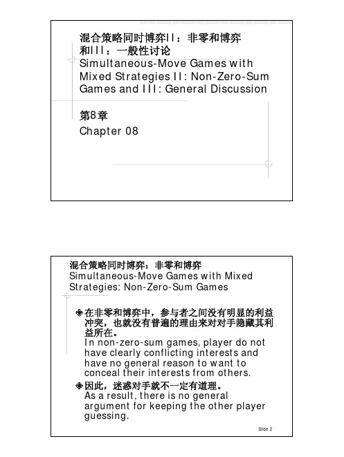
混合策略同时博弈II：非零和博弈 和III：一般性讨论 Simultaneous-Move Games with Mixed Strategies II: Non-Zero-Sum Games and III: General Discussion 第8章 Chapter 08混合策略同时博弈：非零和博弈 Simultaneous-Move Games with Mixed Strategies: Non-Zero-Sum Games 在非零和博弈中，参与者之间没有明显的利益 冲突，也就没有普遍的理由来对对手隐藏其利 益所在。

In non-zero-sum games, player do not have clearly conflicting interests and have no general reason to want to conceal their interests from others. 因此，迷惑对手就不一定有道理。

As a result, there is no general argument for keeping the other player guessing.Slide 2由于不确定的信念导致的混合策略 Mixing Sustained by Uncertain Beliefs不过，由于是同时博弈，参与者可能不得不持 有对对手行动的某种不确定性的信念，因而也 就不能确定地给出自己的最优行动。

However, Simultaneous play can still lead players to have uncertain beliefs about the actions of a rival player and therefore to be uncertain about their own best actions.Slide 3哈里和萨莉能否会面？ Will Harry Meet Sally?SALLY Starbucks Starbucks HARRY Local Latte 0, 0 2, 2 1, 1 Local Latte 0, 0Slide 4哈里和萨莉能否会面？ Will Harry Meet Sally?Sally’s Payoffs2Local LatteSally’s best-response1Starbucks0 2/3Harry’s p-mix1Slide 5哈里和萨莉能否会面？ Will Harry Meet Sally?Sally’s 1 q-mix2/33 Nash EquilibriaHarry’s best response02/3Harry’s p-mixSlide 61Sally’s best response哈里和萨莉能否会面？ Will Harry Meet Sally?混合策略均衡下每个人的期望收益为2/3，小于任何 一个纯策略均衡（2或1）。

zero的隐喻与解释
嘿，你知道吗，zero 这个小小的数字，可有着大大的含义呢！就好像是一片空白的画布，等待着我们去挥洒色彩，创造出独一无二的画作。

比如说，当你开始学习一项新技能的时候，一开始不就像是站在zero 的起点上吗？啥都不懂，啥都不会，但这也正是充满无限可能的时候呀！就像学骑自行车，一开始可能连车都上不去，还摔得七荤八素的，可一旦掌握了技巧，不就能风驰电掣了嘛！
zero 也可以隐喻着重新开始。

人生中总会遇到各种挫折和失败，有时候感觉一切都回到了原点，回到了那个 zero。

但这又怎么样呢？这恰恰是一个新的机会呀！就像游戏里角色挂掉了重新复活在起点，我们可以带着之前的经验教训，再次出发。

“哎呀，失败了又怎样，大不了从零开始呗！”你看，这多带劲。

还有啊，zero 在某些时候还代表着一种纯净和简单。

没有那么多复杂的东西，就是纯粹的零。

就好像我们内心深处的那片宁静之地，没有喧嚣，没有烦恼。

想想看，当你找个安静的角落，闭上眼睛，感受那份 zero 的宁静，是不是特别惬意？
我觉得 zero 就像是生活中的一个神奇密码，它有着各种各样的解释和隐喻。

它可以是起点，可以是重新开始，也可以是纯净简单。

它提
醒着我们，无论处于什么状态，都有着无限的可能和机会。

不要害怕zero，要拥抱它，因为它可能会带你走向意想不到的精彩呢！。

CHAPTER 10: ARBITRAGE PRICING THEORY ANDMULTIFACTOR MODELS OF RISK AND RETURN PROBLEM SETS1. The revised estimate of the expected rate of return on the stock would be the oldestimate plus the sum of the products of the unexpected change in each factor times the respective sensitivity coefficient:Revised estimate = 12% + [(1 × 2%) + (0.5 × 3%)] = 15.5%Note that the IP estimate is computed as: 1 × (5% - 3%), and the IR estimate iscomputed as: 0.5 × (8% - 5%).2. The APT factors must correlate with major sources of uncertainty, i.e., sources ofuncertainty that are of concern to many investors. Researchers should investigatefactors that correlate with uncertainty in consumption and investment opportunities.GDP, the inflation rate, and interest rates are among the factors that can be expected to determine risk premiums. In particular, industrial production (IP) is a goodindicator of changes in the business cycle. Thus, IP is a candidate for a factor that is highly correlated with uncertainties that have to do with investment andconsumption opportunities in the economy.3. Any pattern of returns can be explained if we are free to choose an indefinitelylarge number of explanatory factors. If a theory of asset pricing is to have value, itmust explain returns using a reasonably limited number of explanatory variables(i.e., systematic factors such as unemployment levels, GDP, and oil prices).4. Equation 10.11 applies here:E(r p) = r f + βP1 [E(r1 ) −r f ] + βP2 [E(r2 ) – r f]We need to find the risk premium (RP) for each of the two factors:RP1 = [E(r1 ) −r f] and RP2 = [E(r2 ) −r f]In order to do so, we solve the following system of two equations with two unknowns: .31 = .06 + (1.5 ×RP1 ) + (2.0 ×RP2 ).27 = .06 + (2.2 ×RP1 ) + [(–0.2) ×RP2 ]The solution to this set of equations isRP1 = 10% and RP2 = 5%Thus, the expected return-beta relationship isE(r P) = 6% + (βP1× 10%) + (βP2× 5%)5. The expected return for portfolio F equals the risk-free rate since its beta equals 0.For portfolio A, the ratio of risk premium to beta is (12 − 6)/1.2 = 5For portfolio E, the ratio is lower at (8 – 6)/0.6 = 3.33This implies that an arbitrage opportunity exists. For instance, you can create aportfolio G with beta equal to 0.6 (the same as E’s) by combining portfolio A and portfolio F in equal weights. The expected return and beta for portfolio G are then: E(r G) = (0.5 × 12%) + (0.5 × 6%) = 9%βG = (0.5 × 1.2) + (0.5 × 0%) = 0.6Comparing portfolio G to portfolio E, G has the same beta and higher return.Therefore, an arbitrage opportunity exists by buying portfolio G and selling anequal amount of portfolio E. The profit for this arbitrage will ber G – r E =[9% + (0.6 ×F)] − [8% + (0.6 ×F)] = 1%That is, 1% of the funds (long or short) in each portfolio.6. Substituting the portfolio returns and betas in the expected return-beta relationship,we obtain two equations with two unknowns, the risk-free rate (r f) and the factor risk premium (RP):12% = r f + (1.2 ×RP)9% = r f + (0.8 ×RP)Solving these equations, we obtainr f = 3% and RP = 7.5%7. a. Shorting an equally weighted portfolio of the ten negative-alpha stocks andinvesting the proceeds in an equally-weighted portfolio of the 10 positive-alpha stocks eliminates the market exposure and creates a zero-investmentportfolio. Denoting the systematic market factor as R M, the expected dollarreturn is (noting that the expectation of nonsystematic risk, e, is zero):$1,000,000 × [0.02 + (1.0 ×R M)] − $1,000,000 × [(–0.02) + (1.0 ×R M)]= $1,000,000 × 0.04 = $40,000The sensitivity of the payoff of this portfolio to the market factor is zerobecause the exposures of the positive alpha and negative alpha stocks cancelout. (Notice that the terms involving R M sum to zero.) Thus, the systematiccomponent of total risk is also zero. The variance of the analyst’s profit is notzero, however, since this portfolio is not well diversified.For n = 20 stocks (i.e., long 10 stocks and short 10 stocks) the investor willhave a $100,000 position (either long or short) in each stock. Net marketexposure is zero, but firm-specific risk has not been fully diversified. Thevariance of dollar returns from the positions in the 20 stocks is20 × [(100,000 × 0.30)2] = 18,000,000,000The standard deviation of dollar returns is $134,164.b. If n = 50 stocks (25 stocks long and 25 stocks short), the investor will have a$40,000 position in each stock, and the variance of dollar returns is50 × [(40,000 × 0.30)2] = 7,200,000,000The standard deviation of dollar returns is $84,853.Similarly, if n = 100 stocks (50 stocks long and 50 stocks short), the investorwill have a $20,000 position in each stock, and the variance of dollar returns is100 × [(20,000 × 0.30)2] = 3,600,000,000The standard deviation of dollar returns is $60,000.Notice that, when the number of stocks increases by a factor of 5 (i.e., from 20 to 100), standard deviation decreases by a factor of 5= 2.23607 (from$134,164 to $60,000).8. a. )(σσβσ2222e M +=88125)208.0(σ2222=+×=A50010)200.1(σ2222=+×=B97620)202.1(σ2222=+×=Cb. If there are an infinite number of assets with identical characteristics, then awell-diversified portfolio of each type will have only systematic risk since thenonsystematic risk will approach zero with large n. Each variance is simply β2 × market variance:222Well-diversified σ256Well-diversified σ400Well-diversified σ576A B C;;;The mean will equal that of the individual (identical) stocks.c. There is no arbitrage opportunity because the well-diversified portfolios allplot on the security market line (SML). Because they are fairly priced, there isno arbitrage.9. a. A long position in a portfolio (P) composed of portfolios A and B will offer anexpected return-beta trade-off lying on a straight line between points A and B.Therefore, we can choose weights such that βP = βC but with expected returnhigher than that of portfolio C. Hence, combining P with a short position in Cwill create an arbitrage portfolio with zero investment, zero beta, and positiverate of return.b. The argument in part (a) leads to the proposition that the coefficient of β2must be zero in order to preclude arbitrage opportunities.10. a. E(r) = 6% + (1.2 × 6%) + (0.5 × 8%) + (0.3 × 3%) = 18.1%b.Surprises in the macroeconomic factors will result in surprises in the return ofthe stock:Unexpected return from macro factors =[1.2 × (4% – 5%)] + [0.5 × (6% – 3%)] + [0.3 × (0% – 2%)] = –0.3%E(r) =18.1% − 0.3% = 17.8%11. The APT required (i.e., equilibrium) rate of return on the stock based on r f and thefactor betas isRequired E(r) = 6% + (1 × 6%) + (0.5 × 2%) + (0.75 × 4%) = 16% According to the equation for the return on the stock, the actually expected return on the stock is 15% (because the expected surprises on all factors are zero bydefinition). Because the actually expected return based on risk is less than theequilibrium return, we conclude that the stock is overpriced.12. The first two factors seem promising with respect to the likely impact on the firm’scost of capital. Both are macro factors that would elicit hedging demands acrossbroad sectors of investors. The third factor, while important to Pork Products, is a poor choice for a multifactor SML because the price of hogs is of minor importance to most investors and is therefore highly unlikely to be a priced risk factor. Betterchoices would focus on variables that investors in aggregate might find moreimportant to their welfare. Examples include: inflation uncertainty, short-terminterest-rate risk, energy price risk, or exchange rate risk. The important point here is that, in specifying a multifactor SML, we not confuse risk factors that are important toa particular investor with factors that are important to investors in general; only the latter are likely to command a risk premium in the capital markets.13. The formula is ()0.04 1.250.08 1.50.02.1717%E r =+×+×==14. If 4%f r = and based on the sensitivities to real GDP (0.75) and inflation (1.25),McCracken would calculate the expected return for the Orb Large Cap Fund to be:()0.040.750.08 1.250.02.040.0858.5% above the risk free rate E r =+×+×=+=Therefore, Kwon’s fundamental analysis estimate is congruent with McCracken’sAPT estimate. If we assume that both Kwon and McCracken’s estimates on the return of Orb’s Large Cap Fund are accurate, then no arbitrage profit is possible.15. In order to eliminate inflation, the following three equations must be solvedsimultaneously, where the GDP sensitivity will equal 1 in the first equation,inflation sensitivity will equal 0 in the second equation and the sum of the weights must equal 1 in the third equation.1.1.250.75 1.012.1.5 1.25 2.003.1wx wy wz wz wy wz wx wy wz ++=++=++=Here, x represents Orb’s High Growth Fund, y represents Large Cap Fund and z represents Utility Fund. Using algebraic manipulation will yield wx = wy = 1.6 and wz = -2.2.16. Since retirees living off a steady income would be hurt by inflation, this portfoliowould not be appropriate for them. Retirees would want a portfolio with a return positively correlated with inflation to preserve value, and less correlated with the variable growth of GDP. Thus, Stiles is wrong. McCracken is correct in that supply side macroeconomic policies are generally designed to increase output at aminimum of inflationary pressure. Increased output would mean higher GDP, which in turn would increase returns of a fund positively correlated with GDP.17. The maximum residual variance is tied to the number of securities (n ) in theportfolio because, as we increase the number of securities, we are more likely to encounter securities with larger residual variances. The starting point is todetermine the practical limit on the portfolio residual standard deviation, σ(e P ), that still qualifies as a well-diversified portfolio. A reasonable approach is to compareσ2(e P) to the market variance, or equivalently, to compare σ(e P) to the market standard deviation. Suppose we do not allow σ(e P) to exceed pσM, where p is a small decimal fraction, for example, 0.05; then, the smaller the value we choose for p, the more stringent our criterion for defining how diversified a well-diversified portfolio must be.Now construct a portfolio of n securities with weights w1, w2,…,w n, so that Σw i =1. The portfolio residual variance is σ2(e P) = Σw12σ2(e i)To meet our practical definition of sufficiently diversified, we require this residual variance to be less than (pσM)2. A sure and simple way to proceed is to assume the worst, that is, assume that the residual variance of each security is the highest possible value allowed under the assumptions of the problem: σ2(e i) = nσ2MIn that case σ2(e P) = Σw i2 nσM2Now apply the constraint: Σw i2 nσM2 ≤ (pσM)2This requires that: nΣw i2 ≤ p2Or, equivalently, that: Σw i2 ≤ p2/nA relatively easy way to generate a set of well-diversified portfolios is to use portfolio weights that follow a geometric progression, since the computations then become relatively straightforward. Choose w1 and a common factor q for the geometric progression such that q < 1. Therefore, the weight on each stock is a fraction q of the weight on the previous stock in the series. Then the sum of n terms is:Σw i= w1(1– q n)/(1– q) = 1or: w1 = (1– q)/(1– q n)The sum of the n squared weights is similarly obtained from w12 and a common geometric progression factor of q2. ThereforeΣw i2 = w12(1– q2n)/(1– q 2)Substituting for w1 from above, we obtainΣw i2 = [(1– q)2/(1– q n)2] × [(1– q2n)/(1– q 2)]For sufficient diversification, we choose q so that Σw i2 ≤ p2/nFor example, continue to assume that p = 0.05 and n = 1,000. If we chooseq = 0.9973, then we will satisfy the required condition. At this value for q w1 = 0.0029 and w n = 0.0029 × 0.99731,000In this case, w1 is about 15 times w n. Despite this significant departure from equal weighting, this portfolio is nevertheless well diversified. Any value of q between0.9973 and 1.0 results in a well-diversified portfolio. As q gets closer to 1, theportfolio approaches equal weighting.18. a. Assume a single-factor economy, with a factor risk premium E M and a (large)set of well-diversified portfolios with beta βP. Suppose we create a portfolio Zby allocating the portion w to portfolio P and (1 – w) to the market portfolioM. The rate of return on portfolio Z is:R Z = (w × R P) + [(1 – w) × R M]Portfolio Z is riskless if we choose w so that βZ = 0. This requires that:βZ = (w × βP) + [(1 – w) × 1] = 0 ⇒w = 1/(1 – βP) and (1 – w) = –βP/(1 – βP)Substitute this value for w in the expression for R Z:R Z = {[1/(1 – βP)] × R P} – {[βP/(1 – βP)] × R M}Since βZ = 0, then, in order to avoid arbitrage, R Z must be zero.This implies that: R P = βP × R MTaking expectations we have:E P = βP × E MThis is the SML for well-diversified portfolios.b. The same argument can be used to show that, in a three-factor model withfactor risk premiums E M, E1 and E2, in order to avoid arbitrage, we must have:E P = (βPM × E M) + (βP1 × E1) + (βP2 × E2)This is the SML for a three-factor economy.19. a. The Fama-French (FF) three-factor model holds that one of the factors drivingreturns is firm size. An index with returns highly correlated with firm size (i.e.,firm capitalization) that captures this factor is SMB (small minus big), thereturn for a portfolio of small stocks in excess of the return for a portfolio oflarge stocks. The returns for a small firm will be positively correlated withSMB. Moreover, the smaller the firm, the greater its residual from the othertwo factors, the market portfolio and the HML portfolio, which is the returnfor a portfolio of high book-to-market stocks in excess of the return for aportfolio of low book-to-market stocks. Hence, the ratio of the variance of thisresidual to the variance of the return on SMB will be larger and, together withthe higher correlation, results in a high beta on the SMB factor.b.This question appears to point to a flaw in the FF model. The model predictsthat firm size affects average returns so that, if two firms merge into a largerfirm, then the FF model predicts lower average returns for the merged firm.However, there seems to be no reason for the merged firm to underperformthe returns of the component companies, assuming that the component firmswere unrelated and that they will now be operated independently. We mighttherefore expect that the performance of the merged firm would be the sameas the performance of a portfolio of the originally independent firms, but theFF model predicts that the increased firm size will result in lower averagereturns. Therefore, the question revolves around the behavior of returns for aportfolio of small firms, compared to the return for larger firms that resultfrom merging those small firms into larger ones. Had past mergers of smallfirms into larger firms resulted, on average, in no change in the resultantlarger firms’ stock return characteristics (compared to the portfolio of stocksof the merged firms), the size factor in the FF model would have failed.Perhaps the reason the size factor seems to help explain stock returns is that,when small firms become large, the characteristics of their fortunes (andhence their stock returns) change in a significant way. Put differently, stocksof large firms that result from a merger of smaller firms appear empirically tobehave differently from portfolios of the smaller component firms.Specifically, the FF model predicts that the large firm will have a smaller riskpremium. Notice that this development is not necessarily a bad thing for thestockholders of the smaller firms that merge. The lower risk premium may bedue, in part, to the increase in value of the larger firm relative to the mergedfirms.CFA PROBLEMS1. a. This statement is incorrect. The CAPM requires a mean-variance efficientmarket portfolio, but APT does not.b.This statement is incorrect. The CAPM assumes normally distributed securityreturns, but APT does not.c. This statement is correct.2. b. Since portfolio X has β = 1.0, then X is the market portfolio and E(R M) =16%.Using E(R M ) = 16% and r f = 8%, the expected return for portfolio Y is notconsistent.3. d.4. c.5. d.6. c. Investors will take on as large a position as possible only if the mispricingopportunity is an arbitrage. Otherwise, considerations of risk anddiversification will limit the position they attempt to take in the mispricedsecurity.7. d.8. d.。

layuitable表格分页从0开始，⾃定义请求参数
最近⽤layui的时候发现⼀个很严重的问题。

写demo的时候发现分页是从第1页开始，不是从第0页开始，但是后台固定了摸得改。

发现官⽅暂时没有发现什么有效的操作⼿段，于是乎，⾃⼰动⼿，丰⾐⾜⾷。

//修改版本2.5.4
//现在是第⼆版，第⼀版有BUG T_T
https:///s/1aL-E_R9_vby_EtqBSqa9-Q
tjf1
把这两个⽂件复制到layui 的 modules 下覆盖它，然后在table 渲染的时候加上这个属性。

如果是0则从第0页开始，如果是1，从第⼀页开始（原先的设想是设置成N从第N开始，但是失败了~~~~~）
修改完成后，分页从第0也开始了。

哇哈哈哈哈
修改的逻辑就是发送分页请求的时候如果startByZero是0，请求的参数减⼀，分页的时候如果分页是0，就当1处理，其他照旧。

改这种转化后的的代码也是⽐较蠢的，如果有童鞋有更好的⽅式，请联系⼀下我啦，谢谢。

————————————————————————————————————————————————
//2019-8-21
//版本2.5.4
修改startByZero 属性为true和false，修复序号显⽰BUG
添加pageObject 属性，添加后可以在请求的分页JSON请求上再添加⼀个⽗节点⽐如这样：这⾥pageObject 填写是rsf。

Chapter 08Index Models Multiple Choice Questions1. As diversification increases, the total variance of a portfolio approaches ____________.A. 0B. 1C. the variance of the market portfolioD. infinityE. −12. As diversification increases, the standard deviation of a portfolio approaches____________.A. 0B. 1C. infinityD. the standard deviation of the market portfolioE. −13. As diversification increases, the firm-specific risk of a portfolio approaches ____________.A. 0B. 1C. infinityD. n−1 * nE. −14. As diversification increases, the unsystematic risk of a portfolio approaches ____________.A. 1B. 0C. infinityD. n−1 * nE. −15. As diversification increases, the unique risk of a portfolio approaches ____________.A. 1B. 0C. infinityD. n−1 * nE. −16. The index model was first suggested by ____________.A. GrahamB. MarkowitzC. MillerD. SharpeE. Jensen7. A single-index model uses __________ as a proxy for the systematic risk factor.A. a market index, such as the S&P 500B. the current account deficitC. the growth rate in GNPD. the unemployment rateE. the inflation rate8. Beta books typically rely on the __________ most recent monthly observations to calculate regression parameters.A. 12B. 36C. 60D. 120E. 69. The index model has been estimated for stocks A and B with the following results:R A= 0.03 + 0.7R M+ e AR B= 0.01 + 0.9R M+ e BσM= 0.35 σ(e A) = 0.20 σ(e B) = 0.10The covariance between the returns on stocks A and B is ___________.A. 0.0384B. 0.0406C. 0.1920D. 0.0772E. 0.400010. According to the index model, covariances among security pairs areA. due to the influence of a single common factor represented by the market index return.B. extremely difficult to calculate.C. related to industry-specific events.D. usually positive.E. due to the influence of a single common factor represented by the market index return, and they are usually positive.11. The intercept in the regression equations calculated by beta books is equal toA. α in the CAPM.B. α + rf(1 + β).C. α + rf(1 −β).D. 1 −α.E. 1.12. Analysts may use regression analysis to estimate the index model for a stock. When doing so, the slope of the regression line is an estimate of ______________.A. the α of the assetB. the β of the assetC. the σ of the assetD. the δ of the assetE. the ρ of the asset13. Analysts may use regression analysis to estimate the index model for a stock. When doing so, the intercept of the regression line is an estimate of ______________.A. the α of the assetB. the β of the assetC. the σ of the assetD. the δ of the assetE. the ρ of the asset14. In a factor model, the return on a stock in a particular period will be related to _________.A. firm-specific eventsB. macroeconomic eventsC. the error termD. both firm-specific events and macroeconomic eventsE. neither firm-specific events nor macroeconomic events15. Rosenberg and Guy found that __________ helped to predict a firm's beta.A. the firm's financial characteristicsB. the firm's industry groupC. firm sizeD. both the firm's financial characteristics and the firm's industry groupE. the firm's financial characteristics, the firm's industry group and firm size16. If the index model is valid, _________ would be helpful in determining the covariance between assets GM and GE.A. βGMB. βGEC. σMD. βGM, βGE, and σME. βGE, and σM17. If the index model is valid, _________ would be helpful in determining the covariance between assets HPQ and KMP.A. βHPQB. βKMPC. σMD. βHPQ,βKMP, andσME. βHPQ, andβKMP18. If the index model is valid, _________ would be helpful in determining the covariance between assets K and L.A. βkB. βLC. σMD. βk,βL, andσME. βk, andβL19. Rosenberg and Guy found that ___________ helped to predict firms' betas.A. debt/asset ratiosB. market capitalizationC. variance of earningsD. debt/asset ratios, market capitalization, and variance of earningsE. debt/asset ratios and variance of earnings only20. If a firm's beta was calculated as 0.6 in a regression equation, a commonly used adjustment technique would provide an adjusted beta ofA. less than 0.6 but greater than zero.B. between 0.6 and 1.0.C. between 1.0 and 1.6.D. greater than 1.6.E. zero or less.21. If a firm's beta was calculated as 0.8 in a regression equation, a commonly used adjustment technique would provide an adjusted beta ofA. less than 0.8 but greater than zero.B. between 1.0 and 1.8.C. between 0.8 and 1.0.D. greater than 1.8.E. zero or less.22. If a firm's beta was calculated as 1.3 in a regression equation, a commonly used adjustment technique would provide an adjusted beta ofA. less than 1.0 but greater than zero.B. between 0.3 and 0.9.C. between 1.0 and 1.3.D. greater than 1.3.E. zero or less.23. The beta of Exxon stock has been estimated as 1.6 using regression analysis on a sample of historical returns. A commonly used adjustment technique would provide an adjusted beta of ___________.A. 1.20B. 1.32C. 1.13D. 1.40E. 1.6524. The beta of Apple stock has been estimated as 2.3 using regression analysis on a sample of historical returns. A commonly used adjustment technique would provide an adjusted beta of ___________.A. 2.20B. 1.87C. 2.13D. 1.66E. 1.9325. The beta of JCP stock has been estimated as 1.2 using regression analysis on a sample of historical returns. A commonly used adjustment technique would provide an adjusted beta of ___________.A. 1.20B. 1.32C. 1.13D. 1.0E. 1.2326. Assume that stock market returns do not resemble a single-index structure. An investment fund analyzes 150 stocks in order to construct a mean-variance efficient portfolio constrained by 150 investments. They will need to calculate _____________ expected returns and___________ variances of returns.A. 150; 150B. 150; 22500C. 22500; 150D. 22500; 22500E. 300; 30027. Assume that stock market returns do not resemble a single-index structure. An investment fund analyzes 100 stocks in order to construct a mean-variance efficient portfolio constrained by 100 investments. They will need to calculate _____________ expected returns and___________ variances of returns.A. 100; 100B. 100; 4950C. 4950; 100D. 4950; 4950E. 200; 20028. Assume that stock market returns do not resemble a single-index structure. An investment fund analyzes 150 stocks in order to construct a mean-variance efficient portfolio constrained by 150 investments. They will need to calculate ____________ covariances.A. 12B. 150C. 22,500D. 11,175E. 30029. Assume that stock market returns do not resemble a single-index structure. An investment fund analyzes 125 stocks in order to construct a mean-variance efficient portfolio constrained by 125 investments. They will need to calculate ____________ covariances.A. 125B. 7,750C. 15,625D. 11,750E. 25030. Assume that stock market returns do not resemble a single-index structure. An investment fund analyzes 100 stocks in order to construct a mean-variance efficient portfolio constrained by 100 investments. They will need to calculate ____________ covariances.A. 45B. 100C. 4,950D. 10,000E. 20031. Assume that stock market returns do follow a single-index structure. An investment fund analyzes 175 stocks in order to construct a mean-variance efficient portfolio constrained by 175 investments. They will need to calculate ________ estimates of expected returns and ________ estimates of sensitivity coefficients to the macroeconomic factor.A. 175; 15,225B. 175; 175C. 15,225; 175D. 15,225; 15,225E. 350; 35032. Assume that stock market returns do follow a single-index structure. An investment fund analyzes 125 stocks in order to construct a mean-variance efficient portfolio constrained by 125 investments. They will need to calculate ________ estimates of expected returns and ________ estimates of sensitivity coefficients to the macroeconomic factor.A. 125; 15,225B. 15,625; 125C. 7,750; 125D. 125; 125E. 250; 25033. Assume that stock market returns do follow a single-index structure. An investment fund analyzes 200 stocks in order to construct a mean-variance efficient portfolio constrained by 200 investments. They will need to calculate ________ estimates of expected returns and ________ estimates of sensitivity coefficients to the macroeconomic factor.A. 200; 19,900B. 200; 200C. 19,900; 200D. 19,900; 19.900E. 400; 40034. Assume that stock market returns do follow a single-index structure. An investment fund analyzes 500 stocks in order to construct a mean-variance efficient portfolio constrained by 500 investments. They will need to calculate ________ estimates of firm-specific variances and________ estimate/estimates for the variance of the macroeconomic factor.A. 500; 1B. 500; 500C. 124,750; 1D. 124,750; 500E. 250,000; 50035. Consider the single-index model. The alpha of a stock is 0%. The return on the market index is 16%. The risk-free rate of return is 5%. The stock earns a return that exceeds the risk-free rate by 11% and there are no firm-specific events affecting the stock performance. The β of the stock is _______.A. 0.67B. 0.75C. 1.0D. 1.33E. 1.5036. Suppose you held a well-diversified portfolio with a very large number of securities, and that the single index model holds. If the σ of your portfolio was 0.20 and σM was 0.16, the β of the portfolio would be approximately ________.A. 0.64B. 0.80C. 1.25D. 1.56E. 1.4237. Suppose you held a well-diversified portfolio with a very large number of securities, and that the single index model holds. If the σ of your portfolio was 0.22 and σM was 0.19, the β of the portfolio would be approximately ________.A. 1.34B. 1.16C. 1.25D. 1.56E. 1.2138. Suppose you held a well-diversified portfolio with a very large number of securities, and that the single index model holds. If the σ of your portfolio was 0.18 and σM was 0.24, the β of the portfolio would be approximately ________.A. 0.75B. 0.56C. 0.07D. 1.03E. 0.8639. Suppose the following equation best describes the evolution of β over time:βt= 0.25 + 0.75βt-1If a stock had a β of 0.6 last year, you would forecast the β to be _______ in the coming year.A. 0.45B. 0.60C. 0.70D. 0.75E. 0.5540. Suppose the following equation best describes the evolution of β over time:βt= 0.31 + 0.82βt-1If a stock had a β of 0.88 last year, you would forecast the β to be _______ in the coming year.A. 0.88B. 0.82C. 0.31D. 1.03E. 1.1241. Suppose the following equation best describes the evolution of β over time:βt= 0.18 + 0.63βt-1If a stock had a β of 1.09 last year, you would forecast the β to be _______ in the coming year.A. 0.87B. 0.18C. 0.63D. 0.81E. 0.9642. An analyst estimates the index model for a stock using regression analysis involving total returns. The estimated the intercept in the regression equation is 6% and the β is 0.5. Therisk-free rate of return is 12%. The true β of the stock is ________.A. 0%B. 3%C. 6%D. 9%E. −1%43. The index model for stock A has been estimated with the following result:R A= 0.01 + 0.9R M+ e AIf σM= 0.25 and R2A= 0.25, the standard deviation of return of stock A is _________.A. 0.2025B. 0.2500C. 0.4500D. 0.8100E. 0.546044. The index model for stock B has been estimated with the following result:R B= 0.01 + 1.1R M+ e BIf σM= 0.20 and R2B= 0.50, the standard deviation of the return on stock B is _________.A. 0.1111B. 0.2111C. 0.3111D. 0.4111E. 0.131145. Suppose you forecast that the market index will earn a return of 15% in the coming year. Treasury bills are yielding 6%. The unadjusted β of Mobil stock is 1.30. A reasonable forecast of the return on Mobil stock for the coming year is _________ if you use a common method to derive adjusted betas.A. 15.0%B. 15.5%C. 16.0%D. 16.8%E. 17.4%46. The index model has been estimated for stocks A and B with the following results: R A= 0.01 + 0.5R M+ e AR B= 0.02 + 1.3R M+ e BσM= 0.25 σ(e A) = 0.20 σ(e B) = 0.10The covariance between the returns on stocks A and B is ___________.A. 0.0384B. 0.0406C. 0.1920D. 0.0050E. 0.400047. The index model has been estimated for stocks A and B with the following results: R A= 0.01 + 0.8R M+ e AR B= 0.02 + 1.2R M+ e BσM= 0.20 σ(e A) = 0.20 σ (e B) = 0.10The standard deviation for stock A is __________.A. 0.0656B. 0.0676C. 0.2561D. 0.2600E. 0.356448. The index model has been estimated for stock A with the following results:R A= 0.01 + 0.8R M+ e AσM= 0.20 σ(e A) = 0.10The standard deviation of the return for stock A is __________.A. 0.0356B. 0.1886C. 0.1600D. 0.6400E. 0.215349. Security returnsA. are based on both macro events and firm-specific events.B. are based on firm-specific events only.C. are usually positively correlated with each other.D. are based on both macro events and firm-specific events and are usually negatively correlated with each other.E. are based on both macro events and firm-specific events and are usually positively correlated with each other.50. The single-index modelA. greatly reduces the number of required calculations, relative to those required by the Markowitz model.B. enhances the understanding of systematic versus nonsystematic risk.C. greatly increases the number of required calculations, relative to those required by the Markowitz model.D. greatly reduces the number of required calculations, relative to those required by the Markowitz model and enhances the understanding of systematic versus nonsystematic risk.E. enhances the understanding of systematic versus nonsystematic risk and greatly increases the number of required calculations, relative to those required by the Markowitz model.51. The Security Characteristic Line (SCL)A. plots the excess return on a security as a function of the excess return on the market.B. allows one to estimate the beta of the security.C. allows one to estimate the alpha of the security.D. plots the excess return on a security as a function of the excess return on the market, allows one to estimate the beta of the security, and allows one to estimate the alpha of the security.E. allows one to estimate the gamma of the security.52. The expected impact of unanticipated macroeconomic events on a security's return during the period isA. included in the security's expected return.B. zero.C. equal to the risk free rate.D. proportional to the firm's beta.E. infinite.53. Covariances between security returns tend to beA. positive because of SEC regulations.B. positive because of Exchange regulations.C. positive because of economic forces that affect many firms.D. negative because of SEC regulations.E. negative because of economic forces that affect many firms.54. In the single-index model represented by the equation r i = E(r i) + i F + e i, the term e i representsA. the impact of unanticipated macroeconomic events on security i's return.B. the impact of unanticipated firm-specific events on security i's return.C. the impact of anticipated macroeconomic events on security i's return.D. the impact of anticipated firm-specific events on security i's return.E. the impact of changes in the market on security i's return.55. Suppose you are doing a portfolio analysis that includes all of the stocks on the NYSE. Using a single-index model rather than the Markowitz model _______ the number of inputs needed from _______ to ________.A. increases; about 1,400; more than 1.4 millionB. increases; about 10,000; more than 125,000C. reduces; more than 125,000; about 10,000D. reduces; more than 4 million; about 9,000E. increases; about 150; more than 1,50056. One "cost" of the single-index model is that itA. is virtually impossible to apply.B. prohibits specialization of efforts within the security analysis industry.C. requires forecasts of the money supply.D. is legally prohibited by the SEC.E. allows for only two kinds of risk—macro risk and micro risk.57. The Security Characteristic Line (SCL) associated with the single-index model is a plot ofA. the security's returns on the vertical axis and the market index's returns on the horizontal axis.B. the market index's returns on the vertical axis and the security's returns on the horizontal axis.C. the security's excess returns on the vertical axis and the market index's excess returns on the horizontal axis.D. the market index's excess returns on the vertical axis and the security's excess returns on the horizontal axis.E. the security's returns on the vertical axis and Beta on the horizontal axis.58. The idea that there is a limit to the reduction of portfolio risk due to diversification isA. contradicted by both the CAPM and the single-index model.B. contradicted by the CAPM.C. contradicted by the single-index model.D. supported in theory, but not supported empirically.E. supported both in theory and by empirical evidence.59. In their study about predicting beta coefficients, which of the following did Rosenberg and Guy find to be factors that influence beta?I) Industry groupII) Variance of cash flowIII) Dividend yieldIV) Growth in earnings per shareA. I and IIB. I and IIIC. I, II, and IIID. I, II, and IVE. I, II, III, and IV60. If a firm's beta was calculated as 1.6 in a regression equation, a commonly used adjustment technique would provide an adjusted beta ofA. less than 0.6 but greater than zero.B. between 0.6 and 1.0.C. between 1.0 and 1.6.D. greater than 1.6.E. zero or less.61. The beta of a stock has been estimated as 1.8 using regression analysis on a sample of historical returns. A commonly used adjustment technique would provide an adjusted beta of ___________.A. 1.20B. 1.53C. 1.13D. 1.0E. 1.7662. Assume that stock market returns do not resemble a single-index structure. An investment fund analyzes 40 stocks in order to construct a mean-variance efficient portfolio constrained by 40 investments. They will need to calculate _____________ expected returns and___________ variances of returns.A. 100; 100B. 40; 40C. 4950; 100D. 4950; 4950E. 80; 8063. Assume that stock market returns do not resemble a single-index structure. An investment fund analyzes 40 stocks in order to construct a mean-variance efficient portfolio constrained by40 investments. They will need to calculate ____________ covariances.A. 45B. 780C. 4,950D. 10,000E. 8064. Assume that stock market returns do follow a single-index structure. An investment fund analyzes 60 stocks in order to construct a mean-variance efficient portfolio constrained by 60 investments. They will need to calculate ________ estimates of expected returns and ________ estimates of sensitivity coefficients to the macroeconomic factor.A. 200; 19,900B. 200; 200C. 60; 60D. 19,900; 19.900E. 120; 12065. Consider the single-index model. The alpha of a stock is 0%. The return on the market index is 10%. The risk-free rate of return is 3%. The stock earns a return that exceeds the risk-free rate by 11% and there are no firm-specific events affecting the stock performance. The β of the stock is _______.A. 0.64B. 0.75C. 1.17D. 1.33E. 1.5066. Suppose you held a well-diversified portfolio with a very large number of securities, and that the single index model holds. If the σ of your portfolio was 0.25 and σM was 0.21, the β of the portfolio would be approximately ________.A. 0.64B. 1.19C. 1.25D. 1.56E. 0.8767. Suppose you held a well-diversified portfolio with a very large number of securities, and that the single index model holds. If the σ of your portfolio was 0.18 and σM was 0.22, the β of the portfolio would be approximately ________.A. 0.64B. 1.19C. 0.82D. 1.56E. 0.9968. Suppose the following equation best describes the evolution of β over time:βt= 0.4 + 0.6βt-1If a stock had a β of 0.9 last year, you would forecast the β to be _______ in the coming year.A. 0.45B. 0.60C. 0.70D. 0.94E. 1.0269. Suppose the following equation best describes the evolution of β over time:βt= 0.3 + 0.2βt-1If a stock had a β of 0.8 last year, you would forecast the β to be _______ in the coming year.A. 0.46B. 0.60C. 0.70D. 0.94E. 0.3770. The index model for stock A has been estimated with the following result:R A= 0.01 + 0.94R M+ e AIf σM= 0.30 and R2A= 0.28, the standard deviation of return of stock A is _________.A. 0.2025B. 0.2500C. 0.4500D. 0.5329E. 0.667171. Suppose you forecast that the market index will earn a return of 12% in the coming year. Treasury bills are yielding 4%. The unadjusted β of Mobil stock is 1.30. A reasonable forecast of the return on Mobil stock for the coming year is _________ if you use a common method to derive adjusted betas.A. 15.0%B. 15.5%C. 16.0%D. 14.6%E. 13.2%72. The index model has been estimated for stocks A and B with the following results:R A= 0.01 + 0.8R M+ e AR B= 0.02 + 1.1R M+ e BσM= 0.30 σ (e A) = 0.20 σ (e B) = 0.10The covariance between the returns on stocks A and B is ___________.A. 0.0384B. 0.0406C. 0.1920D. 0.0050E. 0.079273. If a firm's beta was calculated as 1.35 in a regression equation, a commonly used adjustment technique would provide an adjusted beta of.SSSA. less than 1.35.B. between 0.0 and 1.0.C. between 1.0 and 1.35.D. greater than 1.35.E. zero or less.74. The beta of a stock has been estimated as 1.4 using regression analysis on a sample of historical returns. A commonly used adjustment technique would provide an adjusted beta of ___________.A. 1.27B. 1.32C. 1.13D. 1.0E. 1.4575. The beta of a stock has been estimated as 0.85 using regression analysis on a sample of historical returns. A commonly used adjustment technique would provide an adjusted beta of ___________.A. 1.01B. 0.95C. 1.13D. 0.90E. 0.8876. Assume that stock market returns do not resemble a single-index structure. An investment fund analyzes 125 stocks in order to construct a mean-variance efficient portfolio constrained by 125 investments. They will need to calculate _____________ expected returns and___________ variances of returns.A. 125; 125B. 125; 15,625C. 15,625; 125D. 15,625; 15,625E. 250; 25077. Assume that stock market returns do not resemble a single-index structure. An investment fund analyzes 125 stocks in order to construct a mean-variance efficient portfolio constrained by 125 investments. They will need to calculate ____________ covariances.A. 90B. 125C. 7,750D. 15,625E. 25078. Assume that stock market returns do not resemble a single-index structure. An investment fund analyzes 132 stocks in order to construct a mean-variance efficient portfolio constrained by 132 investments. They will need to calculate ____________ covariances.A. 100B. 132C. 4,950D. 8,646E. 26479. Assume that stock market returns do follow a single-index structure. An investment fund analyzes 217 stocks in order to construct a mean-variance efficient portfolio constrained by 217 investments. They will need to calculate ________ estimates of expected returns and ________ estimates of sensitivity coefficients to the macroeconomic factor.A. 217; 47,089B. 217; 217C. 47,089; 217D. 47,089; 47,089E. 434; 43480. Assume that stock market returns do follow a single-index structure. An investment fund analyzes 750 stocks in order to construct a mean-variance efficient portfolio constrained by 750 investments. They will need to calculate ________ estimates of firm-specific variances and________ estimate/estimates for the variance of the macroeconomic factor.A. 750; 1B. 750; 750C. 124,750; 1D. 124,750; 750E. 562,500; 75081. Consider the single-index model. The alpha of a stock is 0%. The return on the market index is 10%. The risk-free rate of return is 5%. The stock earns a return that exceeds the risk-free rate by 5% and there are no firm-specific events affecting the stock performance. The β of the stock is _______.A. 0.67B. 0.75C. 1.0D. 1.33E. 1.5082. Suppose you held a well-diversified portfolio with a very large number of securities, and that the single index model holds. If the σ of your portfolio was 0.24 and σM was 0.18, the β of the portfolio would be approximately ________.A. 0.64B. 1.33C. 1.25D. 1.56E. 1.4183. Suppose you held a well-diversified portfolio with a very large number of securities, and that the single index model holds. If the σ of your portfolio was 0.14 and σM was 0.19, the β of the portfolio would be approximately ________.A. 0.74B. 0.80C. 1.25D. 1.56E. 0.6484. Suppose the following equation best describes the evolution of β over time:βt= 0.30 + 0.70βt-1If a stock had a β of 0.82 last year, you would forecast the β to be _______ in the coming year.A. 0.91B. 0.77C. 0.63D. 0.87E. 0.95Short Answer Questions85. Discuss the advantages of the single-index model over the Markowitz model in terms of numbers of variable estimates required and in terms of understanding risk relationships.86. Discuss the security characteristic line (SCL).87. Discuss a commonly used adjustment technique to provide an adjusted beta.Chapter 08 Index Models Answer KeyMultiple Choice Questions1. As diversification increases, the total variance of a portfolio approaches ____________.A. 0B. 1C. the variance of the market portfolioD. infinityE. -1As more and more securities are added to the portfolio; unsystematic risk decreases and most of the remaining risk is systematic; as measured by the variance of the market portfolio.AACSB: AnalyticBloom's: UnderstandDifficulty: BasicTopic: Index models2. As diversification increases, the standard deviation of a portfolio approaches____________.A. 0B. 1C. infinityD. the standard deviation of the market portfolioE. -1As more and more securities are added to the portfolio; unsystematic risk decreases and most of the remaining risk is systematic, as measured by the variance (or standard deviation) of the market portfolio.AACSB: AnalyticBloom's: UnderstandDifficulty: BasicTopic: Index models3. As diversification increases, the firm-specific risk of a portfolio approaches ____________.A. 0B. 1C. infinityD. n-1 * nE. -1As more and more securities are added to the portfolio; unsystematic risk decreases and most of the remaining risk is systematic; as measured by the variance (or standard deviation) of the market portfolio.AACSB: AnalyticBloom's: UnderstandDifficulty: BasicTopic: Index models4. As diversification increases, the unsystematic risk of a portfolio approaches ____________.A. 1B. 0C. infinityD. n-1 * nE. -1As more and more securities are added to the portfolio, unsystematic risk decreases and most of the remaining risk is systematic, as measured by the variance (or standard deviation) of the market portfolio.AACSB: AnalyticBloom's: UnderstandDifficulty: BasicTopic: Index models。