OFDM基础中英文对照外文翻译文献
- 格式:doc
- 大小:112.00 KB
- 文档页数:13
外⽂参考⽂献翻译-中⽂基于4G LTE技术的⾼速铁路移动通信系统KS Solanki教授,Kratika ChouhanUjjain⼯程学院,印度Madhya Pradesh的Ujjain摘要:随着时间发展,⾼速铁路(HSR)要求可靠的,安全的列车运⾏和乘客通信。
为了实现这个⽬标,HSR的系统需要更⾼的带宽和更短的响应时间,⽽且HSR的旧技术需要进⾏发展,开发新技术,改进现有的架构和控制成本。
为了满⾜这⼀要求,HSR采⽤了GSM的演进GSM-R技术,但它并不能满⾜客户的需求。
因此采⽤了新技术LTE-R,它提供了更⾼的带宽,并且在⾼速下提供了更⾼的客户满意度。
本⽂介绍了LTE-R,给出GSM-R与LTE-R之间的⽐较结果,并描述了在⾼速下哪种铁路移动通信系统更好。
关键词:⾼速铁路,LTE,GSM,通信和信令系统⼀介绍⾼速铁路需要提⾼对移动通信系统的要求。
随着这种改进,其⽹络架构和硬件设备必须适应⾼达500公⾥/⼩时的列车速度。
HSR还需要快速切换功能。
因此,为了解决这些问题,HSR 需要⼀种名为LTE-R的新技术,基于LTE-R的HSR提供⾼数据传输速率,更⾼带宽和低延迟。
LTE-R能够处理⽇益增长的业务量,确保乘客安全并提供实时多媒体信息。
随着列车速度的不断提⾼,可靠的宽带通信系统对于⾼铁移动通信⾄关重要。
HSR的应⽤服务质量(QOS)测量,包括如数据速率,误码率(BER)和传输延迟。
为了实现HSR的运营需求,需要⼀个能够与 LTE保持⼀致的能⼒的新系统,提供新的业务,但仍能够与GSM-R长时间共存。
HSR系统选择合适的⽆线通信系统时,需要考虑性能,服务,属性,频段和⼯业⽀持等问题。
4G LTE系统与第三代(3G)系统相⽐,它具有简单的扁平架构,⾼数据速率和低延迟。
在LTE的性能和成熟度⽔平上,LTE- railway(LTE-R)将可能成为下⼀代HSR通信系统。
⼆ LTE-R系统描述考虑LTE-R的频率和频谱使⽤,对为⾼速铁路(HSR)通信提供更⾼效的数据传输⾮常重要。
附录一、英文原文OFDM Channel Estimation in the Presence of Frequency Offset andPhase NoiseAbstract–In this paper, we consider OFDM channel estimation in the presence of frequency offset and phase noise. In the literatures, most channel estimation methods assume perfect frequency synchronization and the knowledge of channel statistics. Phase noise and residual frequency offset cause inter-carrier interference (ICI), which consequently impairs the accuracy of channel estimation. The lack of knowledge of channel statistics can make channel estimation much harder. To resolve these problems, we propose with the aid of cyclic prefix (CP) based frequency offset estimation statistics-independent channel estimation. We iteratively search for the most likely channel impulse response (CIR) length, and use it not only for the optimum compensation of frequency offset, but also for finding the optimum window to filter the least square (LS) channel estimate which further suppress the effects of ICI and noise. The proposed scheme is compared with conventional methods for both non-interpolation and interpolation cases2. Numerical results are presented to illustrate the effectiveness of the proposed scheme.I. INTRODUCTIONOrthogonal frequency division multiplexing (OFDM) is a bandwidth efficient transmission technique which provides high bandwidth efficiency and is quite effective in handling time dispersion of multipath fading channels. It has been chosen as the transmission method of many standards in wire and wireless communications, such as Digital Subscribe Line (DSL), European Digital Audio and Video Broadcasting (DAB/DVB), IEEE 802.11a and European HIPERLAN/2 for wireless local area network (WLAN) etc..Based on multi-carrier modulation [1], OFDM has symbol period long enough to eliminate inter-symbol interference (ISI) caused by time dispersive channels. Nevertheless, the multicarrier modulation is also sensitive to frequency offset and phase noise. Frequency offset and phase noise cause loss of orthogonality among subcarriers and consequently introduce inter-carrier interference (ICI). The effect of phase noise has been analyzed in many papers [2]-[4]. Many approaches have also been proposed to analyze, estimate and compensate frequency offset [2][5]-[10]. Though it is impossible to estimate random phase noise, frequency offset estimation can be achieved by using pilot signals [5][6]. As these methods cause loss of bandwidth efficiency, non-pilot-aided frequency offset estimation has be used [7]-[10]. The cyclic prefix (CP) based method, initially proposed in [9], is quite attractive among non-pilot-aided approaches due to its simplicity. Nevertheless, the accuracy of the CP-based method could not be guaranteed for multipath fading channels. Later, asproposed in [10], the method of [9] was improved by considering the channel impulse response (CIR) length. The proposed method in [10], however, is not feasible in cases when the CIR length is unknown.Furthermore, channel estimation is a very important issue for OFDM systems. Blind channel estimation is a desirable approach as it does not require pilot signals. It does require, however, a large amount of data and thus higher computational complexity. With perfect frequency synchronization (without residual frequency offset), different pilot-symbol-aided channel estimation methods can be applied in OFDM [11]-[14]. The maximum likelihood/least square (ML/LS) estimators of [11] and [12] can readily be implemented without knowing channel statistics. The minimum mean square error (MMSE) estimators in [12]-[14], however, are more robust against noise and perform better than the ML/LS estimators. Nevertheless, its dependence on channel statistics and the operating signal to noise ratio (SNR) makes it disadvantageous. Despite its robustness against mismatch [13][14], when there is no a priori knowledge of channel statistics and the operating SNR, the performance inevitably degrades. Without the assumption of perfect frequency synchronization, the performance may further degrade due to frequency offset and phase noise.In this paper, we consider statistics-independent channel estimation in the presence of frequency offset and phase noise. As a function of the CIR length, the LS channel estimate results, which is based on the CP-based frequency offset estimation and compensation, are used to search for the CIR length iteratively. The minimization of channel estimation errors leads to the most likely CIR length, which is then used to optimize frequency offset estimate, and filter the LS channel estimate reducing its sensitivity to noise and ICI. Thus better performance is achieved.The paper is organized as follows. The OFDM system model is introduced in Section II. Section III presents and analyzes the proposed frequency offset and channel estimation scheme. Section IV provides the numerical results to illustrate the effectiveness of the proposed scheme. The paper is concluded in Section V.II. OFDM SYSTEM MODELThe basic principle of OFDM is to divide each data symbol into N samples (subcarriers). The length N discrete Fourier transform (DFT) is applied to those samples and a cyclic prefix(CP) is added to eliminate ISI. Data is recovered at the receiver in reverse order. We define the length of CP as g N and the length of CIR as L , and further assume that CIR is finite and its length is less than that of CP, i.e., L < g N .At OFDM receiver, following the DFT and due to the presence of frequency offset and phase noise, the received k th sample of the m th symbol in frequency domain can be expressed by()()()()()()2F g m n m N N n j N m m m m n r k s n g n eπεφξ++⎛⎫+ ⎪ ⎪⎝⎭⎧⎫⎪⎪=⊗+⎨⎬⎪⎪⎩⎭(1)where sm (n), gm (n) and ()n n φ denote the transmitted signal, the CIR and phase noise, respectively. ξm (n ) indicates the AWGN noise. ε is the normalized frequency offset3. We assume ε ≤ 0.5 and the 3 dB line width of phase noise is much less than frequency offset. Equivalently, (1) can be given by()()()()()()()()1m m 0I 0I N m m m m m m l l k r k x k h k x l h l l k z k -=≠=+-+∑(2)where x m (k ), h m (k ) and z m (k ) are the corresponding frequency domainexpressions of s m (n ) , g m (n ) and ξm (n ) respectively. I m (i )is a function of ε and φm (n ) , given by:()()()()2120g n n j m N N N N j n i N m n e I i eN πεπεφ+⎡⎤-⎣⎦++⎡⎤⎣⎦==∑(3)where i = 0,..., N −1 . From (2) together with (3), frequency offset and phase noise cause the common phase error (CPE) and introduce inter-carrier interference (ICI) as well. For the m th symbol, Representing (2) by matrix yields=+r pxh z(4)The frequency offset and phase noise in P affects the accuracy of channel estimation. We cannot measure phase noise, but frequency offset can be estimated and compensated to reduce its effects on channel estimation. The effects of phase noise and residual frequency offset (due to estimation errors) can possibly be suppressed by filtering channel estimate. For perfect frequency and phase synchronization, P reduces to identity matrix and therefore the performance of channel estimation canbe guaranteed.III. FREQUENCY OFFSET AND CHANNELESTIMATORSIn the presence of frequency offset and phase noise, both offset and channel response should be estimated to guarantee good receiver performance. Phase noise variance is assumed to be much less than unity.We a new scheme with which, by iteratively searching for the most likely CIR length and using it for both frequency offset and channel estimation, performance is greatly improved in comparison with conventional approaches. The proposed scheme is shown in Fig.1.A. CP-based Frequency Offset EstimatorCP-based frequency offset estimator in [9] is quite simple and bandwidth efficient,but it does not consider the effects of multipath fading and estimation results may not be accurate as it is based on the CP of one symbol only. The method proposed in [10] improves that of [9] by considering CIR length and taking more symbols into consideration. However, when averaging frequency offset estimates obtained separately from each symbol, accumulated errors may be larger than expected.Moreover, its dependence on the CIR length is quite a problem when channel statistics is not available. A different method is thus proposed in this paper to solve these problems. Like [10], several symbols are used to estimate frequency offset, but it does not accumulate errors by using the following expression for estimation.()()()()11*011ˆ2g M m m g m k N p p angle r k r k N N M επ--==-+⎛⎫=+ ⎪⋅⎝⎭∑∑ (5) where p is the CIR length which is unknown, M is the number of symbols used for averaging. The unknown parameter p (as we will show later) can be set initially to one and be found by iteration. Therefore, we can still get the accurate estimate of (5) even without channel statistics.B. Channel EstimatorChannel estimation is quite crucial for OFDM systems. Also as stated earlier, LS method is advantageous over MMSE method due to its simplicity and independence of channel statistics. Hence assuming in this paper unknown channel statistics, we will focus on LS method. The estimate of (5) can be used to compensate for the frequency offset, after which, we will get from (4) thatp '=+r p xh z (6)where p P 'takes the same form of P except that I (i ) is replaced by()()n 12(m n)((p))/N 2m/N (n)01g N j N N p n I i e N πεεπφ-++-++⎡⎤⎣⎦='=∑ (6a)As shown in Fig. 1, channel estimate is easily obtained by using the LS method, which can be expressed by1ls p p -=p x r (7)The LS method is quite sensitive to interference and noise. Therefore without perfect frequency and phase synchronization, the effects of frequency offset and phase noise become worse. Furthermore, there would still be residual frequency offset even after compensation, which, together with phase noise, introduces CPE and ICI. Though CPE might partially be compensated by channel estimation itself, ICI will definitely affect the accuracy of such estimation. Therefore, some method must be introduced to reduce the sensitivity of channel estimation to interference and noise.As CIR has a finite length in time domain, the response beyond this CIR length is thus due to ICI and noise. Hence, a window function may be used to filter out these effects of ICI and noise on channel estimates. In time-domain, using a window function on (7) yieldsH s ls l p p p h WW B h = (8)()()()()()011T p p diag diag b bp bp N ==-⋯⎡⎤⎣⎦p B b is an N × N diagonal matrix defined by the window function[]()[]()[]10,2(i)0.420.5cos()0.08cos(),2021,1m i p i p i p b i p p p p i p N ππ⎧∈⎪⎪⎪--⎪=++∈⎨⎪⎪∈+-⎪⎪⎩ (9)Note that rectangular window is not used here as it introduces more high frequency components than is tolerated which causes a distortion of channel frequency response. Instead, due to its excellent descending properties, Blackman function is used in (9), as the intermediate part of the designed window.C. The Most Likely CIR Length and Final SolutionThe most likely CIR length can be found by minimizing the cost function2ls p -h h(10)To simplify the process, the window function is not used during the search, and we only have to find the proper p that produces the frequency offset estimate minimizing (10). Unfortunately, there are two unknown parameters, h and ε in (10), which makes such direct minimization difficult.However, we notice that, in the absence of AWGN noise, as p increases, frequency offset estimate of (5) becomes more accurate and the difference of channel estimates of (7) for adjacent p ’s values becomes smaller, and minimum when p isgreater than or equal to CIR length. Therefore, the minimization of (10) can be obtained by the first occurrence of the minimum of21l s l s p p --h h(11)In the presence of AWGN noise, we have to assert that the value p that minimizes (10) is the same as that of (11) before we can use (11). Statistically the minimum of (11) would occur when p is close to the CIR length when noise is not so high. (11) decreases when p increases from 1 to the CIR length since the CIR effects decreases. For increasing p, which is equivalent to using fewer samples (see (5)), the frequency offset estimation becomes less accurate and so does the channel estimate. Thus when p becomes greater than CIR length but less than CP, the difference of (11) is statistically higher when p is greater than the CIR length than when p is close to the CIR length. Hence, the minimum of (11) occurs with high probability at the point where p is equal to the CIR length. Hence, the most likely CIR length can be found by varying p between 1 and g N , and choosing the value which satisfies the following criteria22112ls ls ls ls p p p p ----≤-h h h h(12)2211ls ls ls ls p p p p -+-≤-h h h h(13)To examine the effectiveness of the criteria, we resort to computer simulation. The final channel estimate is expressed by1H ls p p P h WB W r -= (14)Where P represents the estimated value of p . Note that CIR length can found with only a single search as in most cases it does not change even in a time variant channel and the result might be used for quite a few OFDM symbols.D. Interpolated Pilot SymbolsThe aforementioned channel estimator is for non-interpolation case. However, interpolation case is often used where pilot signals are multiplexed into the transmitted data stream, i.e., pilot signals are inserted into data stream every f D samples.Without loss of generality, we assume that / f K = N D is integer, i.e., there are K pilot samples per symbol. In this case, the principle of the proposed scheme remains correct, except that the size of DFT matrix W and the window diagonal matrix p B become K × K diagonal matrices. The searching process for p remains the same, but the interpolation must be applied to the result of (8) to get the complete channel estimate.IV. NUMERICAL RESULTSThe proposed scheme was evaluated by simulation. Part of simulation parameters is based on IEEE 802.11a standard e.g., DFT length, CP length and sample period s T are 64, 16 and 0.05μ s , respectively. 3dB line width of phase noise equals 0.1% of subcarrier spacing. The actual frequency offset ε is set to 0.1382. Number of symbols used to estimate frequency offset M equals 8. Exponential Rayleigh fading channel is used with the exponential power delay profile specified by ()maxmax 1s LT rms e e ττττ-where rms τ , s T and L are the mean delay spread, sample period and CIR length respectively. rms τ is set to 0.05μ s , which equals s T . L is set to 6. There are 16 symbols per packet. The total energy of CIR has been normalized to one. Channel changes independently from symbol to symbol, but remains static within a symbol.16QAM is used to examine our scheme. The proposed scheme is compared with the frequency offset estimator of [10] plus the LMMSE channel estimator of [13] (which is termed conventional method) for both non-interpolation and interpolation cases. For fair comparison, the frequency offset estimator uses the first M symbols of each packet with unknown CIR length. Simulation results are shown in Fig. 2-5. As can be seen from Fig. 2, the proposed scheme performs quite well in estimating frequency offset. For SNR ≥ 5dB , the mean square error of the estimation is of the order of 10−3 or less. The accurate frequency offset estimate also reflects the fact that the proposed scheme is quite successful in searching for the CIR length. From Fig. 3, the most likely CIR length is 5 and an estimated length between 5 and 7 accounts for over 80percent of total possibilities, which indicates the effectiveness of CIR length searching method. Note that, since the AWGN noise affects the searching process and we use the exponential power delay profile with the maximum delay spread of 6 s T , the earch result in between 5-7 is quite reasonable.With the estimated CIR length obtained, the receiver performance is shown in Fig. 4-5, where conventional method is designated by LMMSE+FOE and the perfect case indicates OFDM signal reception with perfect frequency synchronization and the LMMSE channel estimator. Note that, in order to meet the Nyquist sampling theorem, f D must be less than N /(2L ) to guarantee the estimation accuracy for the interpolation case. The proposed scheme outperforms the conventional method and approaches the perfect situation for both non-interpolation and interpolation cases. It is shown that the proposed scheme successfully eliminates the effect of phase noise and frequency offset by approaching the perfect case as SNR increases, while conventional method exhibits an error floor.V. CONCLUSIONIn this paper, we proposed a new statistics-independent channel estimation scheme in the presence of frequency offset and phase noise. By searching for the most likely CIR length, we optimize the frequency offset estimation result. Based on thesearched CIR length, a time domain window is designed to suppress noise as well as ICI caused by phase noise and residual frequency offset. By this means, the excellent performance is achieved. This scheme approaches the performance of the LMMSE channel estimator in the absence of frequency offset and phase noise while outperforms the conventional methods for frequency offset estimation and channel estimation.二、英文翻译OFDM信道估计中的频率偏移和相位噪声摘要在本文中,我们主要考虑了OFDM信道估计中存在频率偏移和相位噪声。
OFDMA技术一、定义OFDM(Orthogonal Frequency Division Multiplexing)即正交频分复用技术,实际上OFDM是MCM Multi-CarrierModulation,多载波调制的一种。
其主要思想是:将信道分成若干正交子信道,将高速数据信号转换成并行的低速子数据流,调制到在每个子信道上进行传输。
正交信号可以通过在接收端采用相关技术来分开,这样可以减少子信道之间的相互干扰ICI 。
每个子信道上的信号带宽小于信道的相关带宽,因此每个子信道上的可以看成平坦性衰落,从而可以消除符号间干扰。
而且由于每个子信道的带宽仅仅是原信道带宽的一小部分,信道均衡变得相对容易。
二、原理DM —— OFDM(Orthogonal Frequency Division Multiplexing)即正交频分复用技术,实际上OFDM是MCM Multi-CarrierModulation,多载波调制的一种。
其主要思想是:将信道分成若干正交子信道,将高速数据信号转换成并行的低速子数据流,调制到在每个子信道上进行传输。
正交信号可以通过在接收端采用相关技术来分开,这样可以减少子信道之间的相互干扰ICI 。
正交频分复用OFDM(OrthogonalFrequencyDivisionMultiplex)是一种多载波调制方式,通过减小和消除码间串扰的影响来克服信道的频率选择性衰落。
它的基本原理是将信号分割为N个子信号,然后用N个子信号分别调制N个相互正交的子载波。
由于子载波的频谱相互重叠,因而可以得到较高的频谱效率。
当接收机检测到信号到达时,首先进行同步和信道估计。
当完成时间同步、小数倍频偏估计和纠正后,经过FFT变换,进行整数倍频偏估计和纠正,此时得到的数据是QAM或QPSK的已调数据。
对该数据进行相应的解调,就可得到比特流。
FDM/FDMA(频分复用/多址)技术其实是传统的技术,将较宽的频带分成若干较窄的子带(子载波)进行并行发送是最朴素的实现宽带传输的方法。
![[DOC]-通信工程专业毕业论文外文资料翻译--正交频分复用技术简介-其他专业](https://uimg.taocdn.com/3ed67a5059eef8c75ebfb307.webp)
[DOC]-通信工程专业毕业论文外文资料翻译--正交频分复用技术简介-其他专业中文3500字译文:正交频分复用技术简介正交频分复用是一种多载波调制技术。
其主要思想是:将信道分成若干正交子信道,将高速数据信号转换成并行的低速子数据流,调制到在每个子信道上进行传输。
正交信号可以通过在接收端采用相关技术来分开,这样可以减少子信道之间的相互干扰。
每个子信道上的信号带宽小于信道的相关带宽,因此每个子信道上的可以看成平坦性衰落,从而可以消除码间串扰。
而且由于每个子信道的带宽仅仅是原信道带宽的一小部分,信道均衡变得相对容易。
由于这种技术具有在杂波干扰下传送信号的能力,因此常常会被利用在容易受外界干扰或者抵抗外界干扰能力较差的传输介质中。
目前正交频分复用技术已经被广泛应用于广播式的音频、视频领域和民用通信系统,主要的应用包括:非对称的数字用户环路、欧洲电信标准协会的数字音频广播、数字视频广播、高清晰度电视、无线局域网等。
正交频分复用并不是才发展起来的新技术,其应用已有40余年的历史,在上个世纪60年代就已经有人提出了使用平行数据传输和频分复用的概念。
70年代,韦斯坦和艾伯特等人应用离散傅里叶变换和离散傅里叶逆变换的方法研制了一个完整的多载波传输系统,叫做正交频分复用系统。
正交频分复用是一种特殊的多载波传输方案,它应用离散傅里叶变换和离散傅里叶逆变换的方法解决了产生多个互相正交的子载波以及从子载波中恢复原信号的问题。
这就解决了多载波传输系统发送和传送的难题。
应用快速傅里叶变换和快速傅里叶逆变换更是使多载波传输系统的复杂度大大降低。
从此正交频分复用技术开始走向实用。
但是应用正交频分复用系统仍然需要大量繁杂的数字信号处理过程,而当时还缺乏数字处理功能强大的元器件,发射机和接收机振荡器的稳定性以及射频功率放大器的线性要求等因素也是正交频分复用技术实现的制约条件。
因此正交频分复用技术迟迟没有得到迅速发展。
80年代,集成电路获得了突破性进展,大规模集成电路让快速傅里叶变换和快速傅里叶逆变换的实现不再是难以逾越的障碍,一些其它难以实现的困难也都得到了解决,自此正交频分复用走上了通信的舞台,逐步迈向高速数字移动通信的领域。
IX. Multiple Access Techniques: FDMA, TDMA and CDMA复用技术:频分复用、时分复用、码分复用复用方案用于使许多用户同时使用同一个固定的无线电频带。
在任何无线电系统中分配的带宽总是有限的。
移动无线电话系统的典型总带宽是50MHz,它被分成两半用以提供系统的前向和反向连接。
任何无线网络为了提高用户容量都需要共享频谱。
频分复用(FDMA)、时分复用(TDMA)、码分复用(CDMA)是无线系统中由众多用户共享可用带宽的三种主要方法。
这些方法又有许多扩展和混合技术,例如正交频分复用(OFDM),以及混合时分和频分复用系统。
不过要了解任何扩展技术首先要求对三种基本方法的理解。
频分复用在FDMA中,可用带宽被分为多个较窄的频带。
每一用户被分配一个独特的频带用于发送和接收。
在一次通话中其他用户不能使用同一频带。
每个用户分配到一个由基站到移动电话的前向信道以及一个返回基站的反向信道,每个信道都是一个单向连接。
在每个信道中发送信号是连续的,以便进行模拟通信。
FDMA信道的带宽一般较小(30kHz),每个信道只支持一个用户。
FDMA作为大多数多信道系统的一部分用于初步分割分配到的宽频带。
将可用带宽分配给几个信道的情况见图9.1和图9.2。
时分复用通过分配给每一个用户一个时隙以便在其中发送或接收,TDMA将可用频谱分成多个时隙。
图9.3显示如何以一种循环复用的方式把时隙分配给用户,每个用户每帧分得一个时隙。
TDMA以缓冲和爆发方式发送数据。
因此每个信道的发射是不连续的。
待发送的输入数据在前一帧期间被缓存,在分配给该信道的时隙中以较高速率爆发式发送出去。
TDMA不能直接传送模拟信号因为它需要使用缓冲,因而只能用于传输数字形式的数据。
由于通常发射频率很高,TDMA会受到多径效应的影响。
这导致多径信号引起码间干扰。
TDMA一般与FDMA结合使用,将可用的全部带宽划分为若干信道。

5 G 无线通信网络中英文对照外文翻译文献(文档含英文原文和中文翻译 )翻译:5G 无线通信网络的蜂窝结构和关键技术摘要第四代无线通信系统已经或者即将在许多国家部署。
然而,随着无线移动设备和服务的激增,仍然有一些挑战尤其是4G 所不能容纳的,例如像频谱危机和高能量消耗。
无线系统设计师们面临着满足新型无线应用对高数据速率和机动性要求的持续性增长的需求,因此他们已经开始研究被期望于 2020 年后就能部署的第五代无线系统。
在这篇文章里面,我们提出一个有内门和外门情景之分的潜在的蜂窝结构,并且讨论了多种可行性关于5G 无线通信系统的技术,比如大量的MIMO 技术,节能通信,认知的广播网络和可见光通信。
面临潜在技术的未知挑战也被讨论了。
介绍信息通信技术(ICT)创新合理的使用对世界经济的提高变得越来越重要。
无线通信网络在全球 ICT 战略中也许是最挑剔的元素,并且支撑着很多其他的行业,它是世界上成长最快最有活力的行业之一。
欧洲移动天文台(EMO)报道2010 年移动通信业总计税收1740 亿欧元,从而超过了航空航天业和制药业。
无线技术的发展大大提高了人们在商业运作和社交功能方面通信和生活的能力无线移动通信的显著成就表现在技术创新的快速步伐。
从 1991 年二代移动通信系统(2G)的初次登场到 2001 年三代系统(3G)的首次起飞,无线移动网络已经实现了从一个纯粹的技术系统到一个能承载大量多媒体内容网络的转变。
4G 无线系统被设计出来用来满足 IMT-A 技术使用 IP 面向所有服务的需求。
在 4G 系统中,先进的无线接口被用于正交频分复用技术(OFDM ),多输入多输出系统(MIMO)和链路自适应技术。
4G 无线网络可支持数据速率可达 1Gb/s 的低流度,比如流动局域无线访问,还有速率高达 100M /s 的高流速,例如像移动访问。
LTE 系统和它的延伸系统 LTE-A,作为实用的 4G 系统已经在全球于最近期或不久的将来部署。
LTE关键技术之OFDM分析-外文翻译201x届本科毕业设计(外文翻译)学院:专业:姓名:学号:指导教师:完成时间:二〇一四年三月LTE的多址接入技术LTE的多址接入OFDM传输正交频分复用(OFDM)是一种多载波传输技术,已被采纳为3gpplong长期演化(LTE)的下行链路传输方案,也可用于其他几个无线技术,例如:wimax 和DVB广播技术。
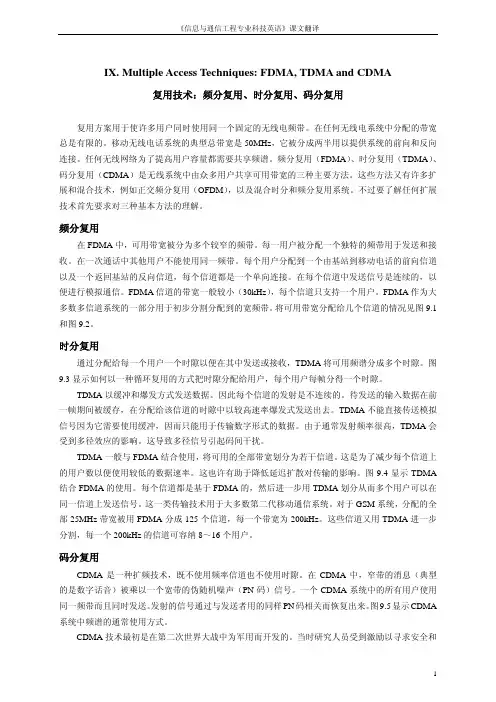
它的特点是在一个频域内分布着许多带有间隔的子载波△f=1/Tu其中,Tu是每个子载波的调制符号时间。
如图2-1所示,“OFDM子载波间隔”。
OFDM的传输是基于块的。
每个OFDM符号间隔之间,调制符号是并行发送的。
调制符号可以通过调制字母表得到,如QPSK,16QAM或64QAM,对于3GPP组织LTE,子载波间隔是相等的为15 kHz。
另一方面,子载波的数目取决于传输带宽,在一个10MHZ的频谱分配下,600个子载波可以有序传输。
当然,带宽减小了,子载波数目也相应减少,带宽增加了,子载波数目也相应增加。
图2-1 OFDM子载波间隔在OFDM传输时,物理资源经常被描述成一个时域—频域的网格坐标图。
在这个坐标图里一列对应一个OFDM子载波,一行对应一个OFDM子载波。
如图2-2所示,“OFDM时频网格”。
尽管子载波的频谱有重叠,但在理想情况下,是对OFDM子载波解调后不引起任何干扰的,这是因为对每一个子载波间隔的特殊选择,让它等于相应的解调符号率。
图2-2 OFDM时频网格以一定的频率f s= N ×△f进行采样的OFDM信号,是该size-N 的逆离散傅立叶变换(IDFT)的调制符号块a0, a1,...a N-1。
因此,OFDM调制可以通过IDFT处理再到数字-模拟的转换来实现。
(见图2-3,“OFDM调制”)。
在实际中,OFDM调制是以快速傅立叶反变换(IFFT)方式实现简单和快速的处理,通过选择IDFT size N 等于2m(m为整数)。
中英文对照外文翻译文献(文档含英文原文和中文翻译)原文:RESEARCH OF CELLULAR WIRELESS COMMUNATIONSYSTEMA wide variety of wireless communication systems have been developed to provide access to the communications infrastructure for mobile or fixed users in a myriad of operating environments. Most of today’s wireless systems are based on the cellular radio concept. Cellular communication systems allow a large number of mobile users to seamlessly and simultaneously communicate to wireless modems at fixed base stations using a limited amount of radio frequency (RF) spectrum. The RF transmissions received at the base stations from each mobile are translated to baseband, or to a wideband microwave link, and relayed to mobile switching centers (MSC), which connect the mobile transmissions with the Public Switched Telephone Network (PSTN). Similarly, communications from the PSTN are sent to the base station, where they are transmitted to the mobile. Cellular systems employ eitherfrequency division multiple access (FDMA), time division multiple access (TDMA), code division multiple access (CDMA), or spatial division multiple access (SDMA) .Wireless communication links experience hostile physical channel characteristics, such as time-varying multipath and shadowing due to large objects in the propagation path. In addition, the performance of wireless cellular systems tends to be limited by interference from other users, and for that reason, it is important to have accurate techniques for modeling interference. These complex channel conditions are difficult to describe with a simple analytical model, although several models do provide analytical tractability with reasonable agreement to measured channel data . However, even when the channel is modeled in an analytically elegant manner, in the vast majority of situations it is still difficult or impossible to construct analytical solutions for link performance when error control coding, equalization, diversity, and network models are factored into the link model. Simulation approaches, therefore, are usually required when analyzing the performance of cellular communication links.Like wireless links, the system performance of a cellular radio system is most effectively modeled using simulation, due to the difficulty in modeling a large number of random events over time and space. These random events, such as the location of users, the number of simultaneous users in the system, the propagation conditions, interference and power level settings of each user, and the traffic demands of each user, combine together to impact the overall performance seen by a typical user in the cellular system. The aforementioned variables are just a small sampling of the many key physical mechanisms that dictate the instantaneous performance of a particular user at any time within the system. The term cellular radio system, therefore, refers to the entire population of mobile users and base stations throughout the geographic service area, as opposed to a single link that connects a single mobile user to a single base station. To design for a particular system-level performance, such as the likelihood of a particular user having acceptable service throughout the system, it is necessary to consider the complexity of multiple users that are simultaneously using the system throughout the coverage area. Thus, simulation is needed to consider the multi-user effects upon any of the individual links between the mobile and the base station.The link performance is a small-scale phenomenon, which deals with the instantaneouschanges in the channel over a small local area, or small time duration, over which the average received power is assumed constant. Such assumptions are sensible in the design of error control codes, equalizers, and other components that serve to mitigate the transient effects created by the channel. However, in order to determine the overall system performance of a large number of users spread over a wide geographic area, it is necessary to incorporate large-scale effects such as the statistical behavior of interference and signal levels experienced by individual users over large distances, while ignoring the transient channel characteristics. One may think of link-level simulation as being a vernier adjustment on the performance of a communication system, and the system-level simulation as being a coarse, yet important, approximation of the overall level of quality that any user could expect at any time.Cellular systems achieve high capacity (e.g., serve a large number of users) by allowing the mobile stations to share, or reuse a communication channel in different regions of the geographic service area. Channel reuse leads to co-channel interference among users sharing the same channel, which is recognized as one of the major limiting factors of performance and capacity of a cellular system. An appropriate understanding of the effects of co-channel interference on the capacity and performance is therefore required when deploying cellular systems, or when analyzing and designing system methodologies that mitigate the undesired effects of co-channel interference. These effects are strongly dependent on system aspects of the communication system, such as the number of users sharing the channel and their locations. Other aspects, more related to the propagation channel, such as path loss, shadow fading (or shadowing), and antenna radiation patterns are also important in the context of system performance, since these effects also vary with the locations of particular users. In this chapter, we will discuss the application of system-level simulation in the analysis of the performance of a cellular communication system under the effects of co-channel interference. We will analyze a simple multiple-user cellular system, including the antenna and propagation effects of a typical system. Despite the simplicity of the example system considered in this chapter, the analysis presented can easily be extended to include other features of a cellular system.2 Cellular Radio SystemSystem-Level Description:Cellular systems provide wireless coverage over a geographic service area by dividing the geographic area into segments called cells as shown in Figure 2-1. The available frequency spectrum is also divided into a number of channels with a group of channels assigned to each cell. Base stations located in each cell are equipped with wireless modems that can communicate with mobile users. Radio frequency channels used in the transmission direction from the base station to the mobile are referred to as forward channels, while channels used in the direction from the mobile to the base station are referred to as reverse channels. The forward and reverse channels together identify a duplex cellular channel. When frequency division duplex (FDD) is used, the forward and reverse channels are split in frequency. Alternatively, when time division duplex (TDD) is used, the forward and reverse channels are on the same frequency, but use different time slots for transmission.Figure 2-1 Basic architecture of a cellular communications system High-capacity cellular systems employ frequency reuse among cells. This requires that co-channel cells (cells sharing the same frequency) are sufficiently far apart from each other to mitigate co-channel interference. Channel reuse is implemented by covering the geographic service area with clusters of N cells, as shown in Figure 2-2, where N is known as the cluster size.Figure 2-2 Cell clustering:Depiction of a three-cell reuse pattern The RF spectrum available for the geographic service area is assigned to each cluster, such that cells within a cluster do not share any channel . If M channels make up the entire spectrum available for the service area, and if the distribution of users is uniform over the service area, then each cell is assigned M/N channels. As the clusters are replicated over the service area, the reuse of channels leads to tiers of co-channel cells, and co-channel interference will result from the propagation of RF energy between co-channel base stations and mobile users. Co-channel interference in a cellular system occurs when, for example, a mobile simultaneously receives signals from the base station in its own cell, as well as from co-channel base stations in nearby cells from adjacent tiers. In this instance, one co-channel forward link (base station to mobile transmission) is the desired signal, and the other co-channel signals received by the mobile form the total co-channel interference at the receiver. The power level of the co-channel interference is closely related to the separation distances among co-channel cells. If we model the cells with a hexagonal shape, as in Figure 2-2, the minimum distance between the center of two co-channel cells, called the reuse distance ND, is(2-1)R3D N Nwhere R is the maximum radius of the cell (the hexagon is inscribed within the radius).Therefore, we can immediately see from Figure 2-2 that a small cluster size (small reuse distance ND), leads to high interference among co-channel cells.The level of co-channel interference received within a given cell is also dependent on the number of active co-channel cells at any instant of time. As mentioned before, co-channel cells are grouped into tiers with respect to a particular cell of interest. The number of co-channel cells in a given tier depends on the tier order and the geometry adopted to represent the shape of a cell (e.g., the coverage area of an individual base station). For the classic hexagonal shape, the closest co-channel cells are located in the first tier and there are six co-channel cells. The second tier consists of 12 co-channel cells, the third, 18, and so on. The total co-channel interference is, therefore, the sum of the co-channel interference signals transmitted from all co-channel cells of all tiers. However, co-channel cells belonging to the first tier have a stronger influence on the total interference, since they are closer to the cell where the interference is measured.Co-channel interference is recognized as one of the major factors that limits the capacity and link quality of a wireless communications system and plays an important role in the tradeoff between system capacity (large-scale system issue) and link quality (small-scale issue). For example, one approach for achieving high capacity (large number of users), without increasing the bandwidth of the RF spectrum allocated to the system, is to reduce the channel reuse distance by reducing the cluster size N of a cellular system . However, reduction in the cluster sizeincreases co-channel interference, which degrades the link quality.The level of interference within a cellular system at any time is random and must be simulated by modeling both the RF propagation environment between cells and the position location of the mobile users. In addition, the traffic statistics of each user and the type of channel allocation scheme at the base stations determine the instantaneous interference level and the capacity of the system.The effects of co-channel interference can be estimated by the signal-tointerference ratio (SIR) of the communication link, defined as the ratio of the power of the desired signal S, to the power of the total interference signal, I. Since both power levels S and I are random variables due to RF propagation effects, user mobility and traffic variation, the SIR is also a random variable. Consequently, the severity of the effects of co-channel interference onsystem performance is frequently analyzed in terms of the system outage probability, defined in this particular case as the probability that SIR is below a given threshold 0S IR . This isdx p ]SIR Pr[SIR P )x 0SIR 0SIR 0outpage (⎰=<= (2-2)Where is the probability density function (pdf) of the SIR. Note the distinction between the definition of a link outage probability, that classifies an outage based on a particular bit error rate (BER) or Eb/N0 threshold for acceptable voice performance, and the system outage probability that considers a particular SIR threshold for acceptable mobile performance of a typical user.Analytical approaches for estimating the outage probability in a cellular system, as discussed in before, require tractable models for the RF propagation effects, user mobility, and traffic variation, in order to obtain an expression for PSIR (x ). Unfortunately, it is very difficult to use analytical models for these effects, due to their complex relationship to the received signal level. Therefore, the estimation of the outage probability in a cellular system usually relies on simulation, which offers flexibility in the analysis. In this chapter, we present a simple example of a simulation of a cellular communication system, with the emphasis on the system aspects of the communication system, including multi-user performance, traffic engineering, and channel reuse. In order to conduct a system-level simulation, a number of aspects of the individual communication links must be considered. These include the channel model, the antenna radiation pattern, and the relationship between Eb/N0 (e.g., the SIR) and the acceptable performance.SIR(x)p翻译:蜂窝无线通信系统的研究摘要蜂窝通信系统允许大量移动用户无缝地、同时地利用有限的射频(radio frequency,RF)频谱与固定基站中的无线调制解调器通信。
mimo-ofdm无线通信技术及matlab实现英文版Title: MIMO-OFDM Wireless Communication Technology and MATLAB ImplementationIntroduction:MIMO-OFDM (Multiple-Input Multiple-Output Orthogonal Frequency Division Multiplexing) is a wireless communication technology that combines multiple antennas and orthogonal frequency division multiplexing to achieve high data rates, increased spectral efficiency, and improved system performance. In this article, we will provide a detailed and accurate overview of MIMO-OFDM technology, along with its MATLAB implementation.1. MIMO-OFDM Technology:1.1 Multiple-Input Multiple-Output (MIMO):- Definition: MIMO refers to the use of multiple antennas at both the transmitter and receiver to improve communication performance.- Benefits of MIMO: MIMO technology enables spatial multiplexing, diversity, and beamforming, leading to increased capacity, improved reliability, and enhanced coverage.1.2 Orthogonal Frequency Division Multiplexing (OFDM): - Definition: OFDM is a modulation technique that divides the available frequency spectrum into multiple orthogonal subcarriers.- Benefits of OFDM: OFDM enables high spectral efficiency, resistance to multipath fading, and robustness against frequency-selective fading channels.1.3 MIMO-OFDM Combination:- MIMO-OFDM combines the benefits of MIMO and OFDMto achieve high data rates, improved link reliability, and increased system capacity.- MIMO-OFDM utilizes spatial multiplexing totransmit multiple data streams simultaneously acrossdifferent subcarriers.2. MATLAB Implementation of MIMO-OFDM:2.1 Channel Modeling:- MATLAB provides various channel models that can be used to simulate realistic wireless communication scenarios, such as Rayleigh and Rician fading channels.- These channel models can be used to evaluate the performance of MIMO-OFDM systems under different channel conditions.2.2 Transmitter Design:- MATLAB provides tools for designing the MIMO-OFDM transmitter, including the generation of OFDM symbols, mapping of data streams to subcarriers, and spatial multiplexing using multiple antennas.- The transmitter design also includes the implementation of coding and modulation schemes to enhance the reliability and efficiency of the communication system.2.3 Receiver Design:- The receiver design in MATLAB involves the synchronization and demodulation of the received MIMO-OFDMsignals.- MATLAB provides algorithms for channel estimation, equalization, and decoding to mitigate the effects of channel impairments and enhance the overall system performance.2.4 Performance Evaluation:- MATLAB allows for the evaluation of various performance metrics of the MIMO-OFDM system, such as bit error rate (BER), signal-to-noise ratio (SNR), and throughput.- These performance metrics help in assessing the system's performance under different scenarios and optimizing the system parameters.Conclusion:MIMO-OFDM wireless communication technology combines the advantages of MIMO and OFDM to achieve high data rates, improved link reliability, and increased system capacity. MATLAB provides a comprehensive platform for the design, simulation, and evaluation of MIMO-OFDM systems, enabling researchers and engineers to analyze and optimize the performance of wireless communication systems.。
毕业设计(论文)外文文献翻译文献、资料中文题目:无线通信基础文献、资料英文题目:文献、资料来源:文献、资料发表(出版)日期:院(部):专业:通信工程班级:姓名:学号:指导教师:翻译日期: 2017.02.14毕业设计(论文)外文资料翻译外文出处无线通信基础(Fundamentals ofwireless communications by DavidTse)附件:1.外文资料翻译译文;2.外文原文附件1:外文资料翻译译文7.mimo:空间多路复用与信道建模本书我们已经看到多天线在无线通信中的几种不同应用。
在第3章中,多天线用于提供分集增益,增益无线链路的可靠性,并同时研究了接受分解和发射分解,而且,接受天线还能提供功率增益。
在第5章中,我们看到了如果发射机已知信道,那么多采用多幅发射天线通过发射波束成形还可以提供功率增益。
在第6章中,多副发射天线用于生产信道波动,满足机会通信技术的需要,改方案可以解释为机会波束成形,同时也能够提供功率增益。
章以及接下来的几章将研究一种利用多天线的新方法。
我们将会看到在合适的信道衰落条件下,同时采用多幅发射天线和多幅接收天线可以提供用于通信的额外的空间维数并产生自由度增益,利用这些额外的自由度可以将若干数据流在空间上多路复用至MIMO信道中,从而带来容量的增加:采用n副发射天线和接受天线的这类MIMO信道的容量正比于n。
过去一度认为在基站采用多幅天线的多址接入系统允许若干个用户同时与基站通信,多幅天线可以实现不同用户信号的空间隔离。
20世纪90年代中期,研究人员发现采用多幅发射天线和接收天线的点对点信道也会出现类似的效应,即使当发射天线相距不远时也是如此。
只要散射环境足够丰富,使得接受天线能够将来自不同发射天线的信号分离开,该结论就成立。
我们已经了解到了机会通信技术如何利用信道衰落,本章还会看到信道衰落对通信有益的另一例子。
将机会通信与MIMO技术提供的性能增益的本质进行比较和对比是非常的有远见的。
外文资料(一)On Orthogonal Space-Time Block Codes forMIMO-OFDM SystemsSpace-time code in mobile communication system, and orthogonal desing in multiple- antennas scneme are dicsussed. By the methods, data is encoded using a space- time block code and is split into several streams which are simultaneously transmitted by antennas. So a maximum- likelihood decoding algorithm can be used at the receiver to achieve the maximum diversity orderIntroductionMost work on wireless communications had focused on having an antenna array at only one end of the wireless link —usually at the receiver. Seminal papers by Gerard J. Foschini and Michael J. Gans[1], Foschini[2] and Emre Telatar[3] enlarged the scope of wireless communication possibilities by showing that for the highly-scattering environment substantial capacity gains are enabled when antenna arrays are used at both ends of a link. An alternative approach to utilizing multiple antennas relies on having multiple transmit antennas and only optionally multiple receive antennas. Proposed by Vahid Tarokh, Nambi Seshadri and Robert Calderbank, these space–time codes (STCs) achieve significant error rate improvements over single-antenna systems. Their original scheme was based on trellis codes but the simpler block codes were utilized by Siavash Alamouti,and later Vahid Tarokh, Hamid Jafarkhani and Robert Calderbank to develop space–time block-codes (STBCs)[4]. STC involves the transmission of multiple redundant copies of data to compensate for fading and thermal noise in the hope that some of them may arrive at the receiver in a better state than others. In the case of STBC in particular, the data stream to be transmitted is encoded in blocks, which are distributed among spaced antennas and across time. While it is necessary to have multiple transmit antennas, it is not necessary to have multiple receive antennas, although to do so improves performance. This process of receiving diverse copies of the data is known as diversity reception and is what was largely studied until Foschini's 1998 paper.An STBC is usually represented by a matrix. Each row represents a time slot and each column represents one antenna's transmissions over time.Here, s ij is the modulated symbol to be transmitted in time slot i from antenna j . There are to be T time slots and n T transmit antennas as well as n R receive antennas. This block is usually considered to be of 'length' TThe code rate of an STBC measures how many symbols per time slot it transmits on average over the course of one block. If a block encodes k symbols, the code-rate isTk rOnly one standard STBC can achieve full-rate (rate 1) — Alamouti's code OrthogonalitySTBCs as originally introduced, and as usually studied, are orthogonal. This means that the STBC is designed such that the vectors representing any pair of columns taken from the coding matrix is orthogonal. The result of this is simple, linear, optimal decoding at the receiver. Its most serious disadvantage is that all but one of the codes that satisfy this criterion must sacrifice some proportion of their data rate (see Alamouti's code).Moreover, there exist quasi-orthogonal STBCs that achieve higher data rates at the cost of inter-symbol interference (ISI). Thus, their error-rate performance is lower bounded by the one of orthogonal rate 1 STBCs, that provide ISI free transmissions due to orthogonality. Higher order STBCsTarokhet al. discovered a set of STBCs that are particularly straightforward, and coined the scheme's name. They also proved that no code for more than 2 transmit antennas could achieve full-rate. Their codes have since been improved upon (both by the original authors and by many others). Nevertheless, they serve as clear examples of why the rate cannot reach 1, and what other problems must be solved to produce 'good' STBCs. They also demonstrated the simple, linear decoding scheme that goes with their codes under perfect channel state information assumption.4 transmit antennasTwo straightforward codes for 4 transmit antennas are:⎥⎥⎥⎥⎥⎥⎥⎥⎥⎥⎥⎦⎤⎢⎢⎢⎢⎢⎢⎢⎢⎢⎢⎢⎣⎡------------=*1*2*3*4*2*1*4*3*3*4*1*2*4*3*2*112342143341243212/14c c c c c c c c c c c c c c c c c c c c c c c c c c c c c c c c C ,and()()()()⎥⎥⎥⎥⎥⎥⎥⎥⎥⎦⎤⎢⎢⎢⎢⎢⎢⎢⎢⎢⎣⎡-++--++--+---+----=222222222222*22*11*11*22*3*3*11*22*22*11*3*333*1*233214/3,4c c c c c c c c c c c c c c c c c c c c c c c c c c c c C These codes achieve rate-1/2 and rate-3/4 respectively, as for their 3-antenna counterparts.C 4,3 / 4 exhibits the same uneven power problems as C 3,3 / 4. An improved version of C 4,3 / 4 is⎥⎥⎥⎥⎦⎤⎢⎢⎢⎢⎣⎡----=1*2*32*1*33*1*23214/3,40000c c c c c c c c c c c c C which has equal power from all antennas in all time-slots. DecodingOne particularly attractive feature of orthogonal STBCs is that maximum likelihood decoding can be achieved at the receiver with only linear processing. In order to consider a decoding method, a model of the wireless communications system is needed.At time t , the signal i t r received at antenna j is:j t i t n i ij jt n s r T+=∑=1α,where αij is the path gain from transmit antenna i to receive antenna j , i t s is the signal transmitted by transmit antenna i and j t n is a sample of additive white Gaussian noise (AWGN).The maximum-likelihood detection rule is to form the decision variables)()(11i r R t j i n t n j j t i t T Rδαε∑∑===where δk (i ) is the sign of s i in the k th row of the coding matrix, εk (p ) = q denotes that s p is (up to a sign difference), the (k ,q ) element of the coding matrix, for i = 1,2...n T and then decide on constellation symbol s i that satisfies()()()h C C h h C r hC C h h C r rh C r cW H W H w H w HW H w H w +-=--=-=Re 2min arg min arg min arg ˆ22,with A the constellation alphabet. Despite its appearance, this is a simple, linear decoding scheme that provides maximal diversity. References[1] Gerard J. Foschini and Michael. J. Gans (January 1998). “On limits of wireless communications in a fading environment when using multiple antennas”. Wireless Personal Communications 6 (3): 311–335.[2] Gerard J. Foschini (autumn 1996). “Layered space -time architecture for wireless communications in a fading environment when using multi-element antennas”. Bell Labs Technical Journal 1 (2): 41–59.[3] I. Emre Telatar (November 1999). “Capacity of multi -antenna European Transactions on Telecommunications , 10 (6): 585–595.[4] Vahid Tarokh, Nambi Seshadri, and A. R. Calderbank (March 1998). "Space –time codes for high data rate wireless communication: Performance analysis and code construction". IEEE Transactions on Information Theory 44 (2): 744–765.译文基于MIMO-OFDM系统的正交空时分组码本文介绍了移动通信中的空时码, 针对多天线系统提出了空时分组码的正交设计理论, 可以采用高效的调制技术(QAM,PSK) ,由多天线同时发射。
附件1:外文资料翻译译文7.mimo:空间多路复用与信道建模本书我们已经看到多天线在无线通信中的几种不同应用。
在第3章中,多天线用于提供分集增益,增益无线链路的可靠性,并同时研究了接受分解和发射分解,而且,接受天线还能提供功率增益。
在第5章中,我们看到了如果发射机已知信道,那么多采用多幅发射天线通过发射波束成形还可以提供功率增益。
在第6章中,多副发射天线用于生产信道波动,满足机会通信技术的需要,改方案可以解释为机会波束成形,同时也能够提供功率增益。
这章以及接下来的几章将研究一种利用多天线的新方法。
我们将会看到在合适的信道衰落条件下,同时采用多幅发射天线和多幅接收天线可以提供用于通信的额外的空间维数并产生自由度增益,利用这些额外的自由度可以将若干数据流在空间上多路复用至MIMO 信道中,从而带来容量的增加:采用n副发射天线和接受天线的这类MIMO信道的容量正比于n。
过去一度认为在基站采用多幅天线的多址接入系统允许若干个用户同时与基站通信,多幅天线可以实现不同用户信号的空间隔离。
20世纪90年代中期,研究人员发现采用多幅发射天线和接收天线的点对点信道也会出现类似的效应,即使当发射天线相距不远时也是如此。
只要散射环境足够丰富,使得接受天线能够将来自不同发射天线的信号分离开,该结论就成立。
我们已经了解到了机会通信技术如何利用信道衰落,本章还会看到信道衰落对通信有益的另一例子。
将机会通信与MIMO技术提供的性能增益的本质进行比较和对比是非常的有远见的。
机会通信技术主要提供功率增益,改功率增益在功率受限系统的低信噪比情况下相当明显,但在宽带受限系统的高信噪比情况下则很不明显。
正如我们将看到的,MIMO技术不仅能够提供功率增益,还可以提供自由度增益,因此,MIMO技术成为在高信噪比情况下大幅度增加容量的主要工具。
MIMO通信是一个内容非常丰富的主题,对它的研究将覆盖本书其余章节。
本章集中研究能够实现空间多路复用的物理环境的属性,并阐明如何在MIMO统计信道模型中简明扼要地俘获这些属性。
中英文翻译(文档含英文原文和中文翻译)附件1:外文资料翻译译文通用移动通信系统的回顾1.1 UMTS网络架构欧洲/日本的3G标准,被称为UMTS。
UMTS是一个在IMT-2000保护伞下的ITU-T 批准的许多标准之一。
随着美国的CDMA2000标准的发展,它是目前占主导地位的标准,特别是运营商将cdmaOne部署为他们的2G技术。
在写这本书时,日本是在3G 网络部署方面最先进的。
三名现任运营商已经实施了三个不同的技术:J - PHONE 使用UMTS,KDDI拥有CDMA2000网络,最大的运营商NTT DoCoMo正在使用品牌的FOMA(自由多媒体接入)系统。
FOMA是基于原来的UMTS协议,而且更加的协调和标准化。
UMTS标准被定义为一个通过通用分组无线系统(GPRS)和全球演进的增强数据技术(EDGE)从第二代GSM标准到UNTS的迁移,如图。
这是一个广泛应用的基本原理,因为自2003年4月起,全球有超过847万GSM用户,占全球的移动用户数字的68%。
重点是在保持尽可能多的GSM网络与新系统的操作。
我们现在在第三代(3G)的发展道路上,其中网络将支持所有类型的流量:语音,视频和数据,我们应该看到一个最终的爆炸在移动设备上的可用服务。
此驱动技术是IP协议。
现在,许多移动运营商在简称为2.5G的位置,伴随GPRS的部署,即将IP骨干网引入到移动核心网。
在下图中,图2显示了一个在GPRS网络中的关键部件的概述,以及它是如何适应现有的GSM基础设施。
SGSN和GGSN之间的接口被称为Gn接口和使用GPRS隧道协议(GTP的,稍后讨论)。
引进这种基础设施的首要原因是提供连接到外部分组网络如,Internet或企业Intranet。
这使IP协议作为SGSN和GGSN之间的运输工具应用到网络。
这使得数据服务,如移动设备上的电子邮件或浏览网页,用户被起诉基于数据流量,而不是时间连接基础上的数据量。
中英文对照外文翻译(文档含英文原文和中文翻译)光纤通信技术摘要:光纤通信不仅可以应用在通信的主干线路中,还可以应用在电力通信控制系统中,进行工业监测、控制,而且在军事领域的用途也越来越为广泛。
光纤通信技术作为信息技术的重要支撑平台,在未来信息社会中将起到十分重要的作用。
关键词:光纤通信技术优势接入技术近年来随着传输技术和交换技术的不断进步,核心网已经基本实现了光纤化、数字化和宽带化。
同时,随着业务的迅速增长和多媒体业务的日益丰富,使得用户住宅网的业务需求也不只局限于原来的语音业务,数据和多媒体业务的需求已经成为不可阻挡的趋势,现有的语音业务接入网越来越成为制约信息高速公路建设的瓶颈,成为发展宽带综合业务数字网的障碍。
1 光纤通信技术定义光纤通信是利用光作为信息载体、以光纤作为传输的通信力式。
在光纤通信系统中,作为载波的光波频率比电波的频率高得多,而作为传输介质的光纤又比同轴电缆或导波管的损耗低得多,所以说光纤通信的容量要比微波通信大几十倍。
光纤是用玻璃材料构造的,它是电气绝缘体,因而不需要担心接地回路,光纤之间的中绕非常小,光波在光纤中传输,不会因为光信号泄漏而担心传输的信息被人窃听,光纤的芯很细,由多芯组成光缆的直径也很小,所以用光缆作为传输信道,使传输系统所占空间小,解决了地下管道拥挤的问题。
2 光纤通信技术优势2.1 频带极宽,通信容量大光纤比铜线或电缆有大得多的传输带宽,光纤通信系统的于光源的调制特性、调制方式和光纤的色散特性。
散波长窗口,单模光纤具有几十GHz·km的宽带。
对于单波长光纤通信系统,由于终端设备的电子瓶颈效应而不能发挥光纤带宽大的优势。
通常采用各种复杂技术来增加传输的容量,特别是现在的密集波分复用技术极大地增加了光纤的传输容量。
采用密集波分复术可以扩大光纤的传输容量至几倍到几十倍。
目前,单波长光纤通信系统的传输速率一般在2.5Gbps到1OGbps,采用密集波分复术实现的多波长传输系统的传输速率已经达到单波长传输系统的数百倍。
基于OFDM-MFSK的在快速衰落信道的鲁棒性传输摘要:我们提出了一个基于OFDM的传输方案,它适合在快速衰落环境中鲁棒性传输,在这个环境中估计不可能或非常困难获得一个可靠的信道。
我们的方案是以非相干检测的MFSK (M进制频移监控)和OFDM(正交频分复用)的组合为基础的。
非相干检测的OFDM-MFSK 允许任意相位用于发送器中的所有副载波。
一种可能性是:利用选择副载波相位的自由度,这样,该PAPR(峰均功率比)变小。
第二种可能性是:使用副载波相位发送附加数据。
这可以通过差分调制由所述OFDM MFSK方案所占用的子载波来实现。
这两种可能性都不会影响相关非相干检测的OFDM MFSK调制的鲁棒性。
Ⅰ介绍高速列车无线通信是一个典型的情况,在这种情况下会产生快速衰落信道。
未来的火车预计时速可达到v= 600公里/小时。
在这样的环境中获取一个可靠的信道估计是很困难的,同时一些数据包会包含与安全相关的控制数据,因此需要一个鲁棒性的传输方案。
对于多径信道,0FDM(正交频分复用)是一个可以避免符号间干扰的方法。
在本文中,我们分析了一个系统。
其中,结合OFDM的非相干检测的M进制频移键控(MFSK),产生一种非常简单的接收机,它不需要均衡和信道估计。
非相干检测的OFDM-MFSK允许发射任意相位的副载波。
结合OFDM的MFSK的缺点是它的低频谱效率。
为了减轻低频谱效率的影响,我们使用一种混合传输方法。
通过结合OFDM-MFSK和DPSK(差分相移键控)利用副载波的所有相位来传输更多的数据。
第二种可能性是选择子载波的相位,这样的话,发送信号的PAPR(峰均功率比)就会减小。
这两种方法都不会影响非相干检测相关的OFDM-MFSK。
Ⅱ系统模型我们使用一个时域取样的离散时间基带表示OFDM传输。
S是通过变换大小为N×1的发送码元x到时域中,使用归一化的IFFT和添加Ng个样本的循环前缀获得的。
并行到串行转换后,离散时间发送信号s(iΔt)与信道单位脉冲响应h(iΔt)卷积,并受到AWGN (高斯白噪声)的影响:G(iΔt)= S(iΔt)×H(iΔt)+ N(iΔt):(1)在接收端,从接受到的信号G(iΔt)中除去循环前缀,串并转换后通过FFT变换到频域,这样接收到的OFDM信号y能被独立检测。
OFDM技术的基本原理(论文)OFDM技术的基本原理现代社会对通信的依赖和要求越来越高,于是设计和开发效率更高的通信系统就成了通信工程界不断追求的目标。
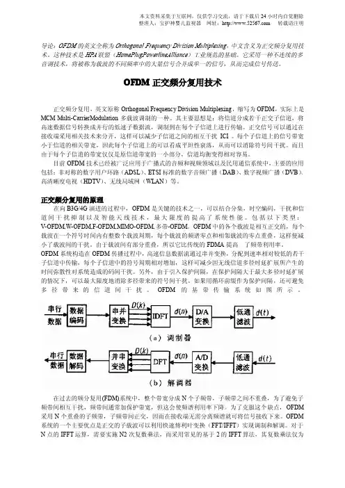
通信系统的效率,说到底就是频谱利用率和功率利用率。
特别是在无线通信的情况下,对这两个指标的要求往往更高,尤其是频谱利用率。
由于空间可用频谱资源是有限的,而无线应用却越来越多,使得无线频谱的使用受到各国政府的严格管理并统一规划。
于是,各种各样的具有较高频谱效率的通信技术不断被开发出来,OFDM(Orthogonal Frequency Division Multiplexing)是目前已知的频谱利用率最高的一种通信系统,它将数字调制、数字信号处理、多载波传输等技术有机结合在一起,使得它在系统的频谱利用率、功率利用率、系统复杂性方面综合起来有很强的竞争力,是支持未来移动通信特别是移动多媒体通信的主要技术之一。
OFDM是一种多载波传输技术,N个子载波把整个信道分割成N个子信道,N个子信道并行传输信息。
OFDM系统有许多非常引人注目的优点。
第一,OFDM具有非常高的频谱利用率。
普通的FDM系统为了分离开各子信道的信号,需要在相邻的信道间设置一定的保护间隔(频带),以便接收端能用带通滤波器分离出相应子信道的信号,造成了频谱资源的浪费。
OFDM系统各子信道间不但没有保护频带,而且相邻信道间信号的频谱的主瓣还相互重叠(见图1.5),但各子信道信号的频谱在频域上是相互正交的,各子载波在时域上是正交的,OFDM系统的各子信道信号的分离(解调)是靠这种正交性来完成的。
另外,OFDM 的个子信道上还可以采用多进制调制(如频谱效率很高的QAM),进一步提高了OFDM系统的频谱效率。
第二,实现比较简单。
当子信道上采用QAM或MPSK调制方式时,调制过程可以用IFFT完成,解调过程可以用FFT完成,既不用多组振荡源,又不用带通滤波器组分离信号。
第三,抗多径干扰能力强,抗衰落能力强。
中英文对照外文翻译文献(文档含英文原文和中文翻译)外文:OFDM BasicsINTRODUCTIONThe basic principle of OFDM is to split a high-rate data stream into a number of lowerrate streams that are transmitted simultaneously over a number of subcarriers. Because the symbol duration increases for the lower rate parallel subcarriers, the relative amount of dispersion in time caused by multipath delay spread is decreased. Inter symbol interference is eliminated almost completely by introducing a guard time in every OFDM symbol. In the guard time, the OFDM symbol is cyclically extended to avoidinter carrier interference In OFDM system design, a number of parameters are up for consideration, such as the number of subcarriers, guard time, symbol duration, subcarrier spacing,modulation type per subcarrier, and the type of forward error correction coding. The choice of parameters is influenced by system requirements such as available bandwidth,required bit rate, tolerable delay spread, and Doppler values. Some requirements are conflicting. For instance, to get a good delay spread tolerance, a large number of subcarriers with a small subcarrier spacing is desirable, but the opposite is true for a good tolerance against Doppler spread and phase noiseGENERATION OF SUBCARRIERS USING THE IFFT An OFDM signal consists of a sum of subcarriers that are modulated by using phase shift keying PSK or quadrature amplitude modulation QAM.If di are the complex QAM symbols, N is the number of subcarriers, T is the symbol duration, and f is the carrier frequency, then one OFDM symbol starting at t t, can be written as2.1In the literature, often the equivalent complex baseband notation is used, which is given by 2.2. In this representation, the real and imaginary parts correspond to the in-phase and quadrature parts of the OFDM signal, which have to be multiplied by a cosine and sine of the desired carrier frequency to produce the final OFDM signal.Figure 2.1 shows the operation of the OFDM modulator in a block diagram.2.2 Figure 2.1 OFDM modulatorAs an example,Figure2.2 shows four subcarriers from one OFDM signal. In this example, all subcarriers have the same phase and amplitude, but in practice the amplitudes and phases may be modulated differently for each subcarrier. Note that each subcarrier has exactly an integer number of cycles in the interval T, and the number of cycles between adjacent subcarriers differs by exactly one. This property accounts forthe orthogonality between the subcarriers. For instance, if the jth subcarrier from 2.2 is demodulated by down converting the signal with a frequency of j/T and then integrating the signal over T seconds, the result is as written in 2.3. By looking at the intermediate result, it can be seen that a complex carrier is integrated over T seconds.For the demodulated subcarrier j, this integration gives the desired output multiplied by a constant factor T, which is the QAM value for that particular subcarrier. For all other subcarriers, the integration is zero, because the frequency difference produces an integer number of cycles within the integration interval T,such that the integration result is always zero.2.3The orthogonality of the different OFDM subcarriers can also be demonstrated in another way. According to 2.1, each OFDM symbol contains subcarriers that are nonzero over a T-second interval. Hence, the spectrumof a single symbol is a convolution of a group of Dirac pulses located at the subcarrier frequencies with the spectrum of a square pulse that is one for a T-second period and zero otherwise. The amplitude spectrum of the square pulse is equal to sincnJT, which has zeros for all frequencies f that are an integer multiple of 1IT. This effect is shown in Figure 2.2,which shows the overlapping sinc spectra of individual subcarriers. At the imum of each subcarrier spectrum, all other subcarrier spectra are zero. Because an OFDM receiver essentially calculates the spectrum values at those points that correspond to the ima of individual subcarriers, it can demodulate each subcarrier free from any interference from the other subcarriers. Basically, Figure 2.3 shows that the OFDM spectrum fulfills Nyquist's criterium for an intersymbol interference free pulse shape.Notice that the pulse shape is present in the frequency domainand not in the time domain, for which the Nyquist criterium usually is applied. Therefore, instead of intersymbol interference ISI, it is intercarrier interference ICI that is avoided by havingthe imum of one subcarrier spectrum correspond to zero crossings of all the others.Figure 2.2 Example of four subcarriers within one OFDM symbolThe complex baseband OFDM signal as defined by 2.2 is in fact nothing more than the inverse Fourier transform of N, QAM input symbols.The time discrete equivalent is the inverse discrete Fourier transform IDFT, which is given by 2.4,where the time t is replaced by a sample number n. In practice, this transform can be implemented very efficiently by the inverse fast Fourier transform IFFT. An N point IDFT requires a total of N~ complex multiplications-which are actually only phase rotations. Of course, there are also additions necessary to do an IDFT, but since the hardware complexity of an adder is significantly lower than that of a multiplier or phase rotator, only the multiplications are used here for comparison. The IFFT drastically reduces the amount of calculations by exploiting the regularity of the operations in the IDFT. Using the radix-2 algorithm, an N-point IFFT requires only N/2.log2N complex multiplications [I]. For a 16-point transform, for instance, the difference is 256 multiplications for the IDFT versus 32 for the IFFT-a reduction by a factor of 8!This difference grows for larger numbers of subcarriers, as the IDFT complexity grows quadratically with N, while the IFFT complexity only grows slightly faster than linear.2.4The number of multiplications in the JFFT can be reduced even further by using a radix-4 algorithm. This technique makes use of the fact that in a four-point IFFT,there are only multiplications by 1,-1 j,-j, which actually do not need to be implemented by a full multiplier, butrather by a simple add or subtract and a switch of real and imaginary parts in the case of multiplications by j or -j. In the radix-4 algorithm, the transform is split into a number of these trivial four-point transforms,and non-trivial multiplications only have to be performed between stages of these four-point transforms. In this way, an N-point FFT using the radix4 algorithm requires only 3/8Nlog2N-2 complex multiplications or phase rotations and Mog2N complex additions [I]GUARD TIME AND CYCLIC EXTENSIONOne of the most important reasons to do OFDM is the efficient way it deals with multipath delay spread. By dividing the input datastream in Ns subcarriers, the symbol duration is made Ns times smaller, which also reduces the relative multipath delay spread, relative to the symbol time; by the same factor. To eliminate intersymbol interference almost completely, a guard time is introduced for each OFDM symbol. The guard time is chosen larger than the expected delay spread, such that multipath components from one symbol cannot interfere with the next symbol. The guard time could consist of no signal at all. In that case, however, the problem of intercarrier interference ICI would arise. ICI is crosstalk between different subcarriers, which means they are no longer orthogonal. This effect is illustrated in Figure 2.6. In this example, a subcarrier 1 and a delayed subcarrier 2 are shown. When an OFDM receivertries to demodulate the first subcarrier, it will encounter some interference fromthe second subcarrier, because within the FFT interval, there is no integer number of cycles difference between subcarrier 1 and 2. At the same time, there will be crosstalk from the first to the second subcarrier for the same reason.Figure 2.6 Effect of multipath with zero signal in the guard time; the delayed subcarrier 2 causes ICI on subcarrier 1 and vice versa.CHOICE OF OFDM PARAMETERSThe choice of various OFDM parameters is a trade off between various, often conflicting requirements. Usually, there are three main requirements to start with:bandwidth, bit rate, and delay spread. The delay spread directly dictates the guard time.As a rule, the guard time should be about two to four times the root-mean-squared delay spread. This value depends on the type of coding and QAM modulation. Higher order QAM like 64-QAM is more sensitive to ICI and IS1 than QPSK, while heavier coding obviously reduces the sensitivity to such interference.Now that the guard time has been set, the symbol duration can be fixed. To minimize the signal-to-noise ratio SNR loss caused by the guard time, it is desirable to have the symbol duration much larger than the guard time. It cannot be arbitrarily large, however, because a larger symbol duration means more subcarriers with a smaller subcarrier spacing, a larger implementation complexity, and more sensitivity to phase noiseand frequency offset [2], as well as an increased peak-to-average power ratio [3,4]. Hence, a practical design choice is to make the symbol duration at least five times the guard time, which implies a 1-dB SNR loss because of the guard time.译文:OFDM基础介绍OFDM的基本原理是将一串高速数据流变成同时传输在一些副载波的低速率数据流。