【原创】R语言版数据挖掘常用模型构建示例附代码数据
- 格式:doc
- 大小:71.00 KB
- 文档页数:5


务(附代码数据),咨询QQ:3025393450有问题到百度搜索“大数据部落”就可以了欢迎登陆官网:/datablogR语言挖掘公告板数据文本挖掘研究分析## Registered S3 methods overwritten by 'ggplot2':## method from## [.quosures rlang## c.quosures rlang## print.quosures rlang我们对1993年发送到20个Usenet公告板的20,000条消息进行从头到尾的分析。
此数据集中的Usenet公告板包括新闻组用于政治,宗教,汽车,体育和密码学等主题,并提供由许多用户编写的丰富文本。
该数据集可在/~jason/20Newsgroups/(该20news-bydate.tar.gz文件)上公开获取,并已成为文本分析和机器学习练习的热门。
1预处理我们首先阅读20news-bydate文件夹中的所有消息,这些消息组织在子文件夹中,每个消息都有一个文件。
我们可以看到在这样的文件用的组合read_lines(),map()和unnest()。
请注意,此步骤可能需要几分钟才能读取所有文档。
library(dplyr)library(tidyr)library(purrr)务(附代码数据),咨询QQ:3025393450有问题到百度搜索“大数据部落”就可以了欢迎登陆官网:/databloglibrary(readr)training_folder <- "data/20news-bydate/20news-bydate-train/"# Define a function to read all files from a folder into a data frameread_folder <-function(infolder) {tibble(file =dir(infolder, s =TRUE)) %>%mutate(text =map(file, read_lines)) %>%transmute(id =basename(file), text) %>%unnest(text)}# Use unnest() and map() to apply read_folder to each subfolderraw_text <-tibble(folder =dir(training_folder, s =TRUE)) %>%unnest(map(folder, read_folder)) %>%transmute(newsgroup =basename(folder), id, text)raw_text## # A tibble: 511,655 x 3## newsgroup id text## <chr> <chr> <chr>## 1 alt.atheism 49960 From: mathew <mathew@>## 2 alt.atheism 49960 Subject: Alt.Atheism FAQ: Atheist Resources## 3 alt.atheism 49960 Summary: Books, addresses, music -- anything related to atheism## 4 alt.atheism 49960 Keywords: FAQ, atheism, books, music, fiction, addresses, contacts## 5 alt.atheism 49960 Expires: Thu, 29 Apr 1993 11:57:19 GMT## 6 alt.atheism 49960 Distribution: world## 7 alt.atheism 49960 Organization: Mantis Consultants, Cambridge. UK.## 8 alt.atheism 49960 Supersedes: <19930301143317@>## 9 alt.atheism 49960 Lines: 290## 10 alt.atheism 49960 ""## # … with 511,645 more rows请注意该newsgroup列描述了每条消息来自哪20个新闻组,以及id列,用于标识该新闻组中的唯一消息。

【最新】R语⾔关联分析模型报告案例附代码数据【原创】附代码数据有问题到淘宝找“⼤数据部落”就可以了关联分析⽬录⼀、概括 (1)⼆、数据清洗 (1)2.1公⽴学费(NPT4_PUB) (1)2.2毕业率(Graduation.rate) (1)2.3贷款率(GRAD_DEBT_MDN_SUPP) (2)2.4偿还率(RPY_3YR_RT_SUPP) (2)2.5毕业薪⽔(MD_EARN_WNE_P10)。
(3)2.6 私⽴学费(NPT4_PRIV) (3)2.7 ⼊学率(ADM_RATE_ALL) (4)三、Apriori算法 (4)3.1 相关概念 (5)3.2 算法流程 (6)3.3 优缺点 (7)四、模型建⽴及结果 (8)4.1 公⽴模型 (8)4.2 私⽴模型 (11)⼀、概括对7703条样本数据,分别根据公⽴学费和私⽴学费差异,建⽴公⽴模型和私⽴模型,进⾏关联分析。
⼆、数据清洗2.1公⽴学费(NPT4_PUB)此字段,存在4个负值,与实际情况不符,故将此四个值重新定义为NULL。
重新定义后,NULL值的占⽐为75%,占⽐很⼤,不能直接将NULL值删除或者进⾏插补,故将NULL单独作为⼀个取值分组。
对⾮NULL的值按照等⽐原则进⾏分组,分组结果如下:A:[0,5896]B:(5896,7754]C:(7754, 9975]D:(9975, 13819]E:(13819, +]分组后取值分布为:2.2毕业率(Graduation.rate)将PrivacySuppressed值重新定义为NULL,重新定义后,NULL值的占⽐为20%,占⽐较⼤,不适合直接删除或进⾏插补,故将NULL单独作为⼀个取值分组。
对⾮NULL值根据等⽐原则进⾏分组,分组结果如下:A:[0,0.29]B:(0.29,0.47]C:(0.47, 0.61]D:(0.61, 0.75]E:(0.75, +]分组后取值分布为:2.3贷款率(GRAD_DEBT_MDN_SUPP)将PrivacySuppressed值重新定义为NULL,重新定义后,NULL值的占⽐为20%,占⽐较⼤,不适合直接删除或进⾏插补,故将NULL单独作为⼀个取值分组。
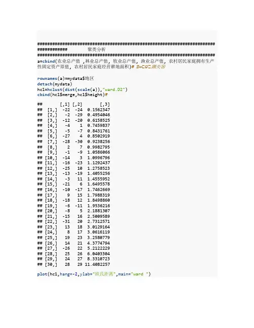
####################################################################### ############ 聚类分析####################################################################### a=cbind(农业总产值 ,林业总产值, 牧业总产值, 渔业总产值, 农村居民家庭拥有生产性固定资产原值, 农村居民家庭经营耕地面积)# ⭞↚⭞Ѡ⭞䠅㚐㊱rownames(a)=mydata$地区detach(mydata)hc1=hclust(dist(scale(a)),"ward.D2")cbind(hc1$merge,hc1$height)### [,1] [,2] [,3]## [1,] -22 -24 0.1562347## [2,] -2 -29 0.4954046## [3,] -12 -20 0.6158525## [4,] -4 1 0.7459837## [5,] -5 -7 0.8431761## [6,] -27 4 0.8502919## [7,] -28 -30 0.9238256## [8,] 2 7 0.9982795## [9,] -1 -9 1.0586066## [10,] -14 3 1.0996796## [11,] -16 -23 1.1292437## [12,] -25 10 1.2758523## [13,] -13 -19 1.4055256## [14,] -3 11 1.4555952## [15,] -21 6 1.6495578## [16,] -10 -17 1.7462669## [17,] 9 15 1.7988319## [18,] -18 12 1.8498860## [19,] -6 -11 1.9536216## [20,] -8 5 2.1881307## [21,] -15 16 2.5009589## [22,] -31 20 2.7312571## [23,] 13 18 3.0129164## [24,] 8 17 3.0616119## [25,] 19 23 3.2580779## [26,] 14 21 4.3774794## [27,] -26 22 5.2122229## [28,] 25 26 6.0403304## [29,] 24 27 8.3310723## [30,] 28 29 11.4082257plot(hc1,hang=-2,ylab="欧氏距离",main="ward ")cutree(hc1,3)## 北京天津河北山西内蒙辽宁吉林黑龙江上海江苏## 1 1 2 1 3 2 3 3 1 2## 浙江安徽福建江西山东河南湖北湖南广东广西## 2 2 2 2 2 2 2 2 2 2## 海南重庆四川贵州云南西藏陕西甘肃青海宁夏## 1 1 2 1 2 3 1 1 1 1## 新疆## 3library(NbClust)# 加载包res<-NbClust(a, distance ="euclidean", min.nc=2, max.nc=8,method ="complete", index ="ch")res$All.index## 2 3 4 5 6 7 8## 22.4859 64.2952 95.0505 91.2070 112.2167 126.6607 125.0580res$Best.nc## Number_clusters Value_Index## 7.0000 126.6607res$Best.partition## 北京天津河北山西内蒙辽宁吉林黑龙江上海江苏## 1 2 2 3 4 5 5 4 6 1## 浙江安徽福建江西山东河南湖北湖南广东广西## 5 1 1 3 2 1 3 3 3 1## 海南重庆四川贵州云南西藏陕西甘肃青海宁夏## 1 1 1 1 2 7 1 2 5 5## 新疆## 4####################################################################### ############ 因子分析####################################################################### x=ascale(x,center=T,scale=T)## 农业总产值林业总产值牧业总产值渔业总产值## 北京 -1.22777296 -0.68966546 -1.0576108 -0.717868590## 天津 -1.20072019 -1.32628581 -1.1287831 -0.587405030## 河北 1.44015787 -0.40768816 1.2735925 -0.276307864## 山西 -0.60736290 -0.39313054 -0.8459665 -0.730089499## 内蒙 -0.31173176 -0.16449038 0.3536925 -0.682760278## 辽宁 0.02317599 0.21376291 1.0886323 0.905582647## 吉林 -0.31664133 -0.16033106 0.3705164 -0.661159286## 黑龙江 0.73000004 0.28496065 0.6928325 -0.543827843## 上海 -1.22304555 -1.24358878 -1.1769433 -0.598687930## 江苏 1.32304764 -0.14014613 0.5106958 2.558246143## 浙江 -0.25945707 0.37842297 -0.4799669 1.088655075## 安徽 0.32193142 1.20245730 0.3549653 0.277626262## 福建 -0.22816878 1.77681021 -0.5790521 1.668371030## 江西 -0.46544975 1.43990544 -0.1820088 0.139953438## 山东 2.22835882 -0.05133246 2.0610374 2.643122498## 河南 2.22683767 0.36264203 2.0166955 -0.521101240## 湖北 0.88705181 -0.13647615 0.6684891 0.925656025## 湖南 1.03609706 1.81987138 0.8945726 -0.002409428## 广东 0.65132842 1.36442604 0.3760463 1.697020485## 广西 0.19109441 1.64358969 0.2862654 0.136415807## 海南 -0.95958625 0.32594217 -0.9698633 -0.119446069## 重庆 -0.61246376 -0.82851329 -0.6191076 -0.632081027## 四川 1.13921636 0.49292656 2.0375425 -0.313747797## 贵州 -0.59146827 -0.69749477 -0.6664339 -0.677051827## 云南 -0.10569354 1.40222691 0.0524867 -0.583545796## 西藏 -1.33060989 -1.32909946 -1.1967954 -0.752065694## 陕西 0.01099770 -0.64550329 -0.4072439 -0.713500151## 甘肃 -0.48272891 -1.11489458 -0.9441448 -0.747831257## 青海 -1.27264229 -1.30451055 -1.0825979 -0.751154486## 宁夏 -1.16021392 -1.24089745 -1.1284759 -0.716850181## 新疆 0.14646191 -0.83389594 -0.5730687 -0.711758136## 农村居民家庭拥有生产性固定资产原值农村居民家庭经营耕地面积## 北京 -0.521919855 -0.69519658 ## 天津 -0.036498322 -0.33578982 ## 河北 0.004069841 -0.23262677 ## 山西 -0.824825602 -0.02962851 ## 内蒙 1.179852466 2.59936535## 辽宁 0.730243656 0.39633505## 吉林 0.724094855 1.89053536## 黑龙江 1.396721068 3.65096289## 上海 -1.404513394 -0.77506475 ## 江苏 -0.340308064 -0.44560856 ## 浙江 0.499884752 -0.68188522 ## 安徽 -0.279565363 -0.23262677 ## 福建 -0.618739413 -0.61865625 ## 江西 -0.805278639 -0.33911766 ## 山东 0.133404538 -0.31582278 ## 河南 -0.500048919 -0.32247846 ## 湖北 -0.721961668 -0.29252790 ## 湖南 -0.917381131 -0.45559208 ## 广东 -0.957062704 -0.68521306 ## 广西 -0.615649655 -0.40567447 ## 海南 -0.663204069 -0.58537785 ## 重庆 -0.570175555 -0.43229719 ## 四川 -0.420353046 -0.48221480 ## 贵州 -0.604823220 -0.46890344 ## 云南 0.118332502 -0.32913414 ## 西藏 3.590383141 -0.23262677 ## 陕西 -0.572497480 -0.35575687 ## 甘肃 0.165991341 0.04358397## 青海 0.415065901 -0.25259382 ## 宁夏 0.655330865 0.36638449## 新疆 1.761431173 1.05524743 ## attr(,"scaled:center")## 农业总产值林业总产值## 1514.206129 111.20612 9## 牧业总产值渔业总产值## 877.092581 280.83903 2## 农村居民家庭拥有生产性固定资产原值农村居民家庭经营耕地面积## 17865.076774 2.58903 2## attr(,"scaled:scale")## 农业总产值林业总产值## 1097.854553 81.74416 7## 牧业总产值渔业总产值## 683.552567 373.13101 0## 农村居民家庭拥有生产性固定资产原值农村居民家庭经营耕地面积## 9767.757883 3.00495 2cor(x)### 农业总产值林业总产值牧业总产值## 农业总产值 1.00000000 0.4304367 0.9148545 ## 林业总产值 0.43043666 1.0000000 0.4593615 ## 牧业总产值 0.91485445 0.4593615 1.0000000 ## 渔业总产值 0.51598365 0.4351225 0.4103977 ## 农村居民家庭拥有生产性固定资产原值 -0.16652881 -0.3495913 -0.1017802## 农村居民家庭经营耕地面积 0.04040478 -0.0961515 0.1426829## 渔业总产值## 农业总产值 0.5159836## 林业总产值 0.4351225## 牧业总产值 0.4103977## 渔业总产值 1.0000000## 农村居民家庭拥有生产性固定资产原值 -0.2131248## 农村居民家庭经营耕地面积 -0.2669966## 农村居民家庭拥有生产性固定资产原值## 农业总产值 -0.1665288 ## 林业总产值 -0.3495913 ## 牧业总产值 -0.1017802 ## 渔业总产值 -0.2131248 ## 农村居民家庭拥有生产性固定资产原值 1.0000000 ## 农村居民家庭经营耕地面积 0.5316341 ## 农村居民家庭经营耕地面积## 农业总产值 0.04040478## 林业总产值 -0.09615150## 牧业总产值 0.14268286## 渔业总产值 -0.26699659## 农村居民家庭拥有生产性固定资产原值 0.53163410## 农村居民家庭经营耕地面积 1.00000000FA=factanal(x,3,scores="regression")FA#### Call:## factanal(x = x, factors = 3, scores = "regression")#### Uniquenesses:## 农业总产值林业总产值## 0.134 0.64 9## 牧业总产值渔业总产值## 0.005 0.00 5## 农村居民家庭拥有生产性固定资产原值农村居民家庭经营耕地面积## 0.005 0.61 0#### Loadings:## Factor1 Factor2 Factor3## 农业总产值 0.902 0.231## 林业总产值 0.460 -0.274 0.253## 牧业总产值 0.989 0.100## 渔业总产值 0.335 -0.172 0.924## 农村居民家庭拥有生产性固定资产原值 -0.185 0.980## 农村居民家庭经营耕地面积 0.120 0.569 -0.227#### Factor1 Factor2 Factor3## SS loadings 2.164 1.396 1.032## Proportion Var 0.361 0.233 0.172## Cumulative Var 0.361 0.593 0.765#### The degrees of freedom for the model is 0 and the fit was 0.0338A=FA$loadings#D=diag(FA$uniquenesses)#cancha=cor(x)-A%*%t(A)-Dsum(cancha^2)## [1] 0.01188033FA$scores## Factor1 Factor2 Factor3## 北京 -0.9595745 -0.700059511 -0.55760316## 天津 -1.0947804 -0.236528598 -0.28377148## 河北 1.3398849 0.269241913 -0.72734450## 山西 -0.6949304 -0.952525400 -0.71168863## 内蒙 0.3022926 1.274620864 -0.61477840## 辽宁 0.9086974 0.898645857 0.80686141## 吉林 0.3617131 0.823049845 -0.69568729## 黑龙江 0.6377695 1.558056539 -0.53064438## 上海 -1.0020542 -1.600313046 -0.58279912## 江苏 0.2978404 -0.338175607 2.58332275## 浙江 -0.6586307 0.351125849 1.47562686## 安徽 0.3633716 -0.220261996 0.12915299## 福建 -0.7017677 -0.799773443 1.90201088## 江西 -0.1252221 -0.843258690 0.03964935## 山东 1.8098550 0.433178408 2.27098864## 河南 2.1841524 -0.072629248 -1.35570609## 湖北 0.6625677 -0.618906179 0.64211420## 湖南 1.0200226 -0.733225411 -0.50075826## 广东 0.3057090 -0.945233885 1.54225085## 广西 0.3420343 -0.562216144 -0.07785160## 海南 -0.9131785 -0.847172077 0.04381513## 重庆 -0.5087268 -0.661768675 -0.62025496## 四川 2.1397385 -0.003827953 -1.11031362## 贵州 -0.5463126 -0.703696201 -0.66210885## 云南 0.1044516 0.146947680 -0.63418799## 西藏 -1.5214222 3.342858193 0.36144124## 陕西 -0.2687306 -0.616728372 -0.78286620## 甘肃 -0.8904189 0.010720625 -0.48059064## 青海 -1.0791206 0.225711752 -0.37974261## 宁夏 -1.1481591 0.456190239 -0.27546552## 新疆 -0.6670714 1.665952673 -0.21307102FA=factanal(x,3,scores="regression")#FA#### Call:## factanal(x = x, factors = 3, scores = "regression")#### Uniquenesses:## 农业总产值林业总产值## 0.134 0.64 9## 牧业总产值渔业总产值## 0.005 0.00 5## 农村居民家庭拥有生产性固定资产原值农村居民家庭经营耕地面积## 0.005 0.61 0#### Loadings:## Factor1 Factor2 Factor3## 农业总产值 0.902 0.231## 林业总产值 0.460 -0.274 0.253## 牧业总产值 0.989 0.100## 渔业总产值 0.335 -0.172 0.924## 农村居民家庭拥有生产性固定资产原值 -0.185 0.980## 农村居民家庭经营耕地面积 0.120 0.569 -0.227#### Factor1 Factor2 Factor3## SS loadings 2.164 1.396 1.032## Proportion Var 0.361 0.233 0.172## Cumulative Var 0.361 0.593 0.765#### The degrees of freedom for the model is 0 and the fit was 0.0338 biplot(FA$scores,FA$loadings)######################################################################## ########## 主成分分析####################################################################### # mydata<-read.csv("cosume.csv",header=TRUE)x=aPCA=princomp(x)# 分分析summary(PCA)## Importance of components:## Comp.1 Comp.2 Comp.3 Comp.4## Standard deviation 9611.2440729 1.248877e+03 3.201426e+02 2.211289e+02## Proportion of Variance 0.9817713 1.657641e-02 1.089277e-03 5.1968 75e-04## Cumulative Proportion 0.9817713 9.983477e-01 9.994370e-01 9.9995 67e-01## Comp.5 Comp.6## Standard deviation 6.377898e+01 2.299907e+00## Proportion of Variance 4.323210e-05 5.621753e-08## Cumulative Proportion 9.999999e-01 1.000000e+00plot(PCA)screeplot(PCA,type="lines")# ⻄⭞ഴPCA$loadings##### Loadings:## Comp.1 Comp.2 Comp.3 Comp.4 Comp. 5## 农业总产值 0.847 0.529 ## 林业总产值 -0.994 ## 牧业总产值 0.510 0.340 -0.786 ## 渔业总产值 0.147 -0.939 -0.304 ## 农村居民家庭拥有生产性固定资产原值 1.000 ## 农村居民家庭经营耕地面积## Comp.6## 农业总产值## 林业总产值## 牧业总产值## 渔业总产值## 农村居民家庭拥有生产性固定资产原值## 农村居民家庭经营耕地面积 1.000#### Comp.1 Comp.2 Comp.3 Comp.4 Comp.5 Comp.6## SS loadings 1.000 1.000 1.000 1.000 1.000 1.000## Proportion Var 0.167 0.167 0.167 0.167 0.167 0.167## Cumulative Var 0.167 0.333 0.500 0.667 0.833 1.000diag(1/sqrt(diag(cor(x))))%*%eigen(cor(x))$vectors%*%diag(sqrt(eigen(co r(x))$values))# ⭞⭞䠅фѱᡆ分的⭞ީ⭞䱫## [,1] [,2] [,3] [,4] [,5]## [1,] 0.8748914 0.33002393 -0.05962134 -0.2919961 0.03333473## [2,] 0.7199843 -0.09695761 0.39747812 0.5280225 0.18691501## [3,] 0.8358325 0.42778470 0.06215717 -0.2657004 0.10009450## [4,] 0.7239860 -0.13749802 -0.54651176 0.3113087 -0.24595467## [5,] -0.4283184 0.72257821 -0.37626680 0.2240839 0.32017966## [6,] -0.1942551 0.86197649 0.26492953 0.1648656 -0.34904716## [,6]## [1,] 0.189001599## [2,] 0.022088666## [3,] -0.184133750## [4,] -0.029268951## [5,] 0.010900009## [6,] 0.007698218print(-loadings(PCA),cutoff=0.001)#### Loadings:## Comp.1 Comp.2 Comp.3 Comp.4 Comp. 5## 农业总产值 0.019 -0.847 0.041 -0.529 0.027 ## 林业总产值 0.003 -0.026 0.036 0.096 0.994 ## 牧业总产值 0.007 -0.510 -0.340 0.786 -0.077 ## 渔业总产值 0.008 -0.147 0.939 0.304 -0.068 ## 农村居民家庭拥有生产性固定资产原值 -1.000 -0.021 0.006 -0.002 0.002 ## 农村居民家庭经营耕地面积 -0.003 0.003 ## Comp.6## 农业总产值## 林业总产值 0.003## 牧业总产值 0.001## 渔业总产值 -0.002## 农村居民家庭拥有生产性固定资产原值## 农村居民家庭经营耕地面积 -1.000#### Comp.1 Comp.2 Comp.3 Comp.4 Comp.5 Comp.6## SS loadings 1.000 1.000 1.000 1.000 1.000 1.000## Proportion Var 0.167 0.167 0.167 0.167 0.167 0.167## Cumulative Var 0.167 0.333 0.500 0.667 0.833 1.000####################################################################### ##### 条形图####################################################################### country<-mydata$地区percent<-mydata$农业总产值d<-data.frame(country,percent)# png("d:\\test2.png",width=2048,height=2048)f<-function(name,value) {xsize=200plot(0, 0,xlab="",ylab="",axes=FALSE,xlim=c(-xsize,xsize),ylim=c(-xsize,xsize))for(i in 1:length(name)){info =name[i]percent =value[i]k =(1:(360*percent/100)*10)/10r=xsize*(length(name)-i+1)/length(name)#print(r)x=r*sin(k/180*pi)y=r*cos(k/180*pi)text(-18,r,info,pos=2,cex=0.7)text(-9,r,paste(percent,"%"),cex=0.7)lines(x,y,col="red")}}f(country,percent)####################################################################### ###### 柱状图####################################################################### library(RColorBrewer)pv<-percentid<-countrycol<-c(brewer.pal(9, "YlOrRd")[1:9],brewer.pal(9, "Blues")[1:9]) barplot(pv,col=col,horiz =TRUE,xlim=c(-8000.00,5000))title(main=list("农业总产值",cex=2),sub="",ylab="地区")text(y=seq(from=0.7,length.out=31,by=1.2),x=-450.00,labels=id)legend("topleft",legend=rev(id),pch=10,col=rev(col),ncol=2)。

数据挖掘决策树r语言数据挖掘决策树是一种常用的机器学习算法,它能够从数据集中提取出有用的规律,帮助我们做出更好的决策。
在这篇文章中,我们将介绍如何使用R语言来构建决策树,并通过一个实例来演示其应用。
我们需要准备好数据集。
在这个例子中,我们将使用一个虚构的数据集,其中包含了一些人的个人信息和他们是否购买了某个产品的记录。
我们可以使用下面的代码来导入数据集:```rdata <- read.csv("data.csv",header=TRUE)```接下来,我们需要对数据集进行一些预处理。
首先,我们需要将一些非数值型的属性转换成数值型,这样才能在决策树中使用。
例如,性别属性通常可以转换成0/1表示男女。
我们还需要处理一些缺失值,通常使用均值或中位数进行填充。
我们可以使用下面的代码来进行预处理:```rdata$Sex <- ifelse(data$Sex == "Male", 0, 1) # 将性别转换为0/1data$Age[is.na(data$Age)] <- median(data$Age, na.rm=TRUE)# 使用中位数填充缺失值```接下来,我们可以开始构建决策树了。
在R语言中,我们可以使用rpart包来构建决策树。
这个包提供了一个rpart函数,它可以根据指定的属性和目标属性来生成决策树。
例如,我们可以使用下面的代码来生成一个决策树:```rlibrary(rpart)tree <- rpart(Bought ~ Sex + Age + Income, data=data, method="class")```这里,我们使用Bought作为目标属性,Sex、Age和Income作为属性。
method参数指定了我们要使用分类方法来构建决策树。
生成的决策树可以使用plot函数来可视化:```rplot(tree)```生成的决策树可以帮助我们理解属性之间的关系,以及如何根据属性来预测目标属性。

R语言线性回归案例数据分析可视化报告在本实验中,我们将查看来自所有30个职业棒球大联盟球队的数据,并检查一个赛季的得分与其他球员统计数据之间的线性关系。
我们的目标是通过图表和数字总结这些关系,以便找出哪个变量(如果有的话)可以帮助我们最好地预测一个赛季中球队的得分情况。
数据用变量at_bats绘制这种关系作为预测。
关系看起来是线性的吗?如果你知道一个团队的at_bats,你会习惯使用线性模型来预测运行次数吗?散点图.如果关系看起来是线性的,我们可以用相关系数来量化关系的强度。
.残差平方和回想一下我们描述单个变量分布的方式。
回想一下,我们讨论了中心,传播和形状等特征。
能够描述两个数值变量(例如上面的runand at_bats)的关系也是有用的。
从前面的练习中查看你的情节,描述这两个变量之间的关系。
确保讨论关系的形式,方向和强度以及任何不寻常的观察。
正如我们用均值和标准差来总结单个变量一样,我们可以通过找出最符合其关联的线来总结这两个变量之间的关系。
使用下面的交互功能来选择您认为通过点云的最佳工作的线路。
# Click two points to make a line.After running this command, you’ll be prompted to click two points on the plot to define a line. Once you’ve done that, the line you specified will be shown in black and the residuals in blue. Note that there are 30 residuals, one for each of the 30 observations. Recall that the residuals are the difference between the observed values and the values predicted by the line:e i=y i−y^i ei=yi−y^iThe most common way to do linear regression is to select the line that minimizes the sum of squared residuals. To visualize the squared residuals, you can rerun the plot command and add the argument showSquares = TRUE.## Click two points to make a line.Note that the output from the plot_ss function provides you with the slope and intercept of your line as well as the sum of squares.Run the function several times. What was the smallest sum of squares that you got? How does it compare to your neighbors?Answer: The smallest sum of squares is 123721.9. It explains the dispersion from mean. The linear modelIt is rather cumbersome to try to get the correct least squares line, i.e. the line that minimizes the sum of squared residuals, through trial and error. Instead we can use the lm function in R to fit the linear model (a.k.a. regression line).The first argument in the function lm is a formula that takes the form y ~ x. Here it can be read that we want to make a linear model of runs as a function of at_bats. The second argument specifies that R should look in the mlb11 data frame to find the runs and at_bats variables.The output of lm is an object that contains all of the information we need about the linear model that was just fit. We can access this information using the summary function.Let’s consider this output piece by piece. First, the formula used to describe the model is shown at the top. After the formula you find the five-number summary of the residuals. The “Coefficients” table shown next is key; its first column displays the linear model’s y-intercept and the coefficient of at_bats. With this table, we can write down the least squares regression line for the linear model:y^=−2789.2429+0.6305∗atbats y^=−2789.2429+0.6305∗atbatsOne last piece of information we will discuss from the summary output is the MultipleR-squared, or more simply, R2R2. The R2R2value represents the proportion of variability in the response variable that is explained by the explanatory variable. For this model, 37.3% of the variability in runs is explained by at-bats.output, write the equation of the regression line. What does the slope tell us in thecontext of the relationship between success of a team and its home runs?Answer: homeruns has positive relationship with runs, which means 1 homeruns increase 1.835 times runs.Prediction and prediction errors Let’s create a scatterplot with the least squares line laid on top.The function abline plots a line based on its slope and intercept. Here, we used a shortcut by providing the model m1, which contains both parameter estimates. This line can be used to predict y y at any value of x x. When predictions are made for values of x x that are beyond the range of the observed data, it is referred to as extrapolation and is not usually recommended. However, predictions made within the range of the data are more reliable. They’re also used to compute the residuals.many runs would he or she predict for a team with 5,578 at-bats? Is this an overestimate or an underestimate, and by how much? In other words, what is the residual for thisprediction?Model diagnosticsTo assess whether the linear model is reliable, we need to check for (1) linearity, (2) nearly normal residuals, and (3) constant variability.Linearity: You already checked if the relationship between runs and at-bats is linear using a scatterplot. We should also verify this condition with a plot of the residuals vs. at-bats. Recall that any code following a # is intended to be a comment that helps understand the code but is ignored by R.6.Is there any apparent pattern in the residuals plot? What does this indicate about the linearity of the relationship between runs and at-bats?Answer: the residuals has normal linearity of the relationship between runs ans at-bats, which mean is 0.Nearly normal residuals: To check this condition, we can look at a histogramor a normal probability plot of the residuals.7.Based on the histogram and the normal probability plot, does the nearly normal residuals condition appear to be met?Answer: Yes.It’s nearly normal.Constant variability:1. Choose another traditional variable from mlb11 that you think might be a goodpredictor of runs. Produce a scatterplot of the two variables and fit a linear model. Ata glance, does there seem to be a linear relationship?Answer: Yes, the scatterplot shows they have a linear relationship..1.How does this relationship compare to the relationship between runs and at_bats?Use the R22 values from the two model summaries to compare. Does your variable seem to predict runs better than at_bats? How can you tell?1. Now that you can summarize the linear relationship between two variables, investigatethe relationships between runs and each of the other five traditional variables. Which variable best predicts runs? Support your conclusion using the graphical andnumerical methods we’ve discussed (for the sake of conciseness, only include output for the best variable, not all five).Answer: The new_obs is the best predicts runs since it has smallest Std. Error, which the points are on or very close to the line.1.Now examine the three newer variables. These are the statistics used by the author of Moneyball to predict a teams success. In general, are they more or less effective at predicting runs that the old variables? Explain using appropriate graphical andnumerical evidence. Of all ten variables we’ve analyzed, which seems to be the best predictor of runs? Using the limited (or not so limited) information you know about these baseball statistics, does your result make sense?Answer: ‘new_slug’ as 87.85% ,‘new_onbase’ as 77.85% ,and ‘new_obs’ as 68.84% are predicte better on ‘runs’ than old variables.1. Check the model diagnostics for the regression model with the variable you decidedwas the best predictor for runs.This is a product of OpenIntro that is released under a Creative Commons Attribution-ShareAlike 3.0 Unported. This lab was adapted for OpenIntro by Andrew Bray and Mine Çetinkaya-Rundel from a lab written by the faculty and TAs of UCLA Statistics.。

咨询QQ:3025393450有问题百度搜索“”就可以了欢迎登陆官网:/datablogR语言用Rshiny探索lme4广义线性混合模型(GLMM)和线性混合模型(LMM)数据分析报告随着lme4软件包的改进,使用广义线性混合模型(GLMM)和线性混合模型(LMM)的工作变得越来越容易。
当我们发现自己在工作中越来越多地使用这些模型时,我们(作者)开发了一套工具,用于简化和加快与的merMod对象进行交互的常见任务lme4。
该软件包提供了那些工具。
安装# development versionlibrary(devtools)install_github("jknowles/merTools")# CRAN version -- coming sooninstall.packages("merTools")咨询QQ:3025393450有问题百度搜索“”就可以了欢迎登陆官网:/datablogRshiny的应用程序和演示演示此应用程序功能的最简单方法是使用捆绑的Shiny应用程序,该应用程序会在此处启动许多指标以帮助探索模型。
去做这个:devtools::install_github("jknowles/merTools")library(merTools)m1 <- lmer(y ~ service + lectage + studage + (1|d) + (1|s), data=InstEval)shinyMer(m1, simData = InstEval[1:100, ]) # just try the first 100 rows of data在第一个选项卡上,该功能提供了用户选择的数据的预测间隔,这些预测间隔是使用predictInterval包中的功能计算得出的。
通过从固定效应和随机效应项的模拟分布中进行采咨询QQ:3025393450有问题百度搜索“”就可以了欢迎登陆官网:/datablog样,并将这些模拟估计值组合起来,可以为每个观测值生成预测分布,从而快速计算出预测间隔。

Rplot.jpeg写在前面的话莎士比亚说过:“一千个人眼里有一千个哈姆雷特。
” 这就像不同的球迷心中都有自己心爱的球星与球队。
在NBA70多载的历史长河中,演绎过无数次的经典对决,而总决赛的PK更是荡气回肠、精彩绝伦。
作为缔造者,这些伟大的球队更是承载着一代球迷的回忆,如果想要选出最强的球队,无疑是鸡蛋里挑骨头,几乎是一项不可能完成的任务。
然而我们经常会在比如虎扑论坛看到关于最强冠军队伍的讨论,这说明JRs对这个话题的执着热情。
虽然这是一件仁者见仁智者见智的事情,亦或者部分狂热球迷会带着爱屋及乌的那份支持与期待。
实则一场球赛的成败关乎太多因素,有许多LIVE偶然无法预测,作为一个狂热的球迷,结合多年的看比赛及实战经验,同时结合历史上多场经典赛事,今天结合真实数据来揭秘一场球赛成功背后哪些必不可缺少的因素。
接下来且听小编一本正经的胡说八道!!最强冠军球队候选人•时间:公牛王朝元年(90~91赛季)— 1516赛季,因为公牛王朝是绝大多数球迷最初的NBA记忆,而数据方面只记录到1516赛季,所以只能忽略今年这只勇士队了。
•连续两年或者三年内两次打入总决赛的冠军队伍,出于考虑到队伍持久、稳定的竞争力。
候选人登场数据预处理待处理数据•team_season.csv•team_playoff.csv数据处理过程•数据时间太过散乱,不方便进行分类处理,故需要针对时间区间添加“赛季”列•选出上面十个总冠军队伍常规赛、季后赛,球队与对手的各项数据均值•计算冠军队伍的高阶数据:进攻效率值和防守效率值,并实现数据可视化失误=mean(失误,na.rm = TRUE),犯规=mean(犯规,na.rm = TRUE),得分=mean(得分,na.rm = TRUE))return(team_season_General)}#对手赛季数据处理常规赛表现回顾1.jpg•胜负分上双总共有三支队伍:球队赛季胜负分公牛91~92 10.360832 公牛95~96 12.376957 勇士14~15 10.097561 •常规赛战力最差的三支队伍:球队赛季胜负分火箭94~95 1.187669总结乔帮主带队伍是扛扛的,火箭夺冠之路走得确实辛苦,真是一场一场拼出来的,湖人由于伤病再加上自己得意又爱浪的特点,时不时出现注意力不集中,放松的毛病乔丹.jpg 季后赛表现回顾2.jpg•胜负分上双总共有二支队伍:球队赛季胜负分公牛95~96 11.722222 湖人00~01 12.750000•季后赛战力最差的三支队伍:球队赛季胜负分火箭94~95 2.772727 马刺02~03 3.069444总结00-01赛季的湖人常规赛装死,季后赛才露出自己的獠牙,各队被打服,心痛AI一分钟,95-96赛季的公牛队堪称完美,常规赛与季后赛一样大杀四方,乔帮主表示无压力,任凭“手套”垃圾话和全场领防。


利用R语言实现支持向量机(SVM)数据挖掘案例建立模型svm()函数在建立支持向量机模型的时候有两种建立方式。
简单地说,一种是根据既定公式建立模型;而另外一种方式则是根据所给的数据模型建立模型。
根据函数的第一种使用格式,针对上述数据建模时,应该先确定所建立的模型所使用的数据,然后再确定所建立模型的结果变量和特征变来那个。
代码如下:library(e1071)data(iris)#建立svm模型model <- svm(Species~.,data = iris)在使用第一种格式建立模型时,如果使用数据中的全部特征变量作为模型特征变量时,可以简要地使用“Species~.”中的“.”代替全部的特征变量。
根据函数的第二种使用格式,在针对iris数据建立模型时,首先应该将结果变量和特征变量分别提取出来。
结果变量用一个向量表示,而特征向量用一个矩阵表示。
在确定好数据后还应根据数据分析所使用的核函数以及核函数所对应的参数值,通常默认使用高斯内积函数作为核函数,具体分析代码如下:#提取iris数据中除第5列以外的数据作为特征变量x <- iris[,-5]#提取iris数据中第5列数据作为结果变量y <- iris[,5]#建立svm模型model <- svm(x,y,kernel = "radial", gamma = if(is.vector(x)) 1 else 1/ncol(x))在使用第二种格式建立模型时,不需要特别强调所建立模型的哪个是,函数会自动将所有输入的特征变量数据作为建立模型所需要的特征变来那个。
在上述过程中,确定核函数的gamma系数时所使用的R语言所代表的意思为:如果特征向量是向量则gamma值取1,否则gamma值为特征向量个数的倒数。
结果分析summary(model)Call:svm.default(x = x, y = y, kernel = "radial", gamma = if (is.vector(x)) 1 else 1/ncol(x))Parameters:SVM-Type: C-classificationSVM-Kernel: radialcost: 1gamma: 0.25Number of Support Vectors: 51( 8 22 21 )Number of Classes: 3Levels:setosa versicolor virginica通过summary()函数可以得到关于模型的相关信息。

教你用R进行数据挖掘R是一种广泛用于数据分析和统计计算的强大语言,于上世纪90年代开始发展起来。
得益于全世界众多爱好者的无尽努力,大家继而开发出了一种基于R但优于R基本文本编辑器的R Studio(用户的界面体验更好)。
也正是由于全世界越来越多的数据科学社区和用户对R包的慷慨贡献,让R语言在全球范围内越来越流行。
其中一些R包,例如MASS,SparkR,ggplot2,使数据操作,可视化和计算功能越来越强大。
我们所说的机器学习和R有什么关系呢?我对R的第一印象是,它只是一个统计计算的一个软件。
但是后来我发现R有足够的能力以一个快速和简单的方式来实现机器学习算法。
这是用R来学习数据科学和机器学习的完整教程,读完本文,你将有使用机器学习的方法来构建预测模型的基本能力。
注:这篇文章对于之前没有很多数据科学知识的同学们是特别值得一看的,同时掌握一定的代数和统计知识将会更有益于您的学习。
一、初识R语言1、为什么学R ?事实上,我没有编程经验,也没有学过计算机。
但是我知道如果要学习数据科学,一个人必须学习R或Python作为开始学习的工具。
我选择了前者,同时在学习过程中我发现了一些使用R的好处:∙用R语言编码非常的简单;∙R是一个免费的开源软件,同时它可以直接在官网上下载;∙R语言中有来自于全世界爱好者贡献的即时访问超过7800个用于不同计算的R包。
∙R语言还有遍布全世界的学习社区及论坛,你能很轻松的获取帮助;∙我们凭借R包能够获得高性能的计算体验;∙它是,数据分析公司高度寻求技能之一。
2、如何安装R / Rstudio?你可以https:///官网下载并安装R,需要注意的是R的更新速度很快,下载新版本的体验会更好一些。
另外,我建议你从RStudio开始,因为RStudio的界面编程体验更好一些。
你可以通过https:///products/rstudio/download/ 在“支持的平台上安装”部分中, 根据您的操作系统选择您需要的安装程序。
数据分析与挖掘-R语⾔:贝叶斯分类算法(案例⼀)⼀个简单的例⼦!环境:CentOS6.5Hadoop集群、Hive、R、RHive,具体安装及调试⽅法见博客内⽂档。
名词解释:先验概率:由以往的数据分析得到的概率, 叫做先验概率。
后验概率:⽽在得到信息之后,再重新加以修正的概率叫做后验概率。
贝叶斯分类是后验概率。
贝叶斯分类算法步骤:第⼀步:准备阶段该阶段为朴素贝叶斯分类做必要的准备。
主要是依据具体情况确定特征属性,并且对特征属性进⾏适当划分。
然后就是对⼀部分待分类项进⾏⼈⼯划分,以确定训练样本。
这⼀阶段的输⼊是所有的待分类项,输出特征属性和训练样本。
分类器的质量很⼤程度上依赖于特征属性及其划分以及训练样本的质量。
第⼆步:分类器训练阶段主要⼯作是计算每个类别在训练样本中出现频率以及每个特征属性划分对每个类别的条件概率估计。
输⼊是特征属性和训练样本,输出是分类器。
第三步:应⽤阶段这个阶段的任务是使⽤分类器对待分类项进⾏分类,其输⼊是分类器和待分类项,输出是待分类项与类别的映射关系。
特别要注意的是:朴素贝叶斯的核⼼在于它假设向量的所有分量之间是独⽴的。
实例编写R脚本:#!/usr/bin/Rscript#构造训练集data <- matrix(c("sunny","hot","high","weak","no","sunny","hot","high","strong","no","overcast","hot","high","weak","yes","rain","mild","high","weak","yes","rain","cool","normal","weak","yes","rain","cool","normal","strong","no","overcast","cool","normal","strong","yes","sunny","mild","high","weak","no","sunny","cool","normal","weak","yes","rain","mild","normal","weak","yes","sunny","mild","normal","strong","yes","overcast","mild","high","strong","yes","overcast","hot","normal","weak","yes","rain","mild","high","strong","no"),byrow = TRUE,dimnames = list(day = c(),condition = c("outlook","temperature","humidity","wind","playtennis")),nrow=14,ncol=5);#计算先验概率prior.yes = sum(data[,5] == "yes") / length(data[,5]);prior.no = sum(data[,5] == "no") / length(data[,5]);#贝叶斯模型naive.bayes.prediction <- function(condition.vec) {# Calculate unnormlized posterior probability for playtennis = yes.playtennis.yes <-sum((data[,1] == condition.vec[1]) & (data[,5] == "yes")) / sum(data[,5] == "yes") * # P(outlook = f_1 | playtennis = yes)sum((data[,2] == condition.vec[2]) & (data[,5] == "yes")) / sum(data[,5] == "yes") * # P(temperature = f_2 | playtennis = yes)sum((data[,3] == condition.vec[3]) & (data[,5] == "yes")) / sum(data[,5] == "yes") * # P(humidity = f_3 | playtennis = yes)sum((data[,4] == condition.vec[4]) & (data[,5] == "yes")) / sum(data[,5] == "yes") * # P(wind = f_4 | playtennis = yes)prior.yes; # P(playtennis = yes)# Calculate unnormlized posterior probability for playtennis = no.playtennis.no <-sum((data[,1] == condition.vec[1]) & (data[,5] == "no")) / sum(data[,5] == "no") * # P(outlook = f_1 | playtennis = no)sum((data[,2] == condition.vec[2]) & (data[,5] == "no")) / sum(data[,5] == "no") * # P(temperature = f_2 | playtennis = no) sum((data[,3] == condition.vec[3]) & (data[,5] == "no")) / sum(data[,5] == "no") * # P(humidity = f_3 | playtennis = no)sum((data[,4] == condition.vec[4]) & (data[,5] == "no")) / sum(data[,5] == "no") * # P(wind = f_4 | playtennis = no)prior.no; # P(playtennis = no)return(list(post.pr.yes = playtennis.yes,post.pr.no = playtennis.no,prediction = ifelse(playtennis.yes >= playtennis.no, "yes", "no")));}#预测naive.bayes.prediction(c("overcast", "mild", "normal", "weak"));结果:$post.pr.yes[1] 0.05643739$post.pr.no[1] 0$prediction[1] "yes"预测结果为:yes。
原创R语言多元统计分析介绍数据分析数据挖掘案例报告附代码R语言作为一种功能强大的数据分析工具,在数据挖掘领域得到了广泛的应用。
本文将介绍使用R语言进行多元统计分析的方法,并结合实际数据分析案例进行详细分析。
同时,为了便于读者学习和复现,也附上了相关的R代码。
一、多元统计分析简介多元统计分析是指同时考虑多个变量之间关系的统计方法。
在现实生活和研究中,往往会遇到多个变量相互关联的情况,通过多元统计分析可以揭示这些变量之间的联系和规律。
R语言提供了丰富的统计分析函数和包,可以方便地进行多元统计分析。
二、数据分析案例介绍我们选取了一份关于房屋销售数据的案例,来演示如何使用R语言进行多元统计分析。
该数据集包含了房屋的各种属性信息,如房屋面积、卧室数量、卫生间数量等,以及最终的销售价格。
我们的目标是分析这些属性与销售价格之间的关系。
首先,我们需要导入数据集到R中,并进行数据预处理。
预处理包括数据清洗、缺失值处理、异常值检测等。
R语言提供了丰富的数据处理函数和包,可以帮助我们高效地完成这些任务。
接下来,我们可以使用R语言的统计分析函数进行多元统计分析。
常用的多元统计分析方法包括主成分分析(PCA)、因子分析、聚类分析等。
这些方法可以帮助我们从众多的变量中找到重要的变量,对数据集进行降维和聚类,以便更好地理解数据和进行预测。
在本案例中,我们选择主成分分析作为多元统计分析的方法。
主成分分析是一种常用的降维技术,通过线性变换将原始变量转化为一组新的互相无关的变量,称为主成分。
主成分分析可以帮助我们发现数据中的主要模式和结构,从而更好地解释数据。
最后,我们可以通过可视化方法展示多元统计分析的结果。
R语言提供了丰富多样的数据可视化函数和包,可以生成各种图表和图形,帮助我们更直观地理解和传达数据分析的结果。
三、附录:R语言代码下面是进行多元统计分析的R语言代码。
需要注意的是,代码的具体实现可能会因数据集的不同而有所差异,请根据实际情况进行调整和修改。
R语言数据分析挖掘可视化报告哪种类型的风暴损害是最有害的?2017年11月11日概要本报告的目的是从防备的角度确定天气事件造成的危害的原因。
在这种情况下,“损害”在数据集中被定义为对人的死亡或伤害,或对财产或作物的损害。
由于本报告的重点是引导投资准备,我们将可以减轻的事件与类似的准备工作结合起来。
例如,不管洪水是由河流还是由热带风暴引起的,为防止洪水造成的损害都是值得的。
同样,由于风暴自然涉及许多可能造成危害的因素,因此我们对每个因素进行了重复计算。
例如,雷雨涉及风雨,因此投资防风防雨可以减轻其影响。
由于雷暴破坏将在我们的数据集中显示两次。
同样,任何热带风暴事件也被标记为洪水和风事件,任何龙卷风事件也被标记为风事件。
数据处理源数据是来自美国国家气象局的公开可用的Storm Data出版物。
数据在存储库中提供。
数据集中的各种事件按类型标记,并通过关键字搜索进行处理。
这是用来建立一个相关的关键字列表,然后加入这个列表回到主数据集,以创建前面提到的重复计数。
过程如下:1.加载需要的软件包3.读CSV文件4.将损失金额转换为整数,并将文本日期字段转换为日期格式。
5.Classify all events by creating a matrix of key words6.Search the Event Types in the list for matches using the keywords, and add each set of matches to a list7.Join this list back to the main data to generate totals. Check for any data that turns up missing.ResultsValidationVery little data was lost as part of the keyword search process.Grand Totals (no double-counting)Events Injuries Fatalities PROPDMG CROPDMGGrand Totals (no double-counting)Events Injuries Fatalities PROPDMG CROPDMG 902297 140528 15145 427318652972 49104192181Dropped DataEvents Injuries Fatalities PROPDMG CROPDMG 509 40 18 4512550 1034400Harm to humansWind-related events caused by far the most harm to humans in the United States; and of these, tornadoesrepresented far more than Tropical Storm events, which were also included in wind-related events. HeFlooding wasthe third largest cause of death, but of that about 60% was related solely to flash flooding. This conclusion is curious,as tropical storms are much larger events than tornadoes, and flash floods tend to be smaller than other types offloods. What tornadoes and flash floods have in common is that they come with little warning. The second largestcause of death in the country appears to be heat, a danger that is perhaps hard to take seriously. This would seem toindicate that the best investments in preparedness when it comes to preserving lives are in warning technologies…and air conditioning.Harm to property and cropsWind-related events also caused the most harm to property as measured in dollar amounts, and more than half of that amount was due to tropical storms. Flooding was the second-largest cause of damage, with flash flooding marking a small percentage. This is more in line with our intuition regarding weather-related harm. Buildings and crops are unable to evacuate.。