医学图像处理 第1章 绪论

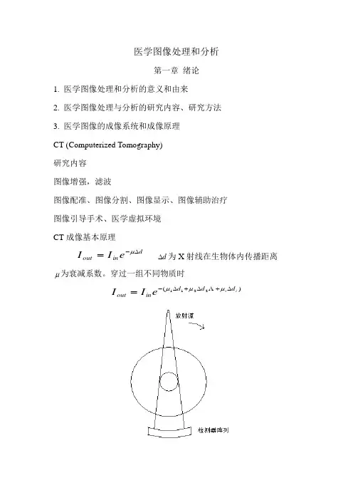
医学图像处理和分析第一章 绪论1. 医学图像处理和分析的意义和由来2. 医学图像处理与分析的研究内容、研究方法3. 医学图像的成像系统和成像原理 CT (Computerized Tomography) 研究内容 图像增强，滤波图像配准、图像分割、图像显示、图像辅助治疗 图像引导手术、医学虚拟环境 CT 成像基本原理d in oute I I ∆-=μd ∆为X 射线在生物体内传播距离μ为衰减系数。

穿过一组不同物质时)(2211i i d d d in out e I I ∆+∆+∆-=μμμCT原理示意图常用影像技术优缺点结构成像：X、CT、MRI、Ultrasound功能成像: f MRI、PET、SPECT1895年X射线机1969年英国工程师Hoopsfield设计成功第一台断层摄影装置CT 1972年应用于临床，获得第一幅脑肿瘤图像。

1979年Hoopsfield获诺贝尔奖螺旋CT 1987年出现于专利文献特点：数据无任何时间和空间间隔CT 连续两次扫描有一段间隔，螺旋CT没有，且空间分辨率更高。

MRI1946年Bloch and Purcell发现核磁共振NMR现象1952年获诺贝尔奖1973年第一幅核磁共振图像，纽约州立大学，两个充水式管1980年第一幅人体核磁共振图像。

1991年Ernst获诺贝尔化学奖在NMR中引入了Fourier变换超声成像光纤内窥镜成像。

MRA磁共振血管造影技术MagneticResonance Angiography正电子放射断层成像 PET (Position Emission Tomography) 单光子放射断层成像 SPECT (Single Photon Emission Computed Tomography)DSA 数字减影血管造影术 Digital Subtraction Angiography 参考书籍医学影像处理和分析, 田捷等编著, 电子工业出版社, 2003. 3D Imaging Medicine, J.K. Udupa, G .T. He4rman, CRC Press, 2000.第二章 图像的预处理1．直方图NN p ii =1,,1,0-=k i 110=∑-=k i ipN Nk i i=∑-=1直方图变换，拉伸和压缩)(r T s = )1,0(-∈L r线性变换⎪⎩⎪⎨⎧-+-+-+=322121121111)()()(tr r t r r t r t r r t r rt s 102211-≤<≤<≤≤L r r r r r r r321,,t t t 是变换系数直方图均衡化10<≤r(a) 在10<≤r ,)(r T 为单调增加 (b)例．假定一幅6464⨯．８个灰度级．分布如下．44.025.019.0)()()()(19.0)()()(1011100000=+=+=======∑∑==r p r p r p r T s r p r pr r T s r r j j r r j j2s =0.653s =0.81 4s =0.845s =0.956s =0.987s =1.00重新定义710≈s 731≈s 752≈s 763≈s 14≈s0s 790 1s 1023 2s 850 3s 985 4s 448总体 显示直方图统计，直方图均衡化，直方图分割滤波中值滤波高斯滤波参考文献：1.J. G. Liu, Y. Z. Liu, and G. Y. Wang, “Fast discrete W transforms via computat ionof moments”, IEEE Transactions on Signal Processing, vol. 53, no.2, pp.654-659, 2005.2.J. G. Liu, Y. Z. Liu, and G. Y. Wang, “Fast DCT-I, DCT-III, and DCT-IV viamoments”,EURASIP Applied Signal Processing, no.12, pp.1902-1909, 2005. 3.J. G. Liu, F. H. Y. Chan, F. K. Lam, H. F. Li, and George S. K. Fung,“Moment-based fast discrete Hartley transform”, Signal Processing, vol. 83, no. 8, pp. 1749-1757, 2003.4.J. G. Liu, F. H. Y. Chan, F. K. Lam, and H. F. Li, “Moment-based fast discretesine transforms”, IEEE Signal Processing Letters, vol. 7, no. 8, pp. 227-229, 2000.5.J. G. Liu, F. H. Y. Chan, F. K. Lam, and H. F. Li, “A novel approach to fastcalculation of moments of 3D gray level images”, Parallel Computing, vol. 26, no.6, pp. 805-815, 2000.6.J. G .Liu, H. F. Li, F. H. Y. Chan, and F. K. Lam, “A novel approach to fastdiscrete Fourier transform”, Journal of Parallel and Distributed computing, vol.54, pp. 48-58, 1998.7.J. G. Liu, H. F. Li, F. H. Y. Chan, and F. K. Lam, “Fast discrete cosine transformvia com putation of moments”, Journal of VLSI Signal Processing, vol. 19, no. 2, pp. 257-268, 1998.8.. F. H. Y. Chan, F. K. Lam, H. F. Li, and J. G. Liu, “An all adder systolic structurefor fast computation of moments”, Journal of VLSI Signal Processing, vol.12, no.2, pp. 159-175, 1996.矩和不变矩Since moment invariants were proposed by Hu in 1962, moment invariants, by virtue of invariance properties under translation, scaling and rotation, have played an important role in image analysis and pattern recognition. However, computing moment invariants directly is relatively expensive because of the large number of multiplications it requires and this weakness limits its extensive real-time applications. So fast computation of moment invariants has received considerable attention and many efforts have been made to solve it.Let f(x,y) be the image intensity function. The (p+q) order moments are defined aspq p q m x y f(x,y)dxdy =-∞+∞-∞+∞⎰⎰where p, q ∈{,,,...}012. Their discrete forms arem i j f pq p q i j j ni n===∑∑ 11where n n ⨯ is the image size and the size of a pixel is taken as the unit, f i j =f(i, j)The central moments of f(x, y) are defined asνpq p q x x y y f x y dxdy =---∞+∞-∞+∞⎰⎰()()(,) where x m m y m m ==10001000/,/ , with their discrete forms asνpq j ni n p q i i m m j m m f =--==∑∑(/)(/)1000110100 jThe central moment of order up to 3 are ,23 22 22 023 0 01202030301020201220112121102020102021*********2203030101011110000m y m y m m y m m x m y m x m m x m m y m x m y m m x m x m m y m m +-=-=+--=-=+--==+-==-==ννννννννννIn order to obtain moment invariants, transformation of the above moments is necessary,μνpq pq p q m =++/()/0012p, q={0, 1, 2, 3, ......} Seven functions of the second- and the third-order moments were first derived in 1961. These functions are known as Hu's moment invariants as follows,])()(3)[)(3( ])(3)()[()3())((4+ ])()()[(])()(3)[)(3(+ ])(3))[()(3()()()3()3(4)(221032301221033012203212123012300321721031230112032121230022062210323012210303212032121230123030125203212301242032121230321120220202201μμμμμμμμμμμμμμμμφμμμμμμμμμμμφμμμμμμμμμμμμμμμμφμμμμφμμμμφμμμφμμφ+-++-++-++-=+++-+-=+-++-+-++-=+++=-+-=++=+=They are invariant to image translation, rotation and scaling invariants and are expressed in terms of the ordinary moments m pq . In a direct computation of m pq , n 2 additions and n 2(p+q) multiplications are required. Obviously, for large values of n, the process will take a long time.Computation complexity O(n 2) .3. SYSTOLIC ARRAY FOR COMPUTING MOMENT INV ARIANTS We introduce the array generated the ordinary moments briefly here [2, 3].The p-network shown in Fig. 1 represents a map of transforming the vector (1, x, x 2, ...... x p-1, x p) into (1, (1+x), (1+x)2, ...... (1+x)p-1, (1+x)p). It is denoted by F p , i. e.F p (1, x, x 2, ...... x p-1, x p)=(1, (1+x), (1+x)2, ...... (1+x)p-1, (1+x)p)The equations below follow immediately.F p (1, 1, 1, ...... 1, 1)=(1, 2, 4, ......2p-1, 2p)F p (a, a, a, ...... a, a)=(a, 2a, 4a, ......2p-1a, 2pa)The equations below can then be verified by inputting data into the p-network.F p (a, ax, ax 2, ...... ax p-1, ax p)=(a, a(1+x), a(1+x)2, ...... a(1+x)p-1, a(1+x)p) F p (a+b, a+b, a+b, ...... a+b, a+b)=F p (a, a, a, ...... a, a)+F p (b, b, b, ...... b, b)F p2(1, x, x2, ...... x p-1, x p)=F p(F p(1, x, x2, ...... x p-1, x p))=F p(1, (1+x), (1+x)2, ...... (1+x)p-1, (1+x)p)=(1,(2+x), (2+x)2, ...... (2+x)p-1, (2+x)p)Fig. 1.The p-network.and in general,F p n-1(1, x, x2, ...... x p-1, x p)=F p(......F p(1, x, x2, ...... x p-1, x p)......)=(1, (n-1+x), (n-1+x)2, ...... (n-1+x)p-1, (n-1+x)p)By substitution,F p n-1(1, 1, 1, ......, 1, 1)=F p(......F p(1, 1, 1, ......, 1, 1)......)=(1, n, n2, ......, n p-1, n p)andF p n-1(a, a, a, ......, a, a)=(a, na, n2a, ......, n p-1a, n p a)Let a i=(a i, a i, a i,...... a i), i=1, 2, 3, ......, n, and a i is a (p+1)-dimensional vector, thenF p (F p (a n )+a n-1)=F p (F p (a n ))+F p (a n-1)=F p 2(a n )+F p (a n-1)Generally,F p (F p ......(F p (F p (F p (a n )+a n-1)+a n-2)+......a 2)+a 1=F p n-1(a n )+F p n-2(a n-1)+F p n-3(a n-1)+......+F p 2(a 3)+F p (a 2)+a 1=(, , ...... , , , 1112111i a ia i a i a a p ni i p ni in i i n i in i i∑∑∑∑∑=-====)The equation above can be proved by mathematical induction. These components of the resultant vector are known as 1-D moments. To compute these 1-D moments, F p is used (n-1) times in the iteration procedure except for the (n-1) additions of (p+1)-dimensional vectors.The ordinary moments of a discrete 2-D image, m pq (p, q = 0, 1, 2, .......), can be calculated by the following equation.m i j f jif pq pj n i n qij qj npi nij ======∑∑∑∑1111Let kj ki nij g if ==∑1( k=0, 1, 2, 3, ......, p, ......, )such that pq qpj j nm jg ==∑1It shows the computation of 2-D ordinary moments could be analyzed into two computation of 1-D moments .Without loss of generality, p ≥q is assumed. The systolic array for computing moments is shown in Fig. 2 [2, 3]. The systolic array consist of (n-1) p-network with someadders and proper feedbacks. In Fig. 2, data are pipelined from left to right at the speed of one cell per clock tick. At the same time, the correspondent input latches (denoted by squares in Fig.1) or adder-latches (denoted by circles) moved to their respective outputs. To retime the network, additional latches must be inserted between some nodes of the network. For simplicity, these latches are not explicitly drawn in Figure 2 but are represented by numbers enclosed in square brackets that are beside vertical and skew line.Fig. 2. The systolic array for computing the 2-D ordinary moments.By analyzing the schedule, the processing time for deriving all m r,s ( r=0, 1, 2, ......, p; s=0, 1, 2, ......q. ) is given byT=[(p+1)+(n-2)(p+1)]+1+[(q+1)+(n-1)(q+1)] =(p+q+2)nThe term [(p+1)+(n-2)(p+1)] is for calculating g 0,n , followed by a clock cycle to pass through the bridge cell, and the term [(q+1)+(n-1)(q+1)] is used in the second phase. Finally p cycles are needed to collect all the results. Altogether the number of additions performed is given by [(p+1)(p+2)(n-1)n/2+(q+1)(q+2)(n-1)(p+1)/2].在基于矩的算法中，要计算一种常系数的线性矩组合，算法中存余的浮点乘法就是常系数与矩的相乘，我们准备采用移位、累加方法将全部浮点乘法转化为定点整数加法。

医学图像的影像组学方法及其应用
目录
第1章绪论 1
1.1课题背景及意义 2
1.2研究现状 2
1.3本文主要研究内容2
第2章影像组学基础知识 4
2.1影像组学特征5
2.2特征降维 5
2.3模型 5
第3章胰腺癌预测过程及结果分析 4
3.1数据采集 5
3.2病灶勾画 5
3.3特征描述 5
3.4特征降维 5
3.5模型 5
3.6结果 5
第4章总结及展望 4
第1章绪论
1.1 课题背景及意义
目前，临床上的影像分析局限于医生对图像的主观判断，如分析病灶的形状、大小、位置、内部的均匀性及与周围正常组织的关系，仅仅是对CT密度、MRI 信号的灰度值的简单统计。

这种阅片方法依赖于医生的知识储备和临床经验，主观性和局限性较强，且简单的表面分析无法获得影像内部的深层次信息，容易造成误诊、漏诊的后果。

医学图像处理教案第一章：医学图像处理概述1.1 医学图像的类型与来源1.2 医学图像处理的重要性1.3 医学图像处理的基本流程1.4 医学图像处理的发展趋势第二章：医学图像处理基本原理2.1 图像数字化2.2 图像增强2.3 图像复原2.4 图像分割2.5 特征提取与表示第三章：医学图像处理方法3.1 灰度处理方法3.2 彩色处理方法3.3 形态学处理方法3.4 滤波处理方法3.5 机器学习与深度学习方法第四章：医学图像分析与应用4.1 医学图像分析概述4.2 医学图像配准4.3 医学图像重建4.4 医学图像分割在临床应用中的实例4.5 医学图像处理在科研中的应用第五章：医学图像处理软件与工具5.1 医学图像处理软件概述5.2 Photoshop医学图像处理应用实例5.3 MATLAB医学图像处理工具箱5.4 ITK医学图像处理软件库5.5 医学图像处理与分析在实际应用中的选择策略第六章：医学图像的预处理6.1 图像标准化6.2 图像归一化6.3 图像配准6.4 图像滤波6.5 图像预处理在医学图像分析中的应用第七章：图像增强技术7.1 图像增强的目的与方法7.2 直方图均衡化7.3 对比度增强7.4 锐化技术7.5 伪彩色增强7.6 图像增强算法的评估第八章：图像复原技术8.1 图像退化的模型8.2 线性滤波器8.3 非线性滤波器8.4 图像去噪8.5 图像去模糊8.6 图像复原技术的应用实例第九章：图像分割技术9.1 阈值分割9.2 区域增长9.3 边缘检测9.4 基于梯度的分割方法9.5 聚类分割9.6 图像分割的评价指标第十章：特征提取与表示10.1 特征提取的重要性10.2 基于几何的特征提取10.3 基于纹理的特征提取10.4 基于形状的特征提取10.5 特征选择与降维10.6 特征表示技术第十一章：医学图像配准技术11.1 图像配准的概念与意义11.2 基于互信息的图像配准11.3 基于特征的图像配准11.4 基于变换模型的图像配准11.5 医学图像配准的应用实例11.6 图像配准技术的评估与优化第十二章：医学图像重建技术12.1 图像重建的基本原理12.2 计算机断层扫描（CT）图像重建12.3 磁共振成像（MRI）图像重建12.4 正电子发射断层扫描（PET）图像重建12.5 单光子发射计算机断层扫描（SPECT）图像重建12.6 医学图像重建技术的应用与挑战第十三章：医学图像分割在临床应用中的实例分析13.1 胸部X光图像分割13.2 磁共振成像（MRI）脑部图像分割13.3 超声图像分割在腹部器官检测中的应用13.4 计算机断层扫描（CT）图像分割在肿瘤诊断中的应用13.5 医学图像分割在手术规划与导航中的应用第十四章：医学图像处理在科研中的应用案例分析14.1 医学图像处理在生物医学研究中的应用14.2 医学图像处理在药理学研究中的应用14.3 医学图像处理在神经科学研究中的应用14.4 医学图像处理在心脏病学研究中的应用14.5 医学图像处理在其他领域的研究应用第十五章：医学图像处理与分析的未来趋势15.1 与机器学习在医学图像处理中的应用15.2 深度学习技术在医学图像诊断与分析中的应用15.3 增强现实（AR）与虚拟现实（VR）在医学图像教学与培训中的应用15.4 云计算与大数据在医学图像处理与分析中的挑战与机遇15.5 跨学科研究与国际合作在医学图像处理领域的进展重点和难点解析重点：1. 医学图像的类型与来源，及其在医疗领域的重要性。

医学影像图像处理（课程）教学大纲「供成人医学影像学专升本（业余）专业使用」前言本课程教学大纲是按照成人高等教育医学影像学专升本（业余）专业培养方案编写。

本大纲供成人高等教育医学影像学专升本（业余）专业医学影像图像处理课程教学用,是对教学提出的基本要求。

其内容可通过讲课、实验或其他方式进行教学,讲授时不一定按此顺序，可根据情况作些调整。

本大纲既供教师备课使用,也供学生预习复习使用,以明确学习的基本要求及重点内容。

本课程教学目的是通过本课程的学习让学生掌握医学影像图像的开窗显示、线性灰度变换、空间变换、运算、滤波、锐化、分割、计算机辅助诊断、分子影像学、虚拟人体计划、二维和三维重建的基本原理。

熟悉各种医学影像图像处理软件的操作。

对医学影像图像处理的定义、研究内容、应用、研究现状、发展趋势、学习医学影像图像处理的意义有一个总体了解。

一、学时分配表：二、教学内容：第一章绪论第一节医学影像图像处理概论掌握：医学影像图像处理的研究内容和应用。

熟悉：医学影像图像的数据获取。

了解：医学影像图像处理的研究现状和发展趋势。

第二章医学影像图像的数据存放格式第一节DICOM标准的制定和应用掌握：DICOM标准的应用。

熟悉：DICOM标准制定的原因。

了解：DICOM标准发展的历史。

第二节DICOM标准的总体框架和主要内容掌握：DICOM标准的主要内容。

熟悉：DICOM标准的总体框架。

了解：DICOM标准的发展趋势。

第三节医学影像图像文件的存放格式掌握：DICOM文件格式和位图格式。

熟悉：JPEG格式。

了解：GI F、TIFF和PNG格式。

第三章医学影像图像的增强第一节医学影像图像的灰度变换掌握：医学影像图像处理的线性和非线性灰度变换。

熟悉：医学影像图像的开窗显示。

了解：医学影像图像灰度变换的应用。

第二节医学影像图像的灰度直方图掌握：医学影像图像灰度直方图均衡。

熟悉：医学影像图像灰度直方图的获得。

了解：医学影像图像灰度直方图的应用。