Erratum to Deformation Quantization in Algebraic Geometry

Teor Imov r.ta Matem.Statist.Theor.Probability and Math.Statist. Vip.75,2006No.75,2007,Pages189–199S0094-9000(08)00725-4Article electronically published on January25,2008ASYMPTOTIC QUANTIZATION ERRORSFOR UNBOUNDED QUANTIZERSUDC519.21M.SHYKULAAbstract.We consider non-uniform scalar quantization for a wide class of un-bounded random variables(or values of a random process sampled in time).As-ymptotic stochastic structures for quantization errors are derived for two types ofquantizers when the number of quantization levels tends to infinity.The correspond-ing results for bounded random variables are generalized.Some numerical examplesillustrate the rate of convergence.1.IntroductionQuantization of continuous random signals(or random variables and processes)is an important part of digital representation of analog signals for various coding techniques (e.g.,source coding,data compression,archiving,restoration).Quantization aims at representing a realization of a continuous in value and/or time random process(or sig-nal)by afinite-dimensional vector.The most comprehensive overview of quantization problems can be found in[6](for later references,see[5]).A quantizer introduces some distortion into the data and the problem of evaluation of this distortion arises.A number of authors estimate distortion measures for quantizers(see,e.g.,[14]and[8]).A class of asymptotically optimal quantizers with respect to an r th-mean error distortion measure is considered in[4](see also[3,13]).A different approach for uniform scalar quantization is developed in[12],where the correlation properties of a Gaussian process are exploited to evaluate the asymptotic behavior of the random quantization rate for uniform quantizers. General quantization problems for Gaussian processes in infinite-dimensional functional spaces are considered in[10].Mapping of a realization of a continuous in value and/or time process into afinite-dimensional vector requires both discretization in time(or sampling)and amplitude(or quantization).The problems of optimal sampling for spline approximation are studied in[11].We consider quantization of a random variable,which is the value of a random process at afixed sampling point.In this paper we derive the stochastic structure of the asymptotic quantization error for a general class of quantizers when the number of quantization levels tends to infinity.Let X be a continuous random variable with a density function f(x),x∈R.Following Bennett’s notations(see[1]),the N-level companding quantizer(also called compander)Q N,G(x)is defined asQ N,G(x)=G−1Q N,U(G(x)),(1)2000Mathematics Subject Classification.Primary60G99;Secondary94A29,94A34.Key words and phrases.Non-uniform scalar quantization,random process,stochastic structure.c 2008American Mathematical Society189190M.SHYKULAwhere G :R →(0,1)is onto and increasing,and Q N,U is the N -level uniform quantizer on (0,1),Q N,U (y )= n N −12N if y ∈ n −1N ,n N ,n =1,...,N −1,1−12N if y ∈ N −1N ,1 .(2)Note that the inverse function S :=G −1of G provides a transformation from a uni-form quantization to a non-uniform one.The quantization intervals of the companding quantizer Q N,G ,I 1,N = −∞,S 1N ,I n,N = S n −1N ,S n N,n =2,...,N −1,and I N,N = S N −1N,∞ ,and the corresponding quantization levels,u n,N =S n N −12N,n =1,...,N,set up a design D N =D N,G ,N ≥1.Let g (x )define the probability density function corresponding to G (x ),i.e.,G (x )= x −∞g (v )dv ,x ∈R .We call g (x )the quantization density function .In what follows we consider a sequence of regular designsD N (g )=D N,G (g ),N ≥1,generated by a positive continuous g (x ),x ∈R , S (n/N )−∞g (x )dx =n N ,n =1,...,N −1,and S (n/N −1/(2N ))−∞g (x )dx =n N −12N ,n =1,...,N.Note that g (x )characterizes the distribution of quantization levels.It follows from (1)that G (x )provides a transformation from a non-uniform quantization of the random variable X to a uniform quantization of a random variable G (X )with values in (0,1),i.e.,G (Q N,G (x ))=Q N,U (G (x )).Henceforth,let d →denote convergence in distribution.Some problems on asymptotically optimal companding quantization are discussedin [1].For example,for the r th-mean error distortion measureD (Q N,G (X ))=E |X −Q N,G (X )|r ,r >0,it is shown in [1]thatlim N →∞N r D (Q N,G (X ))=1(r +1)2r R f (x )g (x )rdx =C r >0.(3)It follows by H¨o lder’s inequalitythat the right-hand side of (3)is minimal if and only if g (x )=f (x )1/(r +1) R f (z )1/(r +1)dz (cf.[3]).For a random variable X with values in a finite interval,the stochastic structure of the asymptotic normalized quantization errorand asymptotic properties of the corresponding additive noise non-uniform quantization model are derived in [13].Probability densities of the asymptotic vector quantization errors are studied in [7].In our paper we obtain the stochastic structure of the asymptotic non-uniform scalar quantization errors for a random variable when the support of the density is not necessarily finite (unbounded quantizer).ASYMPTOTIC QUANTIZATION ERRORS FOR UNBOUNDED QUANTIZERS 191The paper is organized as follows.In Section 2we consider two types of non-uniform scalar quantizers.For these quantizers we find the stochastic structures of asymptotic normalized errors for non-uniform quantization of random variables.Section 3provides some examples and numerical experiments to illustrate the rate of convergence in the obtained results.In Section 4proofs of the statements in the previous sections are given.2.ResultsIn this section we consider the stochastic structure of the asymptotic quantization error for two non-uniform companding quantizers.For a random variable with values in a finite interval the stochastic structure of non-uniform quantization error is derived in [13]asymptotically when the number of quantization levels tends to infinity.Hence-forth,let X be a continuous random variable with density function f (x ),x ∈R ,not necessarily with bounded support.Let g (x )be a quantization density function.From now on we assume that the density functions f (x )and g (x )have the same support.Various conditions on the density functions of quantized random variables and quantiza-tion density functions are considered in a number of quantization papers,mostly in the applied literature (see,e.g.,[7]).We introduce the following conditions on f (x )and g (x ):(A 1)The quantization density function g (x ),x ∈R ,is positive and uniformly contin-uous.(A 2)There exists C >0such that f (x )≤Cg (x )for every x ∈R .(A 3)The density function f (x ),x ∈R ,is continuous.For example,the assumptions (A 1)–(A 3)hold if the density functions f (x )and g (x )are Gaussian with identical parameters.Let G (x )be a distribution function corresponding to g (x ).For X and G (x )recall that Q N,G (X )denotes the N -level companding quantizer with quantization designD N =D N (g ),N ≥1(cf.(1)).In the following theorem,the stochastic structure of the normalized non-uniform quantization error Z N,G (X )=N (X −Q N,G (X ))is derived asymptotically as N →∞.Let U be a random variable uniformly distributed on [−1/2,1/2].Theorem 1.Let X be a continuous random variable with density function f (x ),x ∈R .Let g (x )be a quantization density function and Q N,G (X )the non-uniform companding quantizer.If (A 1)and (A 2)hold,then(i)g (X )Z N,G (X )d→U as N →∞;(ii)Z N,G (X )d →U/g (X )as N →∞,where X and U are independent random variables.Remark 1.In particular,this result is valid for random variables with values in a finite interval (cf.[13]).Various quantization methods are used in quantization applications and theory.Now we consider a quantizer Q N,G with the same quantization intervals as for Q N,G ,I n,N ,n =1,...,N ,but with quantization levels in the middle of the intervals,except for the intervals I 1,N and I N,N ,where the levels do not change,i.e.,Q N,G (x )=⎧⎪⎨⎪⎩S 12N if x ∈I 1,N ,12 S n N +S n −1N if x ∈I n,N ,n =2,...,N −1,S 2N −12Nif x ∈I N,N (cf.[3]).Further,for a random variable X we use the result from [9]demonstrating the asymptotic equivalence of the non-uniform quantizers Q N,G (X )and Q N,G (X )with192M.SHYKULArespect to the r th-mean error distortion measure D (Q N,G )=E |X −Q N,G (X )|r ,r >0,N ≥1.For X with density function f (x )let p (y )denote the probability density function of the random variable Y :=G (X ),p (y )=f (S (y ))/g (S (y )),y ∈[0,1].Recall that S is the inverse function of G .In particular,the assumption (A 2)corresponds to boundedness of the density p (y ).As in [9]we introduce the following sufficient conditions on f (x )and g (x )for the validity of (3):(B 1)g (x )is positive and continuous.(B 2)There exists M >0such that g (x )is increasing if x <−M and g (x )is decreasingif x >M .(B 3) R f (x )/g (x )r dx <∞for some r >0.(B 4)For some ε>0 εs (x/2)r p (x )dx <∞and 11−εs ((x +1)/2)r p (x )dx <∞,where,by definition,s (y )=S (1)(y ),y ∈(0,1)(see also [2]for some different sufficient conditions on f (x )and g (x )).The assumption (B 1)together with the tail conditions in (B 4)is somewhat similar to (A 1).Under the assumptions (B 1)–(B 4),it is shown in [9]that the r th-mean quanti-zation errors for N -level non-uniform quantizers Q N,G and Q N,G have the same behavior asymptotically as N →∞,lim N →∞N r D (Q N,G )=lim N →∞N r D (Q N,G )=C r >0(4)(cf.(3)).This result justifies the application of the quantizer Q N,G ,at least with respect to the r th-mean distortion measure.Moreover,in the following theorem we show that for a random variable X the asymptotic normalized quantization errorsZ N,G (X )=N (X −Q N,G (X ))and Z N,G (X )=N (X −Q N,G (X ))have identical stochastic structure as N →∞under the assumptions (A 1)–(A 3).Theorem 2.Let X be a continuous random variable with density function f (x ),x ∈R .Let g (x )be a quantization density function and Q N,G (X )the non-uniform quantizer.If (A 1)–(A 3)hold,then(i)g (X )Z N,G (X )d→U as N →∞.(ii)Z N,G (X )d →U/g (X )as N →∞,where X and U are independent random variables.Remark 2.Theorems 1(ii)and 2(ii)correspond to the asymptotic result (3).In fact,E (U/g (X ))r =C r .These results can be applied when various asymptotic properties of quantization errors are investigated.3.Numerical examples and simulationsThe following numerical examples illustrate the rate of convergence in distribution for Theorems 1and 2from Section 2.In this section,the quantizers Q N,G and Q N,G are said to be Quantizer 1and 2,respectively.We approximate the distribution functions in the examples below by the corresponding empirical distribution functions.Denote by F V (x )the distribution function of a random variable V .Recall that N denotes the number of quantization levels.Let N s denote the number of simulations.ASYMPTOTIC QUANTIZATION ERRORS FOR UNBOUNDED QUANTIZERS 193Example 1.Let X 1be a standard Gaussian variable.Let g 1(x )be a standard Gaussianquantization density function.The assumptions (A 1)–(A 3)hold and we rewrite Theorems 1(i)and 2(i)in the following form:F g 1(X 1)Z N,G 1(X 1)(x )→x +1/2as N →∞(5)for Quantizer 1andF g 1(X 1)Z N,G 1(X 1)(x )→x +1/2as N →∞(6)for Quantizer 2,where G 1(x )is the distribution function corresponding to the den-sity g 1(x ).Figures 1and 2illustrate the rate of convergence in (5)and (6),respectively.Figure 1.The empirical distribution functions F g 1(X 1)Z N,G 1(X 1)(x )(Quantizer 1)for N =3(dashed )and N =20(solid ),and the uni-form distribution function F U (x )=x +1/2(stars );N s =50000.Example 2.Let X 2be a Gaussian variable with zero mean and standard deviation 3.Let g 2(x )be a quantization density function of the Cauchy distribution with parameters 0and 1.The assumptions (A 1)–(A 3)hold and we rewrite Theorems 1(ii)and 2(ii)in the following form:F Z N,G 2(X 2)(x )→F U/g 2(X 2)(x )as N →∞(7)for Quantizer 1and1F Z N,G 2(X 2)(x )→F U/g 2(X 2)(x )as N →∞(8)for Quantizer 2,where G 2(x )corresponds to g 2(x ).Figures 3and 4illustrate the rate of convergence in (7)and (8),respectively.194M.SHYKULAFigure 2.The empirical distribution functions F g1(X1)Z N,G1(X1)(x)(Quantizer2)for N=3(dashed)andN=20(solid),andtheuni-formdistribution functionFU(x)=x+1/2(stars);N s=50000.Figure 3.The empirical distribution functions F Z N,G2(X2)(x)(Quan-tizer1)for N=2.25(solid),and F U/g2(X2)(x)(dashed);N s=50000.ASYMPTOTIC QUANTIZATION ERRORS FOR UNBOUNDED QUANTIZERS195Figure 4.The empirical distribution functions F Z N,G 2(X 2)(x )(Quan-tizer 2)for N =2.25(solid ),and F U/g 2(X 2)(x )(dashed );N s =50000.4.ProofsHenceforth,let φV (v )denote the characteristic function of a random variable V .Proof of Theorem 1.We begin with (ii).For the random variable Y =G (X )with values in (0,1),we have the uniform N -level scalar quantizerQ N,U (Y )=Q N,U (G (X ))=G (Q N,G (X ))(cf.(1)and (2)),and the normalized quantization error Z N,U (Y )=N (Y −Q N,U (Y )).Note that the function G (x )is increasing and continuously differentiable,G (1)(x )=g (x ),x ∈R .Thus the inverse function S of G is also continuously differentiable andS (1)(y )=1g (S (y )),y ∈(0,1).(9)By the mean value theorem,there exists X N between X and Q N,G (X )such thatZ N,U (Y )=N (G (X )−G (Q N,G (X )))=g (X N )Z N,G (X ).We getZ N,G (X )= 1+g (X N )−g (X )g (X ) −1Z N,U (Y )g (X ).Further,uniform continuity of g (x )(the assumption (A 1))implies that(g (X N )−g (X ))/g (X )→0as N →∞(a.s.).Thus it follows by the Cram´e r–Slutsky Theorem thatZ N,G (X )d →U/g (X )as N →∞sinceZ N,U (Y )/g (X )d →U/g (X )as N →∞,(10)196M.SHYKULAX =S (Y ).In order to prove (10),we show that φZ N,U (Y )/g (S (Y ))(v )→φU/g (S (Y ))(v )as N →∞,v ∈R .(11)By the definition (2),for the density function p (y )of the random variable Y ,we have φZ N,U (Y )/g (S (Y ))(v )=10exp ivN (y −Q N,U (y ))/g (S (y )) p (y )dy =N n =1 n/N (n −1)/Nexp ivN y − n N −12N g (S (y )) p (y )dy =N n =1 n/N −1/(2N )(n −1)/Nexp ivN y − n N −12N g (S (y )) p (y )dy +N n =1 n/N n/N −1/(2N )exp ivN y − n N −12N g (S (y )) p (y )dy =S 1(N )+S 2(N ).(12)Consider the sum S 1(N ).We getS 1(N )=N n =1 n/N −1/(2N )(n −1)/Nexp ivN y − n N −12N g (S (y )) p (y )dy = 0−1/2 N n =1exp ivz g S 1N n −12 +z N ×p (n −1/2)N −1+zN −1 N −1 dz,by changing the variable,z =N (y −N −1(n −1/2)).It follows from (A 2)that there exists C >0such thatp (y )=f (S (y ))/g (S (y ))≤C,and we get N n =1exp ivz g S 1N n −12 +z N p (n −1/2)N −1+zN −1 N −1 ≤C.Hence,by the dominated convergence theorem and elementary properties of the Riemann integral,S 1(N )→ 0−1/2 1e ivz/g (S (y ))p (y )dy dz as N →∞.(13)Similarly as for S 1(N ),we have S 2(N )→1/2010e ivz/g (S (y ))p (y )dy dz as N →∞.(14)Now (12)together with (13)and (14)implies φZ N,U (Y )/g (S (Y ))(v )→ 1/2−1/2 1e ivz/g (S (y ))p (y )dy dz =φU/g (S (Y ))(v )as N →∞and S (Y )=X and U are independent random variables.Hence (11)holds.This completes the proof of the assertion (ii).The idea of the proof of (i)is the same as in the proof of (ii).Notice thatQ N,G (X )=S (Q N,U (Y )),X =S (Y ).ASYMPTOTIC QUANTIZATION ERRORS FOR UNBOUNDED QUANTIZERS 197Thusg (X )Z N,G (X )=Ng (X )(X −Q N,G (X ))=Ng (S (Y )) S (Y )−S (Q N,U (Y )) .(15)Furthermore,it follows by the mean value theorem and (9)that there exists Y N be-tween Y and Q N,U (Y )such that S (Y )−S (Q N,U (Y ))=(Y −Q N,U (Y ))/g (S (Y N )).Therefore,combining (A 1)with the Cram´e r–Slutsky Theorem applied to (15)and using that g (S (Y N ))→g (S (Y ))(a.s.)as N →∞for |Y N −Y |≤|Q N,U (Y )−Y |≤1/N ,we getg (X )Z N,G (X )=g (S (Y ))g (S (Y N ))Z N,U (Y )d →U as N →∞.In order to prove the assertion (i),it is enough to show thatZ N,U (Y )d →Uas N →∞or equivalentlyφZ N,U (Y )(v )→φU (v )as N →∞,v ∈R .(16)But (16)can be proved in the same way as in the proof of (11).Hence (i)holds.This completes the proof of the theorem. Proof of Theorem 2.First we prove (ii).By the definition we haveZ N,G (X )=Z N,G (X )+d N (X ),(17)where d N (X )=d N,G (X ):=N (Q N,G (X )−Q N,G (X )),N ≥1.Therefore,in view of the Cram´e r–Slutsky Theorem,to prove the assertion of the theorem it is enough to showthat d N (X )d →0or,equivalently,φd N (X )(v )→1as N →∞(18)since,by Theorem 1,Z N,G (X )d →U/g (X )as N →∞.Observe that by the definitionsφd N (X )(v )=E e ivd N (X )=N −1 n =2 S (n/N )S ((n −1)/N )exp ivN S n N −12N −12 S n N +S n −1Nf (x )dx.(19)To prove (18)we estimate φd N (X )(v )−1 by splitting up the sum in (19).For a givenδ>0,select a sufficiently small a 0=a 0(δ)>0such thatI 2(a 0):= a 00p (y )dy + 11−a 0p (y )dy <δ.(20)We represent φd N (X )(v )as follows:φd N (X )(v )=S 1,N (a 0)+S 2,N (a 0),1=I 1(a 0)+I 2(a 0),198M.SHYKULAwhereS 1,N (a 0):=2≤n ≤N −1:n/N ∈[a 0,1−a 0]exp iv N 2 S n N −12N −S n −1N + S n N −12N −S n N×S (n/N )S ((n −1)/N )f (x )dx.Further,combining the mean value theorem with (A 3)and (9),we get S 1,N (a 0)= 2≤n ≤N −1:n/N ∈[a 0,1−a 0]exp i v 4 1g (S (ν n ))−1g (S (ν n )) ×f (S (ω n ))1g (S (ω n))1N (21)for someν n ,ν n ,ω n ,ω n ∈[(n −1)/N,n/N ],n =2,...,N −1.We use the following elementary property of the Riemann integral:if two functions h (x )and ϕ(x )are Riemann integrable on [a,b ]⊂R ,thenlim max |∆x i |→0n −1 i =0h (ξi )ϕ(θi )∆x i = b ah (x )ϕ(x )dx,(22)wherex i ≤ξi ,θi ≤x i +1,∆x i =x i +1−x i ,i =0,1,...,n −1(a =x 0<x 1<x 2<···<x n =b ),n ≥1.This property can be generalized to any finite number of Riemann integrable functions.Thus (22)applied to functions exp i v 4 1g (S (y ))−1g (S (y )),f (S (y )),and 1/g (S (y ))in (21)implies thatS 1,N (a 0)→ 1−a 0a 0f (S (y ))g (S (y ))dy =I 1(a 0)as N →∞.HenceS 1,N (a 0)−I 1(a 0) <δ(23)for a sufficiently large N .We have also that |S 2,N (a 0)|≤2≤n ≤N −1:n/N ∈[0,1]\[a 0,1−a 0] S (n/N )S ((n −1)/N )f (x )dx ≤S (a 0)−∞f (x )dx + ∞S (1−a 0−1/N )f (x )dx = a 00p (y )dy +11−a 0−1/N p (y )dy <2δ(24)ASYMPTOTIC QUANTIZATION ERRORS FOR UNBOUNDED QUANTIZERS199 for a sufficiently large N,by changing the variable y=G(x).Applying(20),(23), and(24),we obtainφdN (X)(v)−1≤S1,N(a0)−I1(a0)+S2,N(a0)+I2(a0)<4δfor a sufficiently large N.Sinceδ>0is arbitrary,(18)ing a similar technique as in the proof of(ii)and taking into account(17),Theorem1(i),and(18),we immediately get the assertion(i).This completes the proof. Acknowledgments.The author is grateful to Associate Professor Oleg Seleznjev for many fruitful discussions and suggestions during the work.Bibliography1.W.R.Bennett,Spectrum of quantized signal,Bell.Syst.Tech.J.27(1948),446–472.MR0026287(10:133f)2.J.A.Bucklew and G.L.Wise,Multidimensional asymptotic quantization theory with r th powerdistortion measures,IEEE rm.Theory28(1982),239–247.MR651819(83b:94026)3.S.Cambanis and N.Gerr,A simple class of asymptotically optimal quantizers,IEEE Trans.Inform.Theory29(1983),664–676.MR730904(85a:94001)4.S.Graf and H.Luschgy,Foundations of Quantization for Probability Distributions,Springer-Verlag,New York,2000.MR1764176(2001m:60043)5.R.M.Gray and T.Linder,Mismatch in high rate entropy constrained vector quantization,IEEE rm.Theory49(2003),1204–1217.MR1984821(2004e:94026)6.R.M.Gray and D.L.Neuhoff,Quantization,IEEE rm.Theory44(1998),2325–2383.MR1658787(99i:94029)7. D.H.Lee and D.L.Neuhoff,Asymptotic distribution of the errors in scalar and vector quan-tizers,IEEE rm.Theory42(1996),446–460.8.J.Li,N.Chaddha,and R.M.Gray,Asymptotic performance of vector quantizers with a per-ceptual distortion measure,IEEE rm.Theory45(1999),1082–1091.MR1686244 (2000b:94008)9.T.Linder,On asymptotically optimal companding quantization,rm.Theory20(1991),475–484.10.H.Luschgy and G.Pag`e s,Functional quantization of Gaussian processes,Jour.Func.Annal.196(2002),486–531.MR1943099(2003i:60006)11.O.Seleznjev,Spline approximation of random processes and design problems,Jour.Stat.Plan.Infer.84(2000),249–262.MR1747507(2001e:62082)12.M.Shykula and O.Seleznjev,Uniform quantization of random processes,Univ.Ume˚a ResearchReport1(2004),1–16.13.M.Shykula and O.Seleznjev,Stochastic structure of asymptotic quantization errors,Stat.Prob.Letters76(2006),453–464.MR226659814.P.L.Zador,Asymptotic quantization error of continuous signals and the quantization dimen-sions,IEEE rm.Theory28(1982),139–148.MR651809(83b:94014)Department of Mathematics and Mathematical Statistics,Ume˚a University,SE-90187 Ume˚a,SwedenE-mail address:mykola.shykula@math.umu.seReceived24/JUL/2005Originally published in English。

《孟德尔随机化研究指南》中英文版English:"Mendelian randomization (MR) has emerged as an important tool in epidemiology and biostatistics for investigating causal relationships between risk factors and disease outcomes. In order to ensure the validity and reliability of MR studies, researchers need to follow a standardized set of guidelines. The 'Mendelian Randomization Reporting Guidelines (MR-REWG)' provide detailed recommendations for conducting, reporting, and appraising MR studies. These guidelines cover key aspects such as study design, instrument selection, data sources, statistical analysis, and result interpretation. By adhering to these guidelines, researchers can minimize bias and confounding, and produce more robust evidence for causal inference in epidemiological research."中文翻译:“孟德尔随机化（MR）已经成为流行病学和生物统计学中研究危险因素与疾病结果之间因果关系的重要工具。

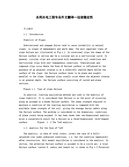
水利水电工程专业外文翻译--边坡稳定性外文翻译1.1 IntroductionStability of SlopesGravitational and seepage forces tend to cause instability in natural slopes, in slopes of embankments and earth dams. The most important types of slope failure arc illustrated in Fig.1.1. In rotational slips the shape of the failure surface in section may be a circular are or a non-circular curve. In general, circular slips are associated with homogeneous soil conditions and non-circular slips with non- homogeneous conditions. Translational and compound slips occur where the form of failure surface is influenced by the presence of an adjacent stratum is at a relatively shallow depth bellow the surface of the slope: the failure surface tends to be plane and roughly parallel to the slope. Compound slips usually occur where the adjacent stratum is at greater depth, the failure surface consisting of curved and plane sections.Figure 1.1 Type of slope failureIn practice, limiting equilibrium methods are used in the analysis of slope stability. It is considered that failure is on the point of occurring along an assumed or a known failure surface. The shear strength required to maintain a condition of the limiting equilibrium is compared with theavailable shear strength of the soil, giving the average factor safety along the failure surface. The problem is considered in two dimensions, conditions of plane strain being assumed. It has been shown that two-dimensional analysis gives a conservative result for a failure on a three-dimensional (dish-shaped) surface. Figure 1. 2 The ?u=0 analysis1.2 Analysis for the Case of ?u=0The analysis, in term of total stress ,covers the case of a fully-saturated clay under undrained conditions, i.e. for the condition immediately after construction. Only moment equilibrium is considered in the analysis. In section, the potential failure surface is assumed to be a circle arc. A trial failure surface (centre O, radius and length La) is shown in Fig 1.2.Potentialinstability is due to the total weight of the soil mass(W per unit length) above the failure surface. For equilibrium the shear strength which must be mobilized along the failure surface is expressed as: ?m=?fCu= FFwhere F is the factor of safety with respect to shear strength. Equation moment1about O:CuLar FCuLar F= (1.1)Wd Wd=The moments of any additional forces must be taken into account. In the event of a tension crack developing, as shown in Fig1.2,the arc length La is shortened and a hydrostatic force will act normal to the crack if the crack fills with water. It is necessary to analyze the slope for a number of trial failure surfaces in order that the minimum factor of safety can be determined.Example 1.1A 45°slope i s excavated to a depth of 8m in a deep layer of unit weight 19kN/m3: the relevant shear strength parameters are cu=65kN/m3and ?u=0.Determine the factor of safety for the trial surface specified in Fig1.3. In Fig1.3, the cross-sectional area ABCD is 70m2. The weight of the soil mass=70×19=1330m2. The cent roid of ABCD is 4.5m from O.The angle AOC is 89.5°and radius OC is 12.1m.The arc length ABC is calculated as 18.9m. The factor of safety is given by:CuLar Wd65?18.9?12.165?18.9?12.1 =1330?4.51330?4.5 F==2.48This is the factor of safety for the trial failure surface selected and is notnecessarily the minimum factor of safety.Figure 1.3 example 1.11.3 The ?-Circle MethodThe analysis is in terms of total stress. A trial failure surface , acircular arc (centre o, radius r) is selected as shown in Fig 1.4.If the shearstrength parameters are cu and ?u ,the shear strength which must be mobilizedfor equilibrium is: ?m=?f=?l F =cm+?tan?mFigure 1.4 The ?-circle method2Where F is the factor of safety with respect to shear strength .Forconvenience the following notation is introduced: cm=cu (1.2) Fc tan?m=tan?u (1.3) F?it being a requirement that: FC=F?=FAn element ab, of length l, of the failure surface is considered, theelement being short enough to be approximated to a straight line. The forcesacting on ab (per unit dimension normal to the section) are as follows: (1)the total normal force ?1;(2) the component of shearing resistance cml;(3) the component of shearing resistance ?1tan?m.If each force cml along the failure surface is split into componentsperpendicular and parallel to the chord AB, the perpendicular components sumto zero and the sum of the parallel components is given by:C=cmLc (1.4)where Lc is the chord length AB. The force C is thus the resultant, actingparallel to the chord cml. The line of application of the resultant force Ccan be determined by taking moments about the centre O, then: C rc=r?cml i.e.cmLcrc=rcmLa where La=?l is the arc length AB. Thus,rc=Lar (1.5) LCThe resultant of the forces ?1and ?1tan?m on the element ab acts at angle ?m to the normal and is the force tangential to a circle, centre O, of radius r sin?m: this circle is referredto as the ?-circle. The same technique was used in Chapter 5.The overallresult (R) for the arc AB is assumed to be tangential to the ?-circle. Strictly, the resultant R is tangential to a circle of radius slightly greater than r sin?mbut the error involved in the above assumption is generally insignificant.The soil mass above the trial failure surface is in equilibrium under itstotal3weight (W) and the shear resultants C and R. The force W is known in magnitude and direction; the direction only of the resultant C is known.Initially a trial value of F? is selected and the corresponding value of ?m is calculated from equation 1.3.For equilibrium the line of application of the resultant R must be tangential to the ?-circle and pass though the point of intersection of the forces W and C. The force diagram can then be drawn, from which the value of C can be obtained .Then:cm =andFC=Cu CmC LCIt is necessary to repeat the analysis at least three times,starting with different values of F?.If the calculated values of FC areplotted against the corresponding values of F?,the factor of safetycorresponding to the requirement FC=F? can be determined .The whole procedure must be repeated for a series of trial failure surfaces in order that the minimum factor of safety is obtained.For an effective stress analysis the total weight W is combined with the resultant boundary water force on the failure mass and the effective stress parameters c′and ?′used.Based on the principle of geometric similarity, Taylor（1.13）published stability coefficients for the analysis of homogeneous slopes in terms of total stress. For a slope of height H the stability coefficients for the analysis of homogeneous slopes in terms of total stress. For a slope of height H the stability coefficient (Ns) for the failure surface along which thefactor of safety is a minimum is:Ns=Cu (1.6) F?HValues of Ns , which is a function of the slope angle ? and the shear strength parameter ?u,can be obtained from Fig 1.5.For ?u=0,the value of Ns also depends on the depthfactor D, where DH is the depth to a firm stratum. Firm stratumFigure 1.5 Taylor′s coefficients.In example 1.1, ?=45°, ?u=0,and assuming D is large, the value of Ns is 0.18.Then from equation 1.6:4F= =Cu Ns?H650.18?19?8 =2.37Gibson and Morgenstern〔1.4〕published stability coefficients for slopes in normally-consolidated clays in which the untrained strength cu(?u=0) varies linearly with depth.Figure 1.6 Example 1.2Example 1.2An embankment slope is detailed in Figure 1.6.Fir the given failure surface. Determine the factor of safety in terms of total stress using the ?-circle method. The appropriate shear strength parameters are cu=15kN/m2and ?u=15°: the unit weight of soil is 20 kN/m2.The area ABCD is 68 m2 and the centroid (G) is 0.60m from the vertical through D. The radius of the failure arc is 11.10m.The arc length AC is 19.15 m and the chord length AC is 16.85m. The weight of the soil mass is:W=68×20=1360 k N/m Th e position of the resultant C is given by:Lar LC19.15= ×11.1016.85r c=Now:?m=tan-1(tan15) F?Trial value of F? are chosen, the corresponding values of rsin ?m are calculated and the ?-circle drawn shown in Fig.1.6.The resultantC(for any value of F?) acts in a directions parallel to the chord AC and at distance rc from O. The resultant C(for any value F?) acts in a direction parallel to the chord AC and at distance rc from O. The forces C and W intersect at point E. The resultant R, corresponding to each value of F?, passes through E is tangential to the appropriate ?-circle. The force diagrams are drawn and the values of C determined.5感谢您的阅读，祝您生活愉快。

《孟德尔随机化研究指南》中英文版全文共3篇示例，供读者参考篇1Mendel's Randomization Research GuideIntroductionMendel's Randomization Research Guide is a comprehensive resource for researchers in the field of genetics who are interested in incorporating randomization into their study designs. Developed by Dr. Gregor Mendel, a renowned geneticist known for his pioneering work on the inheritance of traits in pea plants, this guide provides a detailed overview of the principles and methods of randomization in research.Key ConceptsRandomization is a crucial tool in scientific research that helps to eliminate bias and increase the validity of study findings. By randomly assigning participants to different treatment groups or conditions, researchers can ensure that the groups are comparable and that any observed differences are truly due to the intervention being studied.The guide covers a range of topics related to randomization, including the importance of random assignment, the different types of randomization methods, and the potential pitfalls to avoid when implementing randomization in a study. It also provides practical guidance on how to design and conduct randomized experiments, including tips on sample size calculation, randomization procedures, and data analysis methods.Benefits of RandomizationRandomization offers several key benefits for researchers, including:1. Increased internal validity: Random assignment helps to ensure that the groups being compared are equivalent at the outset of the study, reducing the risk of confounding variables influencing the results.2. Improved generalizability: By minimizing bias and increasing the reliability of study findings, randomization enhances the external validity of research findings and allows for more generalizable conclusions to be drawn.3. Ethical considerations: Randomization is considered a fair and unbiased method for allocating participants to differentgroups, helping to ensure that all participants have an equal chance of receiving the intervention being studied.Practical ApplicationsThe guide provides practical examples of how randomization can be applied in research studies, ranging from clinical trials to observational studies. For example, researchers conducting a randomized controlled trial may usecomputer-generated randomization software to assign participants to different treatment groups, while researchers conducting an observational study may use stratified random sampling to ensure that key variables are evenly distributed across study groups.In addition, the guide outlines best practices for implementing randomization in research studies, including the importance of blinding participants and investigators to group assignment, documenting the randomization process, and conducting sensitivity analyses to assess the robustness of study findings.ConclusionIn conclusion, Mendel's Randomization Research Guide is an invaluable resource for researchers seeking to incorporaterandomization into their study designs. By following the principles and methods outlined in the guide, researchers can enhance the validity and reliability of their research findings, ultimately leading to more impactful and meaningful contributions to the field of genetics.篇2Mendel Randomization Research GuideIntroduction:The Mendel randomization research guide is a comprehensive manual that provides researchers with detailed instructions on using Mendelian randomization (MR) in their studies. MR is a statistical method that uses genetic information to investigate causal relationships between exposures, known as risk factors, and outcomes, such as diseases or health-related outcomes. This guide aims to help researchers understand the principles of MR, design robust studies, and interpret their results accurately.Key Sections:1. Introduction to Mendelian Randomization:- Overview of MR as a method for assessing causality- Explanation of the assumptions underlying MR studies- Discussion of the advantages and limitations of MR compared to traditional observational studies2. Study Design:- Selection of genetic instruments for exposure variables- Matching of genetic instruments to outcome variables- Consideration of potential biases and confounding factors- Power calculations and sample size considerations3. Data Analysis:- Methods for instrumental variables analysis- Sensitivity analyses to assess the robustness of results- Techniques for handling missing data and population stratification4. Interpretation of Results:- Methods for assessing causality using MR- Consideration of biases and limitations in MR studies- Implications of findings for public health and clinical practiceCase Studies:The Mendel randomization research guide includes several case studies that demonstrate the application of MR in various research settings. These case studies illustrate the steps involved in designing MR studies, selecting appropriate genetic instruments, analyzing data, and interpreting results. Researchers can use these examples as a guide for conducting their own MR studies and interpreting their findings.Conclusion:The Mendel randomization research guide is a valuable resource for researchers interested in using MR to investigate causal relationships in health research. By following the guidelines outlined in this manual, researchers can design rigorous MR studies, analyze their data accurately, and draw meaningful conclusions about the impact of risk factors on health outcomes. This guide will help advance the field of epidemiology and pave the way for more robust and reliable research in the future.篇3Mendel Randomization Research GuideIntroductionThe Mendel Randomization Research Guide is a comprehensive resource aimed at providing researchers with the necessary tools and techniques to conduct randomized studies in the field of genetics. The guide covers various aspects of Mendel randomization, a method that uses genetic variants as instruments for studying the causal effects of exposures or interventions on outcomes.Key Concepts1. Mendelian Randomization: Mendelian randomization is a technique that uses genetic variants as instrumental variables to study the causal relationship between an exposure and an outcome. By leveraging genetic variability, researchers can overcome confounding and reverse causation biases that often plague traditional observational studies.2. Instrumental Variables: Instrumental variables are genetic variants that are associated with the exposure of interest but do not have a direct effect on the outcome, except through the exposure. These genetic variants serve as instruments for estimating the causal effect of the exposure on the outcome.3. Bias Minimization: Mendel randomization helps minimize bias in observational studies by mimicking the random assignment of exposures in a controlled experiment. By usinggenetic variants as instruments, researchers can ensure that any observed associations are less likely to be influenced by confounding factors.Guide Contents1. Study Design: The guide provides detailed information on how to design Mendelian randomization studies, including selecting genetic instruments, conducting power calculations, and assessing instrument validity.2. Data Collection: Researchers will learn about the various data sources available for Mendel randomization studies, such as genome-wide association studies, biobanks, and electronic health records.3. Analysis Methods: The guide covers statistical techniques for analyzing Mendelian randomization data, includingtwo-sample MR, inverse variance-weighted regression, and sensitivity analyses.4. Reporting Guidelines: Researchers will find guidelines on how to report Mendelian randomization studies in a clear and transparent manner, following best practices in scientific research.ConclusionThe Mendel Randomization Research Guide offers a comprehensive overview of the principles, methods, and applications of Mendelian randomization in genetic research. By following the guidelines outlined in the guide, researchers can conduct rigorous and unbiased studies that provide valuable insights into the causal effects of exposures on health outcomes.。

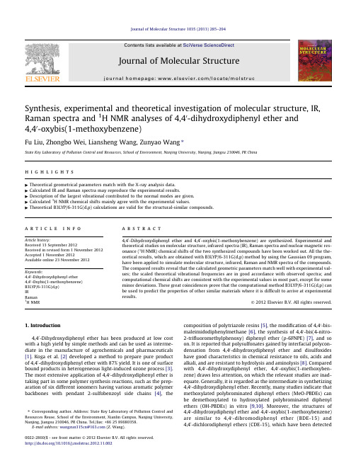
Synthesis,experimental and theoretical investigation of molecular structure,IR,Raman spectra and 1H NMR analyses of 4,40-dihydroxydiphenyl ether and 4,40-oxybis(1-methoxybenzene)Fu Liu,Zhongbo Wei,Liansheng Wang,Zunyao Wang ⇑State Key Laboratory of Pollution Control and Resources,School of Environment,Nanjing University,Nanjing,Jiangsu 210046,PR Chinah i g h l i g h t s"Theoretical geometrical parameters match with the X-ray analysis data."Calculated IR and Raman spectra may reproduce the experimental results."Description of the largest vibrational contributed to the normal modes are given."Calculated 1H NMR chemical shifts mainly agree with the experimental values."Theoretical B3LYP/6-311G(d,p)calculations are valid for the structural-similar compounds.a r t i c l e i n f o Article history:Received 13September 2012Received in revised form 1November 2012Accepted 1November 2012Available online 23November 2012Keywords:4,40-Dihydroxydiphenyl ether 4,40-Oxybis(1-methoxybenzene)B3LYP/6-311G(d,p)IRRaman 1H NMRa b s t r a c t4,40-Dihydroxydiphenyl ether and 4,40-oxybis(1-methoxybenzene)are synthesized.Experimental and theoretical studies on molecular structure,infrared spectra (IR),Raman spectra and nuclear magnetic res-onance (1H NMR)chemical shifts of the two synthesized compounds have been worked out.All the the-oretical results,which are obtained with B3LYP/6-311G(d,p)method by using the Gaussian 09program,have been applied to simulate molecular structure,infrared,Raman and NMR spectra of the compounds.The compared results reveal that the calculated geometric parameters match well with experimental val-ues;the scaled theoretical vibrational frequencies are in good accordance with observed spectra;and computational chemical shifts are consistent with the experimental values in most part,except for some minor deviations.These great coincidences prove that the computational method B3LYP/6-311G(d,p)can be used to predict the properties of other similar materials where it is difficult to arrive at experimental results.Ó2012Elsevier B.V.All rights reserved.1.Introduction4,40-Dihydroxydiphenyl ether has been produced at low cost with a high yield by simple methods and can be used as interme-diate in the manufacture of agrochemicals and pharmaceuticals [1].Koga et al.[2]developed a method to prepare pure product of 4,40-dihydroxydiphenyl ether with 87%yield.It is one of surface bound products in heterogeneous light-induced ozone process [3].The most extensive application of 4,40-dihydroxydiphenyl ether is taking part in some polymer synthesis reactions,such as the prep-aration of six different ionomers having various aromatic polymer backbones with pendant 2-sulfobenzoyl side chains [4],thecomposition of polytriazole resins [5],the modification of 4,40-bis-maleimidodiphenylmethane [6],the synthesis of 4,40-bis(4-nitro-2-trifluoromethylphenoxy)diphenyl ether (p -6FNPE)[7],and so on.It is reported that polysulfonates gained by interfacial polycon-densation from 4,40-dihydroxydiphenyl ether and disulfoxides have good characteristics in chemical resistance to oils,acids and alkali,and are resistant to hydrolysis and aminolysis [8].Compared with 4,40-dihydroxydiphenyl ether,4,40-oxybis(1-methoxyben-zene)draws less attention,on which the relevant studies are inad-equate.Generally,it is regarded as the intermediate in synthetizing 4,40-dihydroxydiphenyl ether.Recently,many studies indicate that methoxylated polybrominated diphenyl ethers (MeO-PBDEs)can be demethoxylated to hydroxylated polybrominated diphenyl ethers (OH-PBDEs)in vitro [9,10].Moreover,the structures of 4,40-dihydroxydiphenyl ether and 4,40-oxybis(1-methoxybenzene)are similar to 4,40-dibromodiphenyl ether (BDE-15)and 4,40-dichlorodiphenyl ethers (CDE-15),which have been detected0022-2860/$-see front matter Ó2012Elsevier B.V.All rights reserved./10.1016/j.molstruc.2012.11.002⇑Corresponding author.Address:State Key Laboratory of Pollution Control and Resources Reuse,School of the Environment,Xianlin Campus,Nanjing University,Nanjing,Jiangsu 210046,PR China.Tel./fax:+862589680358.E-mail address:wangzun315cn@ (Z.Wang).extensively in environment.The extensive application and the typ-ical structure of 4,40-dihydroxydiphenyl ether urge us to explore its environmental behavior and potential environmental risk.Vibrational spectroscopy and nuclear magnetic resonance (NMR)techniques are widely used in the research of molecular systems.Study on vibrational spectroscopy of compounds may provide a convenient way to understand molecular properties of theirs analogues and the degradation nature involving bond cleavage [11].Arguably NMR is one of the most sensitive and versatile analytical probes of molecular structure and dynamics of complex organic compounds [12].Hence,experimental and theoretical studies on the vibrational spectra and NMR chemical shifts would be of significance for understanding their environ-mental behavior and assessing their potential environmental risk [13].Furthermore,the density functional theory (DFT)method has been one of the most frequently used calculated methods in exploring molecular vibrational spectra in computational physics,chemistry,and material science [14–16].Some studies have revealed that the DFT computations,combining the hybrid exchange–correlation functional Becke-3–Lee–Yang–Parr (B3LYP)with the standard 6-311G(d,p)basis set,yield good and consistent results in molecular analyses [17–20].The combination of DFT calculations of chemical shifts and harmonic vibrational frequen-cies with experimental NMR and IR parameters has become an accepted technique to gather insight into the molecular structures [21].Thus,in the present study,we give experimental and computa-tional descriptions and characteristics of 4,40-oxybis(1-methoxy-benzene)and 4,40-dihydroxydiphenyl ether on geometrical parameters,vibrational properties and hydrogen chemical shifts.The structural parameters,vibrational frequencies and chemical shifts are calculated using the DFT/B3LYP method with the 6-311G(d,p)basis set.The aim is to check whether the B3LYP/6-311G(d,p)method is reliable to forecast the characteristics of other structural-similar compounds by comparing the agreement be-tween experimental and calculated results.2.Synthesis and experimental methodsThe two researched compounds were synthesized by ourselves.The general synthetic route is shown in Fig.1.2.1.Materials4-Methoxyphenol (AR),cuprous iodide (CuI,AR),and tetra-methylethylenediamine (TEMED,>98.0%)were purchased from Sinopharm Group Co.Ltd.4-Iodoanisole (99.5%)and cesium car-bonate (Cs 2CO 3,99.9%)were bought from Energy Chemistry Sa En Group.N ,N -dimethylformamide (DMF,99.5%)and hydrobromic acid (HBr,48%)were supplied by Aladdin Chemistry Co.Ltd.2.2.Synthetic steps(1)5mmol of 4-methoxyphenol and 5mmol of 4-iodoanisolewere dissolved in 15mL of DMF.Then,0.5mmol of TEMED (serves as ligand),12mmol of Cs 2CO 3(serves as base),together with 0.5mmol of CuI (as catalyst)were added intothe mixture.And the solution was heated to 150°C for 12h under nitrogen.After cooling to room temperature,the reac-tion solution was diluted with 50mL of water and extracted four times with 20mL of ethyl acetate.The extracted liquid was absterged with saturated sodium chloride solution and dried with anhydrous magnesium sulfate,and then filtered and concentrated.The obtained crude product was further eluted and purified by silica gel column chromatography (300–400mesh)with petroleum ether and ethyl acetate at the ratio of 30:1–15:1.Thus,we got 4,40-oxybis(1-methoxy-benzene)product and the purity was 95%.Then,the product was recrystallized from n -hexane for spectroscopic studies.1H NMR (CDCl 3,400MHz)d : 3.81(s,6H), 6.86(d,J =7.2Hz,4H),6.93(d,J =7.2Hz,4H);IR (KBr )t :3062,2956,1608,1509,1467,1455,1441,1298,1248,1104,835,762cm À1;Raman (Ar +)t :3066,3009,2953,2903,1604,1452,1242,1164,1029,872,837cm À1.(2)1mmol of 4,40-oxybis(1-methoxybenzene)which was syn-thesized according to the above method,mixed with 48%HBr,and the solution was heated to reflux for 16h at 160°C.After cooling to room temperature,the reaction liquid was evaporated to nearly dry in the rotary evaporator and then extracted with dichloromethane.The obtained crude product was further eluted and purified by silica gel column chromatography (300–400mesh)with petroleum ether and ethyl acetate at the ratio of 15:1–10:1.Hence,we gained the solid product,4,40-dihydroxydiphenyl ether,with 99%purity level.1H NMR (CDCl 3,400MHz)d :6.70(d,J =7.2Hz,4H), 6.75(d,J =7.2Hz,4H),9.17(s,2H);IR (KBr )t :3602,3035,1601,1502,1463,1285,1211,1157,844,828cm À1;Raman (Ar +)t :3066,1604,1247,1221,1190,1151,850,819,632cm À1.Finally,the target products of high purity can be used for the determination of molecular structure and spectral properties.2.3.ExperimentsThe crystals of 4,40-dihydroxydiphenyl ether suitable for X-ray analyses were grown from chloroform.A crystal was put on a glass fiber.The X-ray diffraction measurements were carried on a Non-ius CAD 4single-crystal diffractometer equipped with a graphite-monochromated Mo K a radiation (k =0.71073Å)by using an x /2h scan mode at 293K.The structure was solved by the direct method and refined by the full-matrix least squares procedure on F 2using SHELXL-97program [22].The FT-IR spectra of the title compounds diluted in the KBr pellets were measured on a Nicolet Nexus 870spectrophotometer in the range of 400–4000cm À1at room temperature.The Raman spectra were recorded on Renishaw Invia Raman microscope spectrophotometer in the 100–4000cm À1region.The excitation line at 514nm was emitted by an Ar +laser.The 1H NMR measurements of 4,40-dihydroxydiphenyl ether and 4,40-oxybis(1-methoxybenzene)were carried out using a Bruker DPX-300NMR spectrometer at room temperature with tetrameth-ylsilane (TMS)as an internal standard in dimethylsulfoxide-d 6(DMSO-d 6)and deuterochloroform (CDCl 3)respectively.286 F.Liu et al./Journal of Molecular Structure 1035(2013)285–294putational detailsGaussian09software[23]was used in the calculations of geo-metrical parameters,vibrational frequencies and chemical shifts. Qiu et al.[24]reported that DFT/B3LYP method was better than Hartree–Fock(HF)method in the calculation on structural geometrythe excitation wavenumber v0is19455.3cmÀ1,which corresponds to the wavelength of514nm of a Ar+laser),v i is the vibrational wavenumber of the i th normal mode(cmÀ1);while S i is the Raman scattering activity of the normal mode v i;f(a constant equal to 10À12)is a suitably chosen common normalization factor for all peak intensities;h,k,c and T are Planck and Boltzmann constants, speed of light and temperature in Kelvin,respectively.Table1Optimized parameters of4,40-oxybis(1-methoxybenzene)and4,40-dihydroxydiphenyl ether.Geometrical parameters B3LYP/6-311G(d,p)Exp.a4,40-Oxybis(1-methoxybenzene)4,40-Dihydroxydiphenyl ether Bond length(Å)c C1–C2 1.397 1.395 1.386(4)c C2–C3 1.401 1.397 1.359(4)c C3–C4 1.388 1.391 1.383(4)c C4–C5 1.397 1.395 1.384(4)c C5–C6 1.389 1.391 1.380(4)c C1–C6 1.397 1.393 1.380(4)c C5–O7 1.395 1.395 1.395(4)c C2–O14 1.373 1.378 1.382(4)c O14–H240.966c C16–H26 1.093c C16–H27 1.094c C16–H28 1.088c C16–O14 1.430Selected bond angle(°)A C1–C2–C3119.569119.858120.5(3)A C2–C3–C4120.583120.182120.9(3)A C3–C4–C5119.611119.751119.0(3)A C4–C5–C6120.160120.256120.0(3)A C5–C6–C1120.359119.998120.5(3)A C6–C1–C2119.715119.951119.0(3)A C4–C5–O7122.221122.396123.2(3)A C6–C5–O7117.502117.223116.7(3)Fig.2.The molecular structure and atom numbering of4,40-oxybis(1-methoxy-benzene)(top)and4,40-dihydroxydiphenyl ether(bottom).F.Liu et al./Journal of Molecular Structure1035(2013)285–2942874.Results and discussion4.1.Optimized structuresThe optimized structural parameters of the two compounds, which are calculated at the B3LYP/6-311G(d,p)level,are summa-rized in Table1,and shown in Fig.2,using a consistent atom numbering scheme.The experimental X-ray diffraction values of 4,40-dihydroxydiphenyl ether are also listed in Table1for comparisons.As shown in Table1,most of the calculated bond lengths and bond angles are slightly larger than the corresponding experimen-tal values.Differences between the calculated results and experi-mental data are reasonable based on a fact that the theoretical results are based on the gas phase,while the experimental data are obtained in the solid phase.The ranges of C–C bond lengths of4,40-dihydroxydiphenyl ether and4,40-oxybis(1-methoxyben-zene)are1.388–1.401Åand1.391–1.397Årespectively.The ether288 F.Liu et al./Journal of Molecular Structure1035(2013)285–294F.Liu et al./Journal of Molecular Structure1035(2013)285–294289Table2Comparison of the observed and calculated vibrational spectra of4,40-oxybis(1-methoxybenzene).Mode Exp.a Freq.Inte.(IR)Acti.(Raman)Assignments,PED c(>10%) IR Raman Unscaled Scaled b132093074 3.1573.8t C–H(79.6),b ring(10.1)23076w3208307312.1151.4t C–H(79.9),b ring(10.1)33066vs32003066 2.0163.5t C–H(82.4)43062w31993065 4.7512.5t C–H(82.7)531903056 2.5347.8t C–H(79)631893055 5.6253.5t C–H(82.3)731853055 4.8145.0t C–H(83.3)83185305519.7103.6t C–H(77.7)93009m3131299918.5174.2t asCH3(91.1)102956m2953m3131299935.7252.7t asCH3(91.8)112913m3053292546.6148.4t asCH3(98.9)123052292443.8175.1t asCH3(98.8)132903s299729017.8614.8t sCH3(91.4)142838m29962900123.027.9t sCH3(91.2)151608w1604m16621609 1.1351.5t ring(53.7),q C–H(34.8)161575w16531600 2.691.3t ring(52),q C–H(37.2)1716291577 3.9114.6t ring(62.8),q C–H(29.0)181509vs1619156814.915.2t ring(63.2),q C–H(26.7)191543149443.4 6.8q C–H(49.4),x CH3(12.2),b ring(28.8)201466m153********.8 1.9q C–H(45.3),x CH3(13.8),b ring(25.6)211452s150714577.425.1r CH3(81.9)221441m150********.515.4r CH3(74.8),q C–H(10.6)23149114437.740.9r CH3(96.1)24149014428.021.9r CH3(91.3)2514781430 6.69.8x CH3(63.9),q C–H(17.6)261419w1477140855.229.4x CH3(61.5),q C–H(21.2)27145414010.7 1.5q C–H(42.1),x CH3(12.6),b ring(34.9)281298m14471301 3.9 2.1t ring(33.8),q C–H(45.0)291295s134412870.215.6t ring(43.6),q C–H(17.0),x CH3(14.3),q C–O(17.1) 301329128272.2 4.3t ring(31.2),q C–H(23.4),x CH3(15.4),q C–O(19.9) 31132412780.0 5.3q C–H(65.5),q C–O(12.3)321248vs13201249 2.3 4.3t ring(11.7),q C–H(57.5),q C–O(21.8)331242m129012340.625.4t asC–O(29.1),t ring(32.2),q C–H(21.0),x CH3(12.9) 341195s1275120328.5130.6t asC–O(20.7),t ring(28.9),q C–H(22.0),x CH3(22.1) 351180s124311801111.1 1.9t asC–O(26.7),t ring(24.3),q C–H(26.1),x CH3(17.6) 361164s121911677.474.8t sC–O(21.0),t ring(33.3),q C–H(31.4)371155m120511650.679.5q C–H(13.0),x CH3(62.5),b ring(13.9)381203114255.314.3q C–H(14.9),x CH3(60.4),b ring(13.8)3911801139 4.3 4.4b ring(20.1),q C–H(64.9)40117611340.49.1b ring(26.3),q C–H(60.0)41117111330.7 2.5q CH3(75.8),x C–O(12.6)421104s11701091 1.170.2q CH3(61.2),x CH3(15.1),x C–O(13.7)431127108915.6 1.6b ring(25.3),q C–H(60.0)441032vs1125103113.1 1.1b ring(25.8),q C–H(59.0)451029w10651030149.50.6t C–O(36.9),b ring(30.2),q C–H(16.2)461007m1064990 4.532.9t C–O(38.3),b ring(31.6),q C–H(15.1)471023990 4.60.1q C–H(33.6),s ring(54.6)4810229320.5 1.1q C–H(34.9),s ring(56.7)499639290.10.3x C–H(82.7),s ring(10.8)509599080.30.0x C-H(82.2),s ring(10.4)519389060.5 1.7x C–H(73.3),s ring(17.7)52878m872vs9368610.20.1x C–H(73.7),s ring(16.0)53834vs837vs88983239.322.5t as C–O(16.4),b ring(44.3),q C–H(30.1) 54814s815vs85981833.734.4c ring(17.2),x C–H(61.9),b C–O(13.0)5584580781.20.3c ring(22.8),x C–H(68.2)5683379011.5168.9b ring(25.7),x C–H(48.3),q C–O(15.0)57816787 2.80.4x C–H(88.2)58762s813752 1.9 3.4x C–H(90.5)5977772349.57.7b ring(30.8),q C–H(21.4),q C–O(33.1)60698w693w747693 1.414.6s ring(32.7),x C–H(38.8),q C–O(21.7)61716674 5.4 3.3s ring(35.8),x C–H(42.3),x C–O(17.7)626966329.2 3.0s ring(36.1),x C–H(28.8),q C–O(25.8)63627w653628 2.631.6b ring(49.7),q C–H(26.2),q C–O(18.5)646496280.311.6b ring(79.2),q C–H(27.2)65524s6495258.1 3.5c ring(24.9),x C–H(39.2),q C–O(30.1)6654250812.1 5.7c ring(28.8),x C–H(22.1),q C–O(32.3)67504m501w52550429.10.6c ring(52.8),x C–H(39.8)685214497.1 3.0c ring(22.1),x C–H(33.6),x C–O(31.8)69464445 2.4 1.1b ring(21.7),x C–H(21.6),x C–O(50.3)704604210.513.7s ring(17.0),x C–H(21.9),q C–O(43.0),x CH3(21.0) 714354170.0 3.6c ring(65.2),x C–H(28.4)72431379 1.20.1c ring(64.1),x C–H(25.2)73391349 3.77.6c ring(19.4),x C–O60.1,q CH3(11.8)(continued on next page)bonds C5–O7,C2–O14and C16–O14are1.395Å,1.373Åand1.430Å. The range of C–H bond lengths of methyl is1.088–1.094Å.For both compounds,the calculated values of the C–C–C angles in the aro-matic rings are around the typical hexagonal angle of120°.The cal-culated values of the dihedral angles of C4–C5–O7–C8(À44.777°/ 139.136°for4,40-oxybis(1-methoxybenzene),andÀ44.531°/ 144.593°for4,40-dihydroxydiphenyl ether),which are a critical geometry parameter for conformers in the ground state,are closer to the experiment results(À34.8(5)°/149.2(3)°).The phenomenon demonstrates the non-planar nature of the two aromatic rings in the two compounds,which is attributed to the steric interaction. The calculation can be supported by the stereochemic study of Kurt Mislow[30–32].Qu et al.[13]reported that the sum of two dihe-dral anglesðC01—S—C1—C6;C1—S—C01—C06Þfor four types of TCDPSs(2,20,3,30-TCDPS,2,20,3,40-TCDPS,2,20,3,50-TCDPS,and2,20,3,60-TCDPS)is about equal to±90°,indicating that the plane of the two benzene rings are almost vertical to each other.In the present work,the same conclusion is reached based on the calculated re-sults.Dihedral angle C4–C5–O7–C8and C5–O7–C8–C9of4,40-oxy-bis(1-methoxybenzene)isÀ44.777°andÀ44.708°separately, and the corresponding value for4,40-dihydroxydiphenyl ether is À44.531°andÀ42.891°.The sum of the two angles isÀ89.485°andÀ87.422°,close toÀ90°.However,the sum of the two exper-imental data isÀ108.1(10)°,deviated fromÀ90°.The existence of extended hydrogen bonding in4,40-dihydroxydiphenyl ether and the stacking interaction may explain such results.For the two dihedral angles,there are some slight deviations between the two compounds and DPS(À50.1°/À49.5°(Cal.)andÀ49.6°/À49.6°(Exp.))[33],confirming that the steric effect of the substi-tuted functional groups on the dihedral angles of C4–C5–O7–C8 and C5–O7–C8–C9.4.2.Vibrational assignmentsCalculated and experimental IR and Raman spectra of the two compounds are shown in Figs.3and4,respectively.It is easy to discover that the main absorption peaks of the calculated spectra are mainly in accordance with those of the experimental spectra, demonstrating that the calculated results are dependable.How-ever,as to4,40-dihydroxydiphenyl ether,there are some differ-ences between the simulated spectra and the observed one, because thefluorescence effect reduces the quality of the experi-mental Raman spectra.4,40-oxybis(1-methoxybenzene)has31 atoms and87normal vibrational modes and4,40-dihydroxydiphe-nyl ether has25atoms and69normal vibrational modes.Theoretical(unscaled and scaled)and experimental vibrational fre-quencies(cmÀ1),peak intensities(km molÀ1)and the correspond-ing assignments for the vibrational modes are gathered in Tables 2and3.The tables also give PED values and the description of the largest vibrational contributions to the normal modes.It is a fact that the DFT method systematically overestimates the vibrational wavenumbers because of the neglect of anharmonicity effects in the real system[34].So,we use generic frequency scale factors tofit the theoretical results with experimental ones.More-over,previous studies have revealed increasing frequency overesti-mation of DFT in the high frequency regions(>3000cmÀ1)[35].As a result,the frequencies larger than3000cmÀ1are scaled down by multiplying a factor of0.958[36],while other frequencies are scaled down by a factor of0.9682[13,37].In addition,we use linear regression method to analyze the consistency between calculated and experimental frequencies.The results are given in Table4.The squared correlation coefficients R2are all greater than 0.99,showing that good linearity exist between theoretical fre-quencies and experimental values for the two compounds.In other words,the calculated results with Gaussian package can be used to predict vibrational frequencies.4.2.1.Ring vibrationsThe C–H and C–C related vibrations can help to determine the existence of aromatic rings in a structure.The C–H stretching vibrations of aromatic structures often occur in the range of 3000–3100cmÀ1.The nature of substituents has little influence on the band in this region[38,39].The C–H in-plane bending vibra-tions often appear in the region1000–1300cmÀ1.And750–1000cmÀ1is the C–H out-of-plane bending vibrational region.It is reported that the bands of the phenyl C–C stretching vibrations generally appear at1450cmÀ1,1500cmÀ1,1580cmÀ1,and 1600cmÀ1in IR spectra with variable intensities[40].For4,40-oxybis(1-methoxybenzene),the aromatic C–H stretch-ing vibrations appear at3076and3062cmÀ1in the IR spectrum with weak peaks,while with very strong intensity at3066cmÀ1 in Raman spectrum.Scaled theoretical C–H stretching modes are found to be at3073and3065cmÀ1.In IR spectrum,the frequencies 1298,1248and1032cmÀ1are assigned to the C–H in-plane bend-ing vibrations,and two intensive bands at814cmÀ1and762cmÀ1 are expected to be the C–H out-of-plane bending vibrations.The wavenumbers at698cmÀ1in IR and501cmÀ1in Raman spectra are ascribed to the C–H out-of-plane deformation.As shown in Table2,the IR wavenumbers1466cmÀ1,1509cmÀ1,1575cmÀ1 and1608cmÀ1,in agreement with the calculated data,areTable2(continued)Mode Exp.a Freq.Inte.(IR)Acti.(Raman)Assignments,PED c(>10%) IR Raman Unscaled Scaled b74360328 2.115.7c ring(12.3),x C–H(10.0),x C–O(51.9),q CH3(18.2) 75339314 1.5 1.4c ring(14.9),x C–H(10.0),x C–O(48.9),q CH3(19.2) 763243000.1 2.3b ring(21.4),x C–H(14.8),q C–O(42.9),x CH3(15.1) 77248240 2.3 1.1q CH3(53.1),q C–O(27.8)782452370.1 4.0c ring(16.8),x C–H(10.4),q CH3(62.9) 79227220 3.80.9q CH3(34.0),q C–O(41.7)801961900.6 4.8b ring(35.1),q C–O(57.3)81160155 1.8 2.7c ring(34.9),x C–O(33.3),x C–H(26.4) 82147142 3.10.4x ring(28.6),s C–O(66.2)838683 1.30.6x CH3(34.0),s C–O(52.8)847976 4.20.4x CH3(25.2),x ring(10.0),s C–O(59.9) 8556540.034.4b C–O(60.0),b CH3(10.7),x ring(20.4) 863130 1.210.4b C–O(81.1)8777 1.2 5.8b C–O(88.4)a vs,Very strong;s,strong;w,weak;m,medium.b With the scale factor of0.958for calculated wave numbers greater than3000cmÀ1and the scale factor of0.9682for other lower wavenumbers.c t,Stretching;t s,sym.stretching;t as,asym.stretching;b,in-plane-bending;c,out-of-plane bending;s,torsion;q,wagging;x,rocking;r,scissoring.290 F.Liu et al./Journal of Molecular Structure1035(2013)285–294F.Liu et al./Journal of Molecular Structure1035(2013)285–294291Table3Comparison of the observed and calculated vibrational spectra of4,40-dihydroxydiphenyl ether.Mode Exp.a Freq.Inte.(IR)Acti.(Raman)Assignments,PED c(>10%) IR Raman Unscaled Scaled b137813622139.8267.2t O–H(91.4)23602s37793620152.3249.6t O–H(91.4)332083074 4.7367.4t C–H(75.4)43066vs32063071 4.6453.2t C–H(75.6)53202306710.0309.9t C–H(59.0)6320130667.7355.4t C–H(59.1)73035w3191305714.9191.0t C–H(74.5)83191305715.7168.6t C–H(74.4)93179304617.0248.9t C–H(64.3)103179304519.2232.2t C–H(64.2)111873w1604m165916070.0185.4t ring(53.6),b C–H(39.3)121601w165115980.570.6t ring(54.7),b C–H(37.6)131594m164315918.1151.4t ring(54.1),b C–H(29.4),b COH(12.8)141637158513.129.5t ring(30),b C–H(41.6),b COH(14.6)151502vs15401491101.3 4.8t ring(54.6),b C–H(55.2)161463vs152********.3 1.3t ring(34.8),b C–H(55.4)171479143255.80.5t ring(35.2),b C–H(41.6),b COH(14)181383s14701423117.40.1t ring(31.6),b C–H(43.2),b COH(13.8)191362m1384134082.4 6.0t ring(38),b C–H(37.6),b COH(17.1)2013801336115.57.5t ring(32.4),b C–H(44.4),b COH(18.6)211285w13321290 1.8 2.1t ring(23.8),q C–H(56.6),b C–O(11.4)22131412728.4 1.5t ring(26.6),q C–H(51.6),b C–O(12.2)231249s1247m12891248233.935.6t asC–O(17.6),t ring(31.2),q C–H(24.6),b COH(17.3) 241221w12641224 2.059.6t ring(40.4),q C–H(35.4),t COH(16.3)251211vs12541214252.7 3.8t asC–O(21.6),t ring(25.4),q C–H(35.4)261190w1224118554.365.5t sC–O(18.5),t ring(33.3),b C–H(33.0)271151s12061167280.7142.8b COH(30.8),t ring(26.2),b C–H(30.2)281157s12021163838.119.2b COH(31.0),t ring(29.2),b C–H(28.0)2911801142 6.011.1b C–H(73.4),t ring(12.8)301142m11781140 3.230.6b C–H(66.4),t ring(16.6)311123108729.2 1.1b C–H(60.7),b ring(26.3)321097vs1120108544.9 1.1b C–H(59.6),b ring(24.8)331009m102799410.6 1.5t ring(55.6),b C–H(34.0)34102599310.2 1.1t ring(84.2),b C–H(34.4)359579270.20.2x C–H(83.1),c ring(11.1)369499190.40.1x C–H(82.8),c ring(10.8)37940910 2.3 1.1x C–H(73.0),c ring(17.2)38932903 1.00.6x C–H(75.3),c ring(17.4)39874w89286430.225.7t asC–O(13.8),b ring(49.9),b C–H(34.6)40844m850s86083345.976.8c C–H(53.6),t asC–O(18.5),t COH(17.7),b ring(25.0) 41819s84481794.897.4c C–H(59.1),b C–O(17.9),t COH(21.0),b ring(14.5) 42828vs841814126.941.1x C–H(78.2),c ring(20.9)43816790 3.8 2.0x C–H(85.8)44811785 2.9 2.3c C–H(47.4),t COH(15.7),b C–O(10.7),b ring(18.5) 45791s798773165.7 6.5x C–H(80.3)46755731 6.17.1s ring(32.2),x C–H(37.1),b C–O(17.7)47716693 5.0 2.0s ring(38.6),x C–H(32.8),b C–O(11.0)4870668314.7 4.9s ring(37.4),x C–H(33.7),c COH(10.6),t sC–O(12.4) 49654633 4.613.7b ring(53),b C–H(28.2)50632w652631 1.625.7b ring(47.9),b C–H(24.3)51587m584w58957015.28.2c C–H(41.5),b C–O(17.9),b ring(36.7)52507m52350751.70.4c ring(31.8),c C–H(47.3),c COH(14.8)53492w50849213.8 6.5b ring(65.2),x C–H(28.3)54490m50548917.0 3.7x C–H(41.8),c ring(34.4),c COH(17.0)55451437 3.5 3.5c C–O(38.7),b COH(20.6)564324180.4 2.1s ring(40),x C–H(23.2)57429415 1.00.2s ring(39.6),x C–H(24.2)584254117.0 4.3c COH(33.2),x C–O(19.9)59408395213.8 2.5s C–O(29.8),c COH(28.4)60396383222.3 3.6s C–O(25.8),c COH(35.4)6137736539.0 5.6c COH(69.2)62357w349338 3.815.3c COH(76.6)6331630611.2 1.4c C–O(28.6),c COH(38.0)64278w272264 1.38.2b ring(29.4),s COC(31.9)651651600.3 1.0c ring(21.6),c COH(27.8),b C–O(18.2)661451400.90.4c C–O(37.9),c COH(35.2),c ring(37.6)6763610.124.1s C–O(42.5)684746 1.927.6s C–O(77.5)692120 2.29.2s C–O(88.4)a vs,Very strong;s,strong;w,weak;m,medium.b With the scale factor of0.958for calculated wave numbers greater than3000cmÀ1and the scale factor of0.9682for other lower wavenumbers.c t,Stretching;t s,sym.stretching;t as,asym.stretching;b,in-plane-bending;c,out-of-plane bending;s,torsion;q,wagging;x,rocking.assigned as the aromatic C–C semicircle stretching vibrations.The aromatic ring C–C stretching vibration in observed Raman spec-trum is found at1604cmÀ1.As shown in Table2,the predicted vibrations assigned to phenyl ring vibrations are in good accor-dance with the experimental assignments.For4,40-dihydroxydiphenyl ether,the weak band observed at 3035cmÀ1in IR spectrum and the strong band at3066cmÀ1in Ra-man spectrum are assigned as the aromatic C–H stretching vibra-tion.In IR spectrum,the C–H in-plane bending vibrations are observed at1211cmÀ1and1097cmÀ1,and two intensive bands at844cmÀ1and828cmÀ1are expected to be the C–H out-of-plane bending vibrations.The wavenumbers at791cmÀ1in IR and 492cmÀ1in Raman spectra are ascribed to the C–H out-of-plane deformation.1463cmÀ1,1502cmÀ1and1601cmÀ1in IR spectrum are assigned as the aromatic C–C semicircle stretching vibrations, in agreement with the calculated data shown in Table3. 1604cmÀ1and1594cmÀ1are assigned as the aromatic ring C–C stretching vibration in observed Raman parisons demonstrate that all the experimental values match with the the-oretical frequencies.The wavenumbers appearing at1000cmÀ1are usually assigned as the trigonal ring breathing vibrations[41].For4,40-dihydroxydi-phenyl ether,the band at1009cmÀ1,which coincides with the calculated value994cmÀ1,is assigned to this mode.And for 4,40-oxybis(1-methoxybenzene),the experimental and calculated value is1007cmÀ1and990cmÀ1,respectively.The overtone of aromatic ring is observed at1875cmÀ1in the IR spectrum of 4,40-oxybis(1-methoxybenzene),and for4,40-dihydroxydiphenyl ether,the band is at1873cmÀ1.However,there is no correspond-ing peak in the theoretical spectra.The medium peaks at874cmÀ1 for4,40-dihydroxydiphenyl ether and834cmÀ1for4,40-oxybis (1-methoxybenzene)in experimental IR spectra are the contribu-tion of the coupling of the skeleton vibration of the aromatic ring and the C–O asymmetric stretching.4.2.2.C–O vibrationsThe frequencies around1270–1230cmÀ1in IR spectrum are re-garded as the C–O stretching band of the aromatic ether. 1249cmÀ1is assigned to C–O asymmetric stretching vibrations for4,40-dihydroxydiphenyl ether and1195cmÀ1and1180cmÀ1 for4,40-oxybis(1-methoxybenzene).The small differences may be explained by the different functional groups in the para-position. And the associated dominated vibration mode is the coupling of C–O asymmetric stretching and C–H in-plane bending vibrations. Moreover,in the experimental Raman spectrum,the C–O asymmetric stretching vibration appears at1247cmÀ1,and the symmetric stretching vibration wavenumber is1190cmÀ1for 4,40-dihydroxydiphenyl ether.For,1242cmÀ1is assigned to the asymmetric stretching vibration,and the symmetric stretching vibration is found at1164cmÀ1.C–O in-plane bending vibrations are observed at850cmÀ1for4,40-dihydroxydiphenyl ether,and at837cmÀ1and693cmÀ1for4,40-oxybis(1-methoxybenzene). The experimental values match well with the theoretical data in Tables2and3.4.2.3.O–H and–CH3vibrationsFor un-substituted phenol,the frequency of O–H stretching vibration in the gas phase is3657cmÀ1[42].Sundaraganesan et al.[43]assigned a strong band in FT-IR spectrum at3387cmÀ1 and a weak band in FT-Raman at3390cmÀ1to O–H stretching vibration in5-amino-O-cresol.In the present work,the strong band observed at3602cmÀ1is assigned to O–H stretching mode, and the calculated O–H band is at3619cmÀ1.There is a small devi-ation between the calculated and the experimental data.Although the band is not observed in the experimental Raman spectrum,it is calculated to be3621cmÀ1.In addition,phenols have the in-plane bending vibrations in the band region1152–1250cmÀ1[37].The weak band observed at1285cmÀ1and the strong band observed at1157cmÀ1in IR spectrum are assigned as O–H in-plane bending vibrations.The theoretically computed values at1272and 1167cmÀ1havefine consistency with the experimental results. The O–H out-of-plane bending vibrations for phenol lie in the 290–320cmÀ1region for free O–H[41].In the present work,the scaled values of O–H out-of-plane deformation vibration are calcu-lated to be338cmÀ1and365cmÀ1,and the corresponding Raman experimental value is357cmÀ1,but not observed in the IR spectra.The CH3asymmetric stretching modes are found in the region of 2956–2913cmÀ1in IR and3099–2953cmÀ1in Raman spectrum. The symmetric stretching vibration of CH3is found at2838cmÀ1 in IR and2903cmÀ1in Raman spectrum.Peaks at1441cmÀ1in IR and1452cmÀ1in Raman spectra,in accordance with predicted frequencies at1444and1457cmÀ1,are assigned to the scissoring of CH3.The wagging vibrations are found at1104and1155cmÀ1in IR spectrum,with the predicted frequencies at1091and 1165cmÀ1.In this range,the wagging vibrations of methyl group mostly occur with aromatic ring vibrations.4.3.1H NMR chemical shiftsNMR is the most powerful method in analytical chemistry for the identifications of structural groups and reactive ionic species.Table4Correlation analysis of calculated and experimental vibrational frequencies.Molecule Correlation equations R24,40-Oxybis(1-methoxybenzene)IR:k Exp.=0.9897k Cal.+15.8240.9995Raman:k Exp.=0.9983k Cal.+2.11410.99994,40-Dihydroxydiphenyl ether IR:k Exp.=0.9955k Cal.À0.46770.9982Raman:k Exp.=0.9922k Cal.+10.6330.9998Table5Comparison of theoretical and experimental values of1H NMR chemical shifts.Molecule d HCalc.(ppm)Exp.(ppm)Assignments 4,40-Oxybis(1-methoxybenzene)7.137 6.945H-21(H-25)6.861 6.927H-19(H-22)6.700 6.874H-20(H-20)6.491 6.856H-18(H-24)3.449 3.805H-26(H-27,H-28,H-29,H-30,H-31)4,40-Dihydroxydiphenyl ether7.010 6.771H-19(H-23)6.780 6.753H-17(H-21)6.670 6.718H-18(H-20)6.397 6.700H-16(H-22)3.2829.168H-24(H-25)292 F.Liu et al./Journal of Molecular Structure1035(2013)285–294。

反量化英语Quantification has become an increasingly prevalent aspect of modern life, with data and metrics being used to measure and evaluate various facets of our existence. While this trend has brought about numerous benefits, it has also given rise to a growing concern regarding the potential drawbacks of an over-reliance on quantification. In this essay, we will explore the concept of "anti-quantification" and examine the arguments for a more balanced approach to the role of data and metrics in our lives.One of the primary arguments against the excessive use of quantification is the inherent reductionism inherent in the process. By reducing complex phenomena to numerical values, we risk oversimplifying the nuances and contextual factors that contribute to the richness and depth of human experience. This can lead to a distorted understanding of reality, where the quantifiable aspects are prioritized at the expense of the qualitative and intangible elements that are equally, if not more, important.Moreover, the reliance on quantification can foster a culture of obsession with metrics and a fixation on numerical targets, often at the expense of deeper, more meaningful goals. This can manifest invarious domains, from education, where test scores become the primary measure of success, to healthcare, where patient outcomes are reduced to a series of statistics. In such scenarios, the true purpose of these institutions – to nurture well-rounded individuals and promote holistic well-being – can become obscured.Another concern with the overuse of quantification is the potential for unintended consequences and the distortion of behavior. When individuals and organizations are evaluated primarily based on numerical targets, they may be tempted to manipulate or game the system in order to achieve those targets, even if it means sacrificing integrity or ethical considerations. This can lead to a culture of mistrust, where the reliability and validity of the data become increasingly questionable.Furthermore, the reliance on quantification can contribute to a sense of dehumanization, where individuals are reduced to mere data points, stripped of their unique experiences, emotions, and personal narratives. This can have profound implications for our social interactions, decision-making processes, and the way we perceive and value one another.In response to these concerns, the concept of "anti-quantification" advocates for a more balanced and nuanced approach to the use of data and metrics. This perspective recognizes the value ofquantification in certain contexts, such as scientific research, policy-making, and decision-support systems, but also acknowledges the need to temper its application with a deeper understanding of the qualitative and contextual factors that shape human experiences and societal dynamics.At the heart of the anti-quantification movement is a call for a greater emphasis on the subjective, the experiential, and the intangible aspects of life. This includes a focus on narrative, storytelling, and the exploration of the human condition through the arts, humanities, and social sciences. By embracing these alternative modes of understanding, we can cultivate a richer, more nuanced perspective on the world around us, one that acknowledges the inherent complexity and diversity of human experiences.Moreover, the anti-quantification approach encourages a more critical and reflective stance towards the use of data and metrics. This involves questioning the underlying assumptions, methodologies, and potential biases that shape the collection and interpretation of data, as well as a willingness to challenge the dominant narratives and preconceptions that often drive the quantification agenda.In practical terms, the implementation of anti-quantification principles could involve a range of strategies, such as the incorporation of qualitative assessments alongside quantitativemeasures, the emphasis on contextual factors in decision-making processes, and the fostering of interdisciplinary collaborations that bridge the divide between the quantitative and the qualitative.Ultimately, the call for anti-quantification is not a rejection of the value of data and metrics, but rather a recognition of the need to strike a balance between the quantifiable and the intangible, the objective and the subjective, in order to create a more holistic and meaningful understanding of the human experience. By embracing this approach, we can work towards a future where the richness and complexity of our lives are not reduced to mere numbers, but instead celebrated and understood in all their nuanced glory.。

Chapter3Persistent Scatterer InSARIn Chap.2,the physical mechanism of subsidence due to hydrocarbon production and deformation estimation methodologies have been discussed.This chapter intro-duces InSAR as a measurement technique for deformation monitoring.InSAR utilizes phase difference observations between two radar acquisitions for the estimation of surface deformation.Various SAR missions are currently oper-ational,such as ERS-2and Envisat,acquiring SAR images that cover an area of 100×100km with a35day time interval,at800km height,using C-band wave-length of56mm.Interferometric phase observations can be obtained with millime-ter precision.However,besides the deformation signal of interest,the interferomet-ric phase also contains contributions due to atmospheric signal delay,topography and orbital errors.Moreover,only the fractional phase is observed,which implies that the number of integer cycles from satellite to surface is unknown.Conventional InSAR can only be successfully applied in areas that do not suffer from significant surface changes in time,whereas the deformation signal has such magnitude that error sources are negligible.Subsidence due to hydrocarbon production in the Netherlands has a small mag-nitude(<1cm/year)and a large spatial extent(the extent of the Groningen gasfield is∼30km).Furthermore,the area of interest has an agricultural character and is subject to surface changes(temporal decorrelation).Hence,an accurate estimation of the error sources,such as atmospheric disturbances,is very important.Therefore, a time series of SAR acquisitions is utilized to detect reliable measurement targets, based on their reflectivity behavior through time:the so-called Persistent Scatterers (PS)(Ferretti et al.,2000).In this chapter,the estimation of deformation from PS phase observations is ex-plained(functional model,stochastic model,and estimation procedure).It starts with an overview of interferometric processing.Subsequently,the selection of Per-sistent Scatterer candidates is addressed in Sect.3.2.Several strategies have been developed to estimate deformation from the PS observations(Ferretti et al.,2001; Berardino et al.,2002;Kampes,2005).In this research,the Delft implementation of Persistent Scatterer InSAR(DePSI)has been applied.The mathematical framework underlying DePSI is explained in Sect.3.4.The functional and stochastic models for PSI are considered from a theoretical point of view in this chapter.The actual appli-cation of DePSI for subsidence monitoring in the Netherlands will be addressed in Chap.6.3.1Interferometric ProcessingSAR images consist of a grid of complex observations that can be addressed to sin-gle resolution cells.These complex observations stem from the superposition of all V.B.H.(Gini)Ketelaar,Satellite Radar Interferometry,27 Remote Sensing and Digital Image Processing14,©Springer Science+Business Media B.V.2009283Persistent Scatterer InSARFig.3.1Left:image geometry of a SAR acquisition(Hanssen,2001).The satellite velocity v s is approximately7km/s.The dark grey area indicates the footprint of a single pulse.The total coverage of a SAR scene,between early and late azimuth,and near and far range,is depicted in light grey.Right:repeat-pass InSAR and detection of deformation by means of phase difference observationsscattering targets within the resolution cell.The range resolution of a SAR acquisi-tion depends on the system’s bandwidth(Hanssen,2001).ERS-2for example has a range bandwidth of15.55Mhz,which corresponds with a range resolution of9.6m. In azimuth direction,the Doppler bandwidth is utilized for optimizing the azimuth resolution.The Doppler bandwidth of ERS-2is∼1378Hz.The Pulse Repetition Frequency(PRF)is a higher,1680Hz,to fully sample the Doppler spectrum.The pixel spacing of a SAR image is closely related to the resolution.The pixel spacing is determined by the sampling rate.For ERS-2,the range sampling rate is 18.96Mhz.The ERS-2pixel spacing in range direction is7.9m,which corresponds with∼20m in ground range.The ERS-2azimuth spacing is4m.In this book,the term pixel is used as the area covered by the pixel spacing,although strictly speaking a pixel is a infinitesimally small point that represents the resolution cell(Hanssen, 2001).Each object on earth is observed by consecutive pulses,appearing in different range bins in the raw data.By means of focusing,these observations are shifted to a common range bin.In this research,the input in the interferometric processing chain are the focused Single-Look Complex(SLC)images.Each complex observation can be converted into an amplitude and a phase ob-servation.The amplitude represents the strength of the reflection towards the sensor from the resolution cell.An interferogram is computed by the complex multiplica-tion of the observations in each resolution cell from two coregistered SAR images: a‘master’and a‘slave’image.The interferometric phase differences are the actual observations from which earth surface deformation is estimated.The computation of interferograms in this research has been performed by the Delft Object-oriented Radar Interferometric Software(Doris)(Kampes and Usai, 1999).The key steps are summarized in Fig.3.2.3.1Interferometric Processing29Fig.3.2Schematic overview of interferometric processing.A master(M)and a slave acquisi-tion(S)are oversampled and coregistered.The interferogram is computed from the complex mul-tiplication of the master image and the resampled slave image.In the last stage,the reference phase of the ellipsoid is subtracted3.1.1OversamplingAfter reading the SLC data and the precise orbits,the SAR images are oversampled with a factor2prior to the coregistration and the formation of interferograms.Over-sampling with a factor2is performed to avoid aliasing in the complex multiplication of the SAR images.Since the equivalent of a multiplication in the space domain is a convolution in the frequency domain,the spectrum length(both in azimuth and range)will be doubled after complex multiplication of two SAR images.The effect of oversampling is illustrated in Fig.3.3and Fig.3.4.For ERS,the pulse repeti-tion frequency is1680Hz,while the azimuth bandwidth is1378Hz.After over-sampling,the pulse repetition frequency is3360Hz,which avoids aliasing in the complex multiplication.In the determination of the minimal oversampling factor, the Doppler centroid frequency shift has to be compensated.The Doppler centroid frequency is the center frequency of the passage of a scatterer through the antenna beam.ESA’s SLC images are zero-Doppler processed,which means that the corre-sponding satellite position can be found by an orthogonal projection on the precise orbits.However,during the actual acquisition,the true Doppler centroid is never aimed exactly perpendicular to theflight direction.Therefore,the SAR data spec-trum is shifted in azimuth direction.An overview of this mechanism can be found303Persistent Scatterer InSARFig.3.3Original SAR image spectrum(left)and after oversampling with a factor of2(right)Fig.3.4SAR image spectrum after oversampling with a factor of2(left)and after complex multi-plication(right).The size of the spectrum is doubled after oversampling;due to the oversampling, aliasing does not occurin Hanssen(2001).For ERS-2acquisitions with high Doppler centroid frequencies (>2000Hz),oversampling with a factor2may not be sufficient to avoid aliasing. An oversampling factor of2avoids aliasing of Doppler shifts up to990Hz;a factor 4covers Doppler shifts up to2670Hz.Some ERS-2acquisitions exhibit even higher Doppler deviations,requiring even higher oversampling factors.The radar coordinates of an oversampled image are at sub-pixel level with re-spect to the original sampling rate.This implies that a target’s location in the radar coordinate system can be more precisely determined in an oversampled image. 3.1.2CoregistrationThe oversampled SLC images together with the precise orbits(Scharroo and Visser, 1998;Doornbos and Scharroo,2004)form the input for the coregistration of the master and the slave image.Coregistration is a crucial step.If its precision is not3.1Interferometric Processing31Fig.3.5Spatial distribution of observations for the estimation of the coregistration polynomial (left)and standard deviation of the coregistration residuals per acquisition(right).The coregistra-tion windows are evenly distributed over the area,also in rural parts.The part of the image that does not contain window locations is covered with water.The standard deviation of the coregistration residuals is∼0.1and∼0.2oversampled pixels in range and azimuth direction respectively.This is equivalent to∼0.05and∼0.1pixels in range and azimuth direction in the original resolutionsufficient,it deteriorates the PS selection process and decreases the PS phase obser-vation precision.In the northeastern part of the Netherlands,the height differences are small(<30meters).Here,coregistration can be performed by a second degree polynomial.For the estimation of an accurate coregistration polynomial,it is essen-tial that the coregistration windows are evenly distributed over the area of interest. Especially in rural areas that are affected by temporal decorrelation,a proper choice of coregistration windows is required.Hence,a large number of candidate windows have been placed around evenly distributed local amplitude maxima,which are as-sumed to correspond with terrain features that are stable in time.The coregistration polynomial is estimated from a set of corresponding locations in master and slave acquisitions that are acquired from correlation optimization be-tween the(oversampled)candidate windows.To remove outliers,a geodetic testing procedure is applied(Teunissen,2000b;Kampes,2005).In this step,it is important that the size of the test,which determines the likelihood of rejecting a good obser-vation(type I error),is not set too strict.If too many observations are incorrectly rejected,the spatial coverage of the observations decreases,which results in inaccu-rately extrapolated coregistration vectors in rural areas with few PS candidates.Figure3.5shows an example of the spatial distribution of the accepted observa-tions in the estimation of the coregistration polynomial.The locations with a high observation density correspond with the city areas.The areas that are covered with water do not contain any observations,due to temporal decorrelation.The standard deviation of the coregistration residuals is approximately0.1and0.2pixel in range and azimuth direction respectively(oversampling factor2).By depicting the spa-tial distribution of the coregistration observations and their residuals,images with inaccurate coregistration are easily detected.323Persistent Scatterer InSARFig.3.6Interferogram before(left)and after(right)subtraction of the reference phase.The tem-poral and perpendicular baseline are140days and166m respectively.The repetitive line pattern (left)depicts the phase contribution due to the ellipsoidal shape of the earth.After subtraction of the reference phase,only urban areas appear coherent in the interferogram(right).Large parts of the image are noisy due to temporal decorrelation.The SAR data has been provided by ESA 3.1.3Interferogram ComputationAfter the estimation of the coregistration polynomial,the slave image is resam-pled to the master image geometry.Subsequently,the interferogram is computed by complex multiplication of the master image and the resampled slave image ob-servations.In the last step,the interferometric phase contribution due to the ellip-soidal shape of the earth is subtracted.Figure3.6depicts the interferogram before and after reference phase subtraction.The repetitive fringe pattern in the interfero-gram before subtraction of the reference phase depicts the phase contribution due to the ellipsoidal shape of the earth.After subtraction of the reference phase,the urban areas that contain coherent man-made features and the rural areas that suf-fer from temporal decorrelation can be distinguished.The interferometric phase not only represents surface deformation,but contains contributions due to atmospheric disturbance,topographic height differences,and residual orbital errors as well.To estimate deformation in the presence of other phase contributions,a network of mea-surement points(the Persistent Scatterers)will be selected by using a time series of SAR acquisitions.The selection of these measurement points is addressed in the next section.3.2Persistent Scatterer SelectionNot all phase observations in an interferogram contain useful information.The earth surface covered by a resolution cell may change in time,targets may not reflect back in the satellite direction,or they may not have the physical properties to be observed with a high enough Signal-to-Noise Ratio(SNR).In order to select coherent,i.e. interpretable,measurement points,candidate targets are selected that have a strong and consistent reflection in time(the Persistent Scatterers(Ferretti et al.,2000)).3.2Persistent Scatterer Selection33 These targets can often be attributed to a single physical object(‘man-made fea-ture’)that acts as a dominant scatterer within the resolution cell.Many of them behave like point scatterers,and can be observed from a wide range of viewing angles.These point scatterer observations are therefore less sensitive for the effec-tive(perpendicular)baseline between the master and slave acquisition.A Persistent Scatterer does not necessarily have to be a dominant point scatterer within the reso-lution cell.Distributed scatterers,such as rocks,can act as PS as well,although with a different dependency on the viewing geometry,i.e.the perpendicular baselines.This section addresses the selection of PS candidates.It explains the methodolo-gies to select targets with a high likelihood of coherent phase behavior from a time series of SAR acquisitions.3.2.1Identification Methods of PS CandidatesIn order to estimate all interferometric phase contributions(surface deformation, topographic heights,atmospheric disturbances,etc.)and maintain an efficient al-gorithmic approach,afirst order network is constructed from the potentially most reliable PS candidates.Since the interferometric phase observations are wrapped and the phase contribution due to the unknown deformation is contaminated by sev-eral‘error sources’,the amplitude observations of the PS candidates are utilized. Existing methodologies can be subdivided into three groups that use the following parameterization to select PS candidates:1.Signal-to-Clutter Ratio(SCR)(SCR,1993),2.normalized amplitude dispersion(D a)(Ferretti et al.,2001),and3.supervised classification(Humme,2007).SCR estimation is based on the assumption that a PS observation consists of a de-terministic signal that is disturbed by random circular Gaussian distributed clutter, see Fig.3.7.The deterministic signal stems from the dominant scatterer within the resolution cell.The clutter reflects the distributed scatterers in the surroundings of the point scatterer.The relation between SCR and the phase variance is defined as(SCR,1993):SCR=s2c2;σ2ψ=12·SCR(rad),(3.1)whereσ2ψis the phase variance of a single SAR observation,s represents the ampli-tude of the dominant scatterer and c the clutter in the surroundings.A scatterer with a high SCR through time is labeled as a PS candidate.SCR assumes stationary stochastic behavior of the surroundings of the scatterer,which may not be valid,especially in urban areas that contain multiple scatterers at a short distance that are likely to interfere.Practical implementation of SCR estimation is therefore not straightforward.Automatic distinction of two nearby PS candidates requires highflexibility of SCR estimation windows and signal edge detectors.343Persistent Scatterer InSARFig.3.7Complex PS observation that consists of a deterministic signal with superposed Gaussian distributed clutter (solid arrow lines).The deterministic signal represents the dominant scatterer within the resolution cell.The small dashed arrow line indicates the resultant of the clutter signal,which imposes the uncertainty on the phase observation of the dominant scattererThe normalized amplitude dispersion method (Ferretti et al.,2001)performs an amplitude time series analysis,in stead of a spatial analysis.Each pixel is quantified by the ratio between the dispersion of the amplitude σa and the mean μa of the amplitudes through time:D a =σa μa.(3.2)Point scatterers with a low normalized amplitude dispersion have a low phase dis-persion.Hence,they are selected as PS candidates.A direct relation exists between the normalized amplitude dispersion D a and SCR (SCR,1993):D a =1√.(3.3)A typical threshold for the normalized amplitude dispersion is 0.25(Ferretti et al.,2001),which corresponds with a SCR of 8.PS candidate selection based on SCR and normalized amplitude dispersion are using the amplitude observations.Phase stability as a selection criterium for PS candidates has been investigated as well (Hooper et al.,2004).The phase stability is analyzed under the assumption that deformation is spatially correlated.The phase observations of neighboring PS candidates are averaged,and those with the lowest residual noise are selected.However,with the typical land use in the Netherlands (scattered cities and villages separated by agricultural and vegetated areas)only a small percentage of the pixels in an interferogram contains Persistent Scatterers.Hence,also for this method,a pre-selection is made based on the amplitude obser-vations.3.2Persistent Scatterer Selection35Recently,supervised classification to select PS candidates has been investigated as well(Humme,2007).In areas where the distribution of PS is crucial for the esti-mation of the signal of interest,the possibility of omitting a PS candidate is reduced by manual selection of pixels that contain the reflection of man-made features.For the selection of PS candidates,it is essential that the amplitude observations are not affected by satellite system characteristics and viewing geometry.To obtain the amplitude observations that represent solely the physical characteristics of the PS candidates,SAR amplitude calibration is performed.The next section introduces a new method that does not perform the amplitude calibration explicitly,and hence saves a considerable amount of computation time.3.2.2Pseudo-calibrationFor an unbiased selection of PS candidates based on amplitude,SAR calibra-tion is performed to isolate the amplitude observations corresponding with phys-ical PS properties from amplitude variations due to viewing geometry and sensor characteristics.A method to perform SAR calibration is the ESA ERS SAR cali-bration(Laur et al.,2002).This SAR calibration method quantifies the satellite sys-tem characteristics.The amplitude observations are corrected for the varying system characteristics by means of a multiplication factor.This multiplication factor is built up from constant factors per acquisition(calibration constant,antenna pattern gain, replica pulse power);factors that depend on viewing geometry(range,incidence angle)and a factor that varies over the entire image(power loss).The ESA SAR calibration method is useful for thematic interpretation purposes, where amplitude values have to be compared over the entire SAR image.The vari-ation of the location of a Persistent Scatterer within a time series of SAR images is nevertheless limited.For PS selection,there is no need to be able to compare am-plitude values between near and far range.It is sufficient to determine calibration factors that are valid in the near surroundings of the PS.Moreover,uncalibrated am-plitude observations of potential PS candidates themselves can be utilized for the estimation of the calibration factors,since they correspond with man-made features that are not affected by temporal decorrelation.This has resulted in the development of empirical calibration methods,that are sensor independent(Bovenga et al.,2002; Cassee,2004).The newly developed calibration method that is described in this section goes one step further:it does not perform empirical calibration explicitly but evaluates if the PS candidate would have been selected if calibration would have been per-formed.It is referred to as pseudo-calibration.This method has the advantage that it saves computation time and storage space for calibrated images,especially since the amount of PS is generally a small percentage of the full image(1–2%or lower)and only their interferometric phase observations are used for the estimation of the de-formation signal.In this section,the mathematical framework for pseudo-calibration is described and its application to real data.363Persistent Scatterer InSAR 3.2.2.1Mathematical ModelEmpirical SAR calibration is implemented as a Gauss-Markov model that consists of a functional and stochastic model.The observations are the amplitudes of poten-tial PS candidates;the unknowns are the amplitude multiplication factors per image (the calibration factors).Since the sensor characteristics and viewing geometry vary smoothly over a SAR image,the image is subdivided into patches where the amplitude multiplication fac-tors are assumed to be constant.In each of these patches,potential PS candidates are selected based on the normalized amplitude dispersion that is computed from the stack of uncalibrated images.For a selection of P neighboring potential PS can-didates,a multiplication factor c k is estimated with respect to a reference image for all K SAR acquisitions.The functional and stochastic model read:E{y}=E{a k p}=c k a ref p;D{y}=Pp=1σ2apQ p,(3.4)where a k p is the amplitude observation for PS candidate p in image k with its vari-anceσ2ap.The unknown amplitude for PS candidate p free from variations due to sensor characteristics and viewing geometry is represented by a ref p.As the calibra-tion factors can only be estimated relatively,one calibration factor isfixed at the value1.Solving the system of equations from(3.4)results in a set of calibration factors that are utilized for pseudo-calibration.The stochastic model from(3.4)is not very well known a-priori.It is assumed that the amplitude variance reflects the physical properties of the PS candidates superposed on random noise due to viewing geometry(incidence and squint angle). Its initial value is derived from the amplitude dispersion(amplitude variance)in the uncalibrated stack.Based on the adjustment residuals,variance factor(s)to update the stochastic model are estimated by variance component estimation(VCE)(Teunissen,1988), see Sect.2.3.1.In the SAR calibration validation either one variance factorˆσ2for the entire variance matrix can be estimated,or a variance factor per PS candidate:ˆσ21...ˆσ2P.Due to the redundancy that is required for a precise estimation of vari-ance factors,it is chosen to update the variance-covariance matrix with one variance factor.The relative weights between the PS candidates stem from the amplitude dispersion in the uncalibrated stack.3.2.2.2Testing Observational ErrorsErroneous observations,such as amplitudes of non-stable potential PS candidates, influence the estimation of the calibration factors.Hence,tests are performed to trace these erroneous measurement points and remove them from the dataset.A null hypothesis H0is compared to an alternative hypothesis H A(Teunissen,2000b): H0:E{y}=c k a ref p versus H A:E{y}=c k a ref p+C y∇.(3.5)3.2Persistent Scatterer Selection37 The point test is applied to trace false potential PS candidates in the estimation of the calibration factors.The point test is an integrated test on all amplitude observations of a single PS candidate.Its C matrix reads:C p=0...0I p0 0T,(3.6)where I p assumes errors on all amplitude observations of PS p.3.2.2.3Threshold TuningBy application of the calibration factors,a time series of calibrated images can be obtained.Subsequently,one of the identification methods from Sect.3.2.1can be chosen to perform the selection of PS candidates.This requires the computation and storage of adapted amplitude observations.Pseudo-calibration omits this step: it tests if the PS candidates would have been selected if the images would have been calibrated.Pseudo-calibration adapts the normalized amplitude dispersion threshold for the ideal situation(no amplitude variations due to sensor characteristics)to the equiv-alent threshold for a stack of non-calibrated images.We refer to this as threshold tuning.It is based on a Monte-Carlo simulation of random samples with the nor-malized amplitude dispersion threshold.These samples are multiplied with the cali-bration factors and a new normalized amplitude dispersion threshold is estimated for the non-calibrated situation.Figure3.8depicts the modified threshold as a function of normalized amplitude dispersion for a stack of SAR images.Fig.3.8Threshold tuning for pseudo-calibration:based on the estimated calibration factors,a cor-responding threshold is computed for the non-calibrated stack(solid).The dashed line represents the true normalized amplitude dispersion383Persistent Scatterer InSAR Since the PS amplitudes are only used for PS selection,this is a simplified but fast method for PS candidate detection.Subsequently,based on the phase difference observations,it is determined if a PS candidate is accepted or rejected.3.2.2.4Application of Pseudo-calibrationPerformance analysis of pseudo-calibration and comparison to other methods has been done based on the phase history of the selected potential PS.The phase residu-als per arc between two potential PS have been parameterized in a phase coherencemeasure(Ferretti et al.,2001):γ=Ni=1e j w iN,(3.7)where N is the number of interferograms and w i are the phase residuals between two PS.A PS candidate is accepted if it is part of at least two arcs that exceed the phase coherence threshold.For a test area of8×6kilometers,the ESA ERS SAR calibration method has been compared to pseudo-calibration.A stack of73ERS-1and ERS-2images were analyzed in the selection of a sparse grid of PS candidates for the estimation of (residual)topography and deformation.For each grid cell of200×200meters,the best potential PS with the lowest normalized amplitude dispersion below the thres-hold of0.25were selected.Figure3.9shows the detected potential PS for both ESA ERS SAR calibration and pseudo-calibration.Table3.1lists the number of detected potential PS,the percentage of rejected potential PS based on phase behavior(co-herence threshold0.75),and the accepted potential PS in common.These results show that for PSI,pseudo-calibration is an alternative for the cali-bration of full images based on physical sensor parameters.Pseudo-calibration de-tects more PS candidates,while the false detection rate based on the phase observa-tions is lower.3.3Persistent Scatterer Phase ObservationsNow the PS candidates have been selected,their interferometric phase observations are utilized for the confirmation of the current PS selection and the estimation of the deformation signal of interest.This section focuses on the interferometric combina-tions and the network design.The functional model will be addressed in Sect.3.4.3.3.1Master SelectionAn interferogram results from complex multiplication of a master and a slave im-age.For K SAR acquisitions,(K−1)independent interferometric combinations3.3Persistent Scatterer Phase Observations39Fig.3.9Detected PS candidates for ESA ERS SAR calibration(squares)and pseudo-calibration (circles).Rejected points based on phase coherence are marked with a black cross. Pseudo-calibration,that does not perform amplitude calibration explicitly,can replace calibration based on sensor characteristicsTable3.1Comparison of ESA ERS SAR calibration and pseudo calibration#PS Rejected Common PSESA calibration5835%81% Empirical validation9321%81%between two images can be mon practice is to create a stack of inter-ferograms that have a common master.However,in fact the interferometric combi-nations can be chosen in an arbitrary way(for example by minimizing the perpendic-ular baselines between the combinations).For the same set of PS,the deformation estimates should be invariant of the choice of the interferometric combinations.For a single master stack,the master image is selected based on the stack cohe-rence(Kampes,2005).The stack coherence is a function of perpendicular baseline B⊥,temporal baseline T and Doppler centroid frequency f dc:γm=1KKk=1g(B k,m⊥,B⊥max)·g(Tk,m,Tmax)·g(fk,mdc,f dcmax),(3.8)。

ADINA有关常见错误提示信息的解释Q：为什么在计算过程中提示“error during write”并停止计算？A：当出现这个错误提示时，首先检查一下自己的硬盘空间是否足够。

如果硬盘空间足够，就可能是由于结果文件（.por文件）太大引起的。

需要在ADINA-AUI 前处理中选择control--->porthole(.por)--->volume，在打开的对话框中把Max. Number of Steps in a Single Porthole设为一个较小的数，此数值大小根据模型大小而定，最小为1。

Q：为什么在物理场耦合计算过程中提示“ input conversion error”并停止计算？A：在计算物理场耦合问题时出现这个错误提示，是由于生成流体模型、热模型或结构模型的dat文件时，没有取消Run Adina这个选项，因此程序自动运行了耦合的两个模型中的一个造成的。

Q：为什么在计算过程中提示“Model may be unstable, ratio of diagonals >1.E11, please check your input data”？A：出现这个提示时，如果程序并不停止计算则说明模型未必有错误。

这个提示一般是由于模型某方向上的刚度远小于其他方向上的刚度造成的，只要程序不停止计算就不是错误。

另外还可以通过选择菜单control>miscellaneous options，在打开的窗口中右下角选择上use matrix stabilization这个复选框，可以在一定程度上解决这个问题。

Q：为什么在计算过程中提示“pivot=0”？A：对于线性问题，如果模型中定义了势流体；或者对于非线性问题，如果模型中定义了自动时间步长、单元生死、载荷位移控制、接触和势流体，则出现这个提示并不是错误，模型可以继续计算。

Q：为什么在保存和读入数据库文件时提示“Unable to retrieve Parasolid Part 1”？A：ADINA中不支持中文的路径名或者文件名称，如果使用了中文的路径名或文件名，则将丢失相应的Parasolid几何信息；如果数据库模型中不包括Parasolid 几何信息，则不会出现这个问题。

a rX iv:mat h /33183v2[mat h.QA ]26Ma y24FLABBY STRICT DEFORMATION QUANTIZATIONS AND K -GROUPS HANFENG LI Abstract.We construct examples of flabby strict deformation quantizations not preserving K -groups.This answers a question of Rieffel negatively.1.Introduction In the passage from classical mechanics to quantum mechanics,one replaces smooth functions on symplectic manifolds (more generally,Poisson manifolds)by operators on Hilbert spaces,and replaces the Poisson bracket of smooth functions by commutators of operators.Thinking of classical mechanics as limits of quantum mechanics,one requires that the Poisson brackets becomes limits of commutators.There is an algebraic way of studying such process using formal power series,called deformation quantization [1,13].In order to study it in a stricter way,Rieffel introduced [6]strict deformation quantization of Poisson manifolds,within the framework of C ∗-algebras.He showed that noncommutative tori arise naturally as strict deformation quantizations of the ordinary torus in the direction of certain Poisson bracket.After that,a lot of interesting examples of strict deformation quantizations have been constructed.See [8,9]and the references therein.We refer the reader to [2,Sections 10.1–10.3]for the basic information about continuous fields of C ∗-algebras.Recall the definition of strict deformation quanti-zation [6,9]:Definition 1.1.[9,Definition 1]Let M be a Poisson manifold,and let C ∞(M )be the algebra of C -valued continuous functions on M vanishing at ∞.By a strict deformation quantization of M we mean a dense ∗-subalgebra A of C ∞(M )closed under the Poisson bracket,together with a continuous field of C ∗-algebras A over a closed subset I of the real line containing 0as a non-isolated point,and linear maps π :A →A for each ∈I ,such that(1)A 0=C ∞(M )and π0is the canonical inclusion of A into C ∞(M ),(2)the section (π (f ))is continuous for every f ∈A ,(3)for all f,g ∈A we havelim →0 [π (f ),π (g )]/(i )−π ({f,g }) =0,(4)π is injective and π (A )is a dense ∗-subalgebra of A for every ∈I .If A ⊇C ∞c (M ),the space of compactly supported C -valued smooth functions on M ,we say that the strict deformation quantization is flabby .2HANFENG LICondition(4)above enables us to define a new∗-algebra structure and a new C∗-norm on A at each by pulling back the∗-algebra structure and norm of π (A)⊆A to A viaπ .Condition(2)means that this deformation of the∗-algebra structure and norm on A is continuous.Given a strict deformation quantization,a natural question is whether the de-formed C∗-algebras A have the same”algebraic topology”,in particular,whether they have isomorphic K-groups.Rieffel’s quantization of Poisson manifolds in-duced from actions of R d[7]and many other examples[5]are known to preserve K-groups.Rieffel showed examples of non-flabby strict deformation quantizations not preserving K-groups,and asked[9,Question18]:Are the K-groups of the de-formed C∗-algebras of anyflabby strict deformation quantization all isomorphic?A nice survey of various positive results on related problems may be found in[10].Shim[11]showed that above question has a negative answer if one allows orb-ifolds.But it is not clear whether one can adapt the method there to get smooth examples.Rieffel also pointed out[9,page321]that in any strict deformation quantization of a non-zero Poisson bracket if one reparametrizes by replacing by 2one obtains a strict deformation quantization of the0Poisson bracket.Thus to answer Rieffel’s question it suffices to consider strict deformation quantizations of the0Poisson bracket.The main purpose of this paper is to answer above question.In Section2we give a general method of constructingflabby strict deformation quantization for the0 Poisson bracket.In particular,we proveTheorem1.2.Let M be a smooth manifold with dim M≥2,equipped with the0 Poisson bracket.If dim M is even(odd,resp.),then for any integers n0≥n1≥0 (n1≥n0≥0resp.)there is aflabby strict deformation quantization{A ,π } ∈I of M over I=[0,1]with A=C∞c(M)such that K i(A )∼=K i(C∞(M))⊕Z n i for all0< ≤1and i=0,1.Theorem1.2is far from being the most general result one can obtain using our construction in Section2.However,it illustrates clearly that a lot of manifolds equipped with the0Poisson bracket haveflabby strict deformation quantizations not preserving K-groups.In order to accommodate some other interesting examples such as Berezin-Toeplitz quantization of K¨a hler manifolds,Landsman introduced a weaker notion strict quantization[3,Definition II.1.1.1][9,Definition23].This is defined in a way similar to a strict deformation quantization,but without requiring the condition(4) in Definition1.1.Ifπ is injective for each ∈I we say that the strict quantization is faithful.It is natural to ask for the precise relation between strict quantizations and strict deformation quantizations.Rieffel also raised the question[9,Question 25]:Is there an example of a faithful strict quantization such that it is impossible to restrictπ to a dense∗-subalgebra B⊆A to get a strict deformation quantization of M?Adapting our method in Section2we also give such an example for every manifold M equipped with the0Poisson bracket.In[4]strict quantizations are constructed for every Poisson manifold,and it is impossible to restrict the strict quantizations constructed there to dense∗-subalgebras to get strict deformation quantizations unless the Poisson bracket is0[4,Corollary5.6].Thus we get a complete answer to Rieffel’s question.FLABBY STRICT DEFORMATION QUANTIZATIONS AND K-GROUPS3 Acknowledgments.I am grateful to Marc Rieffel for many helpful discussions and suggestions,and I also thank the referee for pointing out the reference[10].2.Strict deformation quantizations for the0Poisson bracketWe start with a general method of deforming a C∗-algebra.Let A be a C∗-algebra and A⊆A a dense∗-subalgebra.Let I(A)={b∈M(A):bA,Ab⊆A} be the idealizer of A in the multiplier algebra M(A)of A.Then I(A)is a∗-algebra containing A as an ideal,and for every b∈(I(A))sa clearly bAb is a∗-subalgebra of A.If furthermore the multiplication by b is injective on A,that is, b∈Ann:={b′∈M(A):b′a=0for some0=a∈A},then we can pull back the multiplication and norm on bAb to define a new multiplication×b and a new norm · b on A via the bijection A→bAb.Explicitly,a×b a′=ab2a′anda b= bab .The completion of(A,×b, · b)is isomorphic tob x Ab x at x∈X,as a subfield of the trivial continuousfield of C∗-algebras over X withfibres A,and it contains(b x ab x) as a continuous section for every a∈A.Now we specialize to the commutative case.Let M be a smooth manifold,and let A=C∞(M),A=C∞c(M).Then M(A)is the space C b(M)consisting of all C-valued bounded continuous functions on M,and the strict topology on C b(M)is determined by uniform convergence on every compact subset of M.The idealizer I(A)is the space C∞b(M)consisting of all C-valued bounded smooth functions on M.Given b∈I(A),it is not in Ann exactly if the zero set Z b of b is nowhere dense.Clearly C∞(M\Z b)⊇bAb⊇C∞c(M\Z b),and hence4HANFENG LI158]for every0< ≤1and i=0,1.Thus when n is odd K i(A )∼=K i(C∞(R n)) for all0< ≤1and i=0,1(see for instance[12,page123]for the K-groups of R n and S n).When n is even,K1(A )∼=K1(C∞(R n))for all0< ≤1.When M is compact,in Proposition2.1the element b has to be invertible in C(M)for small and consequently A =C(M).Thus in order to construct strict deformation quantizations for compact M such that the K-groups of A are not isomorphic to those of C(M)for any =0,we have to modify the construction in Proposition2.1.Notice that if we setπ′ (a+λ)=b ab +λfor a∈C∞c(R n),λ∈C in Example2.2,then we get a strict deformation quantization of S n equipped with the0Poisson bracket.This leads to Proposition2.4below.Notation2.3.We denote by F m the space of smooth real-valued functions F on R m such that F is equal to1outside a compact subset of R m and the zero set Z F of F is nowhere dense.Proposition2.4.Let M be a smooth manifold equipped with the0Poisson bracket. Let U be an open subset of M with a diffeomorphismϕ:U→R m.For any F∈F m there is aflabby strict deformation quantization{A ,π } ∈I of M over I=[0,1]with A=C∞c(M)such that A ∼=C∞(M/Y)for every0< ≤1,where Y=ϕ−1(Z F∪{0}).Proof.Set F0=1and F (x)=F(x/ )for all0< ≤1and x∈R m.Then F ∈F m for each ∈I and we can extend the pull-back F ◦ϕ∈C∞(U)to a smooth function b on M by setting it to be1outside U.Clearly b A′b is a∗-subalgebra of A′.Notice that there is a compact set W⊂U such that b =1on M\W for all ∈I,and W containsϕ−1(0).Take an H∈(C∞c(M))R such that H=1 on W.Denote by A′the space of functions in C∞c(M)vanishing atϕ−1(0).Then C∞c(M)=A′⊕C H as complex vector spaces,and H2−H=b (H2−H)b ∈b A′b . It is easy to see that b A′b +C H is a∗-subalgebra of C∞c(M)and the linear map π :C∞c(M)→b A′b +C H defined byπ (a′+λH)=b a′b +λH for a′∈A′andλ∈C is bijective.For each a′∈A′clearly the map →b a′b ∈C∞(M)is continuous on I=[0,1].Thus for each a∈A=C∞c(M),(π (a))is a continuous section in the continuous subfield{A =b A′b +C H=b A′b +C H∼=C∞(M/Y)as desired.Next we describe a case in which we can relate the K-groups of C∞(M/Y)to those of C∞(M)easily:Lemma 2.5.Let D be the subset of R m consisting of points(x1,···,x m)with 0<x1,···,x m<1.Let M,ϕ,F and Y be as in Proposition2.4.Suppose that ∂D⊆Z F⊆¯D.ThenK i(C∞(M\Y))∼=K i(C∞(M))⊕K i(C∞(D\Z F))for i=0,1.FLABBY STRICT DEFORMATION QUANTIZATIONS AND K-GROUPS5 Proof.Letφ:M→M/Y be the quotient map,and let W=φ(M\ϕ−1(D)).Then W is a closed subset of M/Y,and the complement is homeomorphic to D\Z F. Define a mapψ:M/Y→W as the identity map on W andψ((M/F)\W)=φ(Y). Thenψis continuous and proper,i.e.the inverse image of every compact subset of W is compact.Thus the exact sequence0→C∞(D\Z F)→C∞(M/Y)→C∞(W)→0splits.Therefore K i(C∞(M\Y))∼=K i(C∞(W))⊕K i(C∞(D\Z F))for i=0,1. Now Lemma2.5follows from the fact that W is homeomorphic to M.Notice that if a compact set Z⊆R m is the zero set of some non-negative f∈C∞(M),then it is also the zero set of some F∈F m(for instance,take a non-negative g∈C∞c(M)with g|Z=1and set F(x)=f(x)6HANFENG LI[5]G.Nagy,Deformation quantization and K-theory.In:Perspectives on Quantization,(SouthHadley,MA,1996),111–134,Contemp.Math.,214,Amer.Math.Soc.,Providence,RI,1998.[6]M.A.Rieffel,Deformation quantization of Heisenberg m.Math.Phys.122(1989),no.4,531–562.[7]M.A.Rieffel,K-groups of C∗-algebras deformed by actions of R d.J.Funct.Anal.116(1993),no.1,199–214.[8]M.A.Rieffel,Quantization and C∗-algebras.In:C∗-algebras:1943-1993(San Antonio,TX,1993),66–97,Contemp.Math.,167,Amer.Math.Soc.,Providence,RI,1994.[9]M. A.Rieffel,Questions on quantization.In:Operator algebras and operator theory(Shanghai,1997),315–326,Contemp.Math.,228,Amer.Math.Soc.,Providence,RI,1998.arXiv:quant-ph/9712009.[10]J.Rosenberg,Behavior of K-theory under quantization.In:Operator algebras and quantumfield theory(Rome,1996),404–415,Internat.Press,Cambridge,MA,1997.[11]J.K.Shim,A negative answer to a Rieffel’s question on the behavior of K-groups understrict deformation quantization.J.Geom.Phys.44(2003),no.4,475–480.[12]N.E.Wegge-Olsen,K-theory and C∗-algebras.A Friendly Approach.Oxford Science Pub-lications.The Clarendon Press,Oxford University Press,New York,1993.[13]A.Weinstein,Deformation Quantization.S´e minaire Bourbaki Vol.1993/94.Ast´e risque No.227(1995),Exp.No.789,5,389–409.Department of Mathematics,University of Toronto,Toronto ON M5S3G3,CANADA E-mail address:hli@。