AMESim液压培训(PPT68页)

Hydraulic LibraryRev 9 - November 2009Copyright © LMS IMAGINE S.A. 1995-2009AMESim® is the registered trademark of LMS IMAGINE S.A.AMESet® is the registered trademark of LMS IMAGINE S.A.AMERun® is the registered trademark of LMS IMAGINE S.A.AMECustom® is the registered trademark of LMS IMAGINE S.A.LMS b is a registered trademark of LMS International N.V.LMS b Motion is a registered trademark of LMS International N.V.ADAMS® is a registered United States trademark of MSC.Software Corporation. MATLAB and SIMULINK are registered trademarks of the Math Works, Inc. Modelica is a registered trademark of the Modelica Association.UNIX is a registered trademark in the United States and other countries exclusively licensed by X / Open Company Ltd.Python is a registered trademark of the Python Software Foundation.Windows and Visual C++ are registered trademarks of the Microsoft Corporation. The GNU Compiler Collection (GCC) is a product of the Free Software Foundation. See the GNU General Public License terms and conditions for copying, distribution and modification in the license file.All other product names are trademarks or registered trademarks of their respective companies.Hydraulic Library Rev 9 Table of contentsChapter 1:Tutorial examples . . . . . . . . . . . . . . . . . . . . . . . . . . . . .11.1Introduction . . . . . . . . . . . . . . . . . . . . . . . . . . . . . . . . . . . . . . . . . . . 11.2Example 1: A simple hydraulic system . . . . . . . . . . . . . . . . . . . . . . 2Cavitation and air release. . . . . . . . . . . . . . . . . . . . . . . . . . . . . . . 91.3Example 2: Using more complex hydraulic properties . . . . . . . . . 11Using one of the special fluids . . . . . . . . . . . . . . . . . . . . . . . . . . 121.4Example 3: Using more complex line submodels . . . . . . . . . . . . . 171.5Example 4: Valves with duty cycles. . . . . . . . . . . . . . . . . . . . . . . . 221.6Example 5: Position control for a hydraulic actuator. . . . . . . . . . . 271.7Example 6: Simple design exercise for a hydraulic suspension . . 33Chapter 2:Theory of fluid properties. . . . . . . . . . . . . . . . . . . . . .412.1Density and compressibility coefficient . . . . . . . . . . . . . . . . . . . . . 41Entrapped air . . . . . . . . . . . . . . . . . . . . . . . . . . . . . . . . . . . . . . . 42Dissolved air. . . . . . . . . . . . . . . . . . . . . . . . . . . . . . . . . . . . . . . . 432.2Air release and cavitation . . . . . . . . . . . . . . . . . . . . . . . . . . . . . . . 442.3Viscosity . . . . . . . . . . . . . . . . . . . . . . . . . . . . . . . . . . . . . . . . . . . . 46Viscosity influence on the flow. . . . . . . . . . . . . . . . . . . . . . . . . . 48Flow through orifices . . . . . . . . . . . . . . . . . . . . . . . . . . . . . . . . . 49Frictional drag. . . . . . . . . . . . . . . . . . . . . . . . . . . . . . . . . . . . . . . 51References. . . . . . . . . . . . . . . . . . . . . . . . . . . . . . . . . . . . . . . . . 53Chapter 3:AMESim Fluid Properties . . . . . . . . . . . . . . . . . . . . . .553.1Introduction . . . . . . . . . . . . . . . . . . . . . . . . . . . . . . . . . . . . . . . . . . 55FP04. . . . . . . . . . . . . . . . . . . . . . . . . . . . . . . . . . . . . . . . . . . . . . 553.2Tutorial example . . . . . . . . . . . . . . . . . . . . . . . . . . . . . . . . . . . . . . 60Chapter 4:Hydraulic Line modeling. . . . . . . . . . . . . . . . . . . . . . .614.1Introduction . . . . . . . . . . . . . . . . . . . . . . . . . . . . . . . . . . . . . . . . . . 61Zero-dimensional line submodels. . . . . . . . . . . . . . . . . . . . . . . . 61“Lumped” and “Lumped distributive” line submodels. . . . . . . . . 62Lax-Wendroff “CFD 1D3” line models . . . . . . . . . . . . . . . . . . . . 63Choosing between Lumped/Distributive and CFD 1D Lax-Wendroffmodels . . . . . . . . . . . . . . . . . . . . . . . . . . . . . . . . . . . . . . . . . . . . . 644.2Line submodel selection . . . . . . . . . . . . . . . . . . . . . . . . . . . . . . . . 641Table of contents24.3Three important quantities. . . . . . . . . . . . . . . . . . . . . . . . . . . . . . .65Aspect ratio. . . . . . . . . . . . . . . . . . . . . . . . . . . . . . . . . . . . . . . . .65Dissipation number. . . . . . . . . . . . . . . . . . . . . . . . . . . . . . . . . . .66Communication interval . . . . . . . . . . . . . . . . . . . . . . . . . . . . . . .67 4.4The selection process . . . . . . . . . . . . . . . . . . . . . . . . . . . . . . . . . .68Hydraulic Library Rev 9 Chapter 1: Tutorial examples1.1IntroductionThe AMESim Hydraulic library consists of:• A collection of commonly used hydraulic components such as pumps, motors, orifices, etc. including special valves.•Submodels of pipes and hoses.•Sources of pressure and flow rate.•Sensors of pressure and flow rate.• A collection of fluid properties.Hydraulic systems in isolation serve no purpose. It is necessary to do somethingwith the fluid and also to control the process. This means that the library must becompatible with other AMESim libraries. The following libraries are frequently usedwith the Hydraulic library:Mechanical libraryUsed in fluid power application when hydraulic power is translated into mechanicalpower.Signal, Control and Observer libraryUsed to control the hydraulic system.Hydraulic component design libraryUsed to build specialist components from very basic hydraulic and mechanicalelements.Hydraulic resistance libraryThis is a collection of submodels of bends, tee-junctions, elbows etc. It is usedtypically in low pressure applications such as cooling and lubrication systems.1Chapter 1Tutorial examples2Chapter 1 of the manual consists of a collection of tutorial examples. We strongly recommend that you do these tutorial examples. They assume you have a basic level of experience using AMESim . As an absolute minimum you should have done the examples in Chapter 3 of the AMESim manual and the first example of Chapter 5 which describes how to do a batch run.1.2Example 1: A simple hydraulic systemObjectives•Construct a very simple hydraulic system •Introduce the simplest pipe/hose submodels •Interpret the results with a special reference to air release and cavitationFigure 1.1: A very simple hydraulic system In this exercise you will construct the system shown in Figure 1.1. This is perhaps the simplest possible meaningful hydraulic system. It is built partly fromcomponents from the Hydraulic category (which are normally blue) and partly from the Mechanical category.The hydraulic section is built up from standard symbols used for hydraulic systems. The prime mover supplies power to the pump, which draws hydraulic fluid from a tank. This fluid is supplied under pressure to a hydraulic motor, which drives a rotaryNote:•You can use more than one fluid in the Hydraulic library. This is important because you can model combined cooling and lubrication systems of a library.•The hydraulic library assumes a uniform temperature throughout the system. If thermal effects are considered to be important, you should use the Thermal Hydraulic and Thermal Hydraulic Component Design libraries.•There are models of cavitation and air release in the hydrauliclibrary. Note also there is a special two-phase flow library. Atypical application for this is air conditioning systems.Hydraulic Library Rev 9load. A relief valve opens when the pressure reaches a certain value. The output from the motor and the relief valve returns to the tank. The diagram shows three tanks but it is quite likely that a single tank is employed.The first category contains general hydraulic components. The second contains special valves.The hydraulic components used in the model you will build can all be found in the first of these Hydraulic categories. If you click on this category icon, the dialog box shown in Figure 1.2 opens.First look at the components available in this library. Display the title of components by moving the pointer over the icons:Figure 1.2: The components in the first hydraulic category.Close the Library before continuing.3Chapter 1Tutorial examples4Step 1:Use File X New... to produce the following dialog box.Figure 1.3: The hydraulic starter system.Step 2:Construct the rest of the system and assignsubmodels1.Construct the systemwith the components as shown in Figure 1.1.2.Save it ashydraulic1.3.Go to Submodel mode.Notice that the drop, prime mover, node and pipes do not appear the same as they usually do. This is because they do not have sub models associated with them.The easiest way to proceed is as follows:4.Click on the Premier submodel button in the menu bar.Select the hydraulic starter circuit libhydr.amt and then click onOK. A new system with a fluid properties icon in the top leftcorner of the sketch is created.You could also have clicked on the New icon in the tool bar butif you do this you will have to add the fluid properties iconyourself.Hydraulic Library Rev 95Figure 1.4: The line submodels.You get something like Figure 1.4. It is possible that your system may have HL000associated with one of the other line runs. These minor variations are dependent on the order in which you constructed the lines. They will not influence the simulation results.An important feature to note is that a line run has a special submodel (HL000) which is not a direct connection. To emphasize this point the line run has a special appearance:Remember the submodel DIRECT does nothing at all. It is as if the ports at each end of the line were connected directly together.In contrast, HL000 computes the net flow into the pipe and uses this to determine the time derivative of pressure. If the net flow into the pipe is positive, pressure increases with time. If it is negative, it decreases with time. The pressure created by HL000 is conveyed to the relief valve inlet. The motor inlet is conveyed by the node and submodel DIRECT .5.Click the mouse right-button.6.Select Show line labels in the label menu.Chapter 1Tutorial examples6Step 3:Set parameters1.Change to Parameter mode.2.Set the following parameters and leave the others at their default values:Figure 1.5: Setting the line submodel HL000 parameters.3.To display the parameters of a line submodel click the left mouse button with thepointer on the appropriate line run.Part of the dialog box for HL000 is shown in Figure 1.5. The compressibility of the oil and the expansion of the pipe or hose with pressure are taken into ac-count together with the pipe volume. HL000 normally requires the bulk modulus of the hydraulic fluid and pipe wall thickness together with the Young’s modulus of the wall material. From these values an effective bulk modulus of the com-bined fluid and pipe walls can be calculated. The effective bulk modulus of a hose is normally very much less than that of a rigid steel pipe.4.Click on the fluid icon FP04 in the sketch.A new dialog box as shown in Figure 1.6 is displayed. This shows you the prop-erties of the hydraulic fluid. Currently they are at their default values and the ab-solute viscosity, bulk modulus, air/gas content and temperature are given in common units.Submodel Title ValueHL000pipe length [m]4RL00coefficient of viscous friction [Nm/(rev/min)]0.02Figure 1.6: Parameter for fluid properties submodel FP04.5.Click on Close .Step 4:Run a simulation1.Go toSimulation mode and do a simulation run.The default values in the Run Parametersdialog box are suitable for this exam-ple.2.Click on the Start a simulation button.3.Click on the pump component to produce the dialog box shown in Figure 1.7.Some variables such as a pressure have no direction associated with them. ANote that the first item in the list is an enumeration integerparameter. A collection of properties of varying complexityare available but for this exercise elementary is satisfacto-ry.Tutorial examples(gauge) pressure of -0.1 bar indicates that the pressure is below atmospheric.In contrast other variables, such as flow rate, do have a direction associatedwith them. A flow rate of -6 L/min indicates that the flow is in the opposite direc-tion to some agreed standard direction.Figure 1.7: The Variable List for PU001.Note that you can use the Replay facility to give you a global picture of the re-sults. Figure 1.8 also shows the flow rates in L/min at a time of 10 seconds.Figure 1.8: Flow rates displayed in replay.4.To plot a variable associated with a line submodel, click on the correspondingline run.5.Plot pressure at port 1 for HL000.Figure 1.9: The pressure in the hydraulic pipe.Notice how the pressure goes up to just over the relief valve setting (150 bar).During this time the load speeds up rapidly and actually 'over-speeds'. At thispoint the motor is demanding more hydraulic flow than the pump can supply.The result is that the pressure must drop and the relief valve closes. The pres-sure continues to drop and falls below zero bar gauge. However, pressure is notlike voltage or force. We cannot have a pressure of -100 bar. The absolute zeroof pressure is about -1.013 bar gauge. It is time to introduce two terms. Cavitation and air releaseWhen pressure falls to very low levels, two things can happen:•Air previously dissolved in the fluid begins to form air bubbles.•The pressure reaches the saturated vapor pressure of the liquid andbubbles of vapor appear.These phenomena are known respectively as air release and cavitation. They cancause serious damage. Using the Zoom facility, the graph gives a better view of thelower pressure values:Figure 1.10: Low pressure in the hydraulic pipeAll AMESim submodels have hydraulic pressure in bar gauge. The low pressureshown in Figure 1.10 : Low pressure in the hydraulic pipe is caused by the loadTutorial examplesspeed exceeding its steady state or equilibrium value. This is highly undesirablebehavior as it can result in damage to the real system.In reality the starting values we have given for the pipe pressure and load speed arenot very realistic and the prime mover would start from rest or a valve would be usedto regulate the flow to the motor. However, hydrostatic transmission systems likethis often do suffer badly from cavitation and air release problems.Note that all AMESim submodels display hydraulic volumetric flow rate in L/min.There are two possible interpretations of this flow rate:•The flow rate is measured at the local current hydraulic pressure, or•The flow rate is measured at a reference pressure.AMESim adopts the second alternative with a reference pressure of 0 bar gauge.This means that the volumetric flow rate is always directly proportional to the massflow rate. In most situations the difference between the two flow rates is negligible.However, there are three situations when there is a significant difference:1.There is a very large air content; the pressure drops below the satu-ration pressure for air in the liquid and air bubbles are formed in theliquid.2.The pressure drops to the level of the saturated vapor pressure of theliquid and cavities of vapor form.3.Extremely high variations in pressure occur such as in certain typesof fuel injection systems.The first situation is called air release and the second cavitation. If there is cavitationor significant air release at the inlet to a pump, the flow rate according to the firstdefinition will not be reduced. However, with the AMESim approach (measuringflow rate at a reference pressure) it is significantly reduced.The properties of hydraulic fluids vary a great deal. Modeling them is a veryspecialist process and the model can be extremely simple or highly complex. Therun times are greatly influenced by this level of complexity.1.3Example 2: Using more complex hydraulicpropertiesObjectives:•Use more complex models of fluid properties.•See how air content changes the performance of the system.In the Hydraulic category two special components can modify the fluid properties:This is an example of a component without ports. We cannot connect this icon to any other.There are two important points to note aboutFP04.1.It has an integer parameter index of hydraulic fluid that is in the range 0 to 100inclusive. This arrangement means that it is possible to have more than one fluidin an AMESim system.•simplest This has a constant absolute viscosity. The bulk modulus isconstant above the gas saturation pressure and is 1/1000 of this valuebelow the gas saturation pressure. This model is very old but is still usedby some AMESim users.It is likely to give the fastest runs.•elementary This is the default and features a constant liquid bulk mod-ulus with absolute viscosity. The treatment of fluid properties under airrelease and cavitation is done.•advanced This gives you access to some cavitation parameters not ac-General Hydraulic PropertiesIn AMESim always use this fluid properties icon. It is associated withone submodel: FP04. This is a collection of simple and complex fluidproperties.Drop Hydraulic PropertiesThis is a special model, only used to ensure backward compatibilitybetween 4.0 models and earlier. Do not use this model.2.The characteristics of the fluid properties are de-termined by its parameters. These are set in thetype of fluid properties list. There are 7 possi-bilities:Tutorial examplescessible in the elementary properties.•advanced using tables This is like the advanced option but you install tables of data to give variation of bulk modulus and absolute viscositywith pressure and temperature.•Robert Bosch adiabatic diesel These properties are provided by Rob-ert Bosch GmbH and comprise a number of common types of diesel fuel.•elementary with calculated viscosity•advanced with calculated viscosityUsing one of the special fluidsStep 1:Use the Advanced fluid properties.1.Return to the first example of this manual, add another fluid properties icon.e Premier submodel and go to Parameter mode. Your sketch should look likethis.Figure 1.11: The sketch with two instances of FP04.3.Look at parameters of FP04-2. Change the enumeration integer parameter toadvanced. The Change Parameters list should now look like this:Figure 1.12: The advanced fluid properties.Change the index of hydraulic fluid in FP04-2 to 1. This is a number in the range0 to 100. If you look at the other hydraulic components in the system you willfind they have index 0 and hence they will still use the fluid properties of FP04-1. We could go into every hydraulic component using this second fluid and setthe parameter index of hydraulic fluid to 1. This would be extremely tedious witha big system and there is always the possibility of missing one.Instead we can set all fluid indices to the same value of 1.Step 2:Set all fluid indices to the same value of 1The best way to do this is to use the common parameters facility.e Edit X Select all.All the system components will be selected, unselect FP04-1 by holding the SHIFT key and clicking on the component.Figure 1.13 Select componentse Settings X Common parameters.Tutorial examplesFigure 1.14 shows the Common parameters dialog box. This is a list of commonparameters for selected objects. They occur at least twice. Since there are 3 hy-draulic tanks and they all have pressures of 0 bar, this value is displayed. Thereare a number of submodels that have a parameter index of hydraulic fluid. InFP02 the index of hydraulic fluid is set to 1 whereas in other submodels its valueis 0. The value is displayed as ???. Similarly the prime mover and rotary loadboth have a parameter (strictly speaking a variable) with title shaft speed. Sincethe two values are different, ??? is displayed.Figure 1.14: Different values for common parameters3.Set the parameter index of hydraulic fluid to 1. This will change all the parame-ters in the system except FP01 (remember we used Select all and deselectedFP01).Step 3:Run a simulation and plot some variablesYou will probably find the results very much the same as in example 1.Step 4:Organize a batch run to vary the air content1.In Parameter mode use Settings X Batch parameters.2.Drag and drop the air gas content from FP04-2 to the Batch control parametersetup dialog box.3.Set up the batch parameters as in Figure 1.15 so that the air content goes from0% to 10% in steps of 2%.Figure 1.15: Setting up a batch run varying air content4.Specify a batch run in the Run parameters dialog box and initiate the run.5.Plot several graphs of the batch run to compare results with various air contents:Tools X Batch Plot .Figure 1.16: Pressure in pipe.By zooming in on the curve in regions where the pressure is below 0 bar, you will probably find some variation in the results, but not to a significant degree.6.Change the saturation pressure in FP04-2 to 400 bar.7.Repeat the batch run and update your plot.Tutorial examplesFigure 1.17: Pressure in pipe with saturation pressure 400 bar.The variation between the runs is now very pronounced. The dynamiccharacteristics of the system are completely transformed. A few words ofexplanation are necessary.Normally the air content of a hydraulic oil is well below 1%. A typical value is 0.1%.It is normally considered good practice to keep the value as low as reasonablypossible. However, in a few applications, such as lubrication oil in gearboxes, theoil and air are well mixed. In this case, 2.5% is a typical value, and up to about 10%is possible.A reasonable quantity of air, given time, will completely or partially dissolve in thehydraulic fluid. The lowest pressure at which all the air is dissolved is called thesaturation pressure. For very slow systems all the air is dissolved above thesaturation pressure and partially dissolved below this pressure. Henry’s law givesa reasonable approximation for the fraction of air that is dissolved in equilibrium.Some systems are slow enough to stay very close to this equilibrium position(Figure 1.16). Often classic fluid power systems behave like this. The originalsaturation pressure is better for the current example.However, it does take time for the air to dissolve and this time will not be availablein fast acting systems. Fuel injection systems are a good example of this. Hencewith such systems it may be appropriate to set the saturation pressure artificiallyhigh to allow for significant quantities of air to be undissolved at all pressures.1.4Example 3: Using more complex line sub-modelsObjectives:•Use more complex line submodels.•Understand the need for a variety of line submodels.•To understand the importance of setting an appropriate line submodel.The system for this example is the same as for example 2 (Figure 1.11). We will describe the modification of the system to use more complex line submodels and the experiments performed. Finally we present a little of the theory behind the submodels.Step 1:Change submodelsAll the submodels in the current system were selected automatically. We willchange some of them manually.1.Go to Submodel mode.You will now change some line submodels.Before continuing note the following points:•The corners in the pipe runs are not physical but diagrammatic.•There are three hydraulic pipes and they meet at a point which physically will be a tee-junction.•It is necessary to have a large number of hydraulic pipe submodels.•In the present system three submodels are set: DIRECT , DIRECT andHL000.Figure 1.18: The current line submodels.None of these line submodels takes friction into account. We will suppose that the relief valve is close to the node but the pump and the motor are at such distances•This tee-junction in the sketch is described as a 3-portnode and it has the submodel H3NODE1. This modelsthe junction has a common pressure with flow rates thatgive conservation of mass.Tutorial examplesfrom the node that the pressure drop along the pipes cannot be ignored. We need to select new pipe submodels that take friction into account for the pipe runs:•from the pump to the node •from the node to the motor.2.Click on the line run attached to the pump and select HL03 in the Submodel list .Figure 1.19: The hydraulic line submodels available.Why did we not choose a more complex submodel that also included inertia? We answer this question later in this exercise.3.For the line from the node to the motor, select the submodel HL01.4.For the line between the node and the relief valve, the submodel DIRECT is al-ready selected and this is exactly what we want.Step 2:Set parameters and run a simulation1.Go to Parameter mode and set parameters for HL01 and HL03 so that both pipelengths are 5 m and pipe diameters are 10 mm .This can be done one at a time. However, we can do it another way. Press the Shift key on click on the HL03 and HL01 line runs so that they are selected. Use Settings X Common parameters . Figure 1.20 shows the Commonparameters dialog box.Note the brief description of each line submodel. In these de-scriptions C stands for compressibility, R for resistance (pipefriction) and I for inertia (fluid momentum). HL000 which weused before takes into account compressibility only. HL03takes into account compressibility and friction. It is modeled liketwo hydraulic compressible volumes with a resistance betweenthem.Figure 1.20: The common parameters of the two line submodels.Note that ??? indicates that different values are set in the line submodels. Set the index of hydraulic fluid to 1, diameter of pipe to 10 and pipe length to 5.2.In FP04-2 reset the saturation pressure (for dissolved air/gas) to 0 bar.3.Run a simulation with the default run parameters. Do not forget to reset RunType to Single run if you have previously run a Batch.4.Plot the two pressures in HL03.Figure 1.21: Pressures at the ends of pipe joining pump to node.Note that there is a large pressure drop along the line. This could be regarded as a sizing problem but in addition it would be bad practice to site the relief valve so far from the high pressure point.Tutorial examplesStep 3:We now investigate other line submodels.1.Return to Sketch mode and Copy-Paste part of the system as shown:Figure 1.22: Part of the system is duplicated.2.In Submodel mode change the lower two line submodels as follows:Figure 1.23: New line submodels.This system will enable you to make direct comparisons between results.3.Go to Run mode and do a simulation. Plot the pressure at the pump outlet (pres-sure at port 2).Figure 1.24: Pressure at pump outlet.We note that the curves are virtually the same. (Try zooming.) There is abso-lutely no advantage to using HL07 and HL09 instead of HL01 and HL03. If we separated the two systems and ran them independently we would find run times for the more complex submodels were higher.4.C hange the communication interval in the Run Parameters dialog box to 0.001sand rerun the simulation.If you have a look at the Warnings/Errors tab of the Simulation run dialog box, you will find that some checks are performed by the line submodels (see Figure1.25). A similar message is issued for HL03.Figure 1.25: Messages under the Warning tab.It is suggested that:•HL01 should be replaced by HL07 and•HL03 should be replaced by HL09.In other words with this communication interval the lower subsystem is better than the upper. If you replot the pressures at the pump outlets, there are clearly differences. This is what happens if you zoom.Figure 1.26: Zoomed pressures at pump outlet.The violent (and unrealistic) start up has created this oscillation in the pressure of about 56 Hz. It is damped out by 0.1 seconds. Why did we get no warning message in the previous run? The answer is that a lot of checks are applied to your submodel choices when the run starts. These take into account the fluid properties, the pipe dimensions and the communication interval.。

amesim培训课件AMESim培训课件AMESim是一种功能强大的多领域仿真软件，广泛应用于汽车、航空航天、能源等领域。

它能够帮助工程师们在产品开发的早期阶段进行系统级建模和仿真，以便更好地理解和优化系统的性能。

为了更好地掌握AMESim的使用技巧和应用方法，许多企业和工程师都会参加AMESim培训课程。

在AMESim培训课程中，学员们将会学习如何使用AMESim进行系统级建模和仿真。

课程的内容包括软件的基本操作、模型建立和参数设置等方面。

通过理论讲解和实际操作相结合的方式，学员们可以更好地理解AMESim的原理和应用方法。

在课程的开始阶段，学员们将会学习AMESim的基本操作。

这包括软件的安装和配置、界面的介绍以及常用工具的使用等方面。

通过这些基础知识的学习，学员们可以快速上手使用AMESim进行建模和仿真。

接下来，学员们将会学习如何建立系统级模型。

AMESim支持多领域的建模，包括液压系统、热力系统、电力系统等。

学员们可以根据自己的需求选择相应的模块进行建模。

课程中将会介绍不同模块的功能和使用方法，帮助学员们更好地理解和掌握建模技巧。

除了模型建立，参数设置也是AMESim培训课程的重要内容之一。

学员们将会学习如何设置模型的参数，包括物理参数、控制参数等。

通过调整参数的方式，学员们可以对系统进行优化和改进。

课程中将会介绍不同参数的意义和调整方法，帮助学员们更好地理解和应用。

在AMESim培训课程的最后阶段，学员们将会进行实际案例的仿真。

这些案例涵盖了不同领域的应用，包括汽车动力系统、航空发动机等。

通过实际案例的仿真，学员们可以将所学知识应用到实际工程中，提升自己的实践能力。

除了课堂学习，AMESim培训课程还提供了在线学习资源。

学员们可以通过在线平台获取相关的学习资料和视频教程。

这些资源可以帮助学员们巩固所学知识，提高学习效果。

总的来说，AMESim培训课程是一种提高工程师仿真技能的有效途径。

液压知识培训课件
液压知识培训课件
液压技术是一种利用液体传递能量和控制信号的技术。

它在工程领域中广泛应用，包括机械制造、航空航天、农业机械、建筑工程等。

为了更好地掌握液压
技术，我们需要进行液压知识的培训。

液压知识培训课件是一种有效的学习工具，它通过图文并茂的方式，结合实例
和案例分析，系统地介绍了液压技术的基本原理、工作原理、组成部分、常见
故障及排除方法等内容。

通过学习这些课件，我们可以更好地理解液压技术的
运作原理，提高自己的液压技术水平。

液压知识培训课件的内容丰富多样。

首先，它介绍了液压技术的基本原理，包
括液压力传递、液压能量转换、液压控制等。

通过学习这些原理，我们可以了
解液压技术的基本概念和运作方式。

其次，液压知识培训课件还介绍了液压系统的组成部分，包括液压泵、液压阀、液压缸等。

通过学习这些组成部分的结构和功能，我们可以了解液压系统的工
作原理和各个部件之间的关系。

此外，液压知识培训课件还包括了常见的液压故障及排除方法。

在实际应用中，液压系统可能会出现各种故障，如泄漏、阀门卡死、液压缸无法正常工作等。

通过学习这些故障及排除方法，我们可以更好地解决液压系统的故障问题，提
高工作效率。

总之，液压知识培训课件是一种重要的学习工具，它可以帮助我们更好地掌握
液压技术。

通过学习液压知识，我们可以在实际工作中更加熟练地运用液压技术，提高工作效率，为工程领域的发展做出更大的贡献。

因此，我们应该积极
参与液压知识的培训，不断提升自己的技术水平。

液压基础知识培训（PPT）
领取方式在文章末尾。

本ppt包括的内容有液压原理、流体力学的基础知识、各种液压元件的原理、气动相关知识等。

下为本PPT的摘要，详情请看原PPT 的内容。

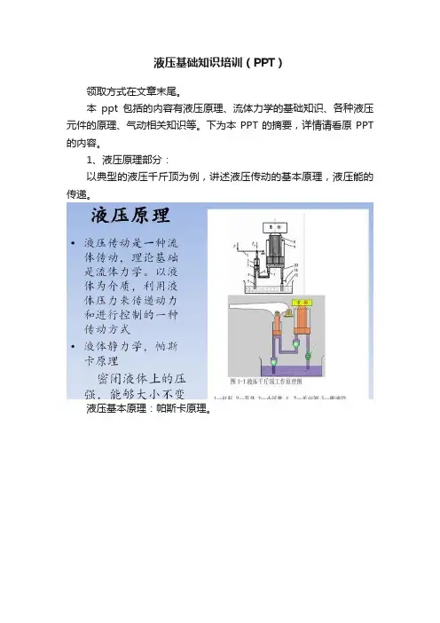
1、液压原理部分：
以典型的液压千斤顶为例，讲述液压传动的基本原理，液压能的传递。

液压基本原理：帕斯卡原理。

除此以外，还包括液压传动的流体力学基础，包括静力学方程、连续性方程、伯努利方程等。

2、液压元件
对常见的液压元件的工作原理和种类进行介绍。

动力元件：为液压系统提供液压能，包括齿轮泵、叶片泵、柱塞泵。

控制元件：包括压力控制阀、流量控制阀、方向控制阀。

执行元件：直接驱动负载做功。

3、气压传动的工作原理
领取方式：。