国际金融16

国际金融名词解释1、国际收支：是指一国在一定时期内全部对外经济往来的系统的货币记录。

P102、自主性交易：指个人和企业为某种自主性目的(比如追逐利润、旅游、汇款赡养亲友等)而从事的交易。

P243、补偿性交易：是指为弥补国际收支不平衡而发生的交易，比如为弥补国际收支逆差而向外国政府或国际金融机构借款、动用官方储备。

P244、马歇尔－勒纳条件：本币贬值会引起进出口商品价格变动，进而引起进出口商品的数量发生变动，最终引起贸易收支变动。

当出口商品的需求弹性和进口商品的需求弹性之和大于1时，贸易收支才能改善，它是本币贬值能带来国际收支改善的必要条件。

P375、J曲线效应：以时间为横轴，贸易收支为纵轴，本币贬值后贸易余额先向下变动，其后向上变动，贸易收支变化的曲线呈J形，因此，贬值对贸易收支改善的时滞效应，被称为J曲线效应。

P386、贸易条件：又称交换比价，是指出口商品单位价格指数与进口商品单位价格指数之间的比例。

P397、直接标价法：固定外国货币的数量，以本国货币表示这一固定数量的外国货币的价格，这称为外币的直接标价法。

8、间接标价法：固定本国货币的数量，以外国货币表示这一固定数量的外国货币的价格，从而间接地表示出外国货币的价格，这称为外币的间接标价法。

P549、名义汇率：汇率是一个国家的货币折算成另一个国家货币的比率，而名义汇率是指两国通货的相对价格。

10、实际汇率：某种表示货币实际竞争力和相对价格的指标11、均衡汇率：与宏观经济内外部均衡相一致的汇率，也就是内、外部均衡同时实现时决定的汇率。

12、购买力平价：两国货币的汇率主要由两国货币的购买力决定的机制。

P6613、一价定律：如果认为可贸易品的运输成本为零，则同种可贸易品在各个地区的价格应该是一致的，这种一致关系称作“一价定律”。

P6614、内部均衡：反映国内总供给等于国内总需求的状态。

P11115、外部均衡：在国内经济均衡发展，内部均衡实现基础上的国际收支平衡(内部均衡基础上的外部均衡)。

表1-2外汇汇率第一章课后习题答案要点具体内容Key Terms1.外汇答：外汇是以外币表示的，用以清偿国际间债权债务的一种支付手段。

外汇买卖是债权的转移，而外汇支付则是完成国际间债权债务的清偿。

因此，外汇的主要特征有：①外汇是以外币表示的金融资产。

任何以本国货币表示的信用工具、支付手段、有价证券等对本国人来说都不能称其为外汇。

②外汇必须是可以自由兑换成其他形式的，或以其他货币表示的资产。

如果某种资产在国际间的自由兑换受到限制则不能称其为外汇。

比如，有些国家的货币当局实行外汇管制，禁止本币在境内外自由兑换成其他国家的货币，以这种货币表示的各种支付工具也不能随时转换成其他货币表示的支付手段，那么这种货币及其标识的支付工具在国际上就不能称作外汇。

根据外汇定义可知，可兑换的外国货币（包括纸币、硬辅币等）是一种外汇资产。

但这只是外汇资产中最基本的一种形式，也是最狭义的外汇形式。

随着信用制度的发展，产生了许多其他形式的外汇资产，它们包括：外币有价证券，如政府债券、公司债券、股票等：外汇支付凭证，如外国汇票、本票、支票等；外币存款凭证，如银行存款凭证、邮政储蓄凭证等等。

2.汇率答：外汇汇率又称外汇汇价，是不同货币之间兑换的比率或比价，即用一种货币表示的另一种货币的价格。

汇率一般有三个价：买入价、卖出价和中间价。

买入价是银行向同业或客户买入外汇时所使用的汇率。

在直接标价法下，外币折合本币数量较少的汇率为买入价：釆用间接标价法时，本币折合外币数量较多的汇率为买入价。

卖出价是银行向同业或客户卖出外汇时所使用的汇率，采用直接标价法时，外币折合本币数量较多的汇率为卖出价：采用间接标价法时，本币折合外币数量较少的汇率为卖出价。

卖出价与买入价之间的差额即为银行买卖外汇的收益，一般为0.5%左右。

中间价为核算成本的参考价，属参考汇率。

在外汇市场上，如只报一个汇率，即为中间汇率。

3.直接标价法答：直接标价法是指以一定单位的外国货币为标准（1, 10（）, 1000（）等）来计算折合多少单位的本国货币。

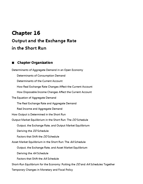
Chapter 16Output and the Exchange Ratein the Short RunChapter OrganizationDeterminants of Aggregate Demand in an Open EconomyDeterminants of Consumption DemandDeterminants of the Current AccountHow Real Exchange Rate Changes Affect the Current AccountHow Disposable Income Changes Affect the Current AccountThe Equation of Aggregate DemandThe Real Exchange Rate and Aggregate DemandReal Income and Aggregate DemandHow Output is Determined in the Short RunOutput Market Equilibrium in the Short Run: The DD ScheduleOutput, the Exchange Rate, and Output Market EquilibriumDeriving the DD ScheduleFactors that Shift the DD ScheduleAsset Market Equilibrium in the Short Run: The AA ScheduleOutput, the Exchange Rate, and Asset Market EquilibriumDeriving the AA ScheduleFactors that Shift the AA ScheduleShort-Run Equilibrium for the Economy: Putting the DD and AA Schedules Together Temporary Changes in Monetary and Fiscal PolicyChapter 16 Output and the Exchange Rate in the Short Run 77Monetary PolicyFiscal PolicyPolicies to Maintain Full EmploymentInflation Bias and Other Problems of Policy FormulationPermanent Shifts in Monetary and Fiscal PolicyA Permanent Increase in the Money SupplyAdjustment to a Permanent Increase in the Money SupplyA Permanent Fiscal Expansion78 Krugman/Obstfeld •International Economics: Theory and Policy, Eighth EditionMacroeconomic Policies and the Current AccountGradual Trade Adjustment and Current Account DynamicsThe J-CurveExchange-Rate Pass-Through and InflationBox: Exchange Rates and the Current AccountSummaryAppendix I: Intertemporal Trade and Consumption DemandAppendix II: The Marshall-Lerner Condition and Empirical Estimates of Trade Elasticities Online Appendix: The IS-LM and the DD-AA ModelChapter OverviewThis chapter integrates the previous analysis of exchange rate determination with a model of short-run output determination in an open economy. The model presented is similar in spirit to the classic Mundell-Fleming model, but the discussion goes beyond the standard presentation in its contrast of the effects of temporary versus permanent policies. The distinction between temporary and permanent policies allows for an analysis of dynamic paths of adjustment rather than just comparative statics. This dynamic analysis brings in the possibility of a J-curve response of the current account to currency depreciation. The chapter concludes with a discussion of exchange-rate pass-through, that is, the response of import prices to exchange rate movements.The chapter begins with the development of an open-economy fixed-price model (an online Appendix discusses the relationship between the IS-LM model and the analysis in this chapter). An aggregate demand function is derived using a Keynesian-cross diagram in which the real exchange rate serves as a shift parameter. A nominal currency depreciation increases output by stimulating exports and reducing imports, given foreign and domestic prices, fiscal policy, and investment levels. This yields a positively sloped output-market equilibrium (DD) schedule in exchange rate-output space. A negatively sloped asset-market equilibrium (AA) schedule completes the model. The derivation of this schedule follows from the analysis of previous chapters. For students who have already taken intermediate macroeconomics, you may want to point out that the intuition behind the slope of the AA curve is identical to that of the LM curve, with theChapter 16 Output and the Exchange Rate in the Short Run 79additional relationship of interest parity providing the link between the closed-economy LM curve and the open-economy AA curve. As with the LM curve, higher income increases money demand and raises the home-currency interest rate (given real balances). In an open economy, higher interest rates require currency appreciation to satisfy interest parity (for a given future expected exchange rate).The effects of temporary policies as well as the short-run and long-run effects of permanent policies can be studied in the context of the DD-AA model if we identify the expected future exchange rate with the long-run exchange rate examined in Chapters 14 and 15. In line with this interpretation, temporary policies are defined to be those which leave the expected exchange rate unchanged, while permanent policies are those which move the expected exchange rate to its new long-run level. As in the analysis in earlier chapters, in the long-run, prices change to clear markets (if necessary). While the assumptions concerning the expectational effects of temporary and permanent policies are unrealistic as an exact description of an economy, they are pedagogically useful because they allow students to grasp how differing market expectations about the duration of policies can alter their qualitative effects. Students may find the distinction between temporary and permanent, on the one hand, and between short run and long run, on the other, a bit confusing at first. It is probably worthwhile to spend a few minutes discussing this topic.80 Krugman/Obstfeld •International Economics: Theory and Policy, Eighth EditionBoth temporary and permanent increases in money supply expand output in the short run through exchange rate depreciation. The long-run analysis of a permanent monetary change once again shows how the well-known Dornbusch overshooting result can occur. Temporary expansionary fiscal policy raises output in the short run and causes the exchange rate to appreciate. Permanent fiscal expansion, however, has no effect on output even in the short run. The reason for this is that, given the assumptions of the model, the currency appreciation in response to permanent fiscal expansion completely “crowds out” exports. This is a consequence of the effect of a permanent fiscal expansion on the expected long-run exchange rate which shifts inward the asset-market equilibrium curve. This model can be used to explain the consequences of U.S. fiscal and monetary policy between 1979 and 1984. The model explains the recession of 1982 and the appreciation of the dollar as a result of tight monetary and loose fiscal policy.The chapter concludes with some discussion of real-world modifications of the basic model. Recent experience casts doubt on a tight, unvarying relationship between movements in the nominal exchange rate and shifts in competitiveness and thus between nominal exchange rate movements and movements in the trade balance as depicted in the DD-AA model. Exchange-rate pass-through is less than complete and thus nominal exchange rate movements are not translated one-for-one into changes in the real exchange rate. Also, the current account may worsen immediately after currency depreciation. This J-curve effect occurs because of time lags in deliveries and because of low elasticities of demand in the short run as compared to the long run. The chapter contains a discussion of the way in which the analysis of the model would be affected by the inclusion of incomplete exchange-rate pass-through and time-varying elasticities. Appendix II provides further information on trade elasticities with a presentation of the Marshall-Lerner conditions and a reporting of estimates of the impact, short-run and long-run elasticities of demand for international trade in manufactured goods for a number of countries.Answers to Textbook Problems1. A decline in investment demand decreases the level of aggregate demand for anylevel of the exchange rate. Thus, a decline in investment demand causes the DDcurve to shift to the left.2. A tariff is a tax on the consumption of imports. The demand for domestic goods, andthus the levelof aggregate demand, will be higher for any level of the exchange rate. This isdepicted in Figure 16.1 as a rightward shift in the output market schedule from DD to D'D'. If the tariff is temporary, thisis the only effect, and output will rise even though the exchange rate appreciates as the economymoves from Points 0 to 1. If the tariff is permanent, however, the long-run expected exchange rate appreciates, so the asset market schedule shifts to A'A'. Theappreciation of the currency is sharperin this case. If output is initially at full employment, then there is no change in output due to a permanent tariff.Chapter 16 Output and the Exchange Rate in the Short Run 81Figure 16.182 Krugman/Obstfeld •International Economics: Theory and Policy, Eighth Edition3. A temporary fiscal policy shift affects employment and output, even if thegovernment maintains a balanced budget. An intuitive explanation for this reliesupon the different propensities to consumeof the government and of taxpayers. If the government spends $1 more and finances this spendingby taxing the public $1 more, aggregate demand will have risen because thegovernment spends the entire $1, while the public reduces its spending by less than $1 (choosing to reduce its saving as well as its consumption). The ultimate effect on aggregate demand is even larger than this first round difference betweengovernment and public spending propensities, since the first round generatessubsequent spending. (Of course, currency appreciation still prevents permanent fiscal shifts from affecting output in our model.)4. A permanent fall in private aggregate demand causes the DD curve to shift inwardand to the left and, because the expected future exchange rate depreciates, the AA curve shifts outward and to the right. These two shifts result in no effect on output, however, for the same reason that a permanent fiscal expansion has no effect on output. The net effect is a depreciation in the nominal exchange rate and, because prices will not change, a corresponding real exchange rate depreciation. Amacroeconomic policy response to this event would not be warranted.5. Figure 16.2 can be used to show that any permanent fiscal expansion worsens thecurrent account.In this diagram, the schedule XX represents combinations of the exchange rate and income for which the current account is in balance. Points above and to the left of XX represent current account surplus, and points below and to the right representcurrent account deficit. A permanent fiscal expansion shifts the DD curve to D'D' and, because of the effect on the long-run exchange rate, the AA curve shifts to A'A'. The equilibrium point moves from 0, where the current account is in balance, to 1, where there is a current account deficit. If, instead, there was a temporary fiscal expansion of the same size, the AA curve would not shift and the new equilibrium would be at Point 2 where there is a current account deficit, although it is smaller than thecurrent account deficit at Point 1. Thus, a temporary increase in governmentspending causes the current account to decline by less than a permanent increase because there is no change in expectations with a temporary shock and thus the AA curve does not move.Chapter 16 Output and the Exchange Rate in the Short Run 83Figure 16.284 Krugman/Obstfeld •International Economics: Theory and Policy, Eighth Edition6. A temporary tax cut shifts the DD curve to the right and, in the absence ofmonetization, has no effect on the AA curve. In Figure 16.3, this is depicted as a shift in the DD curve to D'D', with the equilibrium moving from Points 0 to 1. If the deficit is financed by future monetization, the resulting expectedlong-run nominal depreciation of the currency causes the AA curve to shift to the right to A'A' which gives us the equilibrium Point 2. The net effect on the exchange rate is ambiguous, but output certainly increases more than in the case of a pure fiscal shift.Figure 16.37. A currency depreciation accompanied by a deterioration in the current accountbalance could be caused by factors other than a J-curve. For example, a fall inforeign demand for domestic products worsens the current account and also lowers aggregate demand, depreciating the currency. In termsof Figure 16.4, DD and XX undergo equal vertical shifts, to D'D' and X'X', respectively, resulting ina current account deficit as the equilibrium moves from Points 0 to 1. To detect a J-curve, one might check whether the prices of imports in terms of domestic goods rise when the currency is depreciating, offsetting a decline in import volume and a rise in export volume.Figure 16.48. The expansionary money supply announcement causes a depreciation in theexpected long-run exchange rate and shifts the AA curve to the right. This leads to an immediate increase in outputChapter 16 Output and the Exchange Rate in the Short Run 85and a currency depreciation. The effects of the anticipated policy action thus precede the policy’s actual implementation.9. The DD curve might be negatively sloped in the very short run if there is a J-curve,though the absolute value of its slope would probably exceed that of AA. This isdepicted in Figure 16.5. The effects of a temporary fiscal expansion, depicted as a shift in the output market curve to D'D', would not be altered since it would still expand output and appreciate the currency in this case (the equilibrium points moves from 0 to 1).Figure 16.5Monetary expansion, however, while depreciating the currency, would reduce output in the veryshort run. This is shown by a shift in the AA curve to A'A' and a movement in theequilibriumpoint from 0 to 2. Only after some time would the expansionary effect of monetary policy takehold (assuming the domestic price level did not react too quickly).10. The derivation of the Marshall-Lerner condition uses the assumption of a balancedcurrent account to substitute EX for (q⨯EX*). We cannot make this substitution when the current account is not initially zero. Instead, we define the variable z (q⨯EX*)/EX. This variable is the ratio of imports to exports, denominated in common units.When there is a current account surplus, z will be less than 1, and when there is acurrent account deficit, z will exceed 1. It is possible to take total derivatives of each side of the equation CA EX q EX * and derive a general Marshall-Lernercondition as n z n *z, where n and n* are as defined in the appendix. Thebalanced current account (z 1) Marshall-Lerner condition is a special case of this general condition. A depreciation is less likely to improve the current account thelarger its initial deficit when n* is less than 1. Conversely, a depreciation is more likely to cause an improvement in the current account the larger its initial surplus, again for values of n* less than 1.Figure 16.611. If imports constitute part of the CPI, then a fall in import prices due to anappreciation of the currency will cause the overall price level to decline. The fall in the price level raises real balances. As shown in Figure 16.6, the shift in the output market curve from DD to D'D' is matched by an inward shift of the asset marketequilibrium curve. If import prices are not in the CPI and the currency appreciation does not affect the price level, the asset market curve shifts to A"A" and there is no effect on output, even in the short run. If, however, the overall price level falls due to the appreciation, the shift in the asset market curve is smaller, to A'A', and the initial equilibrium point, Point 1, has higher output than the original equilibrium at Point 0.Over time, prices rise when output exceeds its long-run level, causing a shift in the asset market equilibrium curve from A'A' to A"A", which returns output to its long-run level.12. An increase in the risk premium shifts the asset market curve out and to the right, allelse equal.A permanent increase in government spending shifts the asset market curve in andto the right sinceit causes the expected future exchange rate to appreciate. A permanent rise ingovernment spending also causes the goods market curve to shift down and to the right since it raises aggregate demand. In the case where there is no risk premium, the new intersection of the DD and AA curves after a permanent increase ingovernment spending is at the full-employment level of output, since this is the only level consistent with no change in the long-run price level. In the case discussed in this question, however, the nominal interest rate rises with the increase in the risk premium. Therefore, output must also be higher than the original level of full-employment output; as compared to the case in the text, theAA curve does not shift by as much, so output rises.13. Suppose output is initially at full employment. A permanent change in fiscal policywill cause both the AA and DD curves to shift such that there is no effect on output.Now consider the case where the economy is not initially at full employment. Apermanent change in fiscal policy shifts the AA curve because of its effect on thelong-run exchange rate and shifts the DD curve because of its effect on expenditures.There is no reason, however, for output to remain constant in this case since its initial value is not equal to its long-run level, and thus an argument like the one in the text that shows the neutrality of permanent fiscal policy on output does not carrythrough. In fact, we might expect that an economy that begins in a recession (below Y f) would be stimulated back towards Y f by a positive permanent fiscal shock. If Y does rise permanently, we would expect a permanent drop in the price level (since Mis constant). This fall in P in the long run would move AA and DD both out. We could also consider the fact that in the case where we begin at full employment and there is no impact on Y, AA was shifting back due to the real appreciation necessitated by the increase in demand for home products (as a result of the increase in G). If there isa permanent increase in Y, there has also been a relative supply increase which canoffset the relative demand increase and weaken the need for a real appreciation.Because of this, AA would shift back by less. We do not know the exact effectwithout knowing how far the lines originally move (the size of the shock), but we do know that without the restriction that Y is unchanged in the long run, the argument in the text collapses, and we can have both short run and long run effects on Y.14. If some of the currency appreciation is temporary due to the current account effects,we will see a slightly different process after a permanent fiscal expansion. We would not necessarily still jump from Points 0 to 2 in Figure 16.2 above. We know that over time, the shift in consumption preferences away from the home good (due to the transfer of wealth to foreign consumers) will bring the DD curve back in some, this will cause a small depreciation in the future. Thus, the AA curve may not move in as far, leaving us with less appreciation immediately, but also with a small increase in GDP immediately. Eventually, the DD curve will move back a bit, bringing us back to full employment and with an appreciated currency (though less appreciated than inFigure 16.2).15. The text shows output cannot rise following a permanent fiscal expansion if output isinitially at its long-run level. Using a similar argument, we can show that outputcannot fall from its initial long-run level following a permanent fiscal expansion. A permanent fiscal expansion cannot have an effect on the long-run price level since there is no effect on the money supply or the long-run values of the domesticinterest rate and output. When output is initially at its long-run level, R equals R*, Y equals Y f and real balances are unchanged in the short run. If output did fall, there would be excess money supply and the domestic interest rate would have to fall, but this would imply an expected appreciation of the currency since the interestdifferential (R R *) would then be negative. This, however, could only occur if the currency appreciates in real terms as output rises and the economy returns to long-run equilibrium. This appreciation, however, would cause further unemployment, and output would not rise and return back to Y f. As with the example in the text, this contradiction is only resolved if output remains at Y f.16. It is difficult to see how government spending can rise permanently withoutincreasing taxes or how taxes can be cut permanently without cutting spending.Thus, a truly permanent fiscal expansion is difficult to envision. The one possiblescenario is if the government realized it was on a path to permanent surpluses and it could cut taxes without risking long-run imbalances. Because rational agents are aware the government has a long-run budget constraint, they may assume that any fiscal policy is actually temporary. This would mean that a “permanent” shockwould look just like a temporary one. This is quite similar to the discussion ofProblem 14 in this chapter.17. High inflation economies should have higher pass-through as price setters are used tomaking adjustments faster (menu costs fall over time as people learn how to change prices faster). Thus, a depreciation in a high inflation economy may see a rapidresponse of changing prices, but firms in a low inflation environment may be loathe to increase prices for fear of losing business given that their customersare not accustomed to price changes. In addition, a depreciation by a high inflation economy maybe more likely to have been caused by an increase in the money supply which would lead to price increases on its own anyway, so the pass-through would appear higher.。

《国际金融学》练习题一、判断题1、国际货币基金组织与世界银行集团就是世界上成员国最多、机构最庞大的国际金融机构。

( 对 )2、国际清算银行就是世界上成员国最多、机构最庞大国际金融机构。

( 错 )3、国际货币基金组织会员国提用储备部分贷款就是无条件的,也不需支付利息。

( 对 )4、国际货币基金组织会员国的投票权与其缴纳的份额成反比。

( 错 )5、国际货币基金组织的贷款只提供给会员国的政府机构。

( 对 )6、国际货币基金组织的贷款主要用于会员国弥补国际收支逆差。

( 错 )7、参加世界银行的国家必须就是国际货币基金组织的成员国。

( 对 )8、参加国际货币基金组织的成员国一定就是世界银行的成员国。

( 错 )9、被称为资本主义世界的第一个“黄金时代”的国际货币体系就是布雷顿森林体系。

( 错 )10、布雷顿森林协定包括《国际货币基金协定》与《国际复兴开发银行协定》。

( 对 )11、“特里芬两难”就是导致布雷顿森林体系崩溃的根本原因。

(对)12、牙买加体系就是以美元为中心的多元化国际储备体系( 对 )。

13、牙买加体系完全解决了“特里芬两难”。

( 错 )14、蒙代尔提出的汇率制度改革方案就是设立汇率目标区。

( 错 )15、威廉姆森提出的汇率制度改革方案就是恢复国际金本位制。

( 错 )16、欧洲支付同盟成立就是欧洲货币一体化的开端。

( 对 )17、《政治联盟条约》与《经济与货币联盟条约》,统称为“马斯特里赫特条约”,简称“马约”。

( 对 )18、《马约》关于货币联盟的最终要求就是在欧洲联盟内建立一个统一的欧洲中央银行并发行统一的欧洲货币。

( 对 )19、政府信贷的利率较低,期限较长,带有援助性质,但就是有条件。

( 对 )20、国际金融机构信贷的贷款利率通常要比私人金融机构的低,而且贷款条件非常宽松。

( 错 )21、在国际债务结构管理中,应避免尽量提高长期债务的比重,减少短期债务的比重。

( 对 )22、在国际债务的结构管理上,应尽量提高浮动利率债务的比重,减少固定利率债务的比重。

国际金融试题及答案一、单项选择题（每题1分，共10分）1. 国际金融中，汇率的标价方式通常有几种？A. 1种B. 2种C. 3种D. 4种2. 以下哪项不是国际收支平衡表的主要组成部分？A. 经常账户B. 资本账户C. 金融账户D. 贸易账户3. 外汇储备的主要作用是什么？A. 调节国际收支B. 稳定本币汇率C. 促进国际贸易D. 以上都是4. 汇率波动对以下哪个行业影响最大？A. 制造业B. 农业C. 服务业D. 旅游业5. 根据国际货币基金组织(IMF)的定义，SDR（特别提款权）是一种：A. 国际储备资产B. 国际支付手段C. 国际货币D. 国际债券6. 跨国公司在进行国际投资时，主要考虑的因素不包括：A. 政治风险B. 经济风险C. 汇率风险D. 个人偏好7. 国际金融市场中，短期资金的借贷通常发生在：A. 货币市场B. 资本市场C. 外汇市场D. 黄金市场8. 以下哪个不是国际金融危机的常见原因？A. 过度借贷B. 资产泡沫C. 政治不稳定D. 贸易顺差9. 国际货币体系的演变经历了哪些阶段？A. 金本位制、布雷顿森林体系、浮动汇率制A. 布雷顿森林体系、金本位制、浮动汇率制C. 浮动汇率制、金本位制、布雷顿森林体系D. 金本位制、浮动汇率制、布雷顿森林体系10. 国际金融监管机构中，负责制定全球银行监管标准的是：A. IMFB. 世界银行C. 巴塞尔委员会D. 国际清算银行二、多项选择题（每题2分，共10分）11. 国际金融市场的参与者包括：A. 各国中央银行B. 商业银行C. 投资银行D. 个人投资者12. 国际金融中，汇率的类型包括：A. 固定汇率B. 浮动汇率C. 爬行汇率D. 管理浮动汇率13. 国际投资的主要形式有：A. 直接投资B. 间接投资C. 股权投资D. 债券投资14. 国际金融风险管理的策略包括：A. 风险转移B. 风险规避C. 风险接受D. 风险控制15. 影响汇率变动的因素包括：A. 利率差异B. 通货膨胀率C. 政治稳定性D. 国际收支状况三、简答题（每题5分，共20分）16. 简述国际收支平衡表的构成及其意义。

新租赁准则IFRS16对租赁市场交易双方的影响引言：IFRS 16是国际金融报告准则第16号，是国际会计准则委员会（IASB）于2016年1月发布的最新的关于租赁会计处理的准则。

IFRS 16的实施标识着对租赁合同会计处理方式的重大改变，主要影响资产租赁及租赁债务的会计处理方法。

本文将分析新租赁准则IFRS 16对租赁市场交易双方（租赁人和出租人）的影响。

2. 营业成本的变化IFRS 16要求租赁人将租赁费用从营业成本中转向收益前利息、税项、折旧和摊销（EBITDA）中，这将导致租赁人的营业成本和利润水平的改变。

对于租赁人来说，由于租赁费用不再作为营业成本，所以可能会导致EBITDA的增加，从而提高公司的利润水平。

这可能会对公司的财务指标、报表分析和股东利益产生影响。

3. 现金流量的变化对于租赁人来说，由于租赁费用从营业成本中转移到EBITDA中，所以现金流量表中的经营活动现金流量将减少。

由于租赁人需要支付额外的租金（如租赁负债上的利息），使得租赁人的现金流量表中的融资活动现金流量和投资活动现金流量也会受到影响。

租赁人需要重新评估其现金流量的规划、财务管理和融资策略。

1. 出租合同的变化根据IFRS 16的要求，租赁人将租赁合同作为负债计入资产负债表中，出租人则将租金收入计入资产负债表中的利润和损益表。

这意味着出租人的财务报表将更准确地反映其租赁活动的收入水平。

对于出租人来说，由于合同负债的识别和计量，会使其租赁合同更加透明和可比较。

2. 风险管理的变化IFRS 16的实施要求出租人根据其对租赁人的不可取消性条款的评估，将租赁合同进行分类，并根据分类对租赁合同的披露要求进行不同的报告。

这将帮助出租人更好地管理与租赁活动相关的风险和收益，并提供更有利于投资者对公司业务的了解和评估的信息。

3. 合同谈判的变化对于出租人来说，由于IFRS 16的实施，租赁负债的计入资产负债表中将对其财务指标产生影响（如杠杆率、利息覆盖倍数等）。

判断题1、在间接标价法下,当外国货币数量减少时，称外国货币汇率下浮或贬值。

( ）2、本国资产减少，负债增加的项目应记入贷方。

（）3、补贴和关税政策属于支出增减型政策，而汇率政策属于支出转换型政策。

（）4、如果一国实行固定汇率制,其拥有的国际储备量可以相对较小。

（)6、消除国际收支逆差的措施之一是降低贴现率。

（)7、货币贬值不一定能改善一国的贸易收支.（）8、一般地说,利率较高的货币其远期汇率会呈现升水。

( ）9、布雷顿森林体系的两大支柱一是固定汇率制，二是政府干预制. （）10、如果一个投机者预测日元的汇率将上升，他通常的做法是买入远期的日元。

（)11、在纸币流通制度下,调节国际收支逆差的措施之一是削减财政开支和税收.（）12、贬值的弊端之一就是可能引起贬值国的国内通胀加剧，从而抵消了贬值的部分作用。

( ）13、国际收支平衡表中,储备资产项目为+12亿美元，则表示该国的国际储备资产增加了12亿美元.（）14、外汇银行标示的“买入价”即银行买入本币的价格；“卖出价”即银行卖出本币的价格。

（）15、外国投资者购买我国中国银行发行的日元债券, 对我国来讲属于资本流出，对外国来讲属于资本流入。

（）1．国际金本位制的最大缺点是国际经济和贸易的发展要受制于世界黄金产量的增长。

（√)2．资产减少,负债增加的项目应记入借方.（×）3．我国采用直接标价法,而美国采用间接标价法。

（√）5．贱卖贵买是套汇的基本原则。

（×）6．某投机者预期美元有贬值的可能，他就会做先买后卖的投机活动,称为“空头交易”。

(×）8．一般地说，利率较低的货币其远期汇率会呈现升水。

（√）9．通常所指的欧洲货币市场主要是指欧洲国家的金融市场。

（×）10．金融市场的发育程度越高，对国际储备的需求就越大。

（×）11．在纸币流通制度下，调节国际收支逆差的措施之一是削减财政开支。

（√)12．贬值的弊端之一就是可能引起贬值国的国内通胀加剧，从而抵消了贬值的部分作用。

金融16条原文解读1.加强金融监管，防范系统性风险。

解读：加强对金融机构的监管，规范金融市场秩序，防范出现系统性风险，保障金融市场的稳定运行。

2. 坚持稳健的货币政策，保持流动性合理充裕，维护金融稳定。

解读：坚持货币政策的稳健性，保证货币的供给和流动性的合理充裕，维护金融市场的稳定。

3. 坚决打好防范化解重大金融风险攻坚战。

解读：坚决打好防范和化解重大金融风险的攻坚战，发挥金融机构的作用，规范金融市场秩序，加强对风险的监控和防范。

4. 推动金融供给侧结构性改革，促进金融业转型升级。

解读：推动金融供给侧的结构性改革，促进金融业的转型升级，提高金融服务的质量和效率。

5. 深化金融市场改革，提高金融市场的自主性、市场化水平和国际化程度。

解读：深化金融市场改革，逐步提高金融市场的自主性、市场化水平和国际化程度，加强金融市场的监管和规范。

6. 推动金融创新，加强科技创新与金融服务的深度融合。

解读：推动金融创新，加强科技创新与金融服务的深度融合，推动金融服务的数字化、智能化发展。

7. 加强对金融消费者权益的保护，促进金融消费者合法权益得到有效维护。

解读：加强对金融消费者权益的保护，保障消费者的合法权益，维护金融市场的公正、公平、透明。

8. 推动绿色金融发展，促进经济可持续发展和生态文明建设。

解读：推动绿色金融的发展，促进经济可持续发展和生态文明建设，推动金融服务的绿色化、低碳化、环保化。

9. 推进金融对外开放，扩大金融业务对外开放程度。

解读：推进金融对外开放，扩大金融业务对外开放的程度，提高金融市场的国际竞争力。

10. 深入开展金融扶贫，加强金融服务乡村振兴和精准扶贫工作。

解读：深入开展金融扶贫，加强金融服务乡村振兴和精准扶贫工作，支持贫困地区和农村地区的经济发展。

11. 加强金融人才培养，提升金融从业人员素质和能力水平。

解读：加强金融人才培养，提高金融从业人员的素质和能力水平，适应金融市场的发展需求。

12. 建立健全金融风险防控体系，确保金融风险得到有效控制。

国际金融练习题（含答案一、单项选择题1、一国货币升值对其进出口收支产生何种影响（）A、出口增加，进口减少B、出口减少，进口增加C、出口增加，进口增加D、出口减少，进口减少2、汇率不稳有下浮趋势且在外汇市场上被人们抛售的货币是（）A、非自由兑换货币B、硬货币C、软货币D、自由外汇3、汇率波动受黄金输送费用的限制，各国国际收支能够自动调节，这种货币制度是（）A、浮动汇率制B、国际金本位制C、布雷顿森林体系D、混合本位制5、在采用直接标价的前提下，如果需要比原来更少的本币就能兑换一定数量的外国货币，这表明（）A、本币币值上升，外币币值下降，通常称为外汇汇率上升B、本币币值下降，外币币值上升，通常称为外汇汇率上升C、本币币值上升，外币币值下降，通常称为外汇汇率下降D、本币币值下降，外币币值上升，通常称为外汇汇率下降6、当一国经济出现通货膨胀和顺差时，为了内外经济的平衡，根据财政货币政策配合理论，应采取的措施是（）A、膨胀性的财政政策和膨胀性的货币政策B、紧缩性的财政政策和紧缩性的货币政策C、膨胀性的财政政策和紧缩性的货币政策D、紧缩性的财政政策和膨胀性的货币政策7、欧洲货币市场是（）A、经营欧洲货币单位的金融市场B、经营欧洲国家货币的金融市场C、欧洲国家国际金融市场的总称D、经营境外货币的国际金融市场8、国际债券包括（）A、固定利率债券和浮动利率债券B、外国债券和欧洲债券C、美元债券和日元债券D、欧洲美元债券和欧元债券9、一国国际收支顺差会使（）A、外国对该国货币需求增加，该国货币汇率上升B、外国对该国货币需求减少，该国货币汇率下跌C、外国对该国货币需求增加，该国货币汇率下跌D、外国对该国货币需求减少，该国货币汇率上升10、金本位的特点是黄金可以（）A、自由买卖、自由铸造、自由兑换B、自由铸造、自由兑换、自由输出入C、自由买卖、自由铸造、自由输出入D、自由流通、自由兑换、自由输出入11、根据财政政策配合的理论，当一国实施紧缩性的财政政策和货币政策，其目的在于（）A、克服该国经济的通货膨胀和国际收支逆差B、克服该国经济的衰退和国际收支逆差C、克服该国通货膨胀和国际收支顺差D、克服该国经济衰退和国际收支顺差12、资本流出是指本国资本流到外国，它表示（）A、外国对本国的负债减少B、本国对外国的负债增加C、外国在本国的资产增加D、外国在本国的资产减少13、目前，我国人民币实施的汇率制度是（）A、固定汇率制B、弹性汇率制C、有管理浮动汇率制D、钉住汇率制14、若一国货币汇率高估，往往会出现（）A、外汇供给增加，外汇需求减少，国际收支顺差B、外汇供给减少，外汇需求增加，国际收支逆差C、外汇供给增加，外汇需求减少，国际收支逆差D、外汇供给减少，外汇需求增加，国际收支顺差15、从长期讲，影响一国货币币值的因素是（）A、国际收支状况B、经济实力C、通货膨胀D、利率高低16、所谓外汇管制就是对外汇交易实行一定的限制，目的是（）A、防止资金外逃B、限制非法贸易C、奖出限入D、平衡国际收支、限制汇价17、持有一国国际储备的首要用途是（）A、支持本国货币汇率B、维护本国的国际信誉C、保持国际支付能力D、赢得竞争利益18、当国际收支的收入数字大于支出数字时，差额则列入( )以使国际收支人为地达到平衡。

国际金融学习题答案国际金融学习题答案第一章2．国际收支总差额是（D ）2008.1A．经常账户差额与资本账户差额之和B．经常账户差额与长期资本账户差额之和C．资本账户差额与金融账户差额之和D．经常账户差额、资本账户差额、金融账户差额、净差错与遗漏四项之和13.国际收支是统计学中的一个（B ）2009.1A.存量概念B.流量概念C.衡量概念D.变量概念15.本国居民因购买和持有国外资产而获得的利润、股息及利息应记入（ A ）2009.1A.经常账户B.资本账户C.金融账户D.储备资产账户1.按照《国际收支手册》第五版的定义，IMF判断个人居民的标准是（ D ）2009.10A.国籍标准C.法律标准B.时间标准D.住所标准2.保险费记录在经常项目中的（B ）2009.10A.货物B.服务C.收益D.经常转移2.广义国际收支建立的基础是（C ）2010.1A.收付实现制B.国际交易制C.权责发生制D.借贷核算制1.国际收支平衡表的实际核算与编制过程，没有完全按照复式借贷记账法去做，由此导致了平衡表中什么项目的产生?( D )2010.10A.经常项目C.平衡项目B.资产项目D.错误与遗漏2.政府贷款及出口信贷记录在金融账户中的哪一个项目?( D ) 2010.10A.直接投资B.间接投资C.证券投资D.其他投资1.我国企业在香港发行股票所筹集的资金应记入国际收支平衡表的( C )2011.1A.经常账户B.资本账户C.金融账户D.储备账户2.我国国际收支平衡表中经常账户的借方记录( C ) 2011.1A.商品的进出口额100万元B.好莱坞电影大片的进口额20万美元C.对外经济援助50万美元D.外国人到中国旅游支出2万美元16.我国某企业获得外国汽车专利的使用权。

该项交易应记入国际收支平衡表的( B ) 2011.1A.贸易收支B.服务收支C.经常转移收支D.收入收支13．政府间的经济与军事援助记录在（A ）2008.10A．经常账户B．资本账户C．金融账户D．储备资产账户28.国际收支差额等于经常账户差额加上资本与金融账户差额。