QSplat A Multiresolution Point Rendering System for Large Meshes
- 格式:pdf
- 大小:3.12 MB
- 文档页数:10

基于外存八叉树的三维激光点云实时渲染技术邱炎;梁玉斌;崔铁军【摘要】为了解决海量点云数据的实时渲染问题,采用基于外存储器构建细节层次八叉树索引结构的方法用于三维点云数据实时渲染,并用8G内存的普通计算机对天津师范大学教学区10.2 GB的扫描点云数据进行实验验证.结果表明:实时渲染时的帧率在16f/s上下浮动,且无明显延迟,表明该方法支持超过内存容量的三维激光扫描点云数据的实时渲染.【期刊名称】《天津师范大学学报(自然科学版)》【年(卷),期】2017(037)003【总页数】4页(P58-61)【关键词】实时渲染;八叉树;层次细节模型;三维激光点云数据【作者】邱炎;梁玉斌;崔铁军【作者单位】天津师范大学城市与环境科学学院,天津300387;天津师范大学城市与环境科学学院,天津300387;天津师范大学城市与环境科学学院,天津300387【正文语种】中文【中图分类】P237三维激光扫描是目前获取地理空间数据的重要手段之一[1],与传统测量手段相比,三维激光扫描测量技术可以快速、直接地获取目标物表面大量三维测量数据[2].随着三维激光扫描技术的深入应用,三维激光扫描获取的点云数据量越来越大,大规模三维激光扫描点云的实时渲染已成为点云数据交互式处理的瓶颈问题.近年来,国内外学者针对海量激光扫描点云数据的实时渲染开展了大量研究.Levoy和Whitted[3-4]首次引入基于点的三维模型渲染方法,该模型可以表达出任意连续的三维表面,用于海量数据的编辑和渲染.Rusinkiewicz等[5]提出了可用于大规模三维数字模型实时渲染的QSplat系统,该系统的核心算法将采样点存储在层次外包球的内部,在渲染阶段将基于点的渲染系统与基于视角的多层金字塔模型相结合,实现数据的实时渲染.Martinez-Rubi等[6]基于WebGL实现了海量点云数据的网络可视化,该研究使用多分辨率的八叉树对点云进行渲染,为减少构建八叉树所耗费的时间,将整体区域根据一定规则划分为多个子单元,并对每个子单元构建八叉树,最终根据所有八叉树中节点的空间范围将多个八叉树进行合并.李婕[7]提出一种针对车载激光扫描点云数据的管理与可视化方法,该方法使用虚拟内存技术和快速显示技术处理点云数据,给出了点云分块索引模型的数据组织方法,实现了百万数量级点云数据的可视化[8].张会霞[9]提出一种基于数据库的点云管理方法,实现了点云数据的分块组织及检索.陈驰等[10]提出一种车载激光扫描点云数据的快速可视化方法,采用双层四叉树索引方法实现激光点云数据的管理与动态调度,从而做到千万数量级车载点云数据的可视化.虽然近年来国内外研究者对三维激光扫描点云数据的组织管理和实时渲染进行了大量研究,但大部分研究中点云数据的规模为千万数量级,当点云数据量进一步扩大,渲染方法的扩展性就成为实时渲染的关键.因此,针对超过计算机内存容量的三维激光扫描点云,本研究提出一种基于外存八叉树的实时渲染方法,以期用于大规模三维激光扫描点云数据的可视化和交互式处理.基于外存八叉树的大规模三维激光扫描点云实时渲染主要包括海量点云数据预处理和基于外存八叉树的细节层次实现两大部分.具体操作步骤为:首先,将大规模点云数据划分为多个点云分块,每个分块包含一定数量的扫描点;其次,以最近邻点数为阈值滤除每个点云分块中的孤立点;再次,遍历经过去噪的点云分块,统计测区覆盖的空间范围;最后,再次读取经过去噪的点云分块,在外存储器上建立不同细节层次的八叉树索引结构.1.1 海量点云数据的预处理海量点云数据的预处理包括点云数据的分块和点云去噪两部分.海量点云数据的数据量通常超过一般计算机的内存容量,因此无法直接将全部点云数据读入内存进行处理.点云数据的分块处理将全部点云数据划分为多个较小的点云分块,每个点云分块包含一定数量的扫描点,可以直接读入内存进行处理.建筑室内外场景中常常存在玻璃等镜面反射对象,镜面反射将引起噪声扫描点.噪点则会造成测区外包盒(bounding box)计算错误,从而导致最终生成错误的八叉树索引结构.因此,在数据预处理阶段必须进行点云去噪.扫描点由激光扫描仪顺序扫描获得,因而同一个点云分块中的扫描点通常在空间中彼此邻近,而噪点通常以孤立点形式存在.因此,通过读取每个分块点云文件,构建k-d tree,在给定近邻点数的基础上计算近邻点到邻域中心的平均距离和标准差,如果当前点与邻域中心的距离超出平均距离一个标准差,则将该点标记为噪点并从数据中剔除.1.2 基于外存八叉树的细节层次实现遍历所有经过去噪的点云文件,统计得到测区覆盖的空间范围.依次读取经过去噪的点云文件,根据计算得到的外包盒空间范围,然后在外存储器上建立不同细节层次的八叉树索引结构.1.2.1 八叉树索引本研究基于八叉树对点云数据进行三维空间索引,结构示意图如图1所示.图1中,八叉树的每个节点代表一个长方体空间,当存储点云数据时,预先设定八叉树的最大递归深度和节点最小容纳点数.索引结构以迭代方式构建,通过不断读入点云分块文件,将其划分到所属的八叉树节点.如果节点包含的点数超过预先设定的最小容纳点数,则将该节点进行剖分.当构建的八叉树的深度达到预先设定的最大递归深度时,不再进行节点剖分.有子节点的节点称为内节点或组节点,叶节点没有子节点[11].对于超出内存容量的点云数据,通过在外部存储器上构建数据索引结构,以避免海量数据实时渲染受物理内存容量的限制.首先,遍历所有经过去噪的点云文件,计算覆盖测区的外包盒的空间范围.其次,依次读取去噪后的点云文件,根据外包盒的空间范围,利用读入的扫描数据在外存储器上建立和更新统一的八叉树索引结构.待全部点云文件遍历完毕,即完成索引结构的构建.1.2.2 细节层次实现细节层次(level of detail,LOD)技术利用几何体包围盒计算观察者与物体的距离,使用户可以更高效地渲染处于不同细节层次上的物体[12].八叉树的根节点对应测区全部的点云数据,通过逐级对内节点进行细分,使得不同深度的节点对应地物对象的不同细节层次.根节点上的数据粒度最大,节点的粒度由上至下逐层减小,同一深度上不同节点的数据粒度相同,细节逐渐丰富.在实现上,每一个节点对应一个磁盘文件.通过细分,每个节点存储的点云数据量将保持在一定的范围内.此外,节点数据以二进制文件存储,可以进一步减少所占用的存储空间.当进行点云数据的实时渲染时,在有效观察范围内的节点被快速确定,这些节点对应的点云数据将从磁盘载入进行显示;当节点处于观察范围之外时,对应的数据将从内存移除,从而实现点云数据的动态调度和显示.图2显示了一个LOD节点及其子节点,当节点处于有效观察范围之内时,则显示该子节点.本研究实验区为天津师范大学教学区,点云数据利用RIEGL VZ-1000型三维激光扫描仪对地面进行静态测量获取.通过RTK测量的控制点对点云数据进行绝对定向,每个站点云数据经过初步处理后仅保留建筑点云数据用于实验.融合后的点云数据以pts格式文本文件保存,文件大小为10.2 GB,共包含192 132 546个激光扫描点,数据文件记录每个点的三维坐标和反射强度值.实验的硬件环境为配置有Intel Core i5-5200U处理器、8G内存和GeForce 940M显卡的笔记本电脑,操作系统为Ubuntu 15.04.实验方法基于C++,点云去噪、基于外存的数据调度和三维数据渲染子程序均依赖PCL(Point Cloud Library)和Open Scene Graph 库.预处理程序以数据流的方式读取点云数据,将全部点云数据以1 000万点/块划分为20个点云分块文件,程序耗时19 min44 s.点云去噪程序中近邻点数设为50,去噪用时21 min13 s,程序自动剔除13 517个噪点.最终进行渲染的点数为192 119 029个.在外存储器上建立不同细节层次八叉树索引结构时,八叉树的深度选择直接决定了渲染效率,随着深度的增加,渲染效果更加流畅,同时需要的内存空间也越大,若深度超过合适的值,效率会大大降低.本研究对不同深度八叉树索引结构的运算结果进行对比,随着深度的增加,建树程序消耗内存增大,所耗时间增加,但渲染程序消耗内存减小,所耗时间减少.综合考虑建立索引结构的程序运行时消耗的最大内存及用时、渲染程序运行时耗费的最大内存、数据载入耗时以及渲染帧率等因素,实验显示八叉树的最大深度设置为8时,可以在内存足以支撑程序运行的前提下得到最大的漫游帧率,从而实现最流畅的渲染效果.建立索引结构的程序运行时消耗的最大内存为1.2 GB,程序用时28 min 53 s.渲染程序运行时耗费的最大内存为1.4 GB,数据载入耗时为13 s.实时渲染时帧率在16 f/s上下浮动,无明显延迟.点云数据使用强度值进行渲染,渲染效果如图3所示.实时渲染程序支持对点云数据的放大缩小、全图、旋转和漫游等操作.利用本研究算法与点云处理的商业软件RISCAN PRO对相同数据进行渲染,实验显示RISCAN PRO无法加载10.2 G的实验数据,因而将扫描点数减少至40 570 418,数据文件大小为1.9 G.对2种方法的渲染性能进行比较,结果如表1所示,其中RISCAN PRO软件将扫描点数据直接读入内存进行渲染.由表1可以看出,在相同的硬件环境下,基于外存八叉树的渲染程序在运行时最大内存消耗为262 M,而使用RISCAN PRO软件进行渲染的最大内存消耗为310 M.数据载入耗时指从渲染程序开始加载点云数据到数据在计算机屏幕上完全显示出来所消耗的时间,本研究渲染程序载入数据的耗时为16 s,少于RISCAN PRO 软件的24 s.图4为本研究方法与RISCAN PRO软件在数据漫游帧率方面的比较结果.由图4可知,在数据显示速度方面,基于外存八叉树渲染方法的帧率明显大于RISCAN PRO软件的帧率,且渲染效果更为平滑流畅.本研究提出一种支持海量点云数据实时渲染的技术方法,分别利用点云数据分块实现了大规模点云的分治;点云去噪有效避免了因噪声导致的八叉树外包盒计算错误的问题;基于外存八叉树的索引结构则实现了细节层次模型,是海量点云实时渲染的关键.实验结果表明,本研究方法实现了对超过内存容量的三维激光扫描点云的实时渲染.该技术方法对硬件的要求不高,具有一定的实用价值.八叉树最优深度的自适应计算和点云数据的并行处理是后续研究的重点,这些研究的开展有望进一步提高数据处理系统的自动化程度,节省点云数据的处理时间.【相关文献】[1]李清泉,李必军.激光雷达测量技术及其应用研究[J].武汉测绘科技大学学报,2000,25(5):387-392. LI Q Q,LI B J.Research on laser range scanning and its application[J]. Journal of Wuhan Technical University of Surveying and Mapping,2000,25(5):387-392(in Chinese).[2]李必军,方志祥,任娟.从激光扫描数据中进行建筑物特征提取研究[J].武汉大学学报:信息科学版,2003,28(1):65-70. LI B J,FANG Z X,REN J.Extraction of building′s feature from laser scanning data[J].Geomatics and Information Science of Wuhan University,2003,28(1):65-70(in Chinese).[3]LEVOY M,WHITTED T.The use of points as a display primitive[R]. University of North Carolina,Department of Computer Science,1985.[4]LEVOY M,PULLI K,CURLESS B,et al.The digital Michelangelo project:3D scanning of large statues[C]//Proceedings of the 27th Annual Conference on Computer Graphics and Interactive Techniques.ACM Press/Addison-Wesley Publishing Co,2000:131-144.[5]RUSINKIEWICZ S,LEVOY M.QSplat:A multiresolution point rendering system for large meshes[C]//Proceedings of the 27th Annual Conference on Computer Graphics and Interactive Techniques.ACM Press/ Addison-Wesley Publishing Co,2000:343-352. [6]MARTINEZ-RUBI O,KLEIJN M D,VERHOEVEN S,et ing modular 3D digital earth applications based on point clouds for the study of complex sites[J].International Journal of Digital Earth,2016,9(12):1135-1152.[7]李婕.三维海量激光数据管理及可视化研究[D].北京:首都师范大学,2009. LI J.Massive Three-dimensional Laser Data Management and VisualizationResearch[D].Beijing:CapitalNormalUniversity,2009(inChinese).[8]徐鹏.海量三维点云数据的组织与可视化研究[D].南京:南京师范大学,2013. XU P.Massive Three-dimensional Point Cloud Management and VisualizationResearch[D].Nanjing:NanjingNormalUniversity,2013(inChinese).[9]张会霞.基于八叉树的点云数据的组织与可视化[J].太原师范学院学报:自然科学版,2011,10(3):128-132. ZHANG H X.The organization and visualization of point cloud data based on the octree[J].Journal of Taiyuan Normal University:Natural Science Edition,2011,10(3):128-132(in Chinese).[10]陈驰,王珂,徐文学,等.海量车载激光扫描点云数据的快速可视化方法[J].武汉大学学报:信息科学版,2015,40(9):1163-1168. CHEN C,WANG K,XU W X,et al.Real-time visualizing of massive vehicle-borne laser scanning point clouds[J].Geomatics and Information ScienceofWuhanUniversity,2015,40(9):1163-1168(inChinese). [11]ELSEBERG J,BORRMANN D,NÜCHTER A.One billion points in the cloud-an octree for efficient processing of 3D laser scans[J].ISPRS Journal of Photogrammetry and Remote Sensing,2013,76:76-88.[12]CLARK J H.Hierarchical geometric models for visible surfacealgorithms[J].Communications of the ACM,1976,19(10):547-554.。

第X章曲面快速重建(QUICK SURFACE RECONSTRUCTION)CA TIA V5 曲面快速重建(QUICK SURFACE RECONSTRUCTION)模块为重建不论是否具有机械几何特征的曲面提供了一种快捷易用的手段。
曲面快速重建(以下简称QSR)不仅可以构造诸如不具有平面、圆柱面和倒圆角特征的自由曲面,还可以构造包括自由曲面在内的其他具有机械特征如凸台、加强筋、斜度和平坦区域的特征曲面。
使用QSR模块可以直接依据点云数据重建曲面,也可以将原有实体修改后通过数字化处理成点云数据利用QSR重建原有的CAD模型上需修改的曲面。
QSR模块可以让设计者决定是注重重建曲面的效力还是重建曲面质量或两者都综合考虑以满足不同需求。
QSR构造的曲面还可以有参数以适应修改的需要。
x.1 相关的图标菜单CA TIA V5的曲面快速重建模块由如下图标菜单组成:点云编辑菜单(Cloud Edition)、扫描线创建菜单(Scan Creation)、曲线创建菜单(Curves Creation)、轮廓清理菜单(Clean Contour)、曲面创建菜单(Surface Creation)、几何操作菜单(Operations)、变换菜单(Transformations)以及分析菜单(Analysis)。
x.1.1 点云编辑菜单(Cloud Edition)Activate 激活点云x.1.2 扫描线创建菜单(Scan Creation)Project Curves 创建投影扫描线Planar Sections 创建平面截面扫描线x.1.3 曲线创建菜单(Curves Creation)3D curve 创建空间曲线Curve from Scans 由扫描线创建曲线Intersection 创建交线Projection 创建投影线x.1.4 轮廓清理菜单(Clean Contour)Clean Contour轮廓清理x.1.5 曲面创建菜单(Surface Creation)Basic Surface Recognition 特征曲面识别Power Fit 智能拟合Loft Surface 创建放样曲面x.1.6 几何操作菜单(Operations)Join合并几何元素Extrapolate延长曲线/曲面Split 切割曲面或线框元素Trim 修剪曲面或线框元素Curves Slice 曲线分段Edge Fillet曲面棱线倒圆x.1.7 变换菜单(Transformations)Translate移动几何体Rotate转动几何体Scale缩放几何体Symmetry对称几何体x.1.8 分析菜单(Analysis)Curvature Analysis曲率分析Slope Analysis 斜度分析Distance Analysis 距离分析Connect Checker 曲面连接性检查x.1.9 点云显示菜单(Cloud Display Options) Cloud Display Options 点云显示x.2 QSR功能介绍本节将详细地介绍相关的功能及各功能在实际造型中的应用。

CAD快捷键命令命令大全-- CAD绘图命令CAD绘图命令#3D 创建三维多边形网格对象3DARRAY 创建三维阵列3DCLIP 启用交互式三维视图并打开“调整剪裁平面”窗口3DCORBIT 启用交互式三维视图并允许用户设置对象在三维视图中连续运动3DDISTANCE 启用交互式三维视图并使对象显示得更近或更远3DFACE 创建三维面3DMESH 创建自由格式的多边形网格3DORBIT 控制在三维空间中交互式查看对象3DPAN 启用交互式三维视图并允许用户水平或垂直拖动视图3DPOLY 在三维空间中使用“连续”线型创建由直线段组成的多段线3DSIN 输入3D Studio (3DS) 文件3DSOUT 输出3D Studio (3DS) 文件3DSWIVEL 启用交互式三维视图模拟旋转相机的效果3DZOOM 启用交互式三维视图使用户可以缩放视图AABOUT 显示关于AutoCAD 的信息ACISIN 输入ACIS 文件ACISOUT 将AutoCAD 实体对象输出到ACIS 文件中ADCCLOSE 关闭AutoCAD 设计中心ADCENTER 管理内容ADCNAVIGATE 将AutoCAD 设计中心的桌面引至用户指定的文件名、目录名或网络路径ALIGN 在二维和三维空间中将某对象与其他对象对齐AMECONVERT 将AME 实体模型转换为AutoCAD 实体对象APERTURE 控制对象捕捉靶框大小APPLOAD 加载或卸载应用程序并指定启动时要加载的应用程序ARC 创建圆弧AREA 计算对象或指定区域的面积和周长ARRAY 创建按指定方式排列的多重对象副本ARX 加载、卸载和提供关于ObjectARX 应用程序的信息ATTDEF 创建属性定义ATTDISP 全局控制属性的可见性ATTEDIT 改变属性信息ATTEXT 提取属性数据ATTREDEF 重定义块并更新关联属性AUDIT 检查图形的完整性BBACKGROUND 设置场景的背景效果BASE 设置当前图形的插入基点BHATCH 使用图案填充封闭区域或选定对象BLIPMODE 控制点标记的显示BLOCK 根据选定对象创建块定义BLOCKICON 为R14 或更早版本创建的块生成预览图像BMPOUT 按与设备无关的位图格式将选定对象保存到文件中BOUNDARY 从封闭区域创建面域或多段线BOX 创建三维的长方体BREAK 部分删除对象或把对象分解为两部分BROWSER 启动系统注册表中设置的缺省Web 浏览器CCAL 计算算术和几何表达式的值CAMERA 设置相机和目标的不同位置CHAMFER 给对象的边加倒角CHANGE 修改现有对象的特性CHPROP 修改对象的颜色、图层、线型、线型比例因子、线宽、厚度和打印样式CIRCLE 创建圆CLOSE 关闭当前图形COLOR 定义新对象的颜色COMPILE 编译形文件和Postscript 字体文件CONE 创建三维实体圆锥CONVERT 优化AutoCAD R13 或更早版本创建的二维多段线和关联填充COPY 复制对象COPYBASE 带指定基点复制对象COPYCLIP 将对象复制到剪贴板COPYHIST 将命令行历史记录文字复制到剪贴板COPYLINK 将当前视图复制到剪贴板中,以使其可被链接到其他OLE 应用程序CUTCLIP 将对象复制到剪贴板并从图形中删除对象CYLINDER 创建三维实体圆柱DDBCCLOSE 关闭“数据库连接”管理器DBCONNECT 为外部数据库表提供AutoCAD 接口DBLIST 列出图形中每个对象的数据库信息DDEDIT 编辑文字和属性定义DDPTYPE 指定点对象的显示模式及大小DDVPOINT 设置三维观察方向DELAY 在脚本文件中提供指定时间的暂停DIM 和DIM1 进入标注模式DIMALIGNED 创建对齐线性标注DIMANGULAR 创建角度标注DIMBASELINE 从上一个或选定标注的基线处创建线性、角度或坐标标注DIMCENTER 创建圆和圆弧的圆心标记或中心线DIMCONTINUE 从上一个或选定标注的第二尺寸界线处创建线性、角度或坐标标注DIMDIAMETER 创建圆和圆弧的直径标注DIMEDIT 编辑标注DIMLINEAR 创建线性尺寸标注DIMORDINATE 创建坐标点标注DIMOVERRIDE 替换标注系统变量DIMRADIUS 创建圆和圆弧的半径标注DIMSTYLE 创建或修改标注样式DIMTEDIT 移动和旋转标注文字DIST 测量两点之间的距离和角度DIVIDE 将点对象或块沿对象的长度或周长等间隔排列DONUT 绘制填充的圆和环DRAGMODE 控制AutoCAD 显示拖动对象的方式DRAWORDER 修改图像和其他对象的显示顺序DSETTINGS 指定捕捉模式、栅格、极坐标和对象捕捉追踪的设置DSVIEWER 打开“鸟瞰视图”窗口DVIEW 定义平行投影或透视视图DWGPROPS 设置和显示当前图形的特性DXBIN 输入特殊编码的二进制文件EEDGE 修改三维面的边缘可见性EDGESURF 创建三维多边形网格ELEV 设置新对象的拉伸厚度和标高特性ELLIPSE 创建椭圆或椭圆弧ERASE 从图形中删除对象EXPLODE 将组合对象分解为对象组件EXPORT 以其他文件格式保存对象EXPRESSTOOLS 如果已安装AutoCAD 快捷工具但没有运行,则运行该工具EXTEND 延伸对象到另一对象EXTRUDE 通过拉伸现有二维对象来创建三维原型FFILL 控制多线、宽线、二维填充、所有图案填充和宽多段线的填充FILLET 给对象的边加圆角FILTER 创建可重复使用的过滤器以便根据特性选择对象FIND 查找、替换、选择或缩放指定的文字FOG 控制渲染雾化GGRAPHSCR 从文本窗口切换到图形窗口GRID 在当前视口中显示点栅格GROUP 创建对象的命名选择集HHATCH 用图案填充一块指定边界的区域HATCHEDIT 修改现有的图案填充对象HELP (F1) 显示联机帮助HIDE 重生成三维模型时不显示隐藏线HYPERLINK 附着超级链接到图形对象或修改已有的超级链接HYPERLINKOPTIONS 控制超级链接光标的可见性及超级链接工具栏提示的显示IID 显示位置的坐标IMAGE 管理图像IMAGEADJUST 控制选定图像的亮度、对比度和褪色度IMAGEATTACH 向当前图形中附着新的图像对象IMAGECLIP 为图像对象创建新剪裁边界IMAGEFRame 控制图像边框是显示在屏幕上还是在视图中隐藏IMAGEQUALITY 控制图像显示质量IMPORT 向AutoCAD 输入多种文件格式INSERT 将命名块或图形插入到当前图形中INSERTOBJ 插入链接或嵌入对象INTERFERE 用两个或多个三维实体的公用部分创建三维组合实体INTERSECT 用两个或多个实体或面域的交集创建组合实体或面域并删除交集以外的部分ISOPLANE 指定当前等轴测平面LLAYER 管理图层LAYOUT 创建新布局和重命名、复制、保存或删除现有布局LAYOUTWIZARD 启动“布局”向导,通过它可以指定布局的页面和打印设置LEADER 创建一条引线将注释与一个几何特征相连LENGTHEN 拉长对象LIGHT 处理光源和光照效果LIMITS 设置并控制图形边界和栅格显示LINE 创建直线段LINETYPE 创建、加载和设置线型LIST 显示选定对象的数据库信息LOAD 加载形文件,为SHAPE 命令加载可调用的形LOGFILEOFF 关闭LOGFILEON 命令打开的日志文件LOGFILEON 将文本窗口中的内容写入文件LSEDIT 编辑配景对象LSLIB 管理配景对象库LSNEW 在图形上添加具有真实感的配景对象,例如树和灌木丛LTSCALE 设置线型比例因子LWEIGHT 设置当前线宽、线宽显示选项和线宽单位MMASSPROP 计算并显示面域或实体的质量特性MATCHPROP 把某一对象的特性复制给其他若干对象MATLIB 材质库输入输出MEASURE 将点对象或块按指定的间距放置MENU 加载菜单文件MENULOAD 加载部分菜单文件MENUUNLOAD 卸载部分菜单文件MINSERT 在矩形阵列中插入一个块的多个引用MIRROR 创建对象的镜像副本MIRROR3D 创建相对于某一平面的镜像对象MLEDIT 编辑多重平行线MLINE 创建多重平行线MLSTYLE 定义多重平行线的样式MODEL 从布局选项卡切换到模型选项卡并把它置为当前MOVE 在指定方向上按指定距离移动对象MSLIDE 为模型空间的当前视口或图纸空间的所有视口创建幻灯片文件MSPACE 从图纸空间切换到模型空间视口MTEXT 创建多行文字MULTIPLE 重复下一条命令直到被取消MVIEW 创建浮动视口和打开现有的浮动视口MVSETUP 设置图形规格NNEW 创建新的图形文件OOFFSET 创建同心圆、平行线和平行曲线OLELINKS 更新、修改和取消现有的OLE 链接OLESCALE 显示“OLE 特性”对话框OOPS 恢复已被删除的对象OPEN 打开现有的图形文件OPTIONS 自定义AutoCAD 设置ORTHO 约束光标的移动OSNAP 设置对象捕捉模式PPAGESETUP 指定页面布局、打印设备、图纸尺寸,以及为每个新布局指定设置PAN 移动当前视口中显示的图形PARTIALOAD 将附加的几何图形加载到局部打开的图形中PARTIALOPEN 将选定视图或图层中的几何图形加载到图形中PASTEBLOCK 将复制的块粘贴到新图形中PASTECLIP 插入剪贴板数据PASTEORIG 使用原图形的坐标将复制的对象粘贴到新图形中PASTESPEC 插入剪贴板数据并控制数据格式PCINWIZARD 显示向导,将PCP 和PC2 配置文件中的打印设置输入到“模型”选项卡或当前布局PEDIT 编辑多段线和三维多边形网格PFACE 逐点创建三维多面网格PLAN 显示用户坐标系平面视图PLINE 创建二维多段线PLOT 将图形打印到打印设备或文件PLOTSTYLE 设置新对象的当前打印样式,或者选定对象中已指定的打印样式PLOTTERMANAGER 显示打印机管理器,从中可以启动“添加打印机”向导和“打印机配置编辑器”POINT 创建点对象POLYGON 创建闭合的等边多段线PREVIEW 显示打印图形的效果PROPERTIES 控制现有对象的特性PROPERTIESCLOSE 关闭“特性”窗口PSDRAG 在使用PSIN 输入Postscript 图像并拖动到适当位置时控制图像的显示PSETUPIN 将用户定义的页面设置输入到新的图形布局PSFILL 用Postscript 图案填充二维多段线的轮廓PSIN 输入Postscript 文件PSOUT 创建封装Postscript 文件PSPACE 从模型空间视口切换到图纸空间PURGE 删除图形数据库中没有使用的命名对象,例如块或图层QQDIM 快速创建标注QLEADER 快速创建引线和引线注释QSAVE 快速保存当前图形QSELECT 基于过滤条件快速创建选择集QTEXT 控制文字和属性对象的显示和打印QUIT 退出AutoCADRRAY 创建单向无限长的直线RECOVER 修复损坏的图形RECTANG 绘制矩形多段线REDEFINE 恢复被UNDEFINE 替代的AutoCAD 内部命令REDO 恢复前一个UNDO 或U 命令放弃执行的效果REDRAW 刷新显示当前视口REDRAWALL 刷新显示所有视口REFCLOSE 存回或放弃在位编辑参照(外部参照或块)时所作的修改REFEDIT 选择要编辑的参照REFSET 在位编辑参照(外部参照或块)时,从工作集中添加或删除对象REGEN 重生成图形并刷新显示当前视口REGENALL 重新生成图形并刷新所有视口REGENAUTO 控制自动重新生成图形REGION 从现有对象的选择集中创建面域对象REINIT 重新初始化数字化仪、数字化仪的输入/输出端口和程序参数文件RENAME 修改对象名RENDER 创建三维线框或实体模型的具有真实感的着色图像RENDSCR 重新显示由RENDER 命令执行的最后一次渲染REPLAY 显示BMP、TGA 或TIFF 图像RESUME 继续执行一个被中断的脚本文件REVOLVE 绕轴旋转二维对象以创建实体REVSURF 创建围绕选定轴旋转而成的旋转曲面RMAT 管理渲染材质ROTATE 绕基点移动对象ROTATE3D 绕三维轴移动对象RPREF 设置渲染系统配置RSCRIPT 创建不断重复的脚本RULESURF 在两条曲线间创建直纹曲面SSAVE 用当前或指定文件名保存图形SAVEAS 指定名称保存未命名的图形或重命名当前图形SAVEIMG 用文件保存渲染图像SCALE 在X、Y 和Z 方向等比例放大或缩小对象SCENE 管理模型空间的场景SCRIPT 用脚本文件执行一系列命令SECTION 用剖切平面和实体截交创建面域SELECT 将选定对象置于“上一个”选择集中SETUV 将材质贴图到对象表面SETVAR 列出系统变量或修改变量值SHADEMODE 在当前视口中着色对象SHAPE 插入形SHELL 访问操作系统命令SHOWMAT 列出选定对象的材质类型和附着方法SKETCH 创建一系列徒手画线段SLICE 用平面剖切一组实体SNAP 规定光标按指定的间距移动SOLDRAW 在用SOLVIEW 命令创建的视口中生成轮廓图和剖视图SOLID 创建二维填充多边形SOLIDEDIT 编辑三维实体对象的面和边SOLPROF 创建三维实体图像的剖视图SOLVIEW 在布局中使用正投影法创建浮动视口来生成三维实体及体对象的多面视图与剖视图SPELL 检查图形中文字的拼写SPHERE 创建三维实体球体SPLINE 创建二次或三次(NURBS) 样条曲线SPLINEDIT 编辑样条曲线对象STATS 显示渲染统计信息STATUS 显示图形统计信息、模式及范围STLOUT 将实体保存到ASCII 或二进制文件中STRETCH 移动或拉伸对象STYLE 创建或修改已命名的文字样式以及设置图形中文字的当前样式STYLESMANAGER 显示“打印样式管理器”SUBTRACT 用差集创建组合面域或实体SYSWINDOWS 排列窗口TTABLET 校准、配置、打开和关闭已安装的数字化仪TABSURF 沿方向矢量和路径曲线创建平移曲面TEXT 创建单行文字TEXTSCR 打开AutoCAD 文本窗口TIME 显示图形的日期及时间统计信息TOLERANCE 创建形位公差标注TOOLBAR 显示、隐藏和自定义工具栏TORUS 创建圆环形实体TRACE 创建实线TRANSPARENCY 控制图像的背景像素是否透明TREESTAT 显示关于图形当前空间索引的信息TRIM 用其他对象定义的剪切边修剪对象UU 放弃上一次操作UCS 管理用户坐标系UCSICON 控制视口UCS 图标的可见性和位置UCSMAN 管理已定义的用户坐标系UNDEFINE 允许应用程序定义的命令替代AutoCAD 内部命令UNDO 放弃命令的效果UNION 通过并运算创建组合面域或实体UNITS 设置坐标和角度的显示格式和精度VVBAIDE 显示Visual Basic 编辑器VBALOAD 将全局VBA 工程加载到当前AutoCAD 任务中VBAMAN 加载、卸载、保存、创建、内嵌和提取VBA 工程VBARUN 运行VBA 宏VBASTMT 在AutoCAD 命令行中执行VBA 语句VBAUNLOAD 卸载全局VBA 工程VIEW 保存和恢复已命名的视图VIEWRES 设置在当前视口中生成的对象的分辨率VLISP 显示Visual LISP 交互式开发环境(IDE)VPCLIP 剪裁视口对象VPLAYER 设置视口中图层的可见性VPOINT 设置图形的三维直观图的查看方向VPORTS 将绘图区域拆分为多个平铺的视口VSLIDE 在当前视口中显示图像幻灯片文件WWBLOCK 将块对象写入新图形文件WEDGE 创建三维实体使其倾斜面尖端沿X 轴正向WHOHAS 显示打开的图形文件的内部信息WMFIN 输入Windows 图元文件WMFOPTS 设置WMFIN 选项WMFOUT 以Windows 图元文件格式保存对象XXATTACH 将外部参照附着到当前图形中XBIND 将外部参照依赖符号绑定到图形中XCLIP 定义外部参照或块剪裁边界,并且设置前剪裁面和后剪裁面XLINE 创建无限长的直线(即参照线)XPLODE 将组合对象分解为组建对象XREF 控制图形中的外部参照ZZOOM 放大或缩小当前视口对象的外观尺寸-------------------------------------------------------------------------------- --CAD命令别名命令命令别名3DARRAY 3a3DFACE 3f3DORBIT 3do3DPOLY 3pADCENTER adcALIGN alAPPLOAD apARC aAREA aaARRAY arATTDEF Att、ddattdef-ATTDEF -attATTEDIT ate-ATTEDIT -ate、atteATTEXT ddattextBHATCH h、bhBLOCK b-BLOCK -bBOUNDARY bo-BOUNDARY -boBREAK brCHAMFER chaCHANGE -chCIRCLE cCOLOR col、colour、ddcolorCOPY co、cpDBCONNECT aad、aex、ali、asq、aro、ase、dbc DDEDIT edDDVPOINT vpDIMALIGNED dal、dimaliDIMANGULAR dan、dimangDIMBASELINE dba、dimbaseDIMCENTER dceDIMCONTINUE dco、dimcontDIMDIAMETER ddi、dimdiaDIMEDIT ded、dimedDIMLINEAR dli、dimlinDIMORDINATE dor、dimord DIMOVERRIDE dov、dimover DIMRADIUS dra、dimrad DIMSTYLE d、ddim、dst、dimsty DIMTEDIT dimtedDIST diDIVIDE divDONUT doDRAWORDER drDSETTINGS ds、ddrmodes、rm、se DSVIEWER avDVIEW dvELLIPSE elERASE eEXPLODE xEXPORT expEXTEND exEXTRUDE extFILLET fFILTER fiGROUP g-GROUP -gHATCH -hHATCHEDIT heHIDE hiIMAGE im-IMAGE -imIMAGEADJUST iad IMAGEATTACH iatIMAGECLIP iclIMPORT impINSERT ddinsert、i-INSERT -iINTERFERE infINTERSECT inINSERTOBJ ioLAYER ddlmodes、la-LAYER -la-LAYOUT loLEADER leadLENGTHEN lenLINE lLINETYPE lt、ltype、ddltype-LINETYPE -lt、-ltypeLIST li、lsLTSCALE ltsLWEIGHT lw、lineweightMATCHPROP maMEASURE meMIRROR miMLINE mlMOVE mMSPACE msMTEXT t、mt-MTEXT -tMVIEW mvOFFSET oOPTIONS ddgrips、gr、op、prOSNAP ddosnap、os-OSNAP -osPAN p-PAN -pPASTESPEC paPEDIT pePLINE plPLOT printPOINT poPOLYGON polPREVIEW prePROPERTIES ch、ddchprop、ddmodify、mo、props PROPERTIESCLOSE prclosePSPACE psPURGE puQLEADER leQUIT exitRECTANG recREDRAW rREDRAWALL raREGEN reREGENALL reaREGION regRENAME ren-RENAME -renRENDER rrREVOLVE revRPREF rprROTATE roSCALE scSECTION secSETvar setSLICE slSNAP snSOLID soSPELL spSPLINE splSPLINEDIT speSTRETCH sSTYLE stSUBTRACT suTABLET taTHICKNESS thTILEMODE ti、tmTOLERANCE tolTOOLBAR toTORUS torTRIM trUNION uniUNITS un、ddunits-UNITS -unVIEW ddview、v-VIEW -vVPOINT -vpWBLOCK w-WBLOCK -wWEDGE weXATTACH xaXBIND xb-XBIND -xbXCLIP xcXLINE xlXREF xr-XREF -xrZOOM z--------------------------------------------------------------------------------CAD系统变量A~NAACADLSPASDOC 控制AutoCAD 是将acad.lsp 文件加载到所有图形中,还是仅加载到在AutoCAD 任务中打开的第一个文件中ACADPREFIX 存储由ACAD 环境变量指定的目录路径(如果有的话),如果需要则添加ACADVER 存储AutoCAD 版本号ACISOUTVER 控制ACISOUT 命令创建的SAT 文件的ACIS 版本AFLAGS 设置ATTDEF 位码的属性标志ANGBASE 设置相对当前UCS 的0 度基准角方向ANGDIR 设置相对当前UCS 以0 度为起点的正角度方向APBOX 打开或关闭AutoSnap 靶框APERTURE 以像素为单位设置对象捕捉的靶框尺寸AREA 存储由AREA、LIST 或DBLIST 计算出来的最后一个面积ATTDIA 控制-INSERT 是否使用对话框获取属性值ATTMODE 控制属性的显示方式ATTREQ 确定INSERT 在插入块时是否使用缺省属性设置AUDITCTL 控制AUDIT 命令是否创建核查报告文件(ADT)AUNITS 设置角度单位AUPREC 设置角度单位的小数位数AUTOSNAP 控制AutoSnap 标记、工具栏提示和磁吸BBACKZ 存储当前视口后剪裁平面到目标平面的偏移值BINDTYPE 控制绑定或在位编辑外部参照时外部参照名称的处理方式BLIPMODE 控制点标记是否可见CCDATE 设置日历的日期和时间CECOLOR 设置新对象的颜色CELTSCALE 设置当前对象的线型比例缩放因子CELTYPE 设置新对象的线型CELWEIGHT 设置新对象的线宽CHAMFERA 设置第一个倒角距离CHAMFERB 设置第二个倒角距离CHAMFERC 设置倒角长度CHAMFERD 设置倒角角度CHAMMODE 设置AutoCAD 创建倒角的输入模式CIRCLERAD 设置缺省的圆半径CLAYER 设置当前图层CMDACTIVE 存储一个位码值,此位码值标识激活的是普通命令、透明命令、脚本还是对话框CMDECHO 控制AutoLISP 的(command) 函数运行时AutoCAD 是否回显提示和输入CMDNAMES 显示活动命令和透明命令的名称CMLJUST 指定多线对正方式CMLSCALE 控制多线的全局宽度CMLSTYLE 设置多线样式COMPASS 控制当前视口中三维坐标球的开关状态COORDS 控制状态栏上的坐标更新方式CPLOTSTYLE 控制新对象的当前打印样式CPROFILE 存储当前配置文件的名称CTAB 返回图形中的当前选项卡(模型或布局)名称。

qgraphicsellipseitem 参数QGraphicsEllipseItem是Qt库中的一个类,用于在图形用户界面中绘制椭圆形的图形项。
在使用QGraphicsEllipseItem类时,需要指定一些参数来定义椭圆形的属性。
下面将介绍QGraphicsEllipseItem的常用参数及其含义。
一、属性参数1. 旋转角度(angle):指定椭圆形的旋转角度,以度为单位。
默认值为0度。
2. 位置(position):指定椭圆形左上角的位置,由x和y坐标表示。
默认位置为(0,0)。
3. 大小(size):指定椭圆形的宽度和高度,由宽度和高度属性表示。
默认大小为0,0,即一个空白的椭圆形。
4. 透明度(opacity):指定椭圆形的不透明度,取值范围为0到1之间。
默认值为1,表示椭圆形完全不透明。
5. 样式(style):指定椭圆形的线条样式和填充样式。
可以使用预定义样式或自定义样式。
二、绘制参数1. 填充颜色(fillColor):指定椭圆形的填充颜色。
可以使用QColor对象或预定义颜色值来指定颜色。
2. 线宽(lineWidth):指定椭圆形轮廓的线宽。
默认值为0像素。
3. 线色(lineColor):指定椭圆形轮廓的线条颜色。
默认值为黑色。
三、示例代码下面是一个使用QGraphicsEllipseItem绘制椭圆的示例代码:```cpp#include <QtWidgets>int main(int argc, char *argv[]) {QApplication app(argc, argv);QGraphicsView view;QGraphicsScene scene;QGraphicsEllipseItem *ellipse =scene.addEllipse(QRectF(0, 0, 100, 100));ellipse->setRotation(45); // 设置旋转角度为45度ellipse->setFillColor(Qt::red); // 设置填充颜色为红色 ellipse->setLineWidth(5); // 设置轮廓线宽为5像素view.setScene(&scene);view.show();return app.exec();}```上述代码将在场景中添加一个旋转45度的红色椭圆形,并设置轮廓线宽为5像素。

一、概述在Qt图形编程中,QGraphicsScene是一个非常重要的类,它提供了一个二维场景用来管理大量的二维图形项。
在使用QGraphicsScene 时,我们通常需要设置场景的单位,以便正确地渲染和处理图形项。
本文将详细介绍如何在QGraphicsScene中设置单位,以及其相关的注意事项。
二、什么是QGraphicsSceneQGraphicsScene是Qt图形编程中提供的一个场景类,用于管理二维图形项。
它可以看作是一个容器,用来存放各种图形项,比如直线、矩形、椭圆等。
使用QGraphicsScene可以非常方便地管理和处理大量的二维图形项,以及进行各种操作,比如移动、旋转、缩放等。
三、QGraphicsScene的单位设置在QGraphicsScene中,单位的设置非常重要,它直接影响到图形项的渲染和处理。
Qt中提供了两种常用的单位方式:1. 像素单位最常用的单位为像素,即以像素为单位进行绘制和处理。
在使用像素单位时,需要注意屏幕的分辨率,以确保图形项在不同分辨率下都能正确显示。
通过设置QGraphicsView的缩放比例,可以在不同的显示设备上得到一致的显示效果。
但需要注意的是,当使用像素单位时,图形项的大小会随着缩放比例的变化而变化。
2. 物理单位除了像素单位外,Qt还支持使用物理单位,比如毫米、厘米等。
使用物理单位可以更加直观地指定图形项的尺寸和位置,且不会受到缩放比例的影响。
通过设置QGraphicsView的transform属性,可以使图形项以固定的物理单位进行渲染和处理。
四、如何设置单位在QGraphicsScene中设置单位非常简单,可以通过以下步骤来实现:1. 创建QGraphicsScene对象需要创建一个QGraphicsScene对象,用于管理各种图形项。
2. 设置单位在创建QGraphicsScene对象后,可以通过调用setSceneRect()方法来设置场景的大小和位置,以及设置单位。

qgraphicsscene setscenerect自动计算在Qt中,`QGraphicsScene`类用于管理2D图形项(graphics items),而`setSceneRect`方法则用于设置场景的边界矩形。
当调用`setSceneRect`时,如果指定的边界矩形与图形项的实际边界不匹配,Qt可能会根据图形项的布局和内容自动调整场景的大小。
具体而言,如果你使用了`QGraphicsView`类来显示`QGraphicsScene`中的图形项,而且设置了`QGraphicsView`的`setRenderHint`方法启用了`QPainter::Antialiasing`或其他渲染选项,那么场景的边界矩形可能会根据图形项的渲染效果进行自动调整,以确保图形项的渲染不会被裁剪。
以下是一个简单的示例:```cpp#include<QGraphicsScene>#include<QGraphicsView>#include<QGraphicsRectItem>int main(int argc,char*argv[]){QApplication a(argc,argv);QGraphicsScene scene;QGraphicsRectItem*rectItem=new QGraphicsRectItem(0,0,100,100);scene.addItem(rectItem);QGraphicsView view(&scene);view.setRenderHint(QPainter::Antialiasing);//不需要手动设置场景的大小,当渲染选项启用时,场景的大小可能会自动调整。
view.show();return a.exec();}```在这个例子中,`QGraphicsRectItem`表示一个矩形图形项,而`QGraphicsView`用于显示场景。

QGraphicsTextItem是Qt中常用的图形项,用于在图形视图中显示文本内容。
它可以方便地在图形场景中添加文字注释、标签或者其他需要显示文本的场景。
下面将介绍QGraphicsTextItem的基本样式和用法:1. 文本内容的设置QGraphicsTextItem可以通过setPl本人nText()方法设置要显示的文本内容,也可以通过setFont()方法设置文字的字体样式,包括字体、大小、颜色等。
还可以通过setHtml()方法设置富文本内容,支持更丰富的文本样式和格式。
2. 位置和大小的设置QGraphicsTextItem可以通过setPos()方法设置文本项在场景中的位置,也可以通过setWidth()方法设置文本的宽度,当文本超出指定宽度时会自动换行显示。
另外,还可以通过setTextWidth()方法设置文本的最大宽度,超出部分会被裁剪或省略。
3. 对齐和旋转QGraphicsTextItem支持通过setFlag()方法设置对齐方式,包括水平对齐和垂直对齐。
而且还可以通过setRotation()方法设置文本项的旋转角度,实现文本的旋转显示效果。
4. 边框和背景QGraphicsTextItem可以通过setBorder()方法设置文本项的边框样式,包括边框颜色、线条宽度等。
另外,还可以通过setBackgroundBrush()方法设置文本项的背景样式,支持填充颜色、渐变色甚至是图片纹理等。
5. 交互和事件QGraphicsTextItem可以响应鼠标事件和键盘事件,支持鼠标点击、双击、悬停等交互操作,也可以接收键盘输入进行文本编辑。
还可以设置setAcceptsHoverEvents()和setAcceptsTouchEvents()方法开启鼠标悬停和触摸事件的响应。
通过上述介绍,我们可以看到QGraphicsTextItem拥有丰富的样式设置和功能特性,能够满足各种文字显示和交互需求。

qt qgraphicsellipseitem的参数
`QGraphicsEllipseItem`是Qt库中一个用于绘制椭圆形的图形项类。
它提供了创建和操作椭圆形的功能。
以下是`QGraphicsEllipseItem`的一些常用参数:
1. `rect`:一个`QRectF`对象,表示椭圆的边界矩形。
这个矩形定义了椭圆的大小和位置。
2. `startAngle`和`spanAngle`:分别表示椭圆的起始角度和跨度角度。
这些参数可以用来定义椭圆的角度范围。
3. `pen`:一个`QPen`对象,用于定义椭圆的描边样式。
你可以设置描边的颜色、粗细等属性。
4. `brush`:一个`QBrush`对象,用于定义椭圆填充的颜色或图案。
你可以使用这些参数来创建和自定义你的`QGraphicsEllipseItem`对象。
例如,以下代码创建一个填充为红色,描边为黑色的椭圆形:```cpp
QGraphicsEllipseItem *ellipse = new QGraphicsEllipseItem(0, 0, 100, 50);
ellipse->setBrush(QBrush(QColor(255, 0, 0)));
ellipse->setPen(QPen(Qt::black, 2));
```
在这个例子中,我们创建了一个宽度为100,高度为50的椭圆形,并设置其填充颜色为红色,描边颜色为黑色,描边粗细为2像素。

qgraphicssceneQGraphicsScene: A Powerful Tool for Managing and Displaying Graphical ContentIntroductionIn the field of computer graphics, efficiently managing and displaying graphical content is essential for creating engaging and interactive applications. QGraphicsScene, a class provided by the Qt framework, offers a powerful solution for managing graphical items such as shapes, images, and text. This document explores the features and functionality of QGraphicsScene, highlighting its importance in developing visually rich applications.Overview of QGraphicsSceneQGraphicsScene is a fundamental part of the Qt Graphics View framework, which provides a high-level API for building 2D graphical user interfaces. It serves as a container for managing graphical items, enabling efficient rendering and handling of user interactions. With QGraphicsScene, developers can create and manipulate a variety of graphicalelements, organize them in a hierarchical manner, and handle user events such as mouse clicks and key presses.Key Features of QGraphicsScene1. Hierarchical Organization: QGraphicsScene allows for the hierarchical organization of graphical items, creating a tree-like structure. This feature is particularly useful when dealing with complex scenes that require grouping of items or defining parent-child relationships. By organizing items hierarchically, developers can easily manipulate and transform sets of elements as a single entity.2. Item Model: QGraphicsScene provides an item-based model for managing graphical items. Each item is represented by the QGraphicsItem class, which serves as the base class for various types of items like QGraphicsRectItem, QGraphicsEllipseItem, QGraphicsPixmapItem, and QGraphicsTextItem. This model allows developers to add, remove, and modify graphical items dynamically at runtime, providing flexibility in creating interactive scenes.3. Efficient Rendering: QGraphicsScene optimizes rendering by only updating the items that have changed or need to be redrawn. This optimization reduces the processing powerrequired for rendering, allowing for smoother animations and improved performance. Additionally, QGraphicsScene provides methods for clipping and caching items, further enhancing rendering efficiency.4. Collision Detection: QGraphicsScene offers built-in collision detection mechanisms, enabling developers to detect and respond to collisions between different items in the scene. This feature is particularly useful in scenarios where objects need to interact with each other, enabling the development of games, simulations, and other interactive applications.5. Event Handling: QGraphicsScene provides a comprehensive event-handling system that allows for the handling of various user-generated events. Developers can easily define custom event handlers for mouse clicks, key presses, and other user interactions. This flexibility enables the creation of highly interactive applications with rich user experiences.Applications of QGraphicsSceneQGraphicsScene finds diverse applications in a wide range of domains, some of which include:1. Graphical Editors: QGraphicsScene provides a foundation for creating graphical editing applications such as vector graphics editors, diagramming tools, and flowchart designers. Its hierarchical organization and item model make it easy to manipulate and transform graphical elements, enabling users to create, edit, and arrange complex designs.2. Data Visualization: QGraphicsScene is well-suited for displaying and visualizing large datasets. Developers can represent data points as graphical items in a scene, and use various visualization techniques to display data relationships and patterns. This capability makes it useful in applications such as scientific visualization, financial analysis, and geographic information systems.3. Interactive Games: QGraphicsScene's efficient rendering and collision detection make it suitable for developing interactive games. Game developers can define game objects as graphical items and leverage QGraphicsScene's event handling capabilities to create engaging and immersive gaming experiences.4. User Interfaces: With its ability to manage graphical elements and handle user interactions, QGraphicsScene serves as a powerful tool for creating visually appealing and interactive user interfaces. Developers can useQGraphicsScene to build custom widgets, design complex layouts, and handle user input effectively.ConclusionQGraphicsScene offers a powerful and flexible solution for managing and displaying graphical content in Qt applications. Its hierarchical organization, item model, efficient rendering, collision detection, and event handling capabilities make it an indispensable tool for developing visually rich and interactive applications. By leveraging the features provided by QGraphicsScene, developers can enhance the user experience, create engaging interfaces, and build applications that stand out in terms of visual appeal and functionality.。
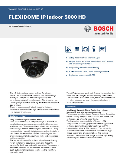
u1080p resolution for sharp imagesu Easy to install with auto zoom/focus lens, wizardand pre-configured modesu Fully configurable quad streamingu IR version with 15 m (50 ft) viewing distanceu Regions of interest and E-PTZThe HD indoor dome cameras from Bosch areprofessional surveillance cameras that provide highquality HD images for demanding security andsurveillance network requirements. These domes aretrue day/night cameras offering excellent performanceday or night.There is a version with a built-in active infraredilluminator that provides high performance in extremelow-light environments.System overviewEasy to install stylish indoor domeIdeal for indoor use, the stylish design is suitable forinstallations where appearance and flexible coverageare important. The varifocal lens allows you to choosethe coverage area to best suit your application. Usingthe proprietary pan/tilt/rotation mechanism, installerscan select the exact field of view. Mounting optionsare numerous, including surface, wall, and suspended-ceiling mounting.The automatic zoom/focus lens wizard makes it easyfor an installer to accurately zoom and focus thecamera for both day and night operation. The wizard isactivated from the PC or from the on-board camerapush button making it easy to choose the workflowthat suits best.The AVF (Automatic Varifocal) feature means that thezoom can be changed without opening the camera.The automatic motorized zoom/focus adjustment with1:1 pixel mapping ensures the camera is alwaysaccurately focused.FunctionsIntelligent Dynamic Noise Reduction reducesbandwidth and storage requirementsThe camera uses Intelligent Dynamic Noise Reductionwhich actively analyzes the contents of a scene andreduces noise artifacts accordingly.The low-noise image and the efficient H.264compression technology provide clear images whilereducing bandwidth and storage by up to 50%compared to other H.264 cameras. This results inreduced-bandwidth streams that still retain a highimage quality and smooth motion. The cameraprovides the most usable image possible by cleverlyoptimizing the detail-to-bandwidth ratio.Area-based encodingArea-based encoding is another feature which reduces bandwidth. Compression parameters for up to eight user-definable regions can be set. This allows uninteresting regions to be highly compressed, leaving more bandwidth for important parts of the scene. Bitrate optimized profileThe average typical optimized bandwidth in kbits/s for various image rates is shown in the table:Multiple streamsThe innovative multi-streaming feature delivers various H.264 streams together with an M‑JPEG stream. These streams facilitate bandwidth-efficient viewing and recording as well as integration with third-party video management systems.Depending on the resolution and frame rate selected for the first stream, the second stream provides a copy of the first stream or a lower resolution stream.The third stream uses the I-frames of the first stream for recording; the fourth stream shows a JPEG image at a maximum of 10 Mbit/s.Regions of interest and E-PTZRegions of Interest (ROI) can be user defined. The remote E-PTZ (Electronic Pan, Tilt and Zoom) controls allow you to select specific areas of the parent image. These regions produce separate streams for remote viewing and recording. These streams, together with the main stream, allow the operator to separately monitor the most interesting part of a scene while still retaining situational awareness.Built-in microphone, two-way audio and audio alarm The camera has a built-in microphone to allow operators to listen in on the monitored area. Two-way audio allows the operator to communicate with visitors or intruders via an external audio line input and output. Audio detection can be used to generate an alarm if needed.If required by local laws, the microphone can be permanently blocked via a secure license key. Tamper and motion detectionA wide range of configuration options is available for alarms signaling camera tampering. A built-in algorithm for detecting movement in the video can also be used for alarm signaling.Storage managementRecording management can be controlled by the Bosch Video Recording Manager (VRM) or the camera can use iSCSI targets directly without any recording software.Edge recordingThe MicroSD card slot supports up to 2 TB of storage capacity. A microSD card can be used for local alarm recording. Pre-alarm recording in RAM reduces recording bandwidth on the network, or — if microSD card recording is used — extends the effective life of the storage medium.Cloud-based servicesThe camera supports time-based or alarm-based JPEG posting to four different accounts. These accounts can address FTP servers or cloud-based storage facilities (for example, Dropbox). Video clips or JPEG images can also be exported to these accounts.Alarms can be set up to trigger an e-mail or SMS notification so you are always aware of abnormal events.Easy installationPower for the camera can be supplied via a Power-over-Ethernet compliant network cable connection. With this configuration, only a single cable connection is required to view, power, and control the camera. Using PoE makes installation easier and more cost-effective, as cameras do not require a local power source.The camera can also be supplied with power from+12 VDC power supplies.For trouble-free network cabling, the camera supports Auto-MDIX which allows the use of straight or cross-over cables.True day/night switchingThe camera incorporates mechanical filter technology for vivid daytime color and exceptional night-time imaging while maintaining sharp focus under all lighting conditions.Hybrid modeAn analog video output enables the camera to operate in hybrid mode. This mode provides simultaneous high resolution HD video streaming and an analog video output via an SMB connector. The hybrid functionality offers an easy migration path from legacy CCTV to a modern IP-based system.Access securityPassword protection with three levels and 802.1x authentication is supported. To secure Web browser access, use HTTPS with a SSL certificate stored in the camera.Complete viewing softwareThere are many ways to access the camera’s features: using a web browser, with the Bosch Video Management System, with the free-of-chargeBosch Video Client or Video Security Client, with the video security mobile app, or via third-party software. Video security appThe Bosch video security mobile app has been developed to enable Anywhere access to HD surveillance images allowing you to view live images from any location. The app is designed to give you complete control of all your cameras, from panning and tilting to zoom and focus functions. It’s like taking your control room with you.This app, together with the separately available Bosch transcoder, will allow you to fully utilize our dynamic transcoding features so you can play back images even over low-bandwidth connections.System integrationThe camera conforms to the ONVIF Profile S, ONVIF Profile Q and ONVIF Profile G specifications. Compliance with these standards guarantees interoperability between network video products regardless of manufacturer.Third-party integrators can easily access the internal feature set of the camera for integration into large projects. Visit the Bosch Integration Partner Program (IPP) website () for more information.HD standardsComplies with the SMPTE 274M-2008 Standard in:–Resolution: 1920x1080–Scan: Progressive–Color representation: complies with ITU-R BT.709–Aspect ratio: 16:9–Frame rate: 25 and 30 frames/sComplies with the SMPTE 296M-2001 Standard in:–Resolution: 1280x720–Scan: Progressive–Color representation: complies with ITU-R BT.709–Aspect ratio: 16:9–Frame rate: 25 and 30 frames/sInstallation/configuration notesDimensions mm (inch)Parts included•Camera•Screw kit•Installation documentation Technical specificationsSensitivity – (3200K, reflectivity 89%, F1.3, 30IRE)Ordering informationFLEXIDOME IP indoor 5000 HDProfessional IP dome camera for indoor HD surveillance. Varifocal 3 to 10 mm f1.3 lens; IDNR; day/ night; H.264 quad-streaming; cloud services; motion/ tamper/audio detection; microphone; 1080pOrder number NIN-51022-V3FLEXIDOME IP indoor 5000 IRProfessional IP dome camera for indoor HD surveillance. Varifocal 3 to 10 mm f1.3 lens; IDNR; day/ night; H.264 quad-streaming; cloud services; motion/ tamper/audio detection; microphone; 1080p; infrared Order number NII-51022-V3FLEXIDOME IP indoor 5000 HDProfessional IP dome camera for indoor HD surveillance. Automatic Varifocal 3 to 10 mm f1.3 lens; DC iris; IDNR; day/night; H.264 quad-streaming; cloud services; motion/tamper/audio detection; microphone; 1080pOrder number NIN-50022-A3FLEXIDOME IP indoor 5000 IRProfessional IP dome camera for indoor HD surveillance. Automatic Varifocal 3 to 10 mm f1.3 lens; DC iris; IDNR; day/night; H.264 quad-streaming; cloud services; motion/tamper/audio detection; microphone; 1080p; infraredOrder number NII-50022-A3AccessoriesNDA-LWMT-DOME Dome Wall MountSturdy wall L-shaped bracket for dome cameras Order number NDA-LWMT-DOMENDA-ADTVEZ-DOME Dome Adapter BracketAdapter bracket (used together with appropriate wall or pipe mount, or surface mount box)Order number NDA-ADTVEZ-DOMEVEZ-A2-WW Wall MountWall mount (Ø145/149 mm) for dome cameras (use together with appropriate dome adapter bracket); whiteOrder number VEZ-A2-WWVEZ-A2-PW Pipe MountPendant pipe mount (Ø145/149 mm) for dome cameras (use together with appropriate dome adapter bracket); whiteOrder number VEZ-A2-PWLTC 9213/01 Pole Mount AdapterFlexible pole mount adapter for camera mounts (use together with the appropriate wall mount bracket). Max. 9 kg (20 lb); 3 to 15 inch diameter pole; stainless steel strapsOrder number LTC 9213/01NDA-FMT-DOME In-ceiling mountIn-ceiling flush mounting kit for dome cameras(Ø157 mm)Order number NDA-FMT-DOMENDA-ADT4S-MINDOME 4S Surface Mount BoxSurface mount box (Ø145 mm / Ø5.71 in) for dome cameras (use together with the appropriate dome adapter bracket).Order number NDA-ADT4S-MINDOMEMonitor/DVR Cable SMB 0.3M0.3 m (1 ft) analog cable, SMB (female) to BNC (female) to connect camera to coaxial cableOrder number NBN-MCSMB-03MMonitor/DVR Cable SMB 3.0M3 m (9 ft) analog cable, SMB (female) to BNC (male) to connect camera to monitor or DVROrder number NBN-MCSMB-30MNPD-5001-POE Midspan PoE InjectorPower-over-Ethernet midspan injector for use with PoE enabled cameras; 15.4 W, 1-portOrder number NPD-5001-POENPD-5004-POE Midspan PoE InjectorPower-over-Ethernet midspan injectors for use with PoE enabled cameras; 15.4 W, 4-portsOrder number NPD-5004-POERepresented by:North America:Europe, Middle East, Africa:Asia-Pacific:China:Latin America and Caribbean:Bosch Security Systems, Inc. 130 Perinton Parkway Fairport, New York, 14450, USA Phone: +1 800 289 0096 Fax: +1 585 223 9180***********************.com Bosch Security Systems B.V.P.O. Box 800025617 BA Eindhoven, The NetherlandsPhone: + 31 40 2577 284Fax: +31 40 2577 330******************************Robert Bosch (SEA) Pte Ltd, SecuritySystems11 Bishan Street 21Singapore 573943Phone: +65 6571 2808Fax: +65 6571 2699*****************************Bosch (Shanghai) Security Systems Ltd.203 Building, No. 333 Fuquan RoadNorth IBPChangning District, Shanghai200335 ChinaPhone +86 21 22181111Fax: +86 21 22182398Robert Bosch Ltda Security Systems DivisionVia Anhanguera, Km 98CEP 13065-900Campinas, Sao Paulo, BrazilPhone: +55 19 2103 2860Fax: +55 19 2103 2862*****************************© Bosch Security Systems 2016 | Data subject to change without notice 188****8507|en,V9,01.Jun2016。


rendertargetbitmap 参数解释
以下是对RenderTargetBitmap参数的详细解释:
PixelsWidth和PixelsHeight:这两个参数用于指定渲染目标位图的宽度和高度,以像素为单位。
这些参数决定了位图的尺寸,进而影响渲染输出的效果。
DpiX和DpiY:这两个参数用于指定位图的每英寸点数(DPI),分别表示X轴和Y 轴方向上的分辨率。
DPI值越高,输出的图像质量越好,但同时也需要更多的存储空间和处理性能。
PixelFormat:这个参数用于指定像素的格式,即每个像素使用的颜色信息。
常见的像素格式包括RGB、ARGB、Gray等,不同的格式适用于不同的图像类型和应用场景。
RenderTargetBitmapFactory:这个参数是一个可选的工厂类,用于创建RenderTargetBitmap对象。
通过使用工厂类,您可以更加灵活地控制位图的创建过程,例如设置位图的资源管理器和渲染上下文等。
RenderTargetBitmapOptions:这个参数是一个可选的结构体,提供了对RenderTargetBitmap对象进行更细粒度控制的选项。
例如,您可以设置是否使用双缓冲技术来减少图像闪烁现象,或者设置是否保留图像的纵横比等。
通过合理设置这些参数,您可以控制渲染目标位图的输出效果,以满足您的具体需
求。
请注意,这些参数的具体含义和用法可能会根据您使用的编程语言和库而有所不同。

主题:resolution scale切片计算公式1. 介绍resolution scale切片计算公式的背景和概念在计算机图形学中,resolution scale是用来描述屏幕上每个像素对应的三维空间中多大区域的概念。
在3D游戏和动画中,通常会使用resolution scale来调整图像的清晰度和性能之间的平衡。
而在计算resolution scale时,需要使用到切片计算公式来进行精确的计算。
2. resolution scale切片计算公式的基本原理切片计算公式主要是根据游戏或动画引擎中的虚拟相机的参数以及屏幕分辨率来计算每个像素在三维空间中所代表的区域大小。
这样可以根据resolution scale的值来动态调整每个像素在屏幕上的显示效果,从而实现性能和视觉效果的平衡。
3. resolution scale切片计算公式的具体推导resolution scale的计算通常涉及到像素密度、屏幕分辨率以及相机的参数等多个因素。
一般而言,resolution scale的计算公式可以表示为:\[ RS = \frac{1}{\sqrt{w^{2} + h^{2}}} \]其中,RS表示resolution scale的值,w和h分别表示屏幕的宽度和高度。
4. resolution scale切片计算公式的应用通过resolution scale切片计算公式,我们可以根据实际的情况动态地调整每个像素所代表的空间区域大小,从而在不同的硬件设备上实现更好的性能和视觉效果。
这在移动设备、虚拟现实和增强现实等领域都有重要的应用意义。
5. 总结resolution scale切片计算公式是计算机图形学中一个重要的概念,它在调整图像清晰度和性能平衡上具有重要作用。
通过合理地应用resolution scale切片计算公式,可以在不同的硬件评台上实现更好的视觉效果和性能表现。
希望未来可以有更多的研究和实践在这一领域取得突破,为计算机图形学的发展做出更大的贡献。

ubuant调整分辨率指令-回复ubuant调整分辨率指令是一种用于调整计算机显示屏分辨率的命令。
分辨率是指屏幕上显示的像素数量,通常以水平像素数乘以垂直像素数来表示。
调整分辨率可以改变屏幕上显示的图像的清晰度和细节,对于不同的应用场景和个人需求,选择合适的分辨率非常重要。
本文将一步一步解析ubuant调整分辨率指令的用法和作用,帮助读者了解如何有效地调整分辨率。
首先,我们需要明确ubuant调整分辨率指令的具体形式和可用参数。
在ubuant系统中,我们可以使用xrandr命令来调整分辨率。
它是一个功能强大的命令行工具,用于配置和管理显示设备和显示器的分辨率、刷新率和方向等参数。
要使用ubuant调整分辨率指令,我们首先需要打开终端。
在ubuant系统中,按下Ctrl + Alt + T快捷键可以快速打开终端。
接下来,输入以下命令,然后按下Enter键以执行该命令:xrandr这将显示当前系统中所有连接的显示屏和可用的显示模式。
每个显示屏和显示模式都有一个唯一的标识符,我们将使用这些标识符来选择和调整分辨率。
注意,如果您的系统中只有一个显示屏,则窗口上没有其他内容显示。
接下来,我们需要确定当前显示模式的名称。
执行以下命令,然后按下Enter键:xrandr verbose这将显示关于当前显示模式的更多详细信息,包括名称、分辨率和刷新率等。
请注意屏幕名称,因为我们将在下一步中使用它。
现在,我们可以开始调整分辨率。
执行以下命令,然后按下Enter键:xrandr output <屏幕名称> mode <分辨率>将“<屏幕名称>”替换为您在上一步中确定的屏幕名称,并将“<分辨率>”替换为您希望设置的分辨率。
例如,如果您的屏幕名称为“LVDS-1”且您希望将分辨率设置为“1920x1080”,则命令应如下所示:xrandr output LVDS-1 mode 1920x1080执行该命令后,您的屏幕将立即应用新的分辨率。

常用类1.VirtualUniverse类、Locale类与HiResCoord类之间的关系Virtual Universe 包含Locale 包含BranchGroup每一个Locale对象都具有一个高分辨率大尺度坐标系,每一个Locale对象的高分辨率大尺度坐标系都用3个高分辨率大尺度数来定义其原点的坐标值x,y,z (用HiResCoord类定义)。
VirtualUniverse类定义的对象是包含所有场景图的最高级别的容器。
2.SimpleUniverse类该类可快速地设置一个最小的用户环境,并且很容易使一个Java3D应用程序运行起来。
该实用程序类创建了场景图中与观察相关的所有必须对象。
该类创建了一个Locale, 一个单独的ViewingPlatform和一个Viewer观察者对象。
但此类不适合复杂应用程序。
SimpleUniverse 包含Locale 包含BranchGroup 包含TransformGroup 包含ViewPlatform3.Bounds类用于限定特定操作的作用范围用于确定某种动作或行为的范围。
用于确定某种全景操作的应用范围4.SharedGroup类共享子图。
SharedGroup节点作为共享子图的根节点。
Link叶子节点链接向该SharedGroup节点,并不是将共享子图集成到当前场景图中。
一个SharedGroup 节点允许多个Link叶子节点同时通过链接的方式共享该子图。
5.View类观察模型。
应用Java3D观察模型编写的应用程序在不修改场景图的情况下,能够将可视化后的图像显示到各种不同的显示设备上“一次编写到处运行”6.ViewPlatform类在虚拟世界中的观察平台。
一个ViewPlatform叶子节点在虚拟世界中定义了一个坐标系和一个具有相关原点或参考点的参考框架。
ViewPlatform作为观察对象的依附点,并且其作为一个可视化器观察的基点。
7.ViewingPlatform类Java3D的三种坐标系:世界坐标系,观察坐标系,显示器坐标系透视投影:当给定视点、观察方向与投影平面后,将世界坐标系转换为观察坐标系,对观察坐标系中的三维物体通过比例变换向投影平面投影。

qgraphicssimpletextitem 清空文本-回复如何清空文本?清空文本是在编程中经常遇到的操作之一。
在Qt框架中,可以利用QGraphicsSimpleTextItem类来创建和操作文本对象。
本文将详细介绍如何使用QGraphicsSimpleTextItem类清空文本内容。
首先,我们需要创建一个QGraphicsScene对象来承载我们的文本对象。
在Qt中,QGraphicsScene用于管理和协调场景中的所有图形项。
我们可以使用以下代码来创建一个QGraphicsScene对象:cppQGraphicsScene *scene = new QGraphicsScene();接下来,我们需要创建一个QGraphicsSimpleTextItem对象。
在创建对象时,我们可以指定文本内容、字体、字号、颜色等属性。
使用以下代码来创建一个QGraphicsSimpleTextItem对象:cppQGraphicsSimpleTextItem *textItem = new QGraphicsSimpleTextItem("这是一个文本对象");textItem->setFont(QFont("Arial", 12));textItem->setBrush(Qt::black);在创建文本对象后,我们可以将它添加到场景中。
使用以下代码将文本对象添加到场景中:cppscene->addItem(textItem);此时,文本对象已经显示在场景中。
接下来,我们需要编写一个函数来清空文本内容。
可以使用以下代码来清空文本内容:cppvoid clearText(QGraphicsSimpleTextItem *textItem) {textItem->setText("");}在上述函数中,我们通过调用setText("")函数将文本内容设置为空字符串,即可实现文本内容的清空。


Mental ray 下Render Global Settings的参数属性Quality Presets 是Mental ray渲染质量的事先调整Min sample level Max sample level是Mental ray渲染时设定一个像素最少和最大的取样次数。
May是采用连续的整数,而Mental ray采用指数:2的2乘以min samples 次方。
如果min sample level 是0,那么基本采样时1次。
通常Max sample level取-2,-1,0,1。
最大采样相当于1/16,1/4,1,4。
通常Max sample level取0,1,2,3。
最大采样相当于1,4,16,256。
min samples和Max sample level之间的差值是细化的程度限制。
差值一般不要超过3。
Filter 过滤不要将filter的像素过滤值调节到小于默认的值Box 简单的,对周围像素平均对待的方式仅向周围上下左右各扩展一个像素。
Triangle是一种对周围像素用随着距离直线下降的比例的比例对待方式。
Gauss 对周围像素的采用比例曲线是先缓慢下降,然后急速下降,最后缓慢下降到0。
Mitchell,Lanczos 等同于Gauss,默认值为4,使图像的变化更平滑,保持好的图像比例。
Contrast Threhol 对比度是相邻采样区域之间的颜色对比,如果这个对比大,则认为图像存在突然变化,与就是锯齿,需要细化。
May提供的默认的红,绿,蓝三色的对比度是值得参考的。
0.2:0.15:0.3。
我们设置的比例可按照这个比例!当对比值小于0.05时,通常只会增缴渲染时间,而对效果不会有任何的提高。
当我们将min samples和Max sample level设置为一样时,那么我们就是取消了细化取样,使得对比值失效。
同时对比值都设为1,会使最大取样失效。
想得到好的画面质量,min samples和Max sample level,Contrast Threhol都不可忽视。

Key FeaturesThe 3440x1440 resolution is 2.5 times than Full HD, providing much more detailed graphics More space to spread out your various work windows for more productive multitasking provides brighter imagery and supports the cinema-standard 98% DCI-P3 color gamutUp to 120 Hz Variable Refresh Rate with FreeSync Premium Pro to optimize fast-rendering scenario*Factory pre-calibrated with ASUS advanced gray-scale tracking technology to guarantee the △E color difference value is less than 2USB-C connection for DisplayPort, USB data transmission and supports 90W power deliveryUp to 400 nits brightness with HDR for lifelike contrast & color that brings out details like never before A convenient mounting clamp is included to help free up desk space*Ergonomically-designed stand with tilt, swivel, pivot, and heightadjustmentsHigh Refresh Rate *FreeSync Premium Pro up to 120 Hz for DisplayPort and USB-C, Adaptive-Sync up to 100Hz for HDMI.*Desk C-clamp availability may vary by region.Display Panel Size : 34-inch (86.36cm) Wide Screen (21:9) Display Viewing Area(HxV) : 799.8 x 334.8 mm Display Surface : Non-Glare Panel Type : IPS Viewing Angle (CR ≧10, H/V) : 178°/ 178°Pixel Pitch : 0.2325 mm Resolution : 3440x1440Color Space (sRGB) : 100%Color Space (Rec. 709) : 100%Color Space (DCI-P3) : 98%Brightness (HDR, Peak) : 400 cd/㎡/ (Typ.) : 350cd/㎡Contrast Ratio (Typ.) : 1000:1Display Colors : 1073.7M (10 bit)Response Time : 2ms (GTG)Refresh Rate (Max) : 120Hz (for DisplayPort and USB-C ports)HDR (High Dynamic Range) Support : HDR-10Flicker-free : YesVideo Feature Trace Free Technology : Yes ProArt Preset : Standard / sRGB / Rec. 709 / DCI-P3 / HDR / Scenery / Reading / Rapid Rendering / User Mode 1 / User Mode 2Color Temp. Selection : Yes (5 modes)Color Adjustment : 6-axis adjustment (R,G,B,C,M,Y)Gamma adjustment : Yes (Support Gamma 1.8/2.0/2.2/2.4/2.6 )Color Accuracy : △E< 2ProArt Palette : Yes QuickFit Plus : Yes PIP / PBP Technology : Yes HDCP : Yes, 2.2VRR Technology : FreeSync ™Premium Pro (for DisplayPort and USB-C ports)ProArt Chroma Tune : Yes Low Blue Light : YesAudio Feature Speaker : Yes (2Wx2)IO portsUSB-C x 1DisplayPort 1.4 x 1HDMI(v2.0) x 2USB Hub : Yes (USB 3.2 Gen 1 Type-A x 4)Earphone Jack : Yes Power Delivery : 90W Signal FrequencyDigital Signal Frequency : HDMI: 30~151 KHz (H) / 30~100 Hz (V)USB-C, DisplayPort: 185~185 KHz (H) / 48~120 Hz (V)PowerConsumptionPower On (Typical): < 19.36W Power Saving Mode : < 0.5W ; Power Off Mode : 0W (Hard Switch)100-240V, 50/60Hz Mechanical DesignTilt : Yes (+23°~ -5°)Swivel : Yes (+30°~ -30°)Height Adjustment : 0~115mm VESA Wall Mounting : 100x100mm Kensington Lock : Yes Dimensions (Est.)Phys. Dimension with Stand (W x H x D) : 817.6 x (453.9~568.9) x 245 mm Phys. Dimension without Stand (W x H x D) : 817.6 x 368.2 x 68.9 mm Box Dimension (W x H x D) : 930 x 488 x 300 mm Weight(Est.)Net Weight with Stand : 12.2 kg Net Weight without Stand : 7.8 kg Gross Weight : 17 kg (WW)/ 15.7 kg (NA)AccessoriesPower cord,USB-C cable (optional), HDMI cable (optional), DisplayPort cable (optional), Calibration Report, Quick Start Guide, Warranty Card, Welcome Card, Desk C-clamp (optional)ComplianceStandard FCC, UL/cUL, ICES-3, CB, CE, ErP, WEEE, TUV-GS, TUV-Ergo, ISO 9241-307, UkrSEPRO, CU, CCC, CEL, BSMI, RCM, AU MEPS, VCCI, PSE, J-MOSS, KC, KCC, e-Standby, PSB, BIS, VN MEPS, Energy Star, TCO, RoHS, CEC, TÜV Flicker Free, TÜV Low Blue Light, VESA DisplayHDR 400, AMD FreeSync PremiumPro, VESA MediaSync* Power Consumption is measuring a screen brightness of 200 nits without audio / USB / Card reader connection **All specifications are subject to change without notice Spec SheetDisplayPort1.4HDMI (v2.0) x 2Earphone Jack USB Hub Full Function USB-C。
QSplat:A Multiresolution Point Rendering System for Large MeshesSzymon RusinkiewiczMarc LevoyStanford UniversityAbstractAdvances in3D scanning technologies have enabled the practical cre-ation of meshes with hundreds of millions of polygons.T raditional algorithms for display,simplification,and progressive transmission of meshes are impractical for data sets of this size.We describe a system for representing and progressively displaying these meshes that com-bines a multiresolution hierarchy based on bounding spheres with a rendering system based on points.A single data structure is used for view frustum culling,backface culling,level-of-detail selection, and rendering.The representation is compact and can be computed quickly,making it suitable for large data sets.Our implementa-tion,written for use in a large-scale3D digitization project,launches quickly,maintains a user-settable interactive frame rate regardless of object complexity or camera position,yields reasonable image qual-ity during motion,and refines progressively when idle to a highfinal image quality.We have demonstrated the system on scanned models containing hundreds of millions of samples.Categories and Subject Descriptors:I.3.3[Computer Graphics]: Picture/Image Generation–Display Algorithms;I.3.5[Computer Graphics]:Computational Geometry and Object Modeling–Curve, surface,solid,and object representations;I.3.6[Computer Graph-ics]:Methodology and T echniques–Graphics data structures and data types.Keywords:Rendering systems,Spatial data structures,Level of detail algorithms,Compression algorithms1IntroductionA significant recent trend in computer graphics has been the shift to-wards using sampled representations of real objects during rendering. An example of this trend has been the increased use of3D scanning systems,which produce three-dimensional sampled models of phys-ical objects.One problem with3D scanners,however,is handling Stanford Computer Graphics LabGates Building3BStanford UniversityStanford,CA94305{smr,levoy}@ the large amounts of data they produce.Over the past several years, improvements in the hardware and software components of3D scan-ning systems have increased the practically attainable sizes of scanned meshes to hundreds of millions of samples.Current workstations can not display meshes of this size in real time,and the running time and space requirements of traditional mesh simplification and progressive display algorithms make these approaches impractical for scanned meshes containing more than a few million samples.Moreover,many such techniques focus on op-timizing the placement of individual edges and vertices,expending a relatively large amount of effort per vertex.Scanned data,however, has a large number of vertices and their locations are often impre-cise due to noise.This suggests an alternative approach in which individual points are treated as relatively unimportant,and conse-quently less effort is spent per primitive.Recent research employing this paradigm includes the spline-fitting system by Krishnamurthy and Levoy[Krishnamurthy96],the range image merging system by Cur-less and Levoy[Curless96],and Yemez and Schmitt’s rendering sys-tem based on octree particles[Yemez99].These algorithms do not treat range data as exact,and in fact do not preserve the3D locations of any samples of the original mesh.Following this trend of algorithms with low per-primitive cost,we have developed a new algorithm for interactive display of large meshes. The implementation,dubbed QSplat,was designed during the course of a large3D digitization project[Levoy00].Because it uses a simple rendering algorithm based on traversing a bounding sphere hierarchy, it is suitable for browsing the models generated during this project, which contain100million to1billion samples.Additionally,QSplat does not maintain the connectivity of the input mesh(which in the case of scanned data inherently is only useful to resolve depth disconti-nuities and has little other meaning),instead relying on a point-based representation and splat rendering.As a result,our system has lower preprocessing and rendering costs than comparable polygon-based sys-tems.QSplat launches quickly,adjusts level of detail to maintain an interactive frame rate,and has a compact in-memory and on-disk rep-resentation.In this paper,we present the QSplat data structure and rendering algorithm and discuss some of the tradeoffs and design decisions in-volved in making it practical for large meshes.We describe the ren-dering performance of the system,and discuss its preprocessing costs. Finally,we consider its relation to previous algorithms for displaying large meshes,and describe some future extensions for rendering other kinds of large geometric data sets.2QSplat Data Structure and Algorithms QSplat uses a hierarchy of bounding spheres[Rubin80,Arvo89]for visibility culling,level-of-detail control,and rendering.Each node of the tree contains the sphere center and radius,a normal,the width of a normal cone[Shirman93],and optionally a color.One couldPermission to make digital or hard copies of part or all of this work or personal or classroom use is granted without fee provided that copies are not made or distributed for profit or commercial advantage and that copies bear this notice and the full citation on the first page. To copy otherwise, to republish, to post on servers, or to redistribute to lists, requires prior specific permission and/or a fee.SIGGRAPH 2000, New Orleans, LA USA© ACM 2000 1-58113-208-5/00/07 ...$5.00generate such a bounding sphere hierarchy from polygons,voxels,or point clouds,though for our application we only needed an algorithm for generating the hierarchy from triangular meshes.The hierarchy is constructed as a preprocess,and is written to disk.2.1Rendering AlgorithmOnce the hierarchy has been constructed,the following algorithm is used for display:T raverseHierarchy(node){if(node not visible)skip this branch of the treeelse if(node is a leaf node)draw a splatelse if(benefit of recursing further is too low)draw a splatelsefor each child in children(node)T raverseHierarchy(child)}We now examine several stages of this basic algorithm in detail. Visibility Culling:As we recurse the bounding sphere hierarchy,we cull nodes that are not visible.Frustum culling is performed by testing each sphere against the planes of the view frustum.If the sphere lies outside,it and its subtree are discarded and not processed further.If the sphere lies entirely inside the frustum,this fact is noted and no further frustum culling is attempted on the children of the node. We also perform backface culling during rendering,using the nor-mal and cone of normals stored at each node.If the cone faces entirely away from the viewer,the node and its subtree are discarded.We also detect the case of a cone pointing entirely towards the viewer,and mark its children as not candidates for backface culling. Determining When to Recurse:The heuristic used by QSplat to decide how far to recurse is based on projected size on the screen.That is,a node is subdivided if the area of the sphere,projected onto the viewing plane,exceeds a threshold.The cutoffis adjusted from frame to frame to maintain a user-selected frame rate.We currently use a simple feedback scheme that adjusts the threshold area by the ratio of actual to desired rendering time on the previous frame.Funkhouser and Séquin have demonstrated a predictive algorithm for LOD con-trol that results in smaller frame-to-frame variation of rendering times [Funkhouser93];however,we have not implemented this.We also have not incorporated any algorithm for smooth transitions as sections of the model change from one level of detail to another,such as the geomorphs in Hoppe’s progressive mesh system[Hoppe98].Given the modest changes in appearance as we refine and the quick changes in viewpoint typical in our application,we have not found the absence of smoothing visually significant;other applications,however,might benefit from smoother transitions.Although screen-space area is the most popular metric for LOD control,other heuristics have been proposed for determining how far to recurse[Duchaineau97,Hoppe97].Within the framework of our system,one could incorporate rules for recursing further around sil-houette edges(using per-node normals),in areas of high curvature (using normal cone widths),or in the central“foveal”region of the screen(which uses only projected position).The above implementation of frame rate control is used during in-teractive manipulation of the model.Once the user stops moving the mouse,we redraw the scene with successively smaller thresholds until a size of one pixel is reached.Figure1shows a sample scene rendered by QSplat at several levels of refinement.Drawing Splats:Once we have either reached a leaf node or de-cided to stop recursing,we draw a splat representing the current sphere [Westover89].The size of the splat is based on the projected diameter of the current sphere,and its color is obtained from a lighting calcu-lation based on the current per-sphere normal and color.Splats are drawn with Z-buffering enabled to resolve occlusion.We discuss the shape of each splat in Section3.3.2.2Preprocessing AlgorithmOur preprocessing algorithm begins with a triangular mesh represent-ing the model to be encoded.Although one could build up a QSplat hierarchy directly from a point cloud,starting with a mesh makes it easy to compute the normals at each node.If we did not have a mesh, we would have to compute normals byfitting a plane to the vertices in a small neighborhood around each point.Beginning with a mesh also makes it possible to assign sphere sizes to the input vertices(which become the leaf nodes in our bounding sphere hierarchy)such that no holes are left during rendering.In order to guarantee this,the sizes must be chosen such that if two vertices are connected by an edge of the original mesh,the spheres placed at those vertices are large enough to touch.Our current algorithm makes the size of the sphere at a ver-tex equal to the maximum size of the bounding spheres of all triangles that touch that vertex.This is a conservative method–it may result in spheres that are too large,but is guaranteed not to leave any holes. Once we have assigned leaf sphere sizes,we use the following algo-rithm to build up the rest of the tree:BuildT ree(vertices[begin..end]){if(begin==end)return Sphere(vertices[begin])elsemidpoint=PartitionAlongLongestAxis(vertices[begin..end])leftsubtree=BuildT ree(vertices[begin..midpoint])rightsubtree=BuildT ree(vertices[midpoint+1..end])return BoundingSphere(leftsubtree,rightsubtree)}The algorithm builds up the tree by splitting the set of vertices along the longest axis of its bounding box,recursively computing the two subtrees,andfinding the bounding sphere of the two children spheres.As the tree is built up,per-vertex properties(such as normal and color)at interior nodes are set to the average of these properties in the subtrees.When the recursion reaches a single vertex,we simply create a sphere whose center is the position of the vertex.Because the total size of a tree depends on the branching factor at each node,we combine nodes in the tree to increase the average branching factor to approximately4.This reduces the number of interior nodes,thereby reducing the storage requirements for the tree.Thefinal step of pre-processing is quantizing all of the properties at each node,as described in Section3.1.3Design Decisions and TradeoffsLet us now consider some of the decisions made in the implementa-tion of QSplat that make it suitable for our application of visualizing large scanned data sets.We describe how tradeoffs in quantization,file layout,splat shape,and the choice of splatting were affected by our goals of fast rendering and compact representation.15-pixel cutoff130,712points132ms10-pixel cutoff259,975points215ms5-pixel cutoff1,017,149points722ms1-pixel cutoff14,835,967points8308msFigure1:A model of Michelangelo’s statue of St.Matthew rendered by QSplat at several levels of refinement.Rendering was done on an SGI Onyx2with InfiniteReality graphics,at a screen resolution of1280x1024.The model was generated from a mesh with127million samples,representing a statue2.7meters tall at0.25mm resolution.The images at right are closeups of the outlined areas at left.3 bits 16 bits2 bits 14 bits13 bits Figure 2:QSplat file and node layout.(a)The tree is stored in breadth-first order (i.e.,the order given by the red arrows).(b)The link from parent to child nodes is established by a single pointer from a group of parents to the first child.The pointer is not present if all of the “parent”siblings are leaf nodes.All pointers are 32bits.(c)A single quantized node occupies 48bits (32without color).3.1Node Layout and QuantizationThe layout of each node in the bounding sphere hierarchy is shown in Figure 2c.A node contains the location and size of a sphere relative to its parent,a normal,the width of a cone of normals,an optional color,and a few bits used in representing the structure of the tree.We discuss the structure of the tree and the layout of nodes within the file in Section 3.2.Position and radius:The position and radius of each sphere is en-coded relative to its parent in the bounding sphere hierarchy.In order to save space,these quantities are quantized to 13values.That is,the radius of a sphere can range from 113to 1313of the radius of its par-ent,and the o ffset of the center of a sphere relative to the center of its parent (in each of X,Y,and Z)is some multiple of 113of the di-ameter of the parent sphere.The quantization proceeds top-down,so the position and size of a child sphere is encoded relative to the quan-tized position of its parent;thus,quantization error does not propagate down the mesh.In order to guarantee that the quantization process does not introduce any holes,the quantized radius is always rounded up to the nearest representable value that ensures that the quantized sphere completely encloses the true sphere.Note that not all of the 134possible combinations of x ,y ,z center o ffset and radius ratio are valid,since many result in child spheres that are not enclosed by their parents.In fact,only 7621of the possible combinations are valid,which means that we can encode the quan-tized position and radius using only 13bits (using a lookup table).For a parent sphere of radius 1,this encoding scheme gives a mean quantization error of 0.04in the x ,y ,and z components of a child sphere,and a mean error of 0.15in the child sphere’s radius.The er-ror in the radius is larger than the error in position because the radius is first increased by the quantization error in the position of the sphere (to ensure that the quantized sphere encloses the true sphere),and is then always rounded up to the next representable value.We could ob-tain lower quantization error in the radius by not insisting that the quantized sphere completely enclose the original.Doing so,how-ever,would introduce the possibility that spheres that should touch no longer do so after the quantization.This could produce holes in our renderings.The idea of representing geometric quantities such as sphere po-sitions by encoding them incrementally,thereby essentially spreading out the bits of the quantities among the levels in the hierarchy,rep-resents a departure from traditional approaches to mesh compression,which rely on encoding the di fferences between vertex positions along some path along the edges of the mesh [Taubin 98].This “hierarchical delta coding”is,in fact,closer to the wavelet representation of geom-etry used in the multiresolution analysis of Eck et.al.[Eck 95].Our space requirement of 13bits per node appears competitive with state-of-the-art geometric compression methods,which average 9-15bits per vertex depending on initial quantization of vertex positions.This is not an entirely valid comparison,however,since traditional geomet-ric compression methods also represent mesh connectivity (which we discard),and since our 13bits per node also includes sphere radius.The position and radius of each node are decoded on-the-fly during rendering.Because of this,our data structure is not only compact on disk,but also requires less memory during rendering than methods that must decompress their data before rendering.Normals:The normal at each node is stored quantized to 14bits.The representable normals correspond to points on a 5252grid on each of the 6faces of a cube,warped to sample normal space more uniformly.A lookup table is used during rendering do decode the rep-resentable normals.In practice the use of only 52526=16224dif-ferent normals (leading to a mean quantization error of approximately 0.01radian)produces no visible artifacts in the di ffuse shading com-ponent,but some banding artifacts are visible around specular high-lights in broad areas of low curvature.It would be possible to eliminate these artifacts,as well as achieve better compression,by moving to an incremental encoding of each normal relative to the normal of the parent sphere.This would,however,increase the computational com-plexity of the inner loop of the algorithm,resulting in a time-space tradeo ff.Unlike the range of node positions,the space of normals is bounded,so a fixed quantization table su ffices for encoding the nor-mals of arbitrary scenes.Therefore,at this time we have chosen to use a fixed quantization for the normals,which requires only a single table lookup at run time.As processor speed increases,we anticipate that the incremental quantization scheme will become more attractive.Colors:Colors are currently stored quantized5-6-5to16bits.As in the case of normals,an incremental encoding of colors would save space but be more expensive at run time.Normal cones:After some experimentation,we have decided to quantize the width of the cone of normals at each node to just2bits. The four representable values correspond to cones whose half-angles have sines of116,416,916,and1616.On typical data sets,backface culling with these quantized normal cones discards over90percent of nodes that would be culled using exact normal cone widths.Note that we are always conservative in representing normal cone widths,so we never discard geometry that should be displayed.As with normals and colors,the normal cone widths could be represented relative to the widths at the parent nodes,but this would slow down rendering. 3.2File Layout and PointersThe nodes of the bounding sphere hierarchy are laid out(both in memory and on disk)in breadth-first order.A primary consequence of this is that thefirst part of thefile contains the entire mesh at low resolution.Thus,we only need to read in thefirst part of a file in order to visualize the model at low resolution;we see greater detail as more of thefile is read in from disk.We currently use OS-provided memory mapping as the basis for working-set management, so high-resolution data for a given section of the model is read in from disk when the user looks at it.This progressive loading is im-portant for usability with large models,for which the time to load the entire data set from disk may be several minutes.Because data is loaded as it is needed,rendering performance will be lower the first time the user zooms in on some area of the model–due to our feedback-based approach to frame rate control,there is a glitch in the frame rate.Subsequent frames that touch the same area of the model,however,are rendered at full speed.Speculative prefetching has been explored as a method for reducing this performance varia-tion[Funkhouser92,Funkhouser96,Aliaga99],but we currently do not implement this.Several pointerless schemes have been proposed for tree encod-ing,including linear octrees and methods based on complete trees [Samet90].These data structures,however,are inappropriate for our application.Linear octrees and related ideas require the entire tree to be traversed to recover its structure,which is impractical in our sys-tem.Data structures based on complete trees can be used for partial traversals,but because the algorithm we use to generate our trees is based on axis-aligned bisections,we can not guarantee that the result-ing trees will be complete and balanced.Furthermore,modifying the preprocessing algorithm to generate complete trees would not be de-sirable,since putting an equal number of vertices in each subtree can potentially put the splitting planes significantly off-center.Given the amount of quantization we perform on child sphere centers,this could lead to significant inaccuracies in the compressed tree.Although we can not use pointerless encodings for our trees,we should at least attempt to minimize the number of pointers required. Given that we store the tree in breadth-first order,it is sufficient to have one pointer for each group of siblings in the tree(i.e.children of a single parent sphere),that points to the children of these nodes. Furthermore,that pointer is not necessary if none of these spheres have children(i.e.they are all leaf nodes).Using this scheme,approx-imately8to10percent of the total storage cost is devoted to pointers, which we judged to be sufficiently small that we did not pursue more complicated schemes for reducing pointer costs further.In order to be able to traverse the tree,we store at each node two bits encoding the number of children of the node(0,2,3,or4children–nodes with a single child are not permitted),and one bit indicating whether all children of this node are leaf nodes.The total storage requirements for a tree may now be computed as the number of nodes in the tree multiplied by the cost per node, plus the overhead due to pointers.For a tree with average branching factor3.5,the total number of nodes will be1.4times the number of leaf nodes,making the net storage requirements for the entire tree approximately9bytes times the number of leaf nodes,or6bytes if colors are not stored.3.3Splat ShapeThe choice of kernel used to represent a rendered point sample can have a significant effect on the quality of thefinal image.The sim-plest,fastest option is a non-antialiased OpenGL point,which is ren-dered as a square.A second choice is an opaque circle,which may be rendered as a group of small triangles or,less expensively in most OpenGL implementations,as a single texture-mapped polygon.An-other possibility is a fuzzy spot,with an alpha that falls offradially with a Gaussian or some approximation.The particular approximation we use is a spline in opacity that falls to12at the nominal radius of the splat.These last two options will be slower to draw,since they require sending more data to the graphics pipeline.In addition,drawing a Gaussian splat requires special care regarding the order in which the splats are drawn,because of the interaction between blending and Z-buffering.Levoy and Whitted discuss this problem in the context of a software-only renderer[Levoy85];they propose an approach based on buckets to ensure that both occlusion and blending happen correctly. In OpenGL we can use multipass rendering to implement the correct behavior.For thefirst pass,depth is offset away from the viewer by some amount z,and we render only into the depth buffer.For the second pass we turn offdepth offset and render additively into the color buffer,with depth comparison but not depth update enabled. This has the effect of blending together all splats within a depth range zof the surface,while maintaining correct occlusion.Figure3com-pares these three choices of splat kernel.Because per-splat drawing time on current hardware is different for each kernel,we present com-parisons at both constant splat size and constant running time. Another option we have in choosing splat shape is the choice of whether the splats are always round(or square in the case of OpenGL points)or elliptical.In the latter case,the normal at each node is used to determine the eccentricity and orientation of the ellipse.When the normals point towards the viewer,the splats will be circular.Other-wise,the minor axis of each ellipse will point along the projection of the normal onto the viewing plane,and the ratio of minor to major axes will equal n v,where n is the normal of the splat and v is a vector pointing towards the viewer.This improves the quality of silhouette edges compared to circular splats,reducing noise and thickening.We compare the use of circular and elliptical splats in Figure4. Because we construct our bounding sphere hierarchy such that spheres placed along a continuous surface will never leave holes,we can guarantee that the square and circular kernels will always result in hole-free reconstructions.Our approximation to a Gaussian kernel is also guaranteed to produce full opacity in areas that started out as continuous surfaces.When we move to elliptical kernels,we can no longer guarantee hole-free reconstructions because normals need not be continuous along the surface.In practice,we do occasionally see holes when using elliptical kernels,especially around silhouette edges. We have found that restricting the maximum foreshortening of ellipses (e.g.clamping the maximum ratio of major to minor axis to10)fills in practically all of these holes.3.4Consequences of a Point-Based SystemThe fact that QSplat uses points as its rendering primitives makes it most suitable for certain kinds of scenes.In particular,point render-Figure 3:Choices for splat shape.We show a scene rendered using squares,circles,and Gaussians as splat kernels.In the top row,each image uses the same recursion threshold of 20pixels.Relative to squares,circles take roughly twice as long to render,and Gaussians take approximately four times as long.The Gaussians,however,exhibit significantly less aliasing.In the bottom row,the threshold for each image is adjusted to produce the same rendering time in each case.According to this criterion,the square kernels appear to o ffer the highest quality.Figure 4:Circular vs.elliptical splats.In the left image,all splats are circular with diameter 20pixels.In the right image,we draw elliptical splats rotated and foreshortened depending on per-node normals.This reduces thickening and noise around silhouette edges.Recursion depth has deliberately been limited to make the splats large enough to see in this visualization.(a)(b)(c)PointsPolygons –same number of primitives as (a)Polygons –same number of vertices as (a)Same rendering time as (a)T wice the rendering time of (a)Figure 5:Comparison of renderings using point and polygon primitives.ing systems are most e ffective for objects with uniformly-sized geo-metric detail,and in applications where it is not necessary to look at the model at significantly higher resolution than the spacing between samples.If the model has large,flat or subtly curved surfaces,polyg-onal models can be more compact and faster to draw.Similarly,if it is necessary to zoom in such that the spacing of samples is large com-pared to pixel size,polygons o ffer higher visual quality,especially near sharp edges and corners.Figure 5shows a comparison between point-and polygon-based renderings.QSplat was developed with the intent of visualizing scanned mod-els that contained significant amounts of fine detail at scales near the scanning resolution.We used the Volumetric Range Image Processing (VRIP)system [Curless 96]to merge raw scans into our final mod-els,and the marching cubes algorithm [Cline 88]to extract a polyg-onal mesh.Since the latter produces samples with a uniform spac-ing,point rendering was well-suited for our application domain.For scenes with large,smooth regions,we expect that QSplat would be less e ffective relative to polygon-based systems.The visual quality of the resulting models would still be good,however,if the large polygons were diced,as in the REYES architecture [Cook 87].For applications containing both high-frequency detail and large flat regions,hybrid point/polygon schemes might be appropriate.4PerformanceAs described in Section 3,the goal of interactivity dictated many de-sign decisions for our system.In addition to these,we have optimized our implementation in several ways in order to increase the size of the models we can visualize.4.1Rendering PerformanceThe majority of rendering time in our system is spent in an inner loop that traverses the hierarchy,computes the position and radius of each node,performs visibility culling,and decides whether to draw a point or recurse further.This inner loop was tuned to eliminate expensive operations,especially at lower levels of the tree.For example,we do not perform an exact perspective divide at the low levels of the tree,switching to an approximation when the screen-space size of a node reaches a few pixels.As a result,on average our algorithm can render between 1.5and 2.5million points per second on an SGI Onyx2once data has been read in from disk.The exact rate varies depending on caching e ffects (for example,we observe a speedup when the workingset fits in L2cache)and how much data is culled at which levels in the tree.Our display rate may be compared to the 480thousand polygons per second (on identical hardware)reported by Hoppe for his im-plementation of progressive meshes [Hoppe 98]or the 180thousand polygons per second for the ROAM system [Duchaineau 97].For our application,we typically use frame rates of 5-10Hz,meaning that we draw 200to 300thousand points per frame during interactive ren-dering.Note that unlike the above two systems,QSplat makes no explicit use of frame-to-frame coherence,such as cached lists of prim-itives likely to be visible.QSplat’s rendering performance is summa-rized in Figure 6.The simplicity of our algorithm makes it well suited for implemen-tation on low-end machines.As an extreme example,we have imple-mented QSplat on a laptop computer with no 3D graphics hardware (366MHz Intel Pentium II processor,128MB memory).Because rendering is performed in software,the system is fill limited.For a typical window size of 500x500and frame rate of 5Hz,the imple-mentation can traverse 250to 400thousand points per second,has a 40million pixel per second fill rate,and typically draws 50to 70thou-sand splats per frame.At this resolution the implementation is still comfortably usable.Although most present desktop systems do have 3D graphics hardware,the same is not true for portable and handheld systems,and in applications such as digital television set-top boxes.We believe that QSplat might be well-suited for such environments.4.2Preprocessing PerformanceAlthough preprocessing time is not as important as rendering time,it is still significant for practical visualization of very large meshes.Hoppe reports 10hours as the preprocessing time for a progressive mesh of 200thousand vertices [Hoppe 97].Luebke and Erikson report 121seconds as the preprocessing time for 281thousand ver-tices for their implementation of hierarchical dynamic simplification [Luebke 97].In contrast,our preprocessing time for 200thousand vertices is under 5seconds (on the same hardware).Figure 6presents some statistics about the preprocessing time and space requirements of the models used in this paper’s figures.Another class of algorithms with which we can compare our pre-processing time is algorithms for mesh simplification and decima-tion.Although these algorithms have di fferent goals than QSplat,they are also commonly used for generating multiresolution represen-tations or simplifying meshes for display.Lindstrom and T urk have published a comparison of several recent mesh simplification meth-。