2014美赛B数学建模美赛B题 数据

PROBLEM B: College Coaching LegendsSports Illustrated, a magazine for sports enthusiasts, is looking for the “best all time college coach”male or female for the previous century. Build a mathematical model to choosethe best college coach or coaches (past or present) from among either male or female coaches in such sports as college hockey or field hockey, football, baseball or softball, basketball, or soccer. Does it make a difference which time line horizon that you use in your analysis, i.e., does coaching in 1913 differ from coaching in 2013? Clearly articulate your metrics for assessment. Discuss how your model can be applied in general across both genders and all possible sports. Present your model’s top 5 coaches in each of 3 different sports.In addition to the MCM format and requirements, prepare a 1-2 page article for Sports Illustrated that explains your results and includes a non-technical explanation of your mathematical model that sports fans will understand.问题B：大学教练的故事体育画报，为运动爱好者杂志，正在寻找上个世纪堪称“史上最优秀大学教练”的男性或女性。

For office use only T1T2T3T4T eam Control Number24857Problem ChosenBFor office use onlyF1F2F3F42014Mathematical Contest in Modeling(MCM)Summary Sheet (Attach a copy of this page to each copy of your solution paper.)AbstractThe evaluation and selection of‘best all time college coach’is the prob-lem to be addressed.We capture the essential of an evaluation system by reducing the dimensions of the attributes by factor analysis.And we divide our modeling process into three phases:data collection,attribute clarifica-tion,factor model evaluation and model generalization.Firstly,we collect the data from official database.Then,two bottom lines are determined respectively by the number of participating games and win-loss percentage,with these bottom lines we anchor a pool with30to40 candidates,which greatly reduced data volume.And reasonably thefinal top5coaches should generate from this pool.Attribution clarification will be abundant in the body of the model,note that we endeavor to design an attribute to effectively evaluate the improvement of a team before and after the coach came.In phase three,we analyse the problem by following traditional method of the factor model.With three common factors indicating coaches’guiding competency,strength of guided team,competition strength,we get afinal integrated score to evaluate coaches.And we also take into account the time line horizon in two aspects.On the one hand,the numbers of participating games are adjusted on the basis of time.On the other hand,we put forward a potential sub-model in our‘further attempts’concerning overlapping pe-riod of the time of two different coaches.What’s more,a‘pseudo-rose dia-gram’method is tried to show coaches’performance in different areas.Model generalization is examined by three different sports types,Foot-ball,Basketball,and Softball.Besides,our model also can be applied in all possible ball games under the frame of NCAA,assigning slight modification according to specific regulations.The stability of our model is also tested by sensitivity analysis.Who’s who in College Coaching Legends—–A generalized Factor Analysis approach2Contents1Introduction41.1Restatement of the problem (4)1.2NCAA Background and its coaches (4)1.3Previous models (4)2Assumptions5 3Analysis of the Problem5 4Thefirst round of sample selection6 5Attributes for evaluating coaches86Factor analysis model106.1A brief introduction to factor analysis (10)6.2Steps of Factor analysis by SPSS (12)6.3Result of the model (14)7Model generalization15 8Sensitivity analysis189Strength and Weaknesses199.1Strengths (19)9.2Weaknesses (19)10Further attempts20 Appendices22 Appendix A An article for Sports Illustrated221Introduction1.1Restatement of the problemThe‘best all time college coach’is to be selected by Sports Illustrated,a magazine for sports enthusiasts.This is an open-ended problem—-no limitation in method of performance appraisal,gender,or sports types.The following research points should be noted:•whether the time line horizon that we use in our analysis make a difference;•the metrics for assessment are to be articulated;•discuss how the model can be applied in general across both genders and all possible sports;•we need to present our model’s Top5coaches in each of3different sports.1.2NCAA Background and its coachesNational Collegiate Athletic Association(NCAA),an association of1281institution-s,conferences,organizations,and individuals that organizes the athletic programs of many colleges and universities in the United States and Canada.1In our model,only coaches in NCAA are considered and ranked.So,why evaluate the Coaching performance?As the identity of a college football program is shaped by its head coach.Given their impacts,it’s no wonder high profile athletic departments are shelling out millions of dollars per season for the services of coaches.Nick Saban’s2013total pay was$5,395,852and in the same year Coach K earned$7,233,976in total23.Indeed,every athletic director wants to hire the next legendary coach.1.3Previous modelsTraditionally,evaluation in athletics has been based on the single criterion of wins and losses.Years later,in order to reasonably evaluate coaches,many reseachers have implemented the coaching evaluation model.Such as7criteria proposed by Adams:[1] (1)the coach in the profession,(2)knowledge of and practice of medical aspects of coaching,(3)the coach as a person,(4)the coach as an organizer and administrator,(5) knowledge of the sport,(6)public relations,and(7)application of kinesiological and physiological principles.1Wikipedia:/wiki/National_Collegiate_Athletic_ Association#NCAA_sponsored_sports2USAToday:/sports/college/salaries/ncaaf/coach/ 3USAToday:/sports/college/salaries/ncaab/coach/Such models relatively focused more on some subjective and difficult-to-quantify attributes to evaluate coaches,which is quite hard for sports fans to judge coaches. Therefore,we established an objective and quantified model to make a list of‘best all time college coach’.2Assumptions•The sample for our model is restricted within the scale of NCAA sports.That is to say,the coaches we discuss refers to those service for NCAA alone;•We do not take into account the talent born varying from one player to another, in this case,we mean the teams’wins or losses purely associate with the coach;•The difference of games between different Divisions in NCAA is ignored;•Take no account of the errors/amendments of the NCAA game records.3Analysis of the ProblemOur main goal is to build and analyze a mathematical model to choose the‘best all time college coach’for the previous century,i.e.from1913to2013.Objectively,it requires numerous attributes to judge and specify whether a coach is‘the best’,while many of the indicators are deemed hard to quantify.However,to put it in thefirst place, we consider a‘best coach’is,and supposed to be in line with several basic condition-s,which are the prerequisites.Those prerequisites incorporate attributes such as the number of games the coach has participated ever and the win-loss percentage of the total.For instance,under the conditions that either the number of participating games is below100,or the win-loss percentage is less than0.5,we assume this coach cannot be credited as the‘best’,ignoring his/her other facets.Therefore,an attempt was made to screen out the coaches we want,thus to narrow the range in ourfirst stage.At the very beginning,we ignore those whose guiding ses-sions or win-loss percentage is less than a certain level,and then we determine a can-didate pool for‘the best coach’of30-40in scale,according to merely two indicators—-participating games and win-loss percentage.It should be reasonably reliable to draw the top5best coaches from this candidate pool,regardless of any other aspects.One point worth mentioning is that,we take time line horizon as one of the inputs because the number of participating games is changing all the time in the previous century.Hence,it would be unfair to treat this problem by using absolute values, especially for those coaches who lived in the earlier ages when sports were less popular and games were sparse comparatively.4Thefirst round of sample selectionCollege Football is thefirst item in our research.We obtain data concerning all possible coaches since it was initiated,of which the coaches’tenures,participating games and win-loss percentage etc.are included.As a result,we get a sample of2053in scale.Thefirst10candidates’respective information is as below:Table1:Thefirst10candidates’information,here Pct means win-loss percentageCoach From To Years Games Wins Losses Ties PctEli Abbott19021902184400.5Earl Abell19281930328141220.536Earl Able1923192421810620.611 George Adams1890189233634200.944Hobbs Adams1940194632742120.185Steve Addazio20112013337201700.541Alex Agase1964197613135508320.378Phil Ahwesh19491949193600.333Jim Aiken19461950550282200.56Fred Akers19751990161861087530.589 ...........................Firstly,we employ Excel to rule out those who begun their coaching career earlier than1913.Next,considering the impact of time line horizon mentioned in the problem statement,we import our raw data into MATLAB,with an attempt to calculate the coaches’average games every year versus time,as delineated in the Figure1below.Figure1:Diagram of the coaches’average sessions every year versus time It can be drawn from thefigure above,clearly,that the number of each coach’s average games is related with the participating time.With the passing of time and the increasing popularity of sports,coaches’participating games yearly ascends from8to 12or so,that is,the maximum exceed the minimum for50%around.To further refinethe evaluation method,we make the following adjustment for coaches’participating games,and we define it as each coach’s adjusted participating games.Gi =max(G i)G mi×G iWhere•G i is each coach’s participating games;•G im is the average participating games yearly in his/her career;and•max(G i)is the max value in previous century as coaches’average participating games yearlySubsequently,we output the adjusted data,and return it to the Excel table.Obviously,directly using all this data would cause our research a mass,and also the economy of description is hard to achieved.Logically,we propose to employ the following method to narrow the sample range.In general,the most essential attributes to evaluate a coach are his/her guiding ex-perience(which can be shown by participating games)and guiding results(shown by win-loss percentage).Fortunately,these two factors are the ones that can be quantified thus provide feasibility for our modeling.Based on our common sense and select-ed information from sports magazines and associated programs,wefind the winning coaches almost all bear the same characteristics—-at high level in both the partici-pating games and the win-loss percentage.Thus we may arbitrarily enact two bottom line for these two essential attributes,so as to nail down a pool of30to40candidates. Those who do not meet our prerequisites should not be credited as the best in any case.Logically,we expect the model to yield insight into how bottom lines are deter-mined.The matter is,sports types are varying thus the corresponding features are dif-ferent.However,it should be reasonably reliable to the sports fans and commentators’perceptual intuition.Take football as an example,win-loss percentage that exceeds0.75 should be viewed as rather high,and college football coaches of all time who meet this standard are specifically listed in Wikipedia.4Consequently,we are able tofix upon a rational pool of candidate according to those enacted bottom lines and meanwhile, may tender the conditions according to the total scale of the coaches.Still we use Football to further articulate,to determine a pool of candidates for the best coaches,wefirst plot thefigure below to present the distributions of all the coaches.From thefigure2,wefind that once the games number exceeds200or win-loss percentage exceeds0.7,the distribution of the coaches drops significantly.We can thus view this group of coaches as outstanding comparatively,meeting the prerequisites to be the best coaches.4Wikipedia:/wiki/List_of_college_football_coaches_ with_a_.750_winning_percentageFigure2:Hist of the football coaches’number of games versus and average games every year versus games and win-loss percentageHence,we nail down the bottom lines for both the games number and the win-loss percentage,that is,0.7for the former and200for the latter.And these two bottom lines are used as the measure for ourfirst round selection.After round one,merely35 coaches are qualified to remain in the pool of candidates.Since it’s thefirst round sifting,rather than direct and ultimate determination,we hence believe the subjectivity to some extent in the opt of bottom lines will not cloud thefinal results of the best coaches.5Attributes for evaluating coachesThen anchored upon the35candidate selected,we will elaborate our coach evaluation system based on8attributes.In the indicator-select process,we endeavor to examine tradeoffs among the availability for data and difficulty for data quantification.Coaches’pay,for example,though serves as the measure for coaching evaluation,the corre-sponding data are limited.Situations are similar for attributes such as the number of sportsmen the coach ever cultivated for the higher-level tournaments.Ultimately,we determine the8attributes shown in the table below:Further explanation:•Yrs:guiding years of a coach in his/her whole career•G’:Gi =max(G i)G mi×G i see it at last section•Pct:pct=wins+ties/2wins+losses+ties•SRS:a rating that takes into account average point differential and strength of schedule.The rating is denominated in points above/below average,where zeroTable2:symbols and attributessymbol attributeYrs yearsG’adjusted overall gamesPct win-lose percentageP’Adjusted percentage ratioSRS Simple Rating SystemSOS Strength of ScheduleBlp’adjusted Bowls participatedBlw’adjusted Bowls wonis the average.Note that,the bigger for this value,the stronger for the team performance.•SOS:a rating of strength of schedule.The rating is denominated in points above/below average,where zero is the average.Noted that the bigger for this value,the more powerful for the team’s rival,namely the competition is more fierce.Sports-reference provides official statistics for SRS and SOS.5•P’is a new attribute designed in our model.It is the result of Win-loss in the coach’s whole career divided by the average of win-loss percentage(weighted by the number of games in different colleges the coach ever in).We bear in mind that the function of a great coach is not merely manifested in the pure win-loss percentage of the team,it is even more crucial to consider the improvement of the team’s win-loss record with the coach’s participation,or say,the gap between‘af-ter’and‘before’period of this team.(between‘after’and‘before’the dividing line is the day the coach take office)It is because a coach who build a comparative-ly weak team into a much more competitive team would definitely receive more respect and honor from sports fans.To measure and specify this attribute,we col-lect the key official data from sports-reference,which included the independent win-loss percentage for each candidate and each college time when he/she was in the team and,the weighted average of all time win-loss percentage of all the college teams the coach ever in—-regardless of whether the coach is in the team or not.To articulate this attribute,here goes a simple physical example.Ike Armstrong (placedfirst when sorted by alphabetical order),of which the data can be ob-tained from website of sports-reference6.We can easily get the records we need, namely141wins,55losses,15ties,and0.704for win-losses percentage.Fur-ther,specific wins,losses,ties for the team he ever in(Utab college)can also be gained,respectively they are602,419,30,0.587.Consequently,the P’value of Ike Armstrong should be0.704/0.587=1.199,according to our definition.•Bowl games is a special event in thefield of Football games.In North America,a bowl game is one of a number of post-season college football games that are5sports-reference:/cfb/coaches/6sports-reference:/cfb/coaches/ike-armstrong-1.htmlprimarily played by teams from the Division I Football Bowl Subdivision.The times for one coach to eparticipate Bowl games are important indicators to eval-uate a coach.However,noted that the total number of Bowl games held each year is changing from year to year,which should be taken into consideration in the model.Other sports events such as NCAA basketball tournament is also ex-panding.For this reason,it is irrational to use the absolute value of the times for entering the Bowl games (or NCAA basketball tournament etc.)and the times for winning as the evaluation measurement.Whereas the development history and regulations for different sports items vary from one to another (actually the differentiation can be fairly large),we here are incapable to find a generalized method to eliminate this discrepancy ,instead,in-dependent method for each item provide a way out.Due to the time limitation for our research and the need of model generalization,we here only do root extract of blp and blw to debilitate the differentiation,i.e.Blp =√Blp Blw =√Blw For different sports items,we use the same attributes,except Blp’and Blw’,we may change it according to specific sports.For instance,we can use CREG (Number of regular season conference championship won)and FF (Number of NCAA Final Four appearance)to replace Blp and Blw in basketball games.With all the attributes determined,we organized data and show them in the table 3:In addition,before forward analysis there is a need to preprocess the data,owing to the diverse dimensions between these indicators.Methods for data preprocessing are a lot,here we adopt standard score (Z score)method.In statistics,the standard score is the (signed)number of standard deviations an observation or datum is above the mean.Thus,a positive standard score represents a datum above the mean,while a negative standard score represents a datum below the mean.It is a dimensionless quantity obtained by subtracting the population mean from an individual raw score and then dividing the difference by the population standard deviation.7The standard score of a raw score x is:z =x −µσIt is easy to complete this process by statistical software SPSS.6Factor analysis model 6.1A brief introduction to factor analysisFactor analysis is a statistical method used to describe variability among observed,correlated variables in terms of a potentially lower number of unobserved variables called factors.For example,it is possible that variations in four observed variables mainly reflect the variations in two unobserved variables.Factor analysis searches for 7Wikipedia:/wiki/Standard_scoreTable3:summarized data for best college football coaches’candidatesCoach From To Yrs G’Pct Blp’Blw’P’SRS SOS Ike Armstrong19251949252810.70411 1.199 4.15-4.18 Dana Bible19151946313860.7152 1.73 1.0789.88 1.48 Bernie Bierman19251950242780.71110 1.29514.36 6.29 Red Blaik19341958252940.75900 1.28213.57 2.34 Bobby Bowden19702009405230.74 5.74 4.69 1.10314.25 4.62 Frank Broyles19571976202570.7 3.162 1.18813.29 5.59 Bear Bryant19451982385080.78 5.39 3.87 1.1816.77 6.12 Fritz Crisler19301947182080.76811 1.08317.15 6.67 Bob Devaney19571972162080.806 3.16 2.65 1.25513.13 2.28 Dan Devine19551980222800.742 3.16 2.65 1.22613.61 4.69 Gilmour Dobie19161938222370.70900 1.27.66-2.09 Bobby Dodd19451966222960.713 3.613 1.18414.25 6.6 Vince Dooley19641988253250.715 4.47 2.83 1.09714.537.12 Gus Dorais19221942192320.71910 1.2296-3.21 Pat Dye19741992192400.707 3.16 2.65 1.1929.68 1.51 LaVell Edwards19722000293920.716 4.69 2.65 1.2437.66-0.66 Phillip Fulmer19922008172150.743 3.87 2.83 1.08313.42 4.95 Woody Hayes19511978283290.761 3.32 2.24 1.03117.418.09 Frank Kush19581979222710.764 2.65 2.45 1.238.21-2.07 John McKay19601975162070.7493 2.45 1.05817.298.59 Bob Neyland19261952212860.829 2.65 1.41 1.20815.53 3.17 Tom Osborne19731997253340.8365 3.46 1.18119.7 5.49 Ara Parseghian19561974192250.71 2.24 1.73 1.15317.228.86 Joe Paterno19662011465950.749 6.08 4.9 1.08914.01 5.01 Darrell Royal19541976232970.7494 2.83 1.08916.457.09 Nick Saban19902013182390.748 3.74 2.83 1.12313.41 3.86 Bo Schembechler19631989273460.775 4.12 2.24 1.10414.86 3.37 Francis Schmidt19221942212670.70800 1.1928.490.16 Steve Spurrier19872013243160.733 4.363 1.29313.53 4.64 Bob Stoops19992013152070.804 3.74 2.65 1.11716.66 4.74 Jock Sutherland19191938202550.81221 1.37613.88 1.68 Barry Switzer19731988162090.837 3.61 2.83 1.16320.08 6.63 John Vaught19471973253210.745 4.24 3.16 1.33814.7 5.26 Wallace Wade19231950243070.765 2.24 1.41 1.34913.53 3.15 Bud Wilkinson19471963172220.826 2.83 2.45 1.14717.54 4.94 such joint variations in response to unobserved latent variables.The observed vari-ables are modelled as linear combinations of the potential factors,plus‘error’terms. The information gained about the interdependencies between observed variables can be used later to reduce the set of variables in a putationally this technique is equivalent to low rank approximation of the matrix of observed variables.8 Why carry out factor analyses?If we can summarise a multitude of measure-8Wikipedia:/wiki/Factor_analysisments with a smaller number of factors without losing too much information,we have achieved some economy of description,which is one of the goals of scientific investi-gation.It is also possible that factor analysis will allow us to test theories involving variables which are hard to measure directly.Finally,at a more prosaic level,factor analysis can help us establish that sets of questionnaire items(observed variables)are in fact all measuring the same underlying factor(perhaps with varying reliability)and so can be combined to form a more reliable measure of that factor.6.2Steps of Factor analysis by SPSSFirst we import the decided datasets of8attributes into SPSS,and the results can be obtained below after the software processing.[2-3]Figure3:Table of total variance explainedFigure4:Scree PlotThefirst table and scree plot shows the eigenvalues and the amount of variance explained by each successive factor.The remaining5factors have small eigenvalues value.Once the top3factors are extracted,it adds up to84.3%,meaning a great as the explanatory ability for the original information.To reflect the quantitative analysis of the model,we obtain the following factor loading matrix,actually the loadings are in corresponding to the weight(α1,α2 (i)the set ofx i=αi1f1+αi2f2+...+αim f j+εiAnd the relative strength of the common factors and the original attribute can also be manifested.Figure5:Rotated Component MatrixThen,with Rotated Component Matrix above,wefind the common factor F1main-ly expresses four attributes they are:G,Yrs,P,SRS,and logically,we define the com-mon factor generated from those four attributes as the guiding competency of the coach;similarly,the common factor F2mainly expresses two attributes,and they are: Pct and Blp,which can be de defined as the integrated strength of the guided team; while the common factor F3,mainly expresses two attributes:SOS and Blw,which can be summarized into a‘latent attribute’named competition strength.In order to obtain the quantitative relation,we get the following Component Score Coefficient Matrix processed by SPSS.Further,the function of common factors and the original attributes is listed as bel-low:F1=0.300x1+0.312x2+0.023x3+0.256x4+0.251x5+0.060x6−0.035x7−0.053x8F2=−0.107x1−0,054x2+0.572x3+0.103x4+0.081x5+0.280x6+0.372x7+0.142x8 F3=−0.076x1−0,098x2−0.349x3+0.004x4+0.027x5−0.656x6+0.160x7+0.400x8 Finally we calculate out the integrated factor scores,which should be the average score weighted by the corresponding proportion of variance contribution of each com-mon factor in the total variance contribution.And the function set should be:F=0.477F1+0.284F2+0.239F3Figure6:Component Score Coefficient Matrix6.3Result of the modelwe rank all the coaches in the candidate pool by integrated score represented by F.Seetable4:Table4:Integrated scores for best college football coach(show15data due to the limi-tation of space)Rank coaches F1F2F3Integrated factor1Joe Paterno 3.178-0.3150.421 1.3622Bobby Bowden 2.51-0.2810.502 1.1113Bear Bryant 2.1420.718-0.142 1.0994Tom Osborne0.623 1.969-0.2390.8205Woody Hayes0.140.009 1.6130.4846Barry Switzer-0.705 2.0360.2470.4037Darrell Royal0.0460.161 1.2680.4018Vince Dooley0.361-0.442 1.3730.3749Bo Schembechler0.4810.1430.3040.32910John Vaught0.6060.748-0.870.26511Steve Spurrier0.5180.326-0.5380.18212Bob Stoops-0.718 1.0850.5230.17113Bud Wilkinson-0.718 1.4130.1050.16514Bobby Dodd0.08-0.2080.7390.16215John McKay-0.9620.228 1.870.151Based on this model,we can make a scientific rank list for US college football coach-es,the Top5coaches of our model is Joe Paterno,Bobby Bowden,Bear Bryant,TomOsborne,Woody Hayes.In order to confirm our result,we get a official list of bestcollege football coaches from Bleacherreport99Bleacherreport:/articles/890705-college-football-the-top-50-coTable5:The result of our model in football,the last column is official college basketball ranking from bleacherreportRank Our model Integrated scores bleacherreport1Joe Paterno 1.362Bear Bryant2Bobby Bowden 1.111Knute Rockne3Bear Bryant 1.099Tom Osborne4Tom Osborne0.820Joe Paterno5Woody Hayes0.484Bobby Bowden By comparing thoes two ranking list,wefind that four of our Top5coaches ap-peared in the offical Top5list,which shows that our model is reasonable and effective.7Model generalizationOur coach evaluation system model,of which the feasibility of generalization is sat-isfying,can be accommodated to any possible NCAA sports concourses by assigning slight modification concerning specific regulations.Besides,this method has nothing to do with the coach’s gender,or say,both male and female coaches can be rationally evaluated by this system.And therefore we would like to generalize this model into softball.Further,we take into account the time line horizon,making corresponding adjust-ment for the indicator of number of participating games so as to stipulate that the evaluation measure for1913and2013would be the same.To further generalize the model,first let’s have a test in basketball,of which the data available is adequate enough as football.And the specific steps are as following:1.Obtain data from sports-reference10and rule out the coaches who begun theircoaching career earlier than1913.2.Calculate each coach’s adjusted number of participating games,and adjust theattribute—-FF(Number of NCAA Final Four appearance).3.Determine the bottom lines for thefirst round selection to get a pool of candidatesaccording to the coaches’participating games and win-loss percentage,and the ideal volumn of the pool should be from30to40.Hist diagrams are as below: We determine800as the bottom line for the adjusted participating games and0.7 for the win-loss percentage.Coincidently,we get a candidate pool of35in scale.4.Next,we collect the corresponding data of candidate coaches(P’,SRS,SOS etc.),as presented in the table6:5.Processed by z score method and factor analysis based on the8attributes anddata above,we get three common factors andfinal integrated scores.And among 10sports-reference:/cbb/coaches/Figure7:Hist of the basketball coaches’number of games versus and average gamesevery year versus games and win-loss percentagethe top5candidates,Mike Krzyzewski,Adolph Rupp,Dean SmithˇcˇnBob Knightare the same with the official statistics from bleacherreport.11We can say theeffectiveness of the model is pretty good.See table5.We also apply similar approach into college softball.Maybe it is because the popularity of the softball is not that high,the data avail-able is not adequate to employ ourfirst model.How can our model function in suchsituation?First and foremost,specialized magazines like Sports Illustrated,its com-mentators there would have more internal and confidential databases,which are notexposed publicly.On the one hand,as long as the data is adequate enough,we can saythe original model is completely feasible.While under the situation that there is datadeficit,we can reasonably simplify the model.The derivation of the softball data is NCAA’s official websites,here we only extractdata from All-Division part.12Softball is a comparatively young sports,hence we may arbitrarily neglect the re-stricted condition of‘100years’.Subsequently,because of the data deficit it is hard toadjust the number of participating games.We may as well determine10as the bottomline for participating games and0.74for win-loss percentage,producing a candidatepool of33in scaleAttributed to the inadequacy of the data for attributes,it is not convenient to furtheruse the factor analysis similarly as the assessment model.Therefore,here we employsolely two of the most important attributes to evaluate a coach and they are:partic-ipating games and win-loss percentage in the coach’s whole career.Specifically,wefirst adopt z score to normalize all the data because of the differentiation of various dimensions,and then the integrated score of the coach can be reached by the weighted11bleacherreport:/articles/1341064-10-greatest-coaches-in-ncaa-b 12NCAA softball Coaching Record:/Docs/stats/SB_Records/2012/coaches.pdf。

24270 T4 ________________ F4 ________________Team Control NumberFor office use only For office use only T1 ________________ F1 ________________ T2 ________________ F2 ________________ T3 ________________ F3 ________________ Problem Chosen B2014 Mathematical Contest in Modeling (MCM) Summary SheetSummaryIn order to estimate the excellence of different sports coaches and to give a ranking result, two distinct models are developed. The first model is a comprehensive evaluation method. And the second model is a ranking algorithm analogous to the Journal Influence Algorithm . In the first model, we take into account a variety of metrics, and divide them into twocategories: Objective Metrics and Subjective Metrics . In the Objective Metrics , we consider four factors, the number of wins, winning percentage, champions and final fours. All these factors have contributions to the excellence of a coach. We deem that the total number of games in a year could affect the number of wins, and the unevenness of team quality could affect the winning percentage. By employing statistical regression method to process collected data, we establish two functions of influence coefficient to eliminate thediscrepancy caused by the two kinds of effect. In the Subjective Metrics : we consider two factors, media popularity and tenure. We employ Fuzzy Analysis Method to quantify these two subjective factors. We further incorporate Analytic Hierarchy Process (AHP) and Gray Relational Analysis Grade Method (GRAP) to determine the weight allocation to different metrics. The final ranking gives a comprehensive result by weighing results returned by these two methods. Using data from Sports Reference and other websites, the rankings in basketball, football and baseball accord with previous media commentaries.In the second model, we deem that the excellence of a certain coach can be reflected from the media impact over the span of history and that the interactions between two coaches can reflect the disparity of skill level between them. We use search results returned by Google to quantify the impact of one coach on another. Based on the search results, we build a cross-reference matrix to represent relationships between coaches. In view that the different time periods that two coaches were in may largely affect the interaction between them, and the personal reputation may influence the number of search results, we develop a weight function of two variables to compensate the influence of time and to rule out the redundant information.In consideration of the similarity between personal influence and journal influence, we refer to the Journal Influence Algorithm introduced by Eigenfactor and establish a new ranking algorithm. The basic idea of the algorithm is subtle: using weight function to modify the cross-reference matrix , and taking into consideration of individual influence, the algorithm gives an evaluation vector to rank different coaches. To test the validity of this algorithm, we apply the algorithm into basketball, football and baseball. The algorithm gives a result that is similar to the result obtained in the first model. The ranking also agrees withprevious media commentaries. Furthermore, by slightly adjusting the coefficients, we can apply the algorithm into various sports.“Dream Team” of College Coaches# Team 24270Team # 24270 Page 2 of 26Contents1. Introduction (3)1.1. Restatement of the Problem (3)1.2. Model Overview (3)2. Assumptions (3)3. ModelⅠ (4)3.1. Additional assumptions (4)3.2. Notations (4)3.3. Evaluation System (5)3.3.1. The influence of time on the total number of wins (6)3.3.2. The influence of time on the winning-percentage (6)3.3.3. Fuzzy Analysis (7)3.3.4. Nondimensionalization process (8)3.3.5. Final result (8)3.4. Solutions to ModelⅠ (10)3.4.1. Basketball (10)3.4.2. Football (11)3.4.3. Baseball (12)3.4.4. Sensitivity analysis (13)4. ModelⅡ (13)4.1. Additional assumptions (14)4.2. Notations (14)4.3. The Individual Influence Vector (14)4.3.1. Original data (15)4.3.2. The influence coefficient of time (15)4.3.3. The influence coefficient of reputation (16)4.3.3. The individual influence vector (16)4.4. The Cross-Reference Matrix (16)4.4.1. The weight function (17)4.4.2. The final cross-reference matrix (17)4.5. The Evaluation Vector (18)4.6. Solutions to Model II (18)4.6.1. Basketball (18)4.6.2. Football (19)4.6.3. Baseball (19)4.6.4. Sensitivity analysis (19)5. Applicability (20)6. Strengths and Limitations (21)6.1. ModelⅠ (21)6.2. Model II (21)7. Conclusions (21)8. The Article for Sports Illustrated (22)References (23)Appendix (24)Team # 24270 Page 3 of 261. Introduction1.1. Restatement of the ProblemSports, by definition, is all forms of usually competitive physical activity which aim to usephysical ability while providing entertainment to participants and spectators [1]. No wonder theword “sports” gives us a first impression of fierce competition, agitated spectators, sweating on the running track, combined with a joy of victory. It is the uncertainty that makes the sports game so intriguing. However, where there is competition, there will always be victory, defeat, and ranking. Loyal sport fans could debate day and night over the question who is thebest player or coach. These debates have called forth a need for certain criterion of sports coaches and players. The criterion has to be: (1) all-encompassing to take into consideration a variety of factors; (2) applicable to various sports; (3) robust enough to remain unaffected by fluctuation.1.2. Model Overview● Model Ⅰ The evaluation method in Model Ⅰis based on a comprehensive method sophistically combining Analytic Hierarchy Process(AHP) and Gray Relational Analysis GradeMethod(GRAP). In the evaluation process, we take into consideration the influence of time horizon, and incorporate Fuzzy Analysis Method, which make it feasible to compare diverse factors on the same level. The ranking results in three different sports accord with previous media report, which attest the validity of this method.● Model ⅡIn model II, we assume that the excellence of a certain coach can be reflected from the media impact over the span of history and thus can be gauged by the impact on another coach within or without the same period of time. We use Google search results to quantify the impact of one coach on another. The relationship between coaches can be established as a cross-reference matrix. By further taking into account the influence of time, influence of reputation, and a modification to rule out the redundant information, we obtain a finalevaluation vector. The final ranking result is roughly approximate to the result in model I. To sum up, we only need the search results returned by Google search engine to estimate the excellence of certain coach with high accuracy.2. Assumptions● We assume that the competition rules of each sport do not change.Although sports are developing, we do not take into account of time in the competition rules in order to compare the coaches of different years more fairly.● We neglect tied competitions since they have the same effect on the two comparedteams.● We only take the Division I into consideration.x , x , x ’’, x *Evaluation index matrix Team # 24270 Page 4 of 26Competitions are divided into three parts: Division I, II and III according to the level of sport strengths of different colleges. Since Division I always concludes top coaches, we only take Division I into consideration.● The selected data are valid.● Additional assumptions are made to simplify analysis for individual sections. Theseassumptions will be discussed at the appropriate sections.3. Model Ⅰ3.1. Additional assumptions● The evaluation system includes two parts: Objective Metrics(OM) and SubjectiveMetrics (SM).● We assume that OM include four specific indexes: the total number of wins, the winning-percentage, the number of final fours and the number of champions.● Tenure and media popularity are considered in SM.In the subjective metrics of ranking coaches, some factors are hard to investigate qualitatively and quantitatively due to lacking data, such as, his or her influence to players, range of knowledge, studying ability, team spirits, searching talents, acting in competitions, salary and so on. Therefore, we neglect these indexes in SM.● Time only makes a difference in the total number of wins, and the winningpercentage.In fact, the numbers of final fours and champions have no effect on the other two in OM, since the number of teams which are able to enter into final fours and even achievechampions is fixed. And we neglect the influence of time on media popularity in order to simplify the model.3.2. NotationsTable 1: Notations and DescriptionsNotations DescriptionsS i Evaluation objectx j Evaluation indexn The number of evaluation objectsm The number of evaluation indexes’ t Timep i , q i Influence coefficients of timeW (t ) The total number of competitions in ts (t ) The standard deviation of all winning-percentage in tM j Maximum of x ijm j Minimum of x ij, Grey relational coefficient ∆�� Absolute difference [ ] ( )1 2, , m x x =x . , 1x m >[ ]= 1 2 3 4 5 6x x , , , , ,x x x x x Team # 24270 Page 5 of 26 Notations Descriptionsf (x ) Subordinate functionA Pairwise comparison matrixλ The largest eigenvaluew Weight vectorCI Consistency indexRI Random consistency indexCR Consistency ratioB Evaluation vector of AHP (0)���Δmin Minimum differenceΔmax Maximum differencer Relation degree vectorC Evaluation vector of Grey Relation Degreeα , β Partial coefficientU Ultimate evaluation vector3.3. Evaluation SystemWe define n as the number of evaluation objects, and S 1, S 2,…, S n (n >1) are the evaluation objects. m is the number of evaluation indexes, and x 1, x 2,…, x m are the evaluation indexes. Evaluation index vector isTThe total evaluation indexes include OM: the total number of wins, the winning-percentage(pct.), the number of final fours and the number of champions and SM: tenure and media popularity. So m = 6 ,TWhere: ● x 1 — the total number of wins vector.● x 2 — the winning-percentage vector.● x 3 — the number of final fours vector.● x 4 — the number of champions vector.● x 5 — tenure vector.● x 6 — media popularity vector.i p = ' Team # 24270 Page 6 of 26 Figure 1: Flow chart of model I Undoubtedly, time plays an important role in evaluating top coaches. According to the assumptions, time only makes a difference in the total number of wins, the winning- percentage.3.3.1. The influence of time on the total number of winsWith the development of sports, the competition is getting relatively fiercer than ever, which means the disparity between teams become wider. The total number of games also increases with time going on. Therefore, when evaluating coaches in the previous century, the later certain coach begin his coaching career, the more likely he will get more wins. So we should put less weight on the coaches active in a later time period. And we can get a fairer evaluation of coaches within different time periods.In order to compensate the influence of t , we establish Influence Coefficients of Time (ICT) p i (i = 1,2, , n ) . We assume that the total number of competitions in t is W (t ) . W (t ) canbe obtained by statistical regression and simulating and curve fitting of selected data. So we define:1 W (t mi )where t mi is the middle year of tenure of S i . And then x 1i = x 1i ⋅ p i (i = 1,2, , n ) .3.3.2. The influence of time on the winning-percentageAs for the winning-percentage, sports were underdeveloped at an earlier time, and the quality disparity between teams is comparatively narrow. Therefore, the standard deviation of winning-percentage of each coach is closer to zero. Thus we should put less weight on the coaches active in a “mediocre” time period. We define ICT here as q i (i=1,2,…,n ), we assume that the standard deviation of all winning-percentage in t is s (t ) . s (t ) can be obtained by statistical regression and simulating and curve fitting of selected data. So we define:i q = ,1 3x ⎤ ≤ ≤⎪⎣ ⎦( ) 121 a x b --⎧⎡ + - ,1 3x ⎤ ≤ ≤⎪⎣ ⎦ ( ) 121 2.8049 0.4417x --⎧⎡ + - ' Team # 24270 Page 7 of 261 s (t mi )and x 2i = x 2i ⋅ q i (i = 1,2, , n ) .3.3.3. Fuzzy AnalysisAs for SM indexes, we assume that they can be divided into five levels: “ Excellent, Very Good, Good, Not Good, Bad”. And we correspond the five levels into 5,4,3,2,1 successively For continuous quantification, we assume:As for “Excellent”, we suppose f (5) = 1.As for “Very Good”, f (3) = 0.7 .As for “Bad”, f (1) = 0.1 .We employ partial large Cauchy distribution and the logarithmic function as the subordinate function [2]: f (x ) = ⎨⎩⎪c ln x + d , 3 ≤ x ≤ 5where a , b , c , d stands for undetermined constants. We use the initial conditions above to define their values. And solution of the subordinate function( Figure 2) is:f ( x ) = ⎨ (1) ⎪⎩0.5873ln x + 0.0548, 3 ≤ x ≤ 5Figure 2: Trend of f (x )Media popularity is measured by the number of search results via Google. The impact of duplication of names can be neglected by means of adding search keywords in order to rule out the redundant information.We map x j ( j =5,6) into interval [1,5], through function (1),we can obtain:( )4 ji j x m ⎛ ⎫-1x f ⎪=+()12 5,6i n j == (2)⎝ ⎭ =( )1, 2, ,6j =and ' ' ' ' '1 2 3, , , , j j j j n x x x x ⎡ ⎤= ⎣ ⎦x , , , , ,⎡ ⎤= ⎣ ⎦* '' '' '' '' '' ''1 2 3 4 5 6x x x x x x x(4) 1⎢ 2 ⎥⎢ ⎥1⎢ 5 3 ⎥1 3⎢ 5 3 ⎥3 1 5⎢ 3 ⎥⎥⎢ 2⎢ 3 1 ⎥⎥[ ]0.1248,0.1469,0.4593,0.8125,0.0775,0.2928=w 1≤ ≤1≤i ≤ n 1≤ ≤1≤i ≤ n ⎣ Team # 24270 Page 8 of 26M j - m j ⎪where M j = max {x ij } , m j = min {x ij} ( j = 5,6) .As for x 3 and x 4, we define that x 3’= x 3, x 4’= x 4.we use x 'j ( j = 1, 2, ,6) to proceed the following calculation.3.3.4. Nondimensionalization processWe employ extreme difference method to nondimensionalize the different indexes so that we can compare them [2]on the same level. The method is as follows:x 'ji - m jM j - m jTwhere M j = max {x ij } , m j = min {x ij } ( j = 1, 2, ,6) .and then we obtain the final evaluation index matrix:T3.3.5. Final resultBy using AHP as the subjective evaluation method and GRAP as the objective method, the final represents a comprehensive evaluation combined the merits of these two methods. Analytic Hierarchy Process [3] (AHP)By comparing the effect of two indexes x 'j ,the weights of the two method w ( x 'j )(j =1,2,…,m )are given. Then we construct the pairwise comparison matrix A .1 53 7 1 1⎢ 3 5 ⎥ 1A =⎢ 6 ⎥ ⎢ ⎥15 5 7 1 1 1 ⎢ 3 3 5 ⎦ We can obtain the largest eigenvalue of A :λ=6.0496 and its weight vector :Tn λ - CR = 0.008 0.1= <()(){ }( )1,2, ,x i n = =x( ) ( ) ( )ji i r x x = m m ρ∆ +∆( )0 max ji ρ∆ + ∆(ji i i x ∆ x = - ● —absolute difference.( )min min min i ∆ = ∆ —minimum difference of all indexes data.● ( )max max max i ∆ = ∆ —maximum difference of all indexes data.● 1w =∑(i i i w x = ∑ ( ) (,j r r x x = )j ( ) ,r x )j(6) Team # 24270 Page 9 of 26 After that, we must check the consistency of matrix A . The consistency index is calculated as follows:CI = = 9.92 ⨯10-3n -1From Table 2, the random consistency index RI =1.24Table 2: The Quantitative Values of RI [2]n 1 2 3 4 5 6 7 8 9 10 11 RI 0 0 0.58 0.90 1.12 1.24 1.32 1.41 1.45 1.49 1.51 Then, we can obtain consistency ratio: CIRI Therefore, we can safely draw the conclusion that the inconsistent degree of matrix A is in a tolerable range, and we can take its eigenvector as weight vector w [3].We define B as the evaluation vector of AHP, and B can be calculated as follows:B = x ' ⋅ w (5)In evaluation vector, the greater B i is, the higher ranking S i is.● Gray Relational Analysis Grade Method [4] (GRAP)We use integral grey relational degree to analyze the metrics data. And we take the total number of wins as the reference sequence:0 0and then we can obtain the gray relational coefficient [4]:, i = 1, 2, , n , j = 1,2, ,6Where:(0) (0)j ) jj i jj i ● ρ —resolution ration.For every coach S i , we determine its weight as w i , which should satisfy the requirements:n0 ≤ w i ≤ 1, ii =1 After determining the weight, we can obtain the relational degree [4]:ni =1And then we construct the relation degree vector [ ]1 2 3 4 5 6r r r = , where 1 1r = . , , , , ,r r r rTWe define C as the evaluation vector of AHP, and C can be calculated as follows::C = x ' ⋅ w (7)In evaluation vector, the greater C i is, the higher ranking S i is.● Combination of AHP and GRAPAt first, we employ extreme difference method to nondimensionalize the two evaluation vector B and C . And then, we construct an ultimate evaluation vector: U = α B + β C (8) where α , β respectively stands for the weight of AHP and GRAP, which should satisfy the requirements of α + β =1. Finally, we sort the value of U i (i =1,2,…,n ), and S i that corresponds to the top 5 of U i are top five coaches. 3.4. Solutions to Model ⅠWe choose three sports to verify our model and get the results, which include basketball, football and baseball.3.4.1. Basketball● Searching and selecting data We search and select data through the Internet [5][6][7]. For example, first, we search 100 coaches and their evaluation index data. Secondly, we rank them by comprehensively considering the total number of wins and the winning-percentage, so we can get top 40coaches. And then, we consider other metrics and rank top 20 coaches. Finally, the evaluation system is based on the selected 20 data. Table A1 in Appendix show the selected coaches and their evaluation index data.● Determining the final evaluation index matrixAt first, we determine vector x ’. For x 1, via the data in Table A2, we use W (t i )=Num 2, where Num represents the total number of teams in t i . We utilize software MATLAB to plot the graph of W (1)(t ) by simulating and curve fitting of data (Figure 3). So we can get p i for each S i , and then we obtain the vector x 1’.Figure 3: Trend of W (1)(x ) Figure 4: Trend of s (1)(x ) For x 2, via the data in Table A3, we also plot the graph of s (1)(t ) by simulating and curve fitting of data (Figure 4). So we can get q i for each S i , and then we obtain the vector x 2’.感谢作者分享]0.130 0.318 0.243 0, , , .482,1.761,0.138( ) [ ]19,14,8,12,9,7,18,11,3,5,16,10,1,2,17,4,13,6,20,15=1Rank ]1.000 0.316 0.151 0, , , .047, 0.392,0.052 For x 5 and x 4, from (1)(2), we can obtain x 5’ and x 6’.Secondly, from (3), we can obtain x ''j ( j = 1,2, ,6) . Finally, from (4), we can obtain x * .We list the quantitative value of x * in Table A4.● Obtaining the result via ultimate evaluation vectorAt first, from (5), we use AHP and get B . Secondly, we use GRAP and define that ρ=0.3and w i =0.05(i =1,2,…,n ). From (6), we can get the relation degree vector r . And then, from (7), we can obtain C . Finally, from (8), by defining α = 0.6, β = 0.4 , we can obtain the ultimate evaluation vector:U = [0.293,0.288,0.468,0.241,0.422,0.160,0.521,0.868,0.713,0.311,0.481,0.836,0.168,0.998, TBy sorting the value of U i (i =1,2,…,n ), we can obtain the ranking result of S i . And the ranking vector is: TTherefore, we list top five coaches of basketball in the previous century in Table 3:Table 3: Top 5 Coaches of Basketball No.1 No.2 No.3 No.4 No.5S 19 S 14 S 8 S 12 S 9John Wooden Dean Smith Mike Krzyzewski Adolph Rupp Bob KnightThis result is largely agreement with the widely accepted result [8][9].3.4.2. Football● Searching and selecting dataLike what we do in basketball, we search and select data through the Internet [5][10][11]. However, we calculate that the number of final fours is the sum number of times that teams can enter into Super Bowl.● Determining the final evaluation index matrixAt first, we determine vector x ’. For x 1, we use W (t i )=Num 2, where Num represents the total number of teams in t i .We can obtain W (2)(t ) by simulating and curve fitting of data. So we can get p i for each S i , and then we obtain the vector x 1’.For x 2, we also obtain s (1)(t ) by simulating and curve fitting of data. So we can get q i and the vector x 2’.Finally, from (4), we can obtain x * . We list the quantitative value of x * .● Obtaining the result via ultimate evaluation vectorLike what we do in Basketball, we can obtain the ultimate evaluation vector:U = [0.234,0.879,0.738,0.106,0.359,0.296,0.383,0.193,0.291,0.453,0.494,0.248,0.180,0.615,TBy sorting the value of U i (i =1,2,…,n ), we can obtain the ranking result of S i . And the ranking vector is: 感谢作者分享( ) [ ],2,3, ,11,10, ,7,5,16, ,9,12,1,8,1315 14 1 ,17,49 6 ,20,18=2Rank ''m t = 5t + ]0.022,0.044,0.232,0.225, 0.138,0.118( ) [ ],3,10,1,9,6, 2,17,18, 4,13,7,5,11,8,19, 20,161 ,12 ,15 4=3RankTTherefore, we list top five coaches of basketball in the previous century in Table 4:Table 4: Top 5 Coaches of Football No.1 No.2 No.3 No.4 No.5S 15 S 2 S 3 S 14 S 11 Joe Paterno Bobby Bowden Bear Bryant Tom Osborne Don JamesThis result is largely agreement with the widely accepted result [12].3.4.3. Baseball● Searching and selecting dataLike what we do in basketball, we search and select data through the Internet [13][14]. But in this sport, we assume that the number of final fours is the number of champions of NCAA competitions that teams can achieve. And we assume that the number of champions is the number of champions of National competitions that teams can get.● Determining the final evaluation index matrixAt first, we determine x ’. For x 1, due to scarcity of the data, we can only search a little information of several years [9]. We use W (t i )=Num 2, where Num represents the total number of competitions of champion in t i .We can obtain W (3)(t ) by simulating and curve fitting of data. So we can get p i for each S i , and then we obtain the vector x 1’.For x 2, due to lacking the standard difference of winning-percentage in every ten year, we choose another approach to get x 2’. Considering the influence of time, first, we employ extreme difference method to nondimensionalize t m into t m’, where t mi is the middle year of tenure of S i . Then, we define1'mand then we define x 2' i = x 2i ⋅ t mi '' . So from (3), we obtain x ''2 .Finally, from (4), we can obtain x *. We list the quantitative value of x *.● Obtaining the result via ultimate evaluation vectorLike what we do in Basketball, we can obtain the ultimate evaluation vector:U = [0.353,0.278,0.587,0.223,0.205,0.302,0.208,0.189,0.314,0.494,0.203,1.000,0.214,0,TBy sorting the value of U i (i =1,2,…,n ), we can obtain the ranking result of S i . And the ranking vector is:TTherefore, we list top five coaches of basketball in the previous century in Table 5:Table 5: Top 5 Coaches of Baseball感谢作者分享Team # 24270 Page 13 of 26No.1 No.2 No.3 No.4 No.5S15S2S3S14S11 John Barry Mike Martin Rod Dedeaux Augie Garrido Jim MorrisThis result is largely agreement with the widely accepted result[15].3.4.4. Sensitivity analysisBy changing the weight of AHP and GRAP in equation (8), we analyze the changing result of basketball. For example, we define α = 0.5, β = 0.5 , and the result is listed in Table 6.The coaches who rank top 5 do not change:Table 6: Top 5 Coaches of BasketballNo.1 No.2 No.3 No.4 No.5S19S12S14S8S9 John Wooden Adolph Rupp Dean Smith Mike Krzyzewski Bob KnightWhen defined α = 0.4, β = 0.6 , the result changes, which is listed in Table 7. The coaches who rank top five change:Table 7: Top 5 Coaches of BasketballNo.1 No.2 No.3 No.4 No.5S19S12S14S7S8 John Wooden Adolph Rupp Dean Smith Hank Iba Mike KrzyzewskiWhen defined α = 0.7, β = 0.3 , the result is listed in Table 8. The coaches who rank top five do not change:Table 8: Top 5 Coaches of BasketballNo.1 No.2 No.3 No.4 No.5S19S14S12S8S9 John Wooden Dean Smith Adolph Rupp Mike Krzyzewski Bob KnightAs can be seen from above, when there is a slight change of weights, the result do not change. But with a relatively greater change, weights have an effect on the result.4. ModelⅡHow could one’s reputation affect another’s? One way is to follow the implication in the saying: “You wouldn’t mention A and B in the same breath.” It means if the differencebetween two people is too wide, it would be unlikely for most of individuals to mention them in a same talk. The same holds true for the sports coaches. That means, if two coaches areabsolutely not on the same level, more likely than not, there will be few reports on these two coaches. On the other hand, if two of them are top coaches, there will be a plethora of reports: such as “The Greatest Coaches Ever” “Basketball Hall of Fame”, on the two coaches.Informed by this natural law, we may find an innovative approach to estimate a coach’s level of excellence and popularity. The working flow is shown as follows:感谢作者分享Team # 24270 Page 14 of 26Figure 5: Flow chart of model II4.1. Additional assumptions● The excellence of a coach and association between two coaches can be accuratelyreflected by the mass media.● The attention that the mass media have on certain coach is related to the search results onGoogle, in terms of number of pages, report orientation and report time.● The media attention is related to time and the excellence of certain coach. The influenceof time and excellence on the media attention remains unchanged to different kinds ofpeople.4.2. NotationsTable 9: Notations and DescriptionsNotations Descriptions��The number of search results of coach ik, b Coefficient of the function through linear regression��Characteristic year of coach iu The number of search results about sports careerICT Influence coefficient of timeICR Influence coefficient of reputationl Individual influence vectorZ Original cross-reference matrixWF Weight functionW Weighted cross-reference matrixα,βPartial coefficient4.3. The Individual Influence VectorBy our hypotheses, the excellence of a coach can be accurately reflected by the mass media.There are several ways to evaluate the media attention on a celebrity. One of the most simple and direct way is to record the number of search results on Google. However, the searchresults can be influenced by a variety of factors, such as time periods, tenure, etc. Bysimulating and curve fitting of sorted data, we evaluate the impact of such factors separately.Finally, we obtain a normalized individual influence vector.感谢作者分享( ) 1, 2, ,i n = (influence coefficient of time)=i ICT Team # 24270 Page 15 of 264.3.1. Original dataHere we define t i as the characteristic year , the average of the year that the coach i start coaching and the year of his or her retirement. (If the coach i is still active, then t is theaverage of the year that the coach i start coaching and this year, that is, 2014)The search results vector a is the original data we use to estimate the individual influence, where a i is the number of search results of coach i . Particularly, the coaches here are sorted bycharacteristic year in a descend order. This can be a great convenience to our later discussionabout time factor.4.3.2. The influence coefficient of timeAccording to the growth law of web information [16], the information aiming at a certainfield is similar to an exponent increase. To test this hypothesis and better apply it to sports, we entered the Google website. Using “1910 basketball”, “1920 basketball” ， and “1930 basketball” as the “exact keywords”[17] respectively. The numbers of search results are shownin Table 10:Table 10: The Numbers of Search ResultsYear 1910 1920 1930 1940 1950 1960 1970 1980 1990 2000 2010Results 2750 5160 7440 11700 16200 26400 40200 25800 27000 67700 326000Assuming that this is an exponential function: y 1 = c ⋅ e dt . We use the least squared methodto obtain the unknown numbers in the function. See Figure 6.Figure 6: Trend of exponential function y 1 Figure 7: Trend of linear function y 2The result gives a satisfying simulation to the numbers of search results. However, thedistinction between 2000s and 1900s is too large. In our observation, the search results of coaches at different period of time is almost of the same magnitude of as each other. So, here we use the natural logarithm of the search results. Again we obtain a linear function y 2 as showed in Figure 7.The difference between maximum and minimum is about half of the minimum value. This is a modest value that we can safely put into use to estimate ICT . Common sense told us that the greater number of total reports is, the more “valuable” the search result is, the greater weight the search result will get. So, we define ICT as1 kt i + b 感谢作者分享。

2014高教社杯全国大学生数学建模竞赛承诺书我们仔细阅读了《全国大学生数学建模竞赛章程》和《全国大学生数学建模竞赛参赛规则》（以下简称为“竞赛章程和参赛规则”，可从全国大学生数学建模竞赛网站下载）。

我们完全明白，在竞赛开始后参赛队员不能以任何方式（包括电话、电子邮件、网上咨询等）与队外的任何人（包括指导教师）研究、讨论与赛题有关的问题。

我们知道，抄袭别人的成果是违反竞赛章程和参赛规则的，如果引用别人的成果或其他公开的资料（包括网上查到的资料），必须按照规定的参考文献的表述方式在正文引用处和参考文献中明确列出。

我们郑重承诺，严格遵守竞赛章程和参赛规则，以保证竞赛的公正、公平性。

如有违反竞赛章程和参赛规则的行为，我们将受到严肃处理。

我们授权全国大学生数学建模竞赛组委会，可将我们的论文以任何形式进行公开展示（包括进行网上公示，在书籍、期刊和其他媒体进行正式或非正式发表等）。

我们参赛选择的题号是（从A/B/C/D中选择一项填写）：我们的参赛报名号为（如果赛区设置报名号的话）：所属学校（请填写完整的全名）：参赛队员(打印并签名)：1.2.指导教师或指导教师组负责人(打印并签名)：（论文纸质版与电子版中的以上信息必须一致，只是电子版中无需签名。

以上内容请仔细核对，提交后将不再允许做任何修改。

如填写错误，论文可能被取消评奖资格。

）赛区评阅编号（由赛区组委会评阅前进行编号）：2014高教社杯全国大学生数学建模竞赛编号专用页赛区评阅编号（由赛区组委会评阅前进行编号）：赛区评阅记录（可供赛区评阅时使用）：评阅人评分备注全国统一编号（由赛区组委会送交全国前编号）：全国评阅编号（由全国组委会评阅前进行编号）：创意平板折叠桌摘要折叠与伸展也已成为家具设计行业普遍应用的一个基本设计理念，占用空间面积小而且家具的功能又更加多样化自然会受到人们的欢迎，着看创意桌子把一整块板分成若干木条，组合在一起，也可以变成很有创意的桌子，就像是变魔术一样，真的是创意无法想象。

对创意平板折叠桌的最优化设计摘要本文主要研究了创意平板折叠桌的相关问题。

对于问题一，首先，我们根据所提供的已知尺寸的长方形平板和桌面形状，桌高的要求，以圆桌面中心作为原点建立了相应的空间直角坐标系，分别求出了各个桌腿的长度，根据在折叠过程中，钢筋穿过的每个点距离桌面的高度相同这一性质，利用MATLAB程序计算出了每根木棒卡槽的长度和桌脚底端每个点的坐标，其中卡槽长度依次为（从最外侧开始，单位：cm）：0、 4.3564、7.663、10.3684、12.5926、14.393、15.8031、16.8445、17.5314、17.8728，并且根据底端坐标拟合出了桌脚边缘线的方程并进行了检验。

另外，我们通过桌脚边缘线的变化图像来描述折叠桌的折叠过程。

对于问题二，我们以用材最少为目标函数，以稳固性好为约束条件，通过对桌腿进行力学分析和几何分析得到了使得用材最少且稳固性好的圆桌需要满足的条件是钢筋穿过最长腿的位置满足一个不等式。

并且，当平板的长为163.4702cm,宽为80cm,厚度为3cm,最外侧桌腿钢筋处到桌腿底端的距离与桌腿的长度之比为0.4186时，木板的用材最小，其对应的体积V为392330cm3。

对于问题三，为了满足客户需求，使得生产的折叠桌尽可能接近客户所期望的形状，我们给出了软件设计的基本算法。

我们考虑了“操场形”桌面和“双曲线形”桌面，得到了“操场形”桌面的的创意平板折叠桌槽长为（从最外侧开始，单位：cm）：0、4.3564、7.6637、10.3684、12.5926、14.3930、15.8031、16.8445、17.5314、17.8728; “曲线形”桌面的创意平板折叠桌槽长为（从最外侧开始，单位：cm）：0、1.5756、2.8917、3.9886、4.9005、5.6532、6.2641、6.7397、7.0741、7.2501。

最后，给出了两种桌面的动态变化图。

关键字：曲线拟合最优化设计几何模型折叠桌桌脚边缘线一、问题重述问题背景某公司生产一种可折叠的桌子，桌面呈圆形，桌腿随着铰链的活动可以平摊成一张平板。

For office use only T1________________ T2________________ T3________________ T4________________Team Control Number30213Problem ChosenAFor office use onlyF1________________F2________________F3________________F4________________The Keep-Right-Except-To-Pass RuleAbstractIn this paper, five mathematical models are proposed, respectively around the performance of the keep-right-except-to-pass rule on multi-lane freeways in light and heavy traffic.Three mathematical models are established to analyze tradeoffs between multi-line traffic flow and safety, traffic speed, and other factors under the keep-right-except-to-pass rule. At first, by taking overtaking and mixed vehicle types as viscous resistance, and according to the mass conservation law, we develop continuous and discrete fluid dynamic traffic flow model. Then by taking three variables (space and temporal distance between vehicles, vehicle speed) into account, we establish traffic safety control model. Finally, by considering synthetically vehicle operation efficiency, security, comfort, fuel economy and so on, we develop a multi-objective programming model to limit the highest speed.In this paper we give several different traffic rules, and present some improvement for the keep-right-except-to-pass rule, such as vehicles of different types on different lanes, and different lanes with different speed limits. In a segment of a multi-lane freeway, new measures can improve 15.11% of traffic flow.We can apply our mathematical models to the keep-left-except-to-pass rule with a simple change of orientation. For example, the drivers need drive at the right of the car for more safety.Two mathematical models are established to analyze the traffic flow of multi-lane freeways under the control of an intelligent system. At first, we present five security operating patterns basing on seven indices in security operation about person, vehicle and surroundings. We thus propose a microscopic safety control model basing on RBF neural network, and conduct a simulation test of recognition of security operating patterns. Finally, we study the vehicle’s speed change, total service flow of the freeway, the vehicle’s travel time. We thus propose three different macroscopic optimal control models for freeway sections with low traffic density, medium traffic density and high traffic density, respectively. The three models are dynamic nonlinear programming models. The result shows that the effect of the intelligent system promotes the traffic flow effectively.1 Introduction (1)2 Definitions and Variables (1)3 Assumptions (2)4 Establishment and Solution of Three Models for Problem 1 (2)4.1 Model Constraints (2)4.2 Fluid Dynamic Traffic Flow Model (3)4.2.1 Impact of mixed-type vehicles and overtaking (3)4.2.2 Continuous fluid dynamic traffic flow model (4)4.2.3 Discrete fluid dynamic traffic flow model (5)4.3 Traffic Flow Safety Control Model (6)4.3.1 Determination of the vehicle operating safety (6)4.3.2 Traffic flow safety control model [4] (7)4.4 Multi-objective Programming Model of the Maximum Speed Limit [9] (8)4.4.1 Performance indicators of multi-objective programming model [5] (8)4.4.2 Constraints about security and comfort property (8)4.4.3 Establishment of a multi-objective programming model to limit maximum speed (9)4.5 Improvement and Evaluation of the Traffic Rules (10)4.5.1 Improvement of the traffic rules (10)4.5.2 Evaluation of the traffic rules (10)5 Analysis of Problem 2 (11)6 Establishment and Solution of Two Models for Problem 3 (11)6.1 Microscopic Safety Control Model Basing on RBF Neural Network (12)6.1.1 Indices of security operation about person, vehicle and surroundings (12)6.1.2 Safe operation patterns (12)6.1.3 Microscopic security control model based on neural network (12)6.2 Macroscopic Optimal Control Model of the Traffic Flow (14)6.2.1 Control model with variable speed limitation (15)6.2.2 Constraints of the optimal control model (15)6.2.3 Performance index of the macroscopic optimal control model (15)6.2.4 Three macroscopic optimal control models of the traffic flow (16)7 Analysis and Evaluation of Models (17)7.1 Evaluation of fluid dynamic traffic flow models (17)7.2 Evaluation of the safety control model to limit speed (17)7.3 Evaluation of the microscopic safety control model with RBF neural network (18)7.4 Evaluation of the macroscopic optimal control model (18)7.5 Improvements of the Models (18)References (18)1 IntroductionSome countries, such as USA, China and so on, have the keep-right-except-to-pass rule on multi-lane freeways. This rule requires drivers to drive in the right-most lane unless they are passing another vehicle, in which case they move one lane to the left, pass, and return to their former travel lane. But there are also many countries providing the keep-left-except-to-pass rule. The traffic rule relies upon human judgment for compliance.To analyze the performance of the traffic rule in light andheavy traffic, we study some mathematical models to solve thefollowing problems.Problem 1: Examine tradeoffs between traffic flow and safety,the role of under- or over-posted speed limits, and other factorsfor the keep-right-except-to-pass rule. Judge the efficiency of therule in promoting traffic flow. Suggest alternatives that mightpromote greater traffic flow, safety, or other factors if the rule isnot effective.Problem 2: Argue whether or not above analysis can be carriedover to the keep-left-except-to-pass rule.Problem 3: Stuffy the performance of the traffic rule under thecontrol of an intelligent system-either part of the road networkor imbedded in the design of all vehicles using the roadway.Show the changing extent of the results of earlier analysis.In order to reach Problem 1, we first take overtaking and mixed vehicle types as viscous resistance, and develop continuous and discrete fluid dynamic traffic flow models according to the mass conservation law. Then we take space and temporal distance between vehicles and vehicle speed into account to establish traffic safety control model. Finally, we consider synthetically vehicle operation efficiency, security, comfort property and fuel economy and develop a two-objective programming model to limit the highest speed. We also look for other traffic rules and make comparison.For Problem 2, we give a simple change of orientation in order to apply our mathematical models to the keep-left-except-to-pass rule. For example, the drivers need drive at the right of the vehicles with different types on different lanes on different lanes with different speed limit for more safety and more traffic flow.In order to reach Problem 3, we study security operating patterns basing on indices in security operation about person, vehicle and surroundings. By applying RBF neural network, we propose a microscopic safety control model, and conduct a corresponding simulation test. Next, we research the vehicle’s speed change, total service flow of the freeway, the vehicle’s travel time and freeway sections with low traffic density, medium traffic density and high traffic density. Then according to the thinking of dynamic nonlinear programming, we propose three different macroscopic optimal control models. At last, we test the efficiency of the intelligent traffic system.2 Definitions and VariablesThe following definitions and variables will be used in our discussion of the traffic rule problem.·A rule is drivers drive in the right-most lane on multi-lane freeways.·u is the speed of the car in the freeways.·k is the density of the traffic flow .·q is the traffic flow on the freeways·w τis viscous drag ，mains micelles produced fluid occurs between the relative tangential slip resistance·μ is viscosity coefficient·η is the proportion of small cars·T is the driver's reaction time·A T is safe distance from the vehicle·A K is safety traffic density.·K is the density of the·L is safe distance between vehicles·()t k i is the average density of the i vehicle·g P is gasoline prices3 Assumptions(1) All factors that cause damage to the vehicle speed are defined as the viscous resistance w ι, including every factor that overtaking and mixed vehicle types and so on.(2) There are three types of vehicles in freeway: small car, midsize car, and super-huge type. Because the super-huge vehicle occupies a least proportion, we regard super-huge vehicle as midsize car.(3) Traffic flow is stable traffic flow which is continuous, uninterrupted, evenly distributed.(4)Traffic speed, flow, traffic density are continuous functions with respect to special and temporal variables.(5) There are five kinds of vehicle operation patterns: following pattern, accelerate pattern, retard pattern, overtake pattern, break pattern.(6) In low traffic density area, the mutual interference between vehicles is very small.(7) Under the intelligent control systems, pilots, vehicles, environment and other factors have some influence on the traffic safety.4 Establishment and Solution of Three Models for Problem 14.1 Model ConstraintsTo study the performance of the keep-right-except-to-pass rule, we consider the three elements of traffic flow: traffic flow, safety and speed limits. In China, we have a traffic speed limit rule on the roadway for safety, as follows:On the basis of security, we set up a model to analyze traffic flow, speed and vehicle density. First, speed u , density k and flow q satisfy thatku q = (1)For multi-lane freeway with small k , the driver will drive free at the speed of f u . According to Mass Conservation Law, we set up the following single-lane model without lane change0=∂∂+∂∂xq t k (2) For multi-lane with lane change, we should add a generation item of traffic flow to above equation. Denote the flow in and out of the lane line by r . We establish the following equationdxdr x q t k =∂∂+∂∂ (3) 4.2.1 Impact of mixed-type vehicles and overtaking In fluid mechanics, the fluid viscosity is defined as tangential resistance generating when fluid micelle occurs relative slippage. The size of resistance is in proportion to contact area and velocity gradient. There we assume that all factors that causes damage to the vehicle speed are defined as the viscous resistance w ι, including every factor that overtaking and mixed vehicle types and so on. The higher the degree of mixed vehicle types (Viscosity coefficient of performance μ) is, the more influence traffic stream has; the greater the mixed degree is, the greater the viscosity coefficient μ is; a single model of the traffic has the minimum mutual interference between them. There are three types of vehicles in freeway: small car, midsize car, and super-huge type. Because the super-huge vehicle occupies a least proportion, we regard super-huge vehicle as midsize car. According to [1], we assume that the ratio η of μand small cars to meetηημ++=312 (4) The viscous resistance which date from mixed models is also proportional to the difference between the free-flow speed f μμ-and density gradient between lanes k .drivers are inpursuit of the free-flow speed, and the vehicle speed, difference between the free stream velocity and the size of the density joint determines the possible of overtaking. The smaller the difference, the greater the density is, the more impossible of overtaking. Moreover, inter-lane overtaking has a great impact on the upstream traffic flows. The greater ratio of overtaking is, the greater impact on productivity of downstream, the greater the resistance. This is because the viscous resistance which date from mixed models is proportional to the difference between the free-flow speed and density gradient between lanes .Through the foregoing analysis, the viscous resistance w ιcan be represented by the follow formula:x k n u u f w ∂∂+-=])([μι (5) Corresponding model equations is:w e t x u k u Tdt du ι+-=)],()([1 (6) where T means that the reaction time of the driver and()⎪⎪⎪⎪⎩⎪⎪⎪⎪⎨⎧<<⎪⎪⎭⎫ ⎝⎛-≤≤----≤≤⎥⎥⎦⎤⎢⎢⎣⎡-+=n j n j q r j f n j f n j qr j f n f n j j q r f f e e k k e k e k k m u e k k k m m e k e k k m u e k m m e k k k e k k m m u u 21121141411411 (7) 4.2.2 Continuous fluid dynamic traffic flow modelBecause speed is a function with distance and time, hence we can getxu u t u dt dx x u t u dt t x du dt du a ∂∂+∂∂=⋅∂∂+∂∂===),( (8) We take the second equation and the fifth equation into the third equation, gaining another mixed equation.xk n u u u k u T x u u t u f e ∂∂+-+-=∂∂+∂∂])([])([1μ (9) Therefore, we combine the third equation with the eighth equation for obtaining a new kinetic model as follows:()[]()[]x k n u u t t u k u Tx u u t u dxdr x q t k f w w e ∂∂+-=+-=∂∂+∂∂=∂∂+∂∂μ1 (10) This is the hydrodynamic model which corresponding with the mixed traffic flow that has the phenomenon of overtaking. The model is continuous model . Dispersing the density andvelocity by using numerical differential methods to ninth equation then we can create Discrete Models.4.2.3 Discrete fluid dynamic traffic flow modelt r u k u k xt k k n i n i n i n i n i n i n i ∆+-∆∆+=--+)(111 (11) ()()()()]()⎩⎨⎧⎭⎬⎫-+-+-+-⨯-+∆∆+=---+n i n i n i f n i n i e n i n i e n i n i n i n i k k n u u u u T u u u u x t u u 1111[1μμ (12) where ,3,2,1=i …, ,3,2,1,0=n …. The finite difference numerical format only keeps stability when it meets the following V on Neumann conditions, that ismuu k k x t f j ∆∆≤∆ (13) We use MA TLAB software to simulate the above established mathematical model and then get three-dimensional map which includes changes in the density and the corresponding density and in the speed and corresponding speed when other factors remain unchanged. Drawn diagram below:Figuer1 Density - time curve Figuer2 Three-dimensional map of the changes of densityFiguer3 Velocity- time curve Figuer4 Three-dimensional map of the changes of velocityThrough simulating the change map of speed and density, we can clear observe the relationship between the velocity, density and traffic flow.Utilizing the shifty relation diagram with speed, density and flow, we work out the vehicle flow ’s shifty diagram under low load and high load with the rule. As follow:Figure 5 Low load and high load ’s shifty vehicle flowBy observing the shifty diagram of vehicle under low load and high load, we can study clearly the affect of the right rule. On the low load condition, changes in volatility of vehicle are small. There is a rush hour under high load. Letter on, it would tend to smooth and steady.4.3 Traffic Flow Safety Control ModelFluid dynamic traffic flow model study the relationship between the flow, speed and density and the driver driving safety [4]. In the traffic, we should also consider security problems. Then we improve the fluid dynamic traffic flow model, establishing a new model on flow, speed and security.4.3.1 Determination of the vehicle operating safetyThere are many factors affecting the safety of vehicle running. We study spacing, distance and speed.A T is the shortest length time of don’t crash when the ahead vehicle stop suddenly. Then:321t t t T A ++= (14)In above equation, 1t is the driver perception reaction time, it depends on the driver’s visual function space, motion perception sensitive, other physiological condition and weather condition. 2t denotes the time from life to the breaking, it depends on the driver’s reaction capacity, operational experience, vehicle performance. 3t is the time from breaking start to the end of the break, it depends vehicle performance, road conditions, meteorological condition.Safety clearance A L is the shortest distance between cars of don’t crash when the ahead vehicle stop suddenly. Suppose V is the speed when the vehicle break, safety distance A L can be expressed when vehicle operating.()()212254A K V L L t t V h g =+++- (15)In above equation, K L is a constant,h is adhesion coefficient on tire and road, g is corrected parameter for h with special meteorological conditions such as rain, snow, ice and so on4.3.2 Traffic flow safety control model [4]Suppose f V is pass impeded speed,j K is jam density, X is the length on a road, traffic flow is continuous, uninterrupted, evenly distributed, consisting of small cars. m L is the length of the car, q is a traffic flow into the road, references[4], Select the security control model for the road traffic flowVK V K K qV V V V VKq j f j f f f -=⎥⎥⎦⎤⎢⎢⎣⎡-±==4212 ()[]TL V X L L X K m =+= (16) ()()AAK A A V V K K i g h V V t t L L L t t t T T ≤≤±-+++=≥++=≥254221321In this formula, K is vehicle density,L is vehicle spacing,T is vehicle interval,A Vis safety speed, A K is safety traffic density.Figure 6 Three-dimensional map of speed-density-flowUnder the condition of abiding by the rules of right of traffic, When other factors unchanged,different cars have a higher requirement for the driver.4.4 Multi-objective Programming Model of the Maximum Speed Limit [9]Application of multi-objective optimization ideas proposed maximum speed limit method based on the operational efficiency, safety, economy and comfort of the highway. The time and fuel consumption costs of highway speed to a minimum as the goal , accident mortality and comfort to satisfy the corresponding allowable range as constraints, and we have established a multi-objective programming model of a maximum speed of about costs, fuel costs and other factors limit.4.4.1 Performance indicators of multi-objective programming model [5]4.4.1.1 Time cost function for operating efficiencyPassengers’ time in transit can not to reach its ideal vehicle speed which resulting in the decreased value created that due to the increased time in transit as the cost of highway travelers. The fee of highway passenger time in transit expressed as follows⎪⎪⎭⎫ ⎝⎛-⨯⨯⨯⨯=i t v L v L q E G C 8365 (17) where t C represents the cost of highway travelers’ time in transit:, G represents the GDP per capita, E represents the average load factor, q represents the number of traffic ，L represents the length of the highway ，v represents the running speed ，i v represents the ideal vehicle speed of drivers.4.4.1.2 Fuel cost function about fuel consumptionWhen the vehicle is traveling on the highway, the increasing of speed causes the fuel consumption. Therefore, we have established a highway fuel cost function as follows:())(100497.222518.00013.02e d g g v v Q P L v v C >⨯⨯⨯+-= where g C represents d riving on the highway fuel consumption costs ，g P represents market price of gasoline ，d Q represents the number of daily traffic ，e v represents economic speed .4.4.2 Constraints about security and comfort property4.4.2.1 Constraints about securityDue to maximum speed limit on the highway accident mortality should ensure that the value is less than the acceptable tolerance, and We constructed the constraints that based on security for highest highway speed limits as follows:()[]Death h h h h Death I v v E v v E v v E v v E I <--+-----+--=)(13314)(176)(076234 (18)where h v represents the maximum speed limit ，v represents average operating speed ，[]Death I represents the tolerability of traffic accident mortality law.4.4.2.2 Constraints about comfort propertyIn the course of traveling, everyone has a comfortable speed, here we choose t he highest threshold with more comfortable as constraints of in highway speed limits maximum comfort as follows:h km v h /132≤. The following table shows the relationship between speed and comfortable of the driver's.4.4.3 4.4.3.1 Single goal programming model of the maximum operating efficiencyWe take the maximum operating efficiency (the minimum cost)as the goal that can limit the maximum speed of the highway. we establish efficient single target programming model of the highest speed limits, as follows ：⎥⎦⎤⎢⎣⎡⎪⎪⎭⎫ ⎝⎛-⨯⨯⨯⨯=i t v L v L q E G C 8365min )min( (19) 4.4.3.2 Single goal programming model of the maximum economic limitWe take the minimum fuel consumption (the minimum cost of the fuel consumption)as the goal that can limit the maximum speed of the highway. we establish economic target programming model of the highest speed limits, as follows ：())(100497.222518.00013.0min )min(2e d g g v v Q P L v v C >⎥⎦⎤⎢⎣⎡⨯⨯⨯+-= (20) 4.4.3.3 Multi-objective programming model to limit the maximum speedConsidering both operating efficiency and fuel consumption performance indicators, we establish a multi-objective programming model of the maximum speed limit, as follows:()[]hb g hb t v C v C +)(min ⎥⎥⎦⎤⎪⎪⎭⎫ ⎝⎛⨯⨯-⨯⎢⎢⎢⎢⎣⎡+⨯⨯+⨯-⨯=t g g g v GE GL P v E G QL v P QL v P QL 183********.2283652518.01000013.0100min 2 (21) []⎪⎩⎪⎨⎧≤≤<<132.hbDeath Death i hb e v I I v v v t s (22)where hb v represents small cars on the highway the maximum speed limit reference value.4.4.3.4 Solution of the multi-objective programming modelAfter calculation, we obtain that the multi-objective programming model has only one real solution. Represented by the following formula: ()()()()()2920,)0351.2(,2056.262736546273654613132322313232E G f P E e P E d de ef d f d e f d d e e f d f d e f d d vg g ⨯=⨯-=⨯-=++++++++=- (23) According to the solution of our model, we can get the maximum speed limit under the different design in the following table.and heavy traffic.4.5 Improvement and Evaluation of the Traffic Rules4.5.1 Improvement of the traffic rulesThere are many kinds of safe driving of the traffic rules, for example:(1)Driving on the right, allowing the overtaking(2)Driving on the right, and each lane no overhead(3)The lane with the same speed limit(4)Each lane has different speed limitIn these traffic rules, (1) and (4) combined is most efficient. Besides, in order to improve the traffic flow, we put forward some improvement measures. i.e.:(5)constant driving rules, increase the number of lanes(6)In a case of a safe, flexible choice about overtaking lane(7)Large and medium-sized car in the right lane, small cars can be arbitrary choice(8)Each lane have different speed limit. For example, in the case of four lanes, left lane speed limit for 90km/h-120km/h, right lane speed limit for 60km/h-90km/h .4.5.2 Evaluation of the traffic rulesWe evaluate above the traffic rules, in the case of guarantee the safe operation of the vehicle, we study traffic flow on the combination of (1),（7）and (8),then we compare the results with previous model.Under the condition of without passing phenomenon, we use MA TLAB software to solve the traffic flow, speed and density. Results of different speed limits are in the following tables.Table 5 Results of different speed limitMaxspeed(km/h)The initial density The final density The original speed The final speed The initial flow The final flow 12052.1 12.42 44.9 93.35 2339.3 1160.4 90 52.1 23.75 44.9 83.28 2339.3 1978.260 52.1 30.15 44.9 88.51 2339.3 2682.7Table6 The traffic condition with or without overtakingTypes Maxspeed(km/h)TheinitialdensityTheFinaldensityTheOriginalspeedThefinalspeedTheinitialflowThefinalflowDon’t overtake 120 52.1 12.42 44.9 93.35 2339.3 1160.4 90 52.1 23.75 44.9 83.28 2339.3 1978.2 60 52.1 30.15 44.9 88.51 2339.3 2682.7overtake 120 52.1 44.83 44.9 87.66 2339.3 3930.3 According to table 5 and table 6, we work out the traffic flow, the traffic flow is 4660.9 when we not improve the traffic rules. The traffic flow is 5365.4 when we improve the traffic rules. Increased by 15.11% between the two traffic rules. We obtain the most of the traffic follow the combination of (1),（7）and(8),and it have high degree of safety.5 Analysis of Problem 2In the countries with Left-hand drive and right lines，drivers require driving on the left lane on the highway. When they want to overtake other cars, they first travel to the right lane, then return to the original lane. This is right in principle to the rule that driving on the right . Nowadays, the number of left-hand drive and right line is third more than the number of the right-hand and left line. However, it not mean the rule, left-hand drive and right line, is superior the rule, right-hand drive and left line. This lies on the driving habits of the drive’s own, geographic position, environmental factors, vehicle driving position and so on. For instants, in countries in the northern hemisphere, vehicles produce a slight shift to the right in the direction of running because of the earth rotation. At the same time, driving on the right is more beneficial to traffic safety. Vehicle driving position of the right of vehicle is on the left side. In this way, drivers can obtain a broader vision for traffic safety.To apply the model fluid dynamic traffic flow model built in the rule of to left-hand drive and right line to the rule of right-hand drive and left line, we should modify the modified model based on relative requirements, for instants:(1) Converting the driving position of vehicles of left-hand drive and right line into right side;(2) Driving on the left line and allowing overtaking;(3) Large and medium-sized cars drive on the left line, cars run on any freeway;(4) Limit speed in every freeway is different.6 Establishment and Solution of Two Models for Problem 3We studied the traffic rules, and the improved depends on the people follow the traffic rules and other factors on the road，under the supervision of intelligent system，The car will be increased relative sensitivity，conduct to the vehicle safe and efficient operation，At the same time greatly enhance the utilization of freeway lanes. We have established hydrodynamic traffic flow model can be modified, create a new mathematical model for the intelligent system control，to follow traffic rules traffic situation. Under the intelligent system control, there is the impact of macro and micro effects of the impact on the vehicle runs. Macroeconomic impact of the shift, highway traffic services, vehicle travel time and other factors that together determine the vehicle, the microscopic effects are determined by personal factors, vehicle performance, weather and other factors. In this regard, we have established asecure micro-and macro-control network model optimal control model.6.1 Microscopic Safety Control Model Basing on RBF Neural Network On the highway, there are 5 types of security operating patterns on the multi-lane traffic, including following pattern, accelerating pattern, decelerating pattern, overtaking pattern and breaking pattern. For simplicity, we study the security operating patterns on two-way four-lane freeways.6.1.1 Indices of security operation about person, vehicle and surroundingsIn the driving process, considering the impact of various factors about the drivers, vehicle and traffic environment, security operating pattern is determined by the following seven indices:（1）absolute speed of vehicle 1v ;（2）the proportion of the vehicle speed 1v and speed 2v of the vehicle in front ；（3）the distance of the car and the vehicle in front ；（4）the distance of the car and the vehicle in latter on the overtaking freeway ；（5）overtaking signal of the car in latter （0 means no overtaking ，1 means overtaking ）；（6）driver's fatigue condition （0 means relaxation ，1 means fatigue ）；（7）the weather condition （0 means sunny ，1 means snow ）.6.1.2 Safe operation patternsThe above seven characteristics determine the following five indicators in the safe operation mode highway vehicles [3]：（1）accelerating pattern ：Measured in run mode is under the distance the car and the vehicle in front ，and no vehicle enters the ultra-lane carriageway circumstances taken a run mode.（2）overtaking pattern ：Measured in run mode is under the vehicle speed is up to speed with the vehicle in front ，and distance before the car reaches a range of overtaking, nor behind the vehicle taken by a passing mode of operation.（3）following pattern ：Measured in run mode is ready to overtake ， but after overtaking car overtaking signal taken a run mode ；（4）decelerating pattern: there is a world run mode is the speed of the vehicle and the vehicle in front of a large vehicle, and the close proximity of the vehicle in front or behind the vehicle overtaking under taken by one mode of operation;（5）breaking pattern ：This model is in front of unexpected events occur, impassable taken the safe operation mode.6.1.3 Microscopic security control model based on neural networkCars run on the highway, accidents often occur in a relatively short period of time. On the background of highway operation decision-making research, real time is the most critical point. The BP neural network is a kind of approximation network, training quickly and meeting the real-time requirements. The BP network simulation diagram is figure 5. Input layer choose 7 neurons, i.e. the input vector is 17 feature index vector of the network. The radial base (implicit strata) choose 5 neurons, the target output layer choose a neuron, the target vector T =[1 2 3 4 5] represent the five kinds of safe operation of the model。

A Networks and Machine Learning Approach toDetermine the Best College Coaches of the20th-21st CenturiesTian-Shun Allan Jiang,Zachary T Polizzi,Christopher Qian YuanMentor:Dr.Dan TeagueThe North Carolina School of Science and Mathematics∗February10,2014Team#30680Page2of18Contents1Problem Statement3 2Planned Approach3 3Assumptions3 4Data Sources and Collection44.1College Football (5)4.2Men’s College Basketball (5)4.3College Baseball (5)5Network-based Model for Team Ranking65.1Building the Network (6)5.2Analyzing the Network (6)5.2.1Degree Centrality (6)5.2.2Betweenness and Closeness Centrality (7)5.2.3Eigenvector Centrality (8)6Separating the Coach Effect106.1When is Coach Skill Important? (11)6.2Margin of Win Probability (12)6.3Optimizing the Probability Function (13)6.3.1Genetic Algorithm (13)6.3.2Nelder-Mead Method (14)6.3.3Powell’s Method (14)7Ranking Coaches157.1Top Coaches of the Last100Years (15)8Testing our Model158.1Sensitivity Analysis (15)8.2Strengths (16)8.3Weaknesses (16)9Conclusions17 10Acknowledgments172Team#30680Page3of181Problem StatementCollege sport coaches often achieve widespread recognition.Coaches like Nick Saban in football and Mike Krzyzewski in basketball repeatedly lead their schools to national championships.Because coaches influence both the per-formance and reputation of the teams they lead,a question of great concern to universities,players,and fans alike is:Who is the best coach in a given sport? Sports Illustrated,a magazine for sports enthusiasts,has asked us tofind the best all-time college coaches for the previous century.We are tasked with creat-ing a model that can be applied in general across both genders and all possible sports at the college-level.The solution proposed within this paper will offer an insight to these problems and will objectively determine the topfive coaches of all time in the sports of baseball,men’s basketball,and football.2Planned ApproachOur objective is to rank the top5coaches in each of3different college-level sports.We need to determine which metrics reflect most accurately the ranking of coaches within the last100years.To determine the most effective ranking system,we will proceed as follows:1.Create a network-based model to visualize all college sports teams,theteams won/lost against,and the margin of win/loss.Each network de-scribes the games of one sport over a single year.2.Analyze various properties of the network in order to calculate the skill ofeach team.3.Develop a means by which to decouple the effect of the coach from theteam performance.4.Create a model that,given the player and coach skills for every team,canpredict the probability of the occurrence of a specific network of a)wins and losses and b)the point margin with which a win or loss occurred.5.Utilize an optimization algorithm to maximize the probability that thecoach skill matrix,once plugged into our model,generates the network of wins/losses and margins described in(1).6.Analyze the results of the optimization algorithm for each year to deter-mine an overall ranking for all coaches across history.3AssumptionsDue to limited data about the coaching habits of all coaches at all teams over the last century in various collegiate sports,we use the following assumptions to3Team#30680Page4of18 complete our model.These simplifying assumptions will be used in our report and can be replaced with more reliable data when it becomes available.•The skill level of a coach is ultimately expressed through his/her team’s wins over another and the margin by which they win.This assumes thata team must win to a certain degree for their coach to be good.Even ifthe coach significantly amplifies the skills of his/her players,he/she still cannot be considered“good”if the team wins no games.•The skills of teams are constant throughout any given year(ex:No players are injured in the middle of a season).This assumption will allow us to compare a team’s games from any point in the season to any other point in the season.In reality,changing player skills throughout the season make it more difficult to determine the effect of the coach on a game.•Winning k games against a good team improves team skill more than winning k games against an average team.This assumption is intuitive and allows us to use the eigenvector centrality metric as a measure of total team skill.•The skill of a team is a function of the skill of the players and the skill of the coach.We assume that the skill of a coach is multiplicative over the skill of the players.That is:T s=C s·P s where T s is the skill of the team,C s is the skill of the coach,and P s is a measure of the skill of the players.Making coach skill multiplicative over player skill assumes that the coach has the same effect on each player.This assumption is important because it simplifies the relationship between player and coach skill to a point where we can easily optimize coach skill vectors.•The effect of coach skill is only large when the difference between player skill is small.For example,if team A has the best players in the conference and team B has the worst,it is likely that even the best coach would not be able to,in the short run,bring about wins over team A.However, if two teams are similarly matched in players,a more-skilled coach will make advantageous plays that lead to his/her team winning more often than not.•When player skills between two teams are similarly matched,coach skill is the only factor that determines the team that wins and the margin by which they win by.By making this assumption,we do not have to account for any other factors.4Data Sources and CollectionSince our model requires as an input the results of all the games played in a season of a particular sport,wefirst set out to collect this data.Since we were unable to identify a single resource that had all of the data that we required,we4Team#30680Page5of18 found a number of different websites,each with a portion of the requisite data. For each of these websites,we created a customized program to scrape the data from the relevant webpages.Once we gathered all the data from our sources,we processed it to standardize the formatting.We then aimed to merge the data gathered from each source into a useable format.For example,we gathered basketball game results from one source,and data identifying team coaches from another.To merge them and show the game data for a specific coach,we attempted to match on commonfields(ex.“Team Name”).Often,however,the data from each source did not match exactly(ex.“Florida State”vs“Florida St.”).In these situations,we had to manually create a matching table that would allow our program to merge the data sources.Although we are seeking to identify the best college coach for each sport of interest for the last century,it should be noted that many current college sports did not exist a century ago.The National Collegiate Athletic Association (NCAA),the current managing body for nearly all college athletics,was only officially established in1906and thefirst NCAA national championship took place in1921,7years short of a century ago.Although some college sports were independently managed before being brought into the NCAA,it is often difficult to gather accurate data for this time.4.1College FootballOne of the earliest college sports,College Football has been popular since its inception in the1800’s.The data that we collected ranges from1869to the present,and includes the results andfinal scores of every game played between Division1men’s college football teams(or the equivalent before the inception of NCAA)[2].Additionally,we have gathered data listing the coach of each team for every year we have collected game data[4],and combined the data in order to match the coach with his/her complete game record for every year that data was available.4.2Men’s College BasketballThe data that we gathered for Men’s College Basketball ranges from the sea-son of thefirst NCAA Men’s Basketball championship in1939to the present. Similarly to College Football,we gathered data on the result andfinal scores of each game in the season and infinals[2].Combining this with another source of coach names for each team and year generated the game record for each coach for each season[4].4.3College BaseballAlthough College Baseball has historically had limited popularity,interest in the sport has grown greatly in the past decades with improved media coverage and collegiate spending on the sport.The game result data that we collected5Team#30680Page6of18 ranges from1949to the present,and was merged with coach data for the same time period.5Network-based Model for Team Ranking Through examination of all games played for a specific year we can accurately rank teams for that year.By creating a network of teams and games played, we can not only analyze the number of wins and losses each team had,but can also break down each win/loss with regard to the opponent’s skill.5.1Building the NetworkWe made use of a weighted digraph to represent all games played in a single year.Each node in the graph represents a single college sports team.If team A wins over team B,a directed edge with a weight of1will be drawn from A pointing towards B.Each additional time A wins over B,the weight of the edge will be increased by1.If B beats A,an edge with the same information is drawn in the opposing direction.Additionally,a list containing the margin of win/loss for each game is associated with the edge.For example,if A beat B twice with score:64−60,55−40,an edge with weight two is constructed and the winning margin list4,15is associated with the edge.Since each graph represents a single season of a specific sport,and we are interested in analyzing a century of data about three different sports,we have created a program to automate the creation of the nearly300graphs used to model this system.The program Gephi was used to visualize and manipulate the generated graphs. 5.2Analyzing the NetworkWe are next interested in calculating the skill of each team based on the graphs generated in the previous section.To do this,we will use the concept of central-ity to investigate the properties of the nodes and their connections.Centrality is a measure of the relative importance of a specific node on a graph based on the connections to and from that node.There are a number of ways to calculate centrality,but the four main measures of centrality are degree,betweenness, closeness,and eigenvector centrality.5.2.1Degree CentralityDegree centrality is the simplest centrality measure,and is simply the total number of edges connecting to a specific node.For a directional graph,indegree is the number of edges directed into the node,while outdegree is the number of edges directed away from the node.Since in our network,edges directed inward are losses and edges directed outwards are wins,indegree represents the total number of losses and outdegree measures the total number of wins.Logically,therefore,outdegreeeindegreee represents the winlossratio of the team.This ratiois often used as a metric of the skill of a team;however,there are several6Team#30680Page7of18Figure1:A complete network for the2009-2010NCAA Div.I basketball season. Each node represents a team,and each edge represents a game between the two teams.Note that,since teams play other teams in their conference most often, many teams have clustered into one of the32NCAA Div.1Conferences. weaknesses to this metric.The most prominent of these weaknesses arises from the fact that,since not every team plays every other team over the course of the season,some teams will naturally play more difficult teams while others will play less difficult teams.This is exaggerated by the fact that many college sports are arranged into conferences,with some conferences containing mostly highly-ranked teams and others containing mostly low-ranked teams.Therefore, win/loss percentage often exaggerates the skill of teams in weaker conferences while failing to highlight teams in more difficult conferences.5.2.2Betweenness and Closeness CentralityBetweenness centrality is defined as a measure of how often a specific node acts as a bridge along the shortest path between two other nodes in the graph. Although a very useful metric in,for example,social networks,betweenness centrality is less relevant in our graphs as the distance between nodes is based on the game schedule and conference layout,and not on team skill.Similarly, closeness centrality is a measure of the average distance of a specific node to7Team#30680Page8of18 another node in the graph-also not particularly relevant in our graphs because distance between nodes is not related to team skills.5.2.3Eigenvector CentralityEigenvector centrality is a measure of the influence of a node in a network based on its connections to other nodes.However,instead of each connection to another node having afixed contribution to the centrality rating(e.g.de-gree centrality),the contribution of each connection in eigenvector centrality is proportional to the eigenvector centrality of the node being connected to. Therefore,connections to high-ranked nodes will have a greater influence on the ranking of a node than connections to low-ranking nodes.When applied to our graph,the metric of eigenvector centrality will assign a higher ranking to teams that win over other high-ranking teams,while winning over lower-ranking nodes has a lesser contribution.This is important because it addresses the main limitation over degree centrality or win/loss percentage,where winning over many low-ranked teams can give a team a high rank.If we let G represent a graph with nodes N,and let A=(a n,t)be an adjacency matrix where a n,t=1if node n is connected to node t and a n,t=0 otherwise.If we define x a as the eigenvector centrality score of node a,then the eigenvector centrality score of node n is given by:x n=1λt∈M(n)x t=1λt∈Ga n,t x t(1)whereλrepresents a constant and M(n)represents the set of neighbors of node n.If we convert this equation into vector notation,wefind that this equation is identical to the eigenvector equation:Ax=λx(2) If we place the restriction that the ranking of each node must be positive, wefind that there is a unique solution for the eigenvector x,where the n th component of x represents the ranking of node n.There are multiple different methods of calculating x;most of them are iterative methods that converge on a final value of x after numerous iterations.One interesting and intuitive method of calculating the eigenvector x is highlighted below.It has been shown that the eigenvector x is proportional to the row sums of a matrix S formed by the following equation[6,9]:S=A+λ−1A2+λ−2A3+...+λn−1A n+ (3)where A is the adjacency matrix of the network andλis a constant(the principle eigenvalue).We know that the powers of an adjacency matrix describe the number of walks of a certain length from node to node.The power of the eigenvalue(x)describes some function of length.Therefore,S and the8Team#30680Page9of18 eigenvector centrality matrix both describe the number of walks of all lengths weighted inversely by the length of the walk.This explanation is an intuitive way to describe the eigenvector centrality metric.We utilized NetworkX(a Python library)to calculate the eigenvector centrality measure for our sports game networks.We can apply eigenvector centrality in the context of this problem because it takes into account both the number of wins and losses and whether those wins and losses were against“good”or“bad”teams.If we have the following graph:A→B→C and know that C is a good team,it follows that A is also a good team because they beat a team who then went on to beat C.This is an example of the kind of interaction that the metric of eigenvector centrality takes into account.Calculating this metric over the entire yearly graph,we can create a list of teams ranked by eigenvector centrality that is quite accurate. Below is a table of top ranks from eigenvector centrality compared to the AP and USA Today polls for a random sample of our data,the2009-2010NCAA Division I Mens Basketball season.It shows that eigenvector centrality creates an accurate ranking of college basketball teams.The italicized entries are ones that appear in the top ten of both eigenvector centrality ranking and one of the AP and USA Today polls.Rank Eigenvector Centrality AP Poll USA Today Poll 1Duke Kansas Kansas2West Virginia Michigan St.Michigan St.3Kansas Texas Texas4Syracuse Kentucky North Carolina5Purdue Villanova Kentucky6Georgetown North Carolina Villanova7Ohio St.Purdue Purdue8Washington West Virginia Duke9Kentucky Duke West Virginia10Kansas St.Tennessee ButlerAs seen in the table above,six out of the top ten teams as determined by eigenvector centrality are also found on the top ten rankings list of popular polls such as AP and USA Today.We can see that the metric we have created using a networks-based model creates results that affirms the results of commonly-accepted rankings.Our team-ranking model has a clear,easy-to-understand basis in networks-based centrality measures and gives reasonably accurate re-sults.It should be noted that we chose this approach to ranking teams over a much simpler approach such as simply gathering the AP rankings for vari-ous reasons,one of which is that there are not reliable sources of college sport ranking data that cover the entire history of the sports we are interested in. Therefore,by calculating the rankings ourselves,we can analyze a wider range of historical data.Below is a graph that visualizes the eigenvector centrality values for all games played in the2010-2011NCAA Division I Mens Football tournament.9Team#30680Page10of18 Larger and darker nodes represent teams that have high eigenvector centrality values,while smaller and lighter nodes represent teams that have low eigenvector centrality values.The large nodes therefore represent the best teams in the 2010-2011season.Figure2:A complete network for the2012-2013NCAA Div.I Men’s Basketball season.The size and darkness of each nodes represents its relative eigenvector centrality value.Again,note the clustering of teams into NCAA conferences. 6Separating the Coach EffectThe model we created in the previous section works well forfinding the relative skills of teams for any given year.However,in order to rank the coaches,it is necessary to decouple the coach skill from the overall team skill.Let us assume that the overall team skill is a function of two main factors,coach skill and player skill.Specifically,if C s is the coach skill,P s is the player skill,and T s is10Team #30680Page 11of 18the team skill,we hypothesize thatT s =C s ·P s ,(4)as C s of any particular team could be thought of as a multiplier on the player skill P s ,which results in team skill T s .Although the relationship between these factors may be more complex in real life,this relationship gives us reasonable results and works well with our model.6.1When is Coach Skill Important?We will now make a key assumption regarding player skill and coach skill.In order to separate the effects of these two factors on the overall team skill,we must define some difference in effect between the two.That is,the player skill will influence the team skill in some fundamentally different way from the coach skill.Think again to a game played between two arbitrary teams A and B .There are two main cases to be considered:Case one:Player skills differ significantly:Without loss of generality,assume that P (A )>>P (B ),where P (x )is a function returning the player skills of any given team x .It is clear that A winning the game is a likely outcome.We can draw a plot approximating the probability of winning by a certain margin,which is shown in Figure 3.Margin of WinProbabilityFigure 3:A has a high chance of winning when its players are more skilled.Because the player skills are very imbalanced,the coach skill will likely not change the outcome of the game.Even if B has an excellent coach,the effect of the coach’s skill will not be enough to make B ’s win likely.Case two:Player skills approximately equal:If the player skills of the two teams are approximately evenly matched,the coach skill has a much higher likelihood of impacting the outcome of the game.When the player skills are11Team #30680Page 12of 18similar for both teams,the Gaussian curve looks like the one shown in Figure 4.In this situation,the coach has a much greater influene on the outcome of the game -crucial calls of time-outs,player substitutions,and strategies can make or break an otherwise evenly matched game.Therefore,if the coach skills are unequal,causing the Gaussian curve is shifted even slightly,one team will have a higher chance of winning (even if the margin of win will likely be small).Margin of WinProbabilityFigure 4:Neither A nor B are more likely to win when player skills are the same (if player skill is the only factor considered).With the assumptions regarding the effect of coach skill given a difference in player skills,we can say that the effect of a coach can be expressed as:(C A −C B )· 11+α|P A −P B |(5)Where C A is the coach skill of team A ,C B is the coach skill of team B ,P A is the player skill of team A ,P B is the player skill of team B ,and αis some scalar constant.With this expression,the coach effect is diminished if the difference in player skills is large,and coach effect is fully present when players have equal skill.6.2Margin of Win ProbabilityNow we wish to use the coach effect expression to create a function giving the probability that team A will beat team B by a margin of x points.A negative value of x means that team B beat team A .The probability that A beats B by x points is:K ·e −1E (C ·player effect +D ·coach effect −margin ) 2(6)where C,D,E are constant weights,player effect is P A −P B ,coach effect is given by Equation 5,and margin is x .12Team#30680Page13of18This probability is maximized whenC·player effect+D·coach effect=margin.This accurately models our situation,as it is more likely that team A wins by a margin equal to their combined coach and team effects over team B.Since team skill is comprised of player skill and coach skill,we may calculate a given team’s player skill using their team skill and coach skill.Thus,the probability that team A beats team B by margin x can be determined solely using the coach skills of the respective teams and their eigenvector centrality measures.6.3Optimizing the Probability FunctionWe want to assign all the coaches various skill levels to maximize the likelihood that the given historical game data occurred.To do this,we maximize the probability function described in Equation6over all games from historical data byfinding an optimal value for the coach skill vectors C A and C B.Formally, the probability that the historical data occurred in a given year isall games K·e−1E(C·player effect+D·coach effect−margin)2.(7)After some algebra,we notice that maximizing this value is equivalent to minimizing the value of the cost function J,whereJ(C s)=all games(C·player effect+D·coach effect−margin)2(8)Because P(A beats B by x)is a nonlinear function of four variables for each edge in our network,and because we must iterate over all edges,calculus and linear algebra techniques are not applicable.We will investigate three techniques (Genetic Algorithm,Nelder-Mead Search,and Powell Search)tofind the global maximum of our probability function.6.3.1Genetic AlgorithmAtfirst,our team set out to implement a Genetic Algorithm to create the coach skill and player skill vectors that would maximize the probability of the win/loss margins occurring.We created a program that would initialize1000random coach skill and player skill vectors.The probability function was calculated for each pair of vectors,and then the steps of the Genetic Algorithm were ran (carry over the“mostfit”solution to the next generation,cross random elements of the coach skill vectors with each other,and mutate a certain percentage of the data randomly).However,our genetic algorithm took a very long time to converge and did not produce the optimal values.Therefore,we decided to forgo optimization with genetic algorithm methods.13Team#30680Page14of186.3.2Nelder-Mead MethodWe wanted to attempt optimization with a technique that would iterate over the function instead of mutating and crossing over.The Nelder-Mead method starts with a randomly initialized coach skills vector C s and uses a simplex to tweak the values of C s to improve the value of a function for the next iteration[7]. However,running Nelder-Mead found local extrema which barely increased the probability of the historical data occurring,so we excluded it from this report.6.3.3Powell’s MethodA more efficient method offinding minima is Powell’s Method.This algorithm works by initializing a random coach skills vector C s,and uses bi-directional search methods along several search vectors tofind the optimal coach skills.A detailed explanation of the mathematical basis for Powell’s method can be found in Powell’s paper on the algorithm[8].We found that Powell’s method was several times faster than the Nelder-Mead Method and produced reasonable results for the minimization of our probability function.Therefore,our team decided to use Powell’s method as the main algorithm to determine the coach skills vector.We implemented this algorithm in Python and ran it across every edge in our network for each year that we had data.It significantly lowered our cost function J over several thousand iterations.Rank1962200020051John Wooden Lute Olson Jim Boeheim2Forrest Twogood John Wooden Roy Williams3LaDell Anderson Jerry Dunn Thad Matta The table above shows the results of running Powell’s method until the probability function shown in Equation6is optimized,for three widely separated arbitrary years.We have chosen to show the top three coaches per year for the purposes of conciseness.We will additionally highlight the performance of our top three three outstanding coaches.John Wooden-UCLA:John Wooden built one of the’greatest dynasties in all of sports at UCLA’,winning10NCAA Division I Basketball tournaments and leading an unmatched streak of seven tournaments in a row from1967to 1973[1].He won88straight games during one stretchJim Boeheim-Syracuse:Boeheim has led Syracuse to the NCAA Tour-nament28of the37years that he has been coaching the team[3].He is second only to Mike Krzyzewsky of Duke in total wins.He consistently performs even when his players vary-he is the only head coach in NCAA history to lead a school to fourfinal four appearances in four separate decades.Roy Williams-North Carolina:Williams is currently the head of the basketball program at North Carolina where he is sixth all-time in the NCAA for winning percentage[5].He performs impressively no matter who his players are-he is one of two coaches in history to have led two different teams to the Final Four at least three times each.14Team#30680Page15of187Ranking CoachesKnowing that we are only concerned withfinding the topfive coaches per sport, we decided to only consider thefive highest-ranked coaches for each year.To calculate the overall ranking of a coach over all possible years,we considered the number of years coached and the frequency which the coach appeared in the yearly topfive list.That is:C v=N aN c(9)Where C v is the overall value assigned to a certain coach,N a is the number of times a coach appears in yearly topfive coach lists,and N c is the number of years that the coach has been active.This method of measuring overall coach skill is especially strong because we can account for instances where coaches change teams.7.1Top Coaches of the Last100YearsAfter optimizing the coach skill vectors for each year,taking the topfive,and ranking the coaches based on the number of times they appeared in the topfive list,we arrived at the following table.This is our definitive ranking of the top five coaches for the last100years,and their associated career-history ranking: Rank Mens Basketball Mens Football Mens Baseball 1John Wooden-0.28Glenn Warner-0.24Mark Marquess-0.27 2Lute Olson-0.26Bobby Bowden-0.23Augie Garrido-0.24 3Jim Boeheim-0.24Jim Grobe-0.18Tom Chandler-0.22 4Gregg Marshall-.23Bob Stoops-0.17Richard Jones-0.19 5Jamie Dixon-.21Bill Peterson-0.16Bill Walkenbach-0.168Testing our Model8.1Sensitivity AnalysisA requirement of any good model is that it must be tolerant to a small amount of error in its inputs.In our model,possible sources of error could include im-properly recorded game results,incorrectfinal scores,or entirely missing games. These sources of error could cause a badly written algorithm to return incorrect results.To test the sensitivity of our model to these sources of error,we decided to create intentional small sources of error in the data and compare the results to the original,unmodified results.Thefirst intentional source of error that we incorporated into our model was the deletion of a game,specifically a regular-season win for Alabama(the team with the top-ranked coach in1975)over Providence with a score of67to 60.We expected that the skill value of the coach of the Alabama team would15。

2014年数学建模B作业：非线性规划和目标规划
Ⅱ-1 非线性规划
某工厂向用户提供发动机，按合同规定，其交货数量和日期是：第一季度末交40台，第二季末交60台，第三季末交80台。

工厂的最大生产能力为每季100台，每季的生产费用是2
x
x
f+
=（元），其中x为该季生产发动机的台
)
(x
2.0
50
数，若工厂生产多余的发动机可移到下季向用户交货，这样，工厂就需支付存贮费，每台发动机每季的存贮费为4元。

问该厂每季应生产多少台发动机，才能既满足交货合同，又使工厂所花费的费用最少（假定第一季度开始时发动机无存货）？
Ⅱ-2 目标规划
某计算机公司生产三种型号的笔记本电脑A，B，C。

这三种笔记本电脑需要在复杂的装配线上生产，生产1台A，B，C型号的笔记本电脑分别需要5，8，12（h）公司装配线正常的生产时间是每月1700h。

公司营业部门估计A,B,C三种笔记本电脑的利润分别是每台 1000，1440，2520（元），而公司预测这个月生产的笔记本电脑能够全部售出，公司经理考虑以下目标：
第一目标：充分利用正常的生产能力，避免开工不足；
第二目标：优先满足老客户的需求，A，B，C三种型号的电脑50，50，80（台）同时根据三种电脑的纯利润分配不同的权因子；
第三目标：限制装配线的加班时间，不允许超过200h
第四目标：满足各种型号电脑的销售目标，A，B，C型号分别为100，120，100（台），再根据三种电脑的纯利润分配不同的权因子；
第五目标：装配线的加班时间尽可能少。

请列出相应的目标规划模型。

并求解。

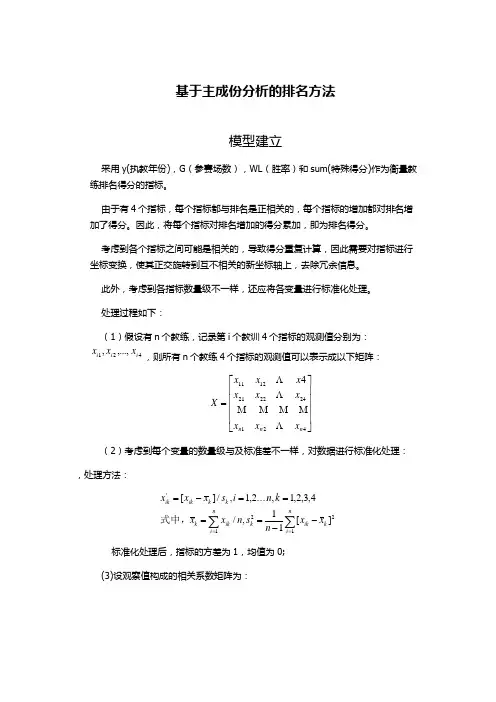
基于主成份分析的排名方法模型建立采用y(执教年份)，G （参赛场数），WL （胜率）和sum(特殊得分)作为衡量教练排名得分的指标。

由于有4个指标，每个指标都与排名是正相关的，每个指标的增加都对排名增加了得分。

因此，将每个指标对排名增加的得分累加，即为排名得分。

考虑到各个指标之间可能是相关的，导致得分重复计算，因此需要对指标进行坐标变换，使其正交旋转到互不相关的新坐标轴上，去除冗余信息。

此外，考虑到各指标数量级不一样，还应将各变量进行标准化处理。

处理过程如下：（1）假设有n 个教练，记录第i 个教训4个指标的观测值分别为：421,...,,i i i x x x ，则所有n 个教练4个指标的观测值可以表示成以下矩阵：⎥⎥⎥⎥⎦⎤⎢⎢⎢⎢⎣⎡=42124222112114n n n x x x x x x x x x X（2）考虑到每个变量的数量级与及标准差不一样，对数据进行标准化处理： ，处理方法：∑∑==--====-=n i k ik kni ik k k k ik ik x x n s n x x k n i s x x x 1221'][11,/4,3,2,1,....2,1,/][式中，标准化处理后，指标的方差为1，均值为0; (3)设观察值构成的相关系数矩阵为：⎥⎥⎥⎥⎦⎤⎢⎢⎢⎢⎣⎡=444241242221141211r r r r r r r r r R经标准化处理后的数据的相关系数为：)4,3,2,1,(,111''=-=∑=j i x x n r n k kj ki ij（4）对应于相关系数矩阵R ，求特征方程=-I R λ的p 个非负的特征值4321,,,λλλλ。

对应于特征值i λ的特征向量为：4,3,2,1,),,,('4321==i c c c c C i i i i i（5）求主成分。

由特征向量组成的4个主成分为：42211....X c X c X c F pi i i i +++=主成分4321,,,F F F F 之间相互无关，且它们的方差是递减的。

承诺书我们仔细阅读了《全国大学生数学建模竞赛章程》和《全国大学生数学建模竞赛参赛规则》（以下简称为“竞赛章程和参赛规则”，可从全国大学生数学建模竞赛网站下载）。

我们完全明白，在竞赛开始后参赛队员不能以任何方式（包括电话、电子邮件、网上咨询等）与队外的任何人（包括指导教师）研究、讨论与赛题有关的问题。

我们知道，抄袭别人的成果是违反竞赛章程和参赛规则的，如果引用别人的成果或其他公开的编号专用页赛区评阅编号（由赛区组委会评阅前进行编号）：对创意平板折叠桌的最优化设计摘要本文主要研究了创意平板折叠桌的相关问题。

对于问题一，首先，我们根据所提供的已知尺寸的长方形平板和桌面形状，桌高的要求，以圆桌面中心作为原点建立了相应的空间直角坐标系，分别求出了各个桌腿的长度，根据在折叠过程中，钢筋穿过的每个点距离桌面的高度相同这一性质，利用MATLAB程序计算出了每根木棒卡槽的长度和桌脚底端每个点的坐标，其中卡槽长度依次为（从最外侧开始，单位：cm）：0、4.3564、7.663、10.3684、目标任务建立数学模型讨论下列问题：1.给定长方形平板尺寸为120 cm×50 cm×3 cm，每根木条宽2.5 cm，连接桌腿木条的钢筋固定在桌腿最外侧木条的中心位置，折叠后桌子的高度为53 cm。

建立模型描述此折叠桌的动态变化过程，在此基础上给出此折叠桌的设计加工参数（例如，桌腿木条开槽的长度等）和桌脚边缘线（图4中红色曲线）的数学描述。

2.折叠桌的设计应做到产品稳固性好、加工方便、用材最少。

对于任意给定的折叠桌高度和圆形桌面直径的设计要求，讨论长方形平板材料和折叠桌的最优设计加工参数，例如，平板尺寸、钢筋位置、开槽长度等。

对于桌高70 cm，桌面直径80 cm的情形，确定最优设计加工参数。

3.公司计划开发一种折叠桌设计软件，根据客户任意设定的折叠桌高度、桌面边缘线的形状大小和桌脚边缘线的大致形状，给出所需平板材料的形状尺寸和切实可行的最优设计加工参数，使得生产的折叠桌尽可能接近客户所期望的形状。

高教社杯全国大学生数学建模竞赛承诺书我们仔细阅读了中国大学生数学建模竞赛的竞赛规则.我们完全明白，在竞赛开始后参赛队员不能以任何方式(包括、电子、网上咨询等)与队外的任何人(包括指导教师)研究、讨论与赛题有关的问题。

我们知道，抄袭别人的成果是违反竞赛规则的, 如果引用别人的成果或其他公开的资料(包括网上查到的资料)，必须按照规定的参考文献的表述方式在正文引用处和参考文献中明确列出。

我们重承诺，严格遵守竞赛规则，以保证竞赛的公正、公平性。

如有违反竞赛规则的行为，我们将受到严肃处理。

我们授权全国大学生数学建模竞赛组委会，可将我们的论文以任何形式进行公开展示(包括进行网上公示，在书籍、期刊和其他媒体进行正式或非正式发表等)。

我们参赛选择的题号是(从A/B/C/D中选择一项填写)： B我们的参赛报名号为(如果赛区设置报名号的话)：所属学校(请填写完整的全名)：农业大学参赛队员(打印并签名) ：1. 富顺2. 安明梅3. 熊万丹指导教师或指导教师组负责人(打印并签名)：指导组日期： 2014年 9 月 10 日赛区评阅编号(由赛区组委会评阅前进行编号)：2014高教社杯全国大学生数学建模竞赛编号专用页赛区评阅编号(由赛区组委会评阅前进行编号)：全国统一编号(由赛区组委会送交全国前编号)：全国评阅编号(由全国组委会评阅前进行编号)：太阳能小屋的设计摘要太阳能利用的重点是建筑，其应用方式包括利用太阳能为建筑物供热和供电，因此在设计电池时考虑太阳辐射强度、光线入射角、环境、建筑物所处的地理纬度、地区的气候与气象条件、安装部位及方式(贴附或架空)等对电池产电量的影响非常重要。

问题一，从题目给出的数据和收集到的资料出发，我们对所有数据进行处理，分析得到小屋每个面的总辐射强度，然后对其排序得到各个面的辐射强度的比例，利用模糊综合评判以及matlab模拟仿真得出问题的顶面最优值，小屋在35年的寿命期的发电量为343139.88KW,经济效益32万元，投资的回收年限14.33年。

2014高教社杯全国大学生数学建模竞赛承诺书我们仔细阅读了《全国大学生数学建模竞赛章程》和《全国大学生数学建模竞赛参赛规则》(以下简称为“竞赛章程和参赛规则”，可从全国大学生数学建模竞赛网站下载)。

我们完全明白，在竞赛开始后参赛队员不能以任何方式(包括电话、电子邮件、网上咨询等)与队外的任何人(包括指导教师)研究、讨论与赛题有关的问题。

我们知道，抄袭别人的成果是违反竞赛章程和参赛规则的，如果引用别人的成果或其他公开的资料(包括网上查到的资料)，必须按照规定的参考文献的表述方式在正文引用处和参考文献中明确列出。

我们郑重承诺，严格遵守竞赛章程和参赛规则，以保证竞赛的公正、公平性。

如有违反竞赛章程和参赛规则的行为，我们将受到严肃处理。

我们授权全国大学生数学建模竞赛组委会，可将我们的论文以任何形式进行公开展示(包括进行网上公示，在书籍、期刊和其他媒体进行正式或非正式发表等)。

我们参赛选择的题号是(从A/B/C/D中选择一项填写)：B我们的报名参赛队号为(8位数字组成的编号)：所属学校(请填写完整的全名)：参赛队员(打印并签名)：1.2.3.指导教师或指导教师组负责人(打印并签名)：(论文纸质版与电子版中的以上信息必须一致，只是电子版中无需签名。

以上内容请仔细核对，提交后将不再允许做任何修改。

如填写错误，论文可能被取消评奖资格。

)日期：年月日赛区评阅编号(由赛区组委会评阅前进行编号)：2014高教社杯全国大学生数学建模竞赛编号专用页赛区评阅编号(由赛区组委会评阅前进行编号)：全国评阅编号(由全国组委会评阅前进行编号)：创意平板折叠桌的设计摘要随着人类思维的不断进步，极具创意的作品也层出不穷。

本文对创意平板折叠桌进行分析，运用三维坐标对不同平板折叠桌的结构进行描述。

桌子外形由直纹曲面构成，桌面近似圆形，桌腿分成两组，每组各用一根钢筋将木条连接，钢筋两端分别固定在桌腿各组最外侧的两根木条上。

随着铰链的活动，折叠桌可以平摊成一张平板，折叠时，沿木条有空槽以保证滑动的自由度。