Density-based multifeature background subtraction with support vector machine
- 格式:pdf
- 大小:1.42 MB
- 文档页数:7

NuMicro®FamilyArm® ARM926EJ-S BasedNuMaker-HMI-N9H30User ManualEvaluation Board for NuMicro® N9H30 SeriesNUMAKER-HMI-N9H30 USER MANUALThe information described in this document is the exclusive intellectual property ofNuvoton Technology Corporation and shall not be reproduced without permission from Nuvoton.Nuvoton is providing this document only for reference purposes of NuMicro microcontroller andmicroprocessor based system design. Nuvoton assumes no responsibility for errors or omissions.All data and specifications are subject to change without notice.For additional information or questions, please contact: Nuvoton Technology Corporation.Table of Contents1OVERVIEW (5)1.1Features (7)1.1.1NuMaker-N9H30 Main Board Features (7)1.1.2NuDesign-TFT-LCD7 Extension Board Features (7)1.2Supporting Resources (8)2NUMAKER-HMI-N9H30 HARDWARE CONFIGURATION (9)2.1NuMaker-N9H30 Board - Front View (9)2.2NuMaker-N9H30 Board - Rear View (14)2.3NuDesign-TFT-LCD7 - Front View (20)2.4NuDesign-TFT-LCD7 - Rear View (21)2.5NuMaker-N9H30 and NuDesign-TFT-LCD7 PCB Placement (22)3NUMAKER-N9H30 AND NUDESIGN-TFT-LCD7 SCHEMATICS (24)3.1NuMaker-N9H30 - GPIO List Circuit (24)3.2NuMaker-N9H30 - System Block Circuit (25)3.3NuMaker-N9H30 - Power Circuit (26)3.4NuMaker-N9H30 - N9H30F61IEC Circuit (27)3.5NuMaker-N9H30 - Setting, ICE, RS-232_0, Key Circuit (28)NUMAKER-HMI-N9H30 USER MANUAL3.6NuMaker-N9H30 - Memory Circuit (29)3.7NuMaker-N9H30 - I2S, I2C_0, RS-485_6 Circuit (30)3.8NuMaker-N9H30 - RS-232_2 Circuit (31)3.9NuMaker-N9H30 - LCD Circuit (32)3.10NuMaker-N9H30 - CMOS Sensor, I2C_1, CAN_0 Circuit (33)3.11NuMaker-N9H30 - RMII_0_PF Circuit (34)3.12NuMaker-N9H30 - RMII_1_PE Circuit (35)3.13NuMaker-N9H30 - USB Circuit (36)3.14NuDesign-TFT-LCD7 - TFT-LCD7 Circuit (37)4REVISION HISTORY (38)List of FiguresFigure 1-1 Front View of NuMaker-HMI-N9H30 Evaluation Board (5)Figure 1-2 Rear View of NuMaker-HMI-N9H30 Evaluation Board (6)Figure 2-1 Front View of NuMaker-N9H30 Board (9)Figure 2-2 Rear View of NuMaker-N9H30 Board (14)Figure 2-3 Front View of NuDesign-TFT-LCD7 Board (20)Figure 2-4 Rear View of NuDesign-TFT-LCD7 Board (21)Figure 2-5 Front View of NuMaker-N9H30 PCB Placement (22)Figure 2-6 Rear View of NuMaker-N9H30 PCB Placement (22)Figure 2-7 Front View of NuDesign-TFT-LCD7 PCB Placement (23)Figure 2-8 Rear View of NuDesign-TFT-LCD7 PCB Placement (23)Figure 3-1 GPIO List Circuit (24)Figure 3-2 System Block Circuit (25)Figure 3-3 Power Circuit (26)Figure 3-4 N9H30F61IEC Circuit (27)Figure 3-5 Setting, ICE, RS-232_0, Key Circuit (28)Figure 3-6 Memory Circuit (29)Figure 3-7 I2S, I2C_0, RS-486_6 Circuit (30)Figure 3-8 RS-232_2 Circuit (31)Figure 3-9 LCD Circuit (32)NUMAKER-HMI-N9H30 USER MANUAL Figure 3-10 CMOS Sensor, I2C_1, CAN_0 Circuit (33)Figure 3-11 RMII_0_PF Circuit (34)Figure 3-12 RMII_1_PE Circuit (35)Figure 3-13 USB Circuit (36)Figure 3-14 TFT-LCD7 Circuit (37)List of TablesTable 2-1 LCD Panel Combination Connector (CON8) Pin Function (11)Table 2-2 Three Sets of Indication LED Functions (12)Table 2-3 Six Sets of User SW, Key Matrix Functions (12)Table 2-4 CMOS Sensor Connector (CON10) Function (13)Table 2-5 JTAG ICE Interface (J2) Function (14)Table 2-6 Expand Port (CON7) Function (16)Table 2-7 UART0 (J3) Function (16)Table 2-8 UART2 (J6) Function (16)Table 2-9 RS-485_6 (SW6~8) Function (17)Table 2-10 Power on Setting (SW4) Function (17)Table 2-11 Power on Setting (S2) Function (17)Table 2-12 Power on Setting (S3) Function (17)Table 2-13 Power on Setting (S4) Function (17)Table 2-14 Power on Setting (S5) Function (17)Table 2-15 Power on Setting (S7/S6) Function (18)Table 2-16 Power on Setting (S9/S8) Function (18)Table 2-17 CMOS Sensor Connector (CON9) Function (19)Table 2-18 CAN_0 (SW9~10) Function (19)NUMAKER-HMI-N9H30 USER MANUAL1 OVERVIEWThe NuMaker-HMI-N9H30 is an evaluation board for GUI application development. The NuMaker-HMI-N9H30 consists of two parts: a NuMaker-N9H30 main board and a NuDesign-TFT-LCD7 extensionboard. The NuMaker-HMI-N9H30 is designed for project evaluation, prototype development andvalidation with HMI (Human Machine Interface) function.The NuMaker-HMI-N9H30 integrates touchscreen display, voice input/output, rich serial port serviceand I/O interface, providing multiple external storage methods.The NuDesign-TFT-LCD7 can be plugged into the main board via the DIN_32x2 extension connector.The NuDesign-TFT-LCD7 includes one 7” LCD which the resolution is 800x480 with RGB-24bits andembedded the 4-wires resistive type touch panel.Figure 1-1 Front View of NuMaker-HMI-N9H30 Evaluation BoardNUMAKER-HMI-N9H30 USER MANUAL Figure 1-2 Rear View of NuMaker-HMI-N9H30 Evaluation Board1.1 Features1.1.1 NuMaker-N9H30 Main Board Features●N9H30F61IEC chip: LQFP216 pin MCP package with DDR (64 MB)●SPI Flash using W25Q256JVEQ (32 MB) booting with quad mode or storage memory●NAND Flash using W29N01HVSINA (128 MB) booting or storage memory●One Micro-SD/TF card slot served either as a SD memory card for data storage or SDIO(Wi-Fi) device●Two sets of COM ports:–One DB9 RS-232 port with UART_0 used 75C3232E transceiver chip can be servedfor function debug and system development.–One DB9 RS-232 port with UART_2 used 75C3232E transceiver chip for userapplication●22 GPIO expansion ports, including seven sets of UART functions●JTAG interface provided for software development●Microphone input and Earphone/Speaker output with 24-bit stereo audio codec(NAU88C22) for I2S interfaces●Six sets of user-configurable push button keys●Three sets of LEDs for status indication●Provides SN65HVD230 transceiver chip for CAN bus communication●Provides MAX3485 transceiver chip for RS-485 device connection●One buzzer device for program applicationNUMAKER-HMI-N9H30 USER MANUAL●Two sets of RJ45 ports with Ethernet 10/100 Mbps MAC used IP101GR PHY chip●USB_0 that can be used as Device/HOST and USB_1 that can be used as HOSTsupports pen drives, keyboards, mouse and printers●Provides over-voltage and over current protection used APL3211A chip●Retain RTC battery socket for CR2032 type and ADC0 detect battery voltage●System power could be supplied by DC-5V adaptor or USB VBUS1.1.2 NuDesign-TFT-LCD7 Extension Board Features●7” resolution 800x480 4-wire resistive touch panel for 24-bits RGB888 interface●DIN_32x2 extension connector1.2 Supporting ResourcesFor sample codes and introduction about NuMaker-N9H30, please refer to N9H30 BSP:https:///products/gui-solution/gui-platform/numaker-hmi-n9h30/?group=Software&tab=2Visit NuForum for further discussion about the NuMaker-HMI-N9H30:/viewforum.php?f=31 NUMAKER-HMI-N9H30 USER MANUALNUMAKER-HMI-N9H30 USER MANUAL2 NUMAKER-HMI-N9H30 HARDWARE CONFIGURATION2.1 NuMaker-N9H30 Board - Front View Combination Connector (CON8)6 set User SWs (K1~6)3set Indication LEDs (LED1~3)Power Supply Switch (SW_POWER1)Audio Codec(U10)Microphone(M1)NAND Flash(U9)RS-232 Transceiver(U6, U12)RS-485 Transceiver(U11)CAN Transceiver (U13)Figure 2-1 Front View of NuMaker-N9H30 BoardFigure 2-1 shows the main components and connectors from the front side of NuMaker-N9H30 board. The following lists components and connectors from the front view:NuMaker-N9H30 board and NuDesign-TFT-LCD7 board combination connector (CON8). This panel connector supports 4-/5-wire resistive touch or capacitance touch panel for 24-bits RGB888 interface.Connector GPIO pin of N9H30 FunctionCON8.1 - Power 3.3VCON8.2 - Power 3.3VCON8.3 GPD7 LCD_CSCON8.4 GPH3 LCD_BLENCON8.5 GPG9 LCD_DENCON8.7 GPG7 LCD_HSYNCCON8.8 GPG6 LCD_CLKCON8.9 GPD15 LCD_D23(R7)CON8.10 GPD14 LCD_D22(R6)CON8.11 GPD13 LCD_D21(R5)CON8.12 GPD12 LCD_D20(R4)CON8.13 GPD11 LCD_D19(R3)CON8.14 GPD10 LCD_D18(R2)CON8.15 GPD9 LCD_D17(R1)CON8.16 GPD8 LCD_D16(R0)CON8.17 GPA15 LCD_D15(G7)CON8.18 GPA14 LCD_D14(G6)CON8.19 GPA13 LCD_D13(G5)CON8.20 GPA12 LCD_D12(G4)CON8.21 GPA11 LCD_D11(G3)CON8.22 GPA10 LCD_D10(G2)CON8.23 GPA9 LCD_D9(G1) NUMAKER-HMI-N9H30 USER MANUALCON8.24 GPA8 LCD_D8(G0)CON8.25 GPA7 LCD_D7(B7)CON8.26 GPA6 LCD_D6(B6)CON8.27 GPA5 LCD_D5(B5)CON8.28 GPA4 LCD_D4(B4)CON8.29 GPA3 LCD_D3(B3)CON8.30 GPA2 LCD_D2(B2)CON8.31 GPA1 LCD_D1(B1)CON8.32 GPA0 LCD_D0(B0)CON8.33 - -CON8.34 - -CON8.35 - -CON8.36 - -CON8.37 GPB2 LCD_PWMCON8.39 - VSSCON8.40 - VSSCON8.41 ADC7 XPCON8.42 ADC3 VsenCON8.43 ADC6 XMCON8.44 ADC4 YMCON8.45 - -CON8.46 ADC5 YPCON8.47 - VSSCON8.48 - VSSCON8.49 GPG0 I2C0_CCON8.50 GPG1 I2C0_DCON8.51 GPG5 TOUCH_INTCON8.52 - -CON8.53 - -CON8.54 - -CON8.55 - -NUMAKER-HMI-N9H30 USER MANUAL CON8.56 - -CON8.57 - -CON8.58 - -CON8.59 - VSSCON8.60 - VSSCON8.61 - -CON8.62 - -CON8.63 - Power 5VCON8.64 - Power 5VTable 2-1 LCD Panel Combination Connector (CON8) Pin Function●Power supply switch (SW_POWER1): System will be powered on if the SW_POWER1button is pressed●Three sets of indication LEDs:LED Color DescriptionsLED1 Red The system power will beterminated and LED1 lightingwhen the input voltage exceeds5.7V or the current exceeds 2A.LED2 Green Power normal state.LED3 Green Controlled by GPH2 pin Table 2-2 Three Sets of Indication LED Functions●Six sets of user SW, Key Matrix for user definitionKey GPIO pin of N9H30 FunctionK1 GPF10 Row0 GPB4 Col0K2 GPF10 Row0 GPB5 Col1K3 GPE15 Row1 GPB4 Col0K4 GPE15 Row1 GPB5 Col1K5 GPE14 Row2 GPB4 Col0K6GPE14 Row2GPB5 Col1 Table 2-3 Six Sets of User SW, Key Matrix Functions●NAND Flash (128 MB) with Winbond W29N01HVS1NA (U9)●Microphone (M1): Through Nuvoton NAU88C22 chip sound input●Audio CODEC chip (U10): Nuvoton NAU88C22 chip connected to N9H30 using I2Sinterface–SW6/SW7/SW8: 1-2 short for RS-485_6 function and connected to 2P terminal (CON5and J5)–SW6/SW7/SW8: 2-3 short for I2S function and connected to NAU88C22 (U10).●CMOS Sensor connector (CON10, SW9~10)–SW9~10: 1-2 short for CAN_0 function and connected to 2P terminal (CON11)–SW9~10: 2-3 short for CMOS sensor function and connected to CMOS sensorconnector (CON10)Connector GPIO pin of N9H30 FunctionCON10.1 - VSSCON10.2 - VSSNUMAKER-HMI-N9H30 USER MANUALCON10.3 - Power 3.3VCON10.4 - Power 3.3VCON10.5 - -CON10.6 - -CON10.7 GPI4 S_PCLKCON10.8 GPI3 S_CLKCON10.9 GPI8 S_D0CON10.10 GPI9 S_D1CON10.11 GPI10 S_D2CON10.12 GPI11 S_D3CON10.13 GPI12 S_D4CON10.14 GPI13 S_D5CON10.15 GPI14 S_D6CON10.16 GPI15 S_D7CON10.17 GPI6 S_VSYNCCON10.18 GPI5 S_HSYNCCON10.19 GPI0 S_PWDNNUMAKER-HMI-N9H30 USER MANUAL CON10.20 GPI7 S_nRSTCON10.21 GPG2 I2C1_CCON10.22 GPG3 I2C1_DCON10.23 - VSSCON10.24 - VSSTable 2-4 CMOS Sensor Connector (CON10) FunctionNUMAKER-HMI-N9H30 USER MANUAL2.2NuMaker-N9H30 Board - Rear View5V In (CON1)RS-232 DB9 (CON2,CON6)Expand Port (CON7)Speaker Output (J4)Earphone Output (CON4)Buzzer (BZ1)System ResetSW (SW5)SPI Flash (U7,U8)JTAG ICE (J2)Power ProtectionIC (U1)N9H30F61IEC (U5)Micro SD Slot (CON3)RJ45 (CON12, CON13)USB1 HOST (CON15)USB0 Device/Host (CON14)CAN_0 Terminal (CON11)CMOS Sensor Connector (CON9)Power On Setting(SW4, S2~S9)RS-485_6 Terminal (CON5)RTC Battery(BT1)RMII PHY (U14,U16)Figure 2-2 Rear View of NuMaker-N9H30 BoardFigure 2-2 shows the main components and connectors from the rear side of NuMaker-N9H30 board. The following lists components and connectors from the rear view:● +5V In (CON1): Power adaptor 5V input ●JTAG ICE interface (J2) ConnectorGPIO pin of N9H30Function J2.1 - Power 3.3V J2.2 GPJ4 nTRST J2.3 GPJ2 TDI J2.4 GPJ1 TMS J2.5 GPJ0 TCK J2.6 - VSS J2.7 GPJ3 TD0 J2.8-RESETTable 2-5 JTAG ICE Interface (J2) Function●SPI Flash (32 MB) with Winbond W25Q256JVEQ (U7); only one (U7 or U8) SPI Flashcan be used●System Reset (SW5): System will be reset if the SW5 button is pressed●Buzzer (BZ1): Control by GPB3 pin of N9H30●Speaker output (J4): Through the NAU88C22 chip sound output●Earphone output (CON4): Through the NAU88C22 chip sound output●Expand port for user use (CON7):Connector GPIO pin of N9H30 FunctionCON7.1 - Power 3.3VCON7.2 - Power 3.3VCON7.3 GPE12 UART3_TXDCON7.4 GPH4 UART1_TXDCON7.5 GPE13 UART3_RXDCON7.6 GPH5 UART1_RXDCON7.7 GPB0 UART5_TXDCON7.8 GPH6 UART1_RTSCON7.9 GPB1 UART5_RXDCON7.10 GPH7 UART1_CTSCON7.11 GPI1 UART7_TXDNUMAKER-HMI-N9H30 USER MANUAL CON7.12 GPH8 UART4_TXDCON7.13 GPI2 UART7_RXDCON7.14 GPH9 UART4_RXDCON7.15 - -CON7.16 GPH10 UART4_RTSCON7.17 - -CON7.18 GPH11 UART4_CTSCON7.19 - VSSCON7.20 - VSSCON7.21 GPB12 UART10_TXDCON7.22 GPH12 UART8_TXDCON7.23 GPB13 UART10_RXDCON7.24 GPH13 UART8_RXDCON7.25 GPB14 UART10_RTSCON7.26 GPH14 UART8_RTSCON7.27 GPB15 UART10_CTSCON7.28 GPH15 UART8_CTSCON7.29 - Power 5VCON7.30 - Power 5VTable 2-6 Expand Port (CON7) Function●UART0 selection (CON2, J3):–RS-232_0 function and connected to DB9 female (CON2) for debug message output.–GPE0/GPE1 connected to 2P terminal (J3).Connector GPIO pin of N9H30 Function J3.1 GPE1 UART0_RXDJ3.2 GPE0 UART0_TXDTable 2-7 UART0 (J3) Function●UART2 selection (CON6, J6):–RS-232_2 function and connected to DB9 female (CON6) for debug message output –GPF11~14 connected to 4P terminal (J6)Connector GPIO pin of N9H30 Function J6.1 GPF11 UART2_TXDJ6.2 GPF12 UART2_RXDJ6.3 GPF13 UART2_RTSJ6.4 GPF14 UART2_CTSTable 2-8 UART2 (J6) Function●RS-485_6 selection (CON5, J5, SW6~8):–SW6~8: 1-2 short for RS-485_6 function and connected to 2P terminal (CON5 and J5) –SW6~8: 2-3 short for I2S function and connected to NAU88C22 (U10)Connector GPIO pin of N9H30 FunctionSW6:1-2 shortGPG11 RS-485_6_DISW6:2-3 short I2S_DOSW7:1-2 shortGPG12 RS-485_6_ROSW7:2-3 short I2S_DISW8:1-2 shortGPG13 RS-485_6_ENBSW8:2-3 short I2S_BCLKNUMAKER-HMI-N9H30 USER MANUALTable 2-9 RS-485_6 (SW6~8) FunctionPower on setting (SW4, S2~9).SW State FunctionSW4.2/SW4.1 ON/ON Boot from USB SW4.2/SW4.1 ON/OFF Boot from eMMC SW4.2/SW4.1 OFF/ON Boot from NAND Flash SW4.2/SW4.1 OFF/OFF Boot from SPI Flash Table 2-10 Power on Setting (SW4) FunctionSW State FunctionS2 Short System clock from 12MHzcrystalS2 Open System clock from UPLL output Table 2-11 Power on Setting (S2) FunctionSW State FunctionS3 Short Watchdog Timer OFFS3 Open Watchdog Timer ON Table 2-12 Power on Setting (S3) FunctionSW State FunctionS4 Short GPJ[4:0] used as GPIO pinS4Open GPJ[4:0] used as JTAG ICEinterfaceTable 2-13 Power on Setting (S4) FunctionSW State FunctionS5 Short UART0 debug message ONS5 Open UART0 debug message OFFTable 2-14 Power on Setting (S5) FunctionSW State FunctionS7/S6 Short/Short NAND Flash page size 2KBS7/S6 Short/Open NAND Flash page size 4KBS7/S6 Open/Short NAND Flash page size 8KBNUMAKER-HMI-N9H30 USER MANUALS7/S6 Open/Open IgnoreTable 2-15 Power on Setting (S7/S6) FunctionSW State FunctionS9/S8 Short/Short NAND Flash ECC type BCH T12S9/S8 Short/Open NAND Flash ECC type BCH T15S9/S8 Open/Short NAND Flash ECC type BCH T24S9/S8 Open/Open IgnoreTable 2-16 Power on Setting (S9/S8) FunctionCMOS Sensor connector (CON9, SW9~10)–SW9~10: 1-2 short for CAN_0 function and connected to 2P terminal (CON11).–SW9~10: 2-3 short for CMOS sensor function and connected to CMOS sensorconnector (CON9).Connector GPIO pin of N9H30 FunctionCON9.1 - VSSCON9.2 - VSSCON9.3 - Power 3.3VCON9.4 - Power 3.3V NUMAKER-HMI-N9H30 USER MANUALCON9.5 - -CON9.6 - -CON9.7 GPI4 S_PCLKCON9.8 GPI3 S_CLKCON9.9 GPI8 S_D0CON9.10 GPI9 S_D1CON9.11 GPI10 S_D2CON9.12 GPI11 S_D3CON9.13 GPI12 S_D4CON9.14 GPI13 S_D5CON9.15 GPI14 S_D6CON9.16 GPI15 S_D7CON9.17 GPI6 S_VSYNCCON9.18 GPI5 S_HSYNCCON9.19 GPI0 S_PWDNCON9.20 GPI7 S_nRSTCON9.21 GPG2 I2C1_CCON9.22 GPG3 I2C1_DCON9.23 - VSSCON9.24 - VSSTable 2-17 CMOS Sensor Connector (CON9) Function●CAN_0 Selection (CON11, SW9~10):–SW9~10: 1-2 short for CAN_0 function and connected to 2P terminal (CON11) –SW9~10: 2-3 short for CMOS sensor function and connected to CMOS sensor connector (CON9, CON10)SW GPIO pin of N9H30 FunctionSW9:1-2 shortGPI3 CAN_0_RXDSW9:2-3 short S_CLKSW10:1-2 shortGPI4 CAN_0_TXDSW10:2-3 short S_PCLKTable 2-18 CAN_0 (SW9~10) Function●USB0 Device/HOST Micro-AB connector (CON14), where CON14 pin4 ID=1 is Device,ID=0 is HOST●USB1 for USB HOST with Type-A connector (CON15)●RJ45_0 connector with LED indicator (CON12), RMII PHY with IP101GR (U14)●RJ45_1 connector with LED indicator (CON13), RMII PHY with IP101GR (U16)●Micro-SD/TF card slot (CON3)●SOC CPU: Nuvoton N9H30F61IEC (U5)●Battery power for RTC 3.3V powered (BT1, J1), can detect voltage by ADC0●RTC power has 3 sources:–Share with 3.3V I/O power–Battery socket for CR2032 (BT1)–External connector (J1)●Board version 2.1NUMAKER-HMI-N9H30 USER MANUAL2.3 NuDesign-TFT-LCD7 -Front ViewFigure 2-3 Front View of NuDesign-TFT-LCD7 BoardFigure 2-3 shows the main components and connectors from the Front side of NuDesign-TFT-LCD7board.7” resolution 800x480 4-W resistive touch panel for 24-bits RGB888 interface2.4 NuDesign-TFT-LCD7 -Rear ViewFigure 2-4 Rear View of NuDesign-TFT-LCD7 BoardFigure 2-4 shows the main components and connectors from the rear side of NuDesign-TFT-LCD7board.NuMaker-N9H30 and NuDesign-TFT-LCD7 combination connector (CON1).NUMAKER-HMI-N9H30 USER MANUAL 2.5 NuMaker-N9H30 and NuDesign-TFT-LCD7 PCB PlacementFigure 2-5 Front View of NuMaker-N9H30 PCB PlacementFigure 2-6 Rear View of NuMaker-N9H30 PCB PlacementNUMAKER-HMI-N9H30 USER MANUALFigure 2-7 Front View of NuDesign-TFT-LCD7 PCB PlacementFigure 2-8 Rear View of NuDesign-TFT-LCD7 PCB Placement3 NUMAKER-N9H30 AND NUDESIGN-TFT-LCD7 SCHEMATICS3.1 NuMaker-N9H30 - GPIO List CircuitFigure 3-1 shows the N9H30F61IEC GPIO list circuit.Figure 3-1 GPIO List Circuit NUMAKER-HMI-N9H30 USER MANUAL3.2 NuMaker-N9H30 - System Block CircuitFigure 3-2 shows the System Block Circuit.NUMAKER-HMI-N9H30 USER MANUALFigure 3-2 System Block Circuit3.3 NuMaker-N9H30 - Power CircuitFigure 3-3 shows the Power Circuit.NUMAKER-HMI-N9H30 USER MANUALFigure 3-3 Power Circuit3.4 NuMaker-N9H30 - N9H30F61IEC CircuitFigure 3-4 shows the N9H30F61IEC Circuit.Figure 3-4 N9H30F61IEC CircuitNUMAKER-HMI-N9H30 USER MANUAL3.5 NuMaker-N9H30 - Setting, ICE, RS-232_0, Key CircuitFigure 3-5 shows the Setting, ICE, RS-232_0, Key Circuit.NUMAKER-HMI-N9H30 USER MANUALFigure 3-5 Setting, ICE, RS-232_0, Key Circuit3.6 NuMaker-N9H30 - Memory CircuitFigure 3-6 shows the Memory Circuit.NUMAKER-HMI-N9H30 USER MANUALFigure 3-6 Memory Circuit3.7 NuMaker-N9H30 - I2S, I2C_0, RS-485_6 CircuitFigure 3-7 shows the I2S, I2C_0, RS-486_6 Circuit.NUMAKER-HMI-N9H30 USER MANUALFigure 3-7 I2S, I2C_0, RS-486_6 Circuit3.8 NuMaker-N9H30 - RS-232_2 CircuitFigure 3-8 shows the RS-232_2 Circuit.NUMAKER-HMI-N9H30 USER MANUALFigure 3-8 RS-232_2 Circuit3.9 NuMaker-N9H30 - LCD CircuitFigure 3-9 shows the LCD Circuit.NUMAKER-HMI-N9H30 USER MANUALFigure 3-9 LCD Circuit3.10 NuMaker-N9H30 - CMOS Sensor, I2C_1, CAN_0 CircuitFigure 3-10 shows the CMOS Sensor,I2C_1, CAN_0 Circuit.NUMAKER-HMI-N9H30 USER MANUALFigure 3-10 CMOS Sensor, I2C_1, CAN_0 Circuit3.11 NuMaker-N9H30 - RMII_0_PF CircuitFigure 3-11 shows the RMII_0_RF Circuit.NUMAKER-HMI-N9H30 USER MANUALFigure 3-11 RMII_0_PF Circuit3.12 NuMaker-N9H30 - RMII_1_PE CircuitFigure 3-12 shows the RMII_1_PE Circuit.NUMAKER-HMI-N9H30 USER MANUALFigure 3-12 RMII_1_PE Circuit3.13 NuMaker-N9H30 - USB CircuitFigure 3-13 shows the USB Circuit.NUMAKER-HMI-N9H30 USER MANUALFigure 3-13 USB Circuit3.14 NuDesign-TFT-LCD7 - TFT-LCD7 CircuitFigure 3-14 shows the TFT-LCD7 Circuit.Figure 3-14 TFT-LCD7 CircuitNUMAKER-HMI-N9H30 USER MANUAL4 REVISION HISTORYDate Revision Description2022.03.24 1.00 Initial version NUMAKER-HMI-N9H30 USER MANUALNUMAKER-HMI-N9H30 USER MANUALImportant NoticeNuvoton Products are neither intended nor warranted for usage in systems or equipment, anymalfunction or failure of which may cause loss of human life, bodily injury or severe propertydamage. Such applications are deemed, “Insecure Usage”.Insecure usage includes, but is not limited to: equipment for surgical implementation, atomicenergy control instruments, airplane or spaceship instruments, the control or operation ofdynamic, brake or safety systems designed for vehicular use, traffic signal instruments, all typesof safety devices, and other applications intended to support or sustain life.All Insecure Usage shall be made at customer’s risk, and in the event that third parties lay claimsto Nuvoton as a result of customer’s Insecure Usage, custome r shall indemnify the damagesand liabilities thus incurred by Nuvoton.。

density方案引言在计算机图形学和图像处理领域,density是一个关键概念,经常用于描述像素密度、线段密度、采样密度等。
针对不同应用场景,设计合适的density方案可以有效提高图像的清晰度和质量。
本文将介绍density的定义和分类,并结合实际应用场景,提出一种适用于不同设备的density方案。
1. density的定义1.1 像素密度像素密度通常用单位长度上的像素数量来衡量,常见表示为DPI(每英寸像素数)或PPI(每英寸像素数)。
它用于描述图像的清晰度,像素密度越高,图像越清晰。
1.2 线段密度线段密度指每单位长度上表示线段的像素数。
在绘制曲线或边缘时,较高的线段密度可以提高图像的光滑度和精细度。
1.3 采样密度采样密度表示在离散数据中取样的频率。
在信号处理和图像重建中,采样密度决定了信号的保真度和细节还原能力。
2. density的分类根据应用场景和使用对象的不同,density可以分为像素密度、线段密度和采样密度三个类别。
2.1 像素密度像素密度适用于显示设备,例如计算机显示器、移动设备屏幕等。
不同设备具有不同的像素密度,合理设置像素密度可以使图像在不同设备上保持一致的尺寸和清晰度。
在移动设备上,由于屏幕尺寸和分辨率的多样性,像素密度适用于确保应用在不同设备上的显示效果一致。
在设计移动应用时,可以使用独立像素单位(dp或dip)来忽略不同设备上的像素密度差异,从而实现自适应布局。
2.2 线段密度线段密度适用于绘图、图形渲染等领域。
在绘制平滑曲线时,较高的线段密度可以减少锯齿状边缘,提高图像质量。
对于打印、绘画等需要高精度输出的应用,也需要考虑线段密度以保证图像的视觉效果。
2.3 采样密度采样密度适用于信号处理、图像处理等领域。
在数字信号处理中,合适的采样密度可以保证信号在离散形式下的还原精度。
在图像处理中,采样密度决定了图像的细节保留程度和色彩还原度。
3. 适用于不同设备的density方案根据不同设备和应用场景的需求,我们提出以下方案来处理density问题。

拉曼晶圆lt衬底材料界面
拉曼晶圆LT衬底材料界面通常指的是衬底的表面和材料之间
的界面。
由于拉曼晶圆LT衬底材料通常是通过化学气相沉积
或分子束外延等方式生长在衬底上的,因此衬底材料界面对于拉曼晶圆的性能和质量起着至关重要的作用。
在拉曼晶圆LT衬底材料界面上,常常存在着应力、晶格失配、缺陷等问题。
这些问题会导致材料的晶格畸变和结构杂质的形成,影响拉曼晶圆的光电性能。
为了解决这些问题,可以通过界面控制和应力调控技术来优化拉曼晶圆的界面结构和性能。
界面控制技术包括衬底前处理、表面清洁和预测等方法,用于改善拉曼晶圆LT衬底材料的表面质量和界面结构。
应力调控
技术则是通过在衬底生长过程中控制材料的应力分布和缓解晶格失配,来减少界面应力和缺陷的形成。
通过界面控制和应力调控技术,可以改善拉曼晶圆LT衬底材
料的界面结构和质量,提高拉曼晶圆的光电性能和稳定性。
这对于应用于光电子器件和半导体器件等领域具有重要的意义。

基于深度学习的衬衫定制设计作者:贾群喜张伟民罗依平来源:《电脑知识与技术》2021年第31期摘要:为了深度学习更好地在衬衫定制设计中的应用,解决衬衫定制中人体参数识别不准、价格昂贵和标准不统一等问题,提出了一种基于深度学习的衬衫定制设计方法。
利用Deeplab V3图像分割神经网络,在自主建立数据集的基础上,进行人体模型和背景的分割,结合人体特征点的方法进行人体尺寸的拟合,同时考虑衬衫的个性化定制,并进行真人试穿检验。
实验结果综合得分在6.0以上,表明可以该方法进行衬衫个性化定制方面表现良好,并在具有一定的应用价值。
关键词:衬衫;定制;Deeplab V3;特征点提取;人体尺寸拟合中图分类号:TP18 文献标识码:A文章编号:1009-3044(2021)31-0109-03Shirt Customization Design Based on Deep LearningJIA Qun-xi,ZHANG Wei-min,LUO Yi-ping(Luoyang Institute of Science and Technology, Luoyang 471000, China)Abstract:In order to better apply deep learning in shirt customization design and solve the problems of inaccurate human parameter identification, high price and inconsistent standards in shirt customization, a design method of shirt customization based on deep learning is proposed. The Deeplab V3 image segmentation neural network is used to segment the human model and background on the basis of independently establishing the data set. The fitting of human size is carried out by combining the method of human feature points. At the same time, the personalized customization of shirts is considered, and the real-life test is carried out. The comprehensive score of the experimental results is above 6.0, indicating that the method can perform well in the personalized customization of shirts, and has certain application value.Key words:Shirt ; customization; Deeplab V3 ; feature point extraction ; Body size fitting目前,伴隨着生活水平的提升,消费者对于服装的个性化、差异化要求也在逐步提升。

第37卷第4期2022年4月Vol.37No.4Apr.2022液晶与显示Chinese Journal of Liquid Crystals and Displays氮化硅膜层对侧视角白画面色偏的影响及发红改善叶成枝*,操彬彬,吕艳明,马力,安晖,彭俊林,冯耀耀,杨增乾,栗芳芳,陆相晚,李恒滨(合肥鑫晟光电科技有限公司,安徽合肥230001)摘要:研究了TFT基板中氮化硅膜层对TFT-LCD终端产品侧视角白画面色偏的影响,填补了TFT膜层与TFT-LCD 侧视角白画面色偏的研究欠缺,为类似的光学色度不良改善提供了有益的参考。
通过大量的实验测试和仿真模拟,探索了氧化硅膜层厚度对侧视角白画面色偏的影响规律。
结果表明,氮化硅膜层是一个影响色偏量和色偏方向的关键因素,其中栅极绝缘层(GI)和第一钝化绝缘层(PVX1)对色偏的影响较大,而第二钝化绝缘层(PVX2)对色偏的影响较小,氮化硅厚度与白画面侧视角色偏程度呈非线性相关。
以某款HADS产品为例,其中氮化硅膜层包括栅极绝缘层(320 nm)、第一钝化绝缘层(100nm)和第二钝化绝缘层(200nm)。
基于单因子实验结果和模拟结果,综合考虑电学特性和产能影响,采用PVX1140nm作为改善条件,对侧视角白画面发红改善有效,即宏观观察无发红现象且实测数据都满足产品规格。
关键词:薄膜晶体管液晶显示器;氮化硅膜层;光学色度;侧视角色偏;全白画面中图分类号:TN141.9;O439doi:10.37188/CJLCD.2021-0284Influence of SiN x film on off-angle color shift of white screen andreddish improvementYE Cheng-zhi*,CAO Bin-bin,LYU Yan-ming,MA Li,AN Hui,PENG Jun-lin,FENG Yao-yao,YANG Zeng-qian,LI Fang-fang,LU Xiang-wan,LI Heng-bin(Hefei Xinsheng Optoelectronics Technology Co.,Ltd.,Hefei230001,China)Abstract:Research on the relationship of SiNx film to off-angle color shift on white screen is carried out. The research in this paper fills in the lack of research of correlation between TFT film and off-angle color shift of TFT-LCD,and provides a useful reference for the improvement of similar optical chromaticity de‐fects in other products.Through experimental measurement and software simulation,the influence of the thickness of the silicon nitride film on the color shift coordinates is explored.Experimental results show that the silicon nitride film layer is a key factor affecting the color shift,GI and PVX1have a greater impact on color shift,while PVX2has a little impact on color shift,and the thickness of the SiN x is nonlinearly re‐lated to off-angle color shift on white screen.Taking a HADS product for example,the SiN x film layer in‐cludes gate insulating layer(320nm),1st passivation insulator layer(100nm),2nd passivation insulator layer(200nm).Based on single-factor experimental and simulation results,comprehensively considering 文章编号:1007-2780(2022)04-0467-08收稿日期:2021-11-11;修订日期:2022-02-17.*通信联系人,E-mail:yechengzhi@第37卷液晶与显示the electrical characteristics and production capacity,the reddish on white screen from the viewing angle is improved effectively when PVX1140nm is used as the condition.That means there is no reddish by mac‐roscopic observation and the measured data meets product specifications.Key words:thin film transistor liquid crystal display;SiNx film;optical chromaticity;off-angle color shift;white display1引言薄膜晶体管液晶显示技术(Thin Film Tran‐sistor Liquid Crystal Display,TFT-LCD)是目前平板显示市场主流的显示技术之一[1]。
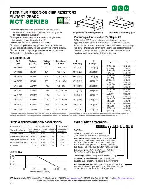
MCT SERIESSPECIFICATIONSTYPICAL PERFORMANCE CHARACTERISTICSTHICK FILM PRECISION CHIP RESISTORS MILITARY GRADEChoice of termination materials: 100% tin plated nickel barrier is standard (palladium silver, gold, or tin-lead solder is available)Wraparound termination is standard, single sided termination is available (Option ‘S’)Wide resistance range: 0.1Ω to 100M Ω100% Group A screening per MIL-R-55342 available Wide design flexibility for use with hybrid or smd circuitry Custom sizes, high surge, untrimmed chips available Backside metalization availablePrecision performance to 0.1% 50ppm/°C!RCD series MCT chip resistors are designed to meetapplicable performance requirements of MIL-PRF-553421.Variety of sizes and termination materials allows wide design flexibility. Palladium silver terminations are recommended for use with conductive epoxy, gold is recommended for wire bonding, and tin plated nickel for soldering.* Dimension given is for single face termination. Add .004” [.1mm] for wraparound termination. ** Wattage based on mounting to ceramic substrate, derate by 25% if mounted to a glass epoxy P .C.B.1 Military p/n’s are given for reference only and do not imply qualification or exact interchangeability. 2 Dimension “t” (underside termination width) applies only to termination type WSingle Face Termination (Opt. S)Wraparound Termination (standard)D C R e p y T e g a t t a W **C °07@e g a t l o V g n i t a R e c n a t s i s e R e g n a R *L ]2.0[800.±W ]2.0[800.±t 2*T 2040T C M W M 05V 0301ΩM 1-]0.1[930.]15.[020.500.±210.]31.±3.[600.±410.]51.±53.[5050T C M W M 001V 051ΩM 01-]72.1[050.]72.1[050.700.±410.]81.±53.[600.±810.]51.±54.[3060T C M W M 001V 041.0ΩM 001-]35.1[060.]67.[030.600.±210.]51.±3.[600.±810.]51.±54.[5080T C M W M 051V 071.0ΩM 001-]19.1[570.]72.1[050.800.±610.]2.±4.[600.±810.]51.±05.[5001T C M W M 002V 0011ΩM 02-]45.2[001.]72.1[050.800.±810.]2.±54.[600.±020.]51.±05.[6021T C M W M 052V 5211.0ΩM 001-]51.3[421.]55.1[160.800.±020.]2.±5.[600.±020.]51.±05.[5051T C M W M 052V 5211ΩM 01-]18.3[051.]72.1[050.010±020.]52.±5.[600.±020.]51.±05.[0121T C M W M 005V 0511.0ΩM 001-]51.3[421.]45.2[001.010.±020.]52.±5.[600.±020.]51.±05.[0102T C M W M 008V 0511.0ΩM 001-]0.5[691.]45.2[001.010.±020.]52.±5.[600.±020.]51.±05.[2152T C M WM 0001V0021.0ΩM001-]3.6[842.]81.3[521.010.±020.]52.±5.[600.±020.]51.±05.[c i t s i r e t c a r a h C 01ΩM 1o t Ωe g n a r 01<ΩM 1>,Ωt n e i c i f f e o C .p m e T m p p 003±)d r a d n a t s (m p p 001±).t p o (m p p 05±).t p o (m p p 004±)d r a d n a t s (k c o h S l a m r e h T %5.0%5.0%5.0%57.0d a o l r e v O e m i T t r o h S %5.0%52.0%52.0%1e r u s o p x E .p m e T h g i H %5.0%5.0%5.0%57.0e c n a t s i s e R e r u t s i o M %5.0%5.0%5.0%5.1ef i L d a o L %0.1%5.0%5.0%5.1RESISTORS CAPACITOR S C OILS DELAY LINES35 70 105 140 150 175% O F R A T E D P O W E RDERATINGAMBIENT TEMPERATURE (°C)100 75 50 25 0FA045B Sale of this product is in accordance with GF-061. Specifications subject to change without notice.RCD Components Inc, 520 E.Industrial Park Dr, Manchester, NH, USA 03109 Tel: 603-669-0054 Fax: 603-669-5455 Email:***********************tLtWT17PART NUMBER DESIGNATION:RCD TypeOptional TC Characteristic : 50 = 50ppm, 101 =100ppm, 201= 200ppm, etc. (leave blank if standard)Packaging : B=bulk, T=tape&reel, W=waffle tray MCT0805 - 1001 - FT 101 WRes. Value: 4 digit code if tol. is 0.1% to 1%(R100=0.1Ω, 1R00=1Ω, 10R0=10Ω, 1000=100Ω,1001=1K Ω, 1002=10K , 1003=100K , 1004=1M Ω)3 digit code if ≥2% (R10=0.1Ω, 1R0=1Ω, 100= 10Ω,101=100Ω, 102=1K Ω, 103=10K , 104=100K ,105=1M Ω)Tolerance Code : B=0.1%, C=0.25%, D=0.5%,F=1%, G=2%, J=5%, K=10%, M=20%Termination Material : Standard = W (lead-free100% Tin with Nickel barrier). Optional = Q (Tin-Lead solder with Ni barrier), P= untinned Palladium Silver, G=GoldOptions: S = single sided termination(leave blank for wraparound termination)。

专利名称:Gradient density padding material andmethod of making same发明人:Durward Gomez,Steven Borchardt申请号:US10419765申请日:20030422公开号:US08637414B2公开日:20140128专利内容由知识产权出版社提供专利附图:摘要:A gradient density padding material includes a single layer of nonwovenmaterial having at least one surface processed to form a portion of a thickness thereof having a density increased with respect to a remaining portion of the thickness thereof.The single layer of nonwoven material after processing has an airflow resistance within the range of 200-4000 MKS Rayls, wherein said single layer of nonwoven material has an enhanced acoustic performance. A method of making a gradient density padding material having an enhanced acoustic performance includes the steps of providing a single layer of nonwoven material and processing at least one surface of the single layer of nonwoven material to form a portion of a thickness thereof having a density increased with respect to a remaining portion of the thickness thereof. The single layer of nonwoven material after processing has an airflow resistance within the range of 200-4000 MKS Rayls.申请人:Durward Gomez,Steven Borchardt地址:Lewisville NC US,Clemmons NC US国籍:US,US代理机构:Cantor Colburn LLP更多信息请下载全文后查看。
工艺与制造I Process and Fabrication一种通过优化热处理条件提升CIS器件性能的方法王艳生1,焦爽2,秋沉沉2,徐炯2(1.±海华力集成电路有限公司,上海2012032.上海华力微电子有限公司,上海201203)摘要:成像暗线噪声和满阱电容是影响互补型金属氧化物半导体图像传感器(CMOS Image Sensor, CIS)芯片成像质量的重要性能参数。
为了在单位面积内集成更多像素单元,单个像素尺寸不断缩小。
一般来说,CIS芯片满阱电容与像素尺寸成正比。
基于小尺寸像素而获得高满阱电容需要不断提升光电二极管的掺杂浓度。
光电二极管阵列的窄间距和高掺杂浓度导致光电二极管间,光电二极管与像素区器件间的隔离效果变差,成像暗线失效严重。
探索一种通过热处理工艺改善隔离效果的新方法。
基于快速热氧化工艺和快速热退火工艺升温曲线的差异,通过优化热处理工艺条件,改善像素区隔离效果,将成像暗线噪声失效率降低73.2%,提升CMOS图像传感器产品良率。
关键词:热处理工艺;成像暗线噪声;满阱电容;CMOS图像传感器。
中图分类号:TN405文章编号:1674-2583(2019)08-0040-03DOI:10.19339/j.issn.1674-2583.2019.08.014中文引用格式:王艳生,焦爽,秋沉沉,徐炯.一种通过优化热处理条件提升CIS器件性能的方法[J].集成电路应用,2019,36(08):40-42.A Method for Improving the CIS Performance by Optimizing the Heat Treatment ConditionsWANG Yansheng1,JIAO Shuang2,QIU Chenchen2,XU Jiong2(1.Shanghai Huali Integration Circuit Corporation,Shanghai201203,China.2.Shanghai Huali Microelectronics Corporation,Shanghai201203,China.)Abstract—Dim line noise and full well capacity were key parameters that affect the imaging quality of CMOS Image Sensor(CIS).In order to integrate more pixel units per unit area,the size of individual pixels is constantly reduced.In general,full well capacitanee of CIS is proportional to pixel size.To obtain high full well capacitanee performanee based on small pixel size,the doping concentration of photodiode n e ed increased.The narrow spaci n g and high dopi ng conce n tration of the photodiode array lead to the poor isolation effect between the photodiode and the devices in the pixel area,and the dim line noise failure is serious.In this paper,a new method of improving isolation effect by heat treatment process has been explored.Based on the different heating curve between rapid thermal oxidation process and the rapid thermal anneal process,we have optimized the heat treatment process conditions. As a result,the dim line noise loss was reduced by73.2%and the yield of CMOS image sensor products was improved.Index Terms—heat treatment process,dim line noise,full well capacity,CMOS image sensor.1引言在整个图像传感器架构中,像素单元阵列处于最图像传感器是成像设备的核心器件。
专利名称:取决于密度的锐化专利类型:发明专利
发明人:S·S·萨奎布
申请号:CN200580042065.1申请日:20051006
公开号:CN101073251A
公开日:
20071114
专利内容由知识产权出版社提供
摘要:公开了一种用于对数字图像进行取决于密度的锐化的锐化滤波器。
在一种实施方式中,将要加以锐化的数字图像分解成该图像在不同分辨率下的多个高通形式。
在每个分辨率下获得这些高通图像并且与原始图像重新组合以产生图像的锐化形式。
在每个分辨率下应用的增益是取决于密度的。
结果,消除了取决于密度的模糊不清的影响,从而最终打印图像的锐度与打印密度无关。
公开了用来以高计算效率进行这种取决于密度的锐化的技术。
申请人:宝丽来公司
地址:美国马萨诸塞州
国籍:US
代理机构:中国专利代理(香港)有限公司
更多信息请下载全文后查看。
第42卷第7期2023年7月硅㊀酸㊀盐㊀通㊀报BULLETIN OF THE CHINESE CERAMIC SOCIETY Vol.42㊀No.7July,2023基于机器学习的轻质低膨胀幕墙玻璃组分设计研究田㊀静1,黄依平1,苗恩新2,李㊀苑1,刘军波1,张本涛1,刘㊀涌1,韩高荣1(1.浙江大学材料科学与工程学院硅材料国家重点实验室,杭州㊀310027;2.中国建筑第四工程局有限公司,广州㊀510665)摘要:随着机器学习技术的不断发展和玻璃材料数据的逐步积累,基于数据驱动的组分设计方法已成为玻璃新材料开发的一种有力手段㊂本文采用随机森林回归算法构建了包含56种氧化物的玻璃组分与性能预测模型,并采用SHAP 分析等方法进行了可解释性研究,实现了在高维组分空间对线膨胀系数㊁密度及弹性模量的准确预测㊂利用该预测模型在Si-Al-B-Ca-Mg-Na 六元氧化物组分空间中对约118万个玻璃配方进行快速预测,并对优选的4组硼硅酸盐玻璃样品进行测试㊂结果表明,样品的线膨胀系数分布在(52.00~58.00)ˑ10-7ħ-1,密度分布在2.34~2.39g /cm 3,弹性模量分布在67.00~74.00GPa,与模型预测结果相符,且优于相关规范要求㊂关键词:机器学习;数据驱动;幕墙玻璃;硼硅酸盐氧化物玻璃;组分设计中图分类号:TB3;TP321㊀㊀文献标志码:A ㊀㊀文章编号:1001-1625(2023)07-2603-10Composition Design of Light and Low Expansion Glass Curtain Walls Based on Machine LearningTIAN Jing 1,HUANG Yiping 1,MIAO Enxin 2,LI Yuan 1,LIU Junbo 1,ZHANG Bentao 1,LIU Yong 1,HAN Gaorong 1(1.State Key Laboratory of Silicon Material Science,School of Material Science and Engineering,Zhejiang University,Hangzhou 310027,China;2.China Construction Fourth Engineering Division Corp.,Ltd.,Guangzhou 510665,China)Abstract :The data-driving method for glass composition design has become a desirable way to create novel glass materials,thanks to the ongoing development of machine learning algorithms and the progressive collection of glass materials.In the present work,the machine learning approach based on random forest regression algorithm was used to develop prediction model between the composition and performance of glass materials which contains 56different oxides.In addition,the interpretability was studied by SHAP analysis.The accurate prediction of linear expansion coefficient,density,and elastic modulus in high-dimensional composition space was realized.The obtained models were utilized to forecast about 1.18million Si-Al-B-Ca-Mg-Na six-component oxide glass composition swiftly.Four preferred borosilicate glass samples were tested.The results show that linear expansion coefficient of sample ranges from 52.00ˑ10-7ħ-1to 58.00ˑ10-7ħ-1,the density ranges from 2.34g /cm 3to 2.39g /cm 3,and the elastic modulus ranges from 67.00GPa to 74.00GPa,respectively.These values are consistent with the predicted values and outperform the applicable standards.Key words :machine learning;data driving;glass curtain wall;borosilicate oxide glass;composition design 收稿日期:2023-03-13;修订日期:2023-04-29基金项目:国家自然科学基金(U1809217);浮法玻璃新技术国家重点实验室开放课题基金(2020KF04)作者简介:田㊀静(1998 ),女,硕士研究生㊂主要从事玻璃计算模拟的研究㊂E-mail:22126015@通信作者:刘㊀涌,博士,副教授㊂E-mail:liuyong.mse@ 0㊀引㊀言传统玻璃幕墙主要采用钢化㊁夹胶处理的平板玻璃㊂随着建筑设计美学及功能要求的变化,线膨胀系数高达90ˑ10-7ħ-1的普通浮法玻璃难以满足超厚玻璃幕墙对玻璃材料的要求㊂为获得更低线膨胀系数的玻璃材料,通常采用以下解决方案:1)制造微晶玻璃[1],如以β-石英晶体为主晶相的商用2604㊀玻㊀璃硅酸盐通报㊀㊀㊀㊀㊀㊀第42卷Li2O-Al2O3-SiO2系微晶玻璃具有几乎为零的线膨胀系数,但是低成本㊁均匀㊁可见光透明的大尺寸微晶玻璃生产极为困难[2];2)制造TiO2-SiO2二元体系玻璃,如美国康宁公司开发的ULE®玻璃(ultra low expansion glass),它在5~35ħ几乎没有任何尺寸变化,成为半导体工业[3]及天文学领域[4]的首选材料,但该类玻璃对原料纯度要求极高,难以实现低成本制造;3)制造硼硅酸盐体系玻璃,硼硅酸盐玻璃与普通浮法玻璃相比具有更低的密度和线膨胀系数,如 派来克斯 玻璃,虽然它具有良好的热稳定性㊁化学稳定性和机械性能[5],但是必须对其组分与密度㊁线膨胀系数㊁弹性模量等进行适配性优化,才能满足玻璃幕墙应用的实际需求㊂组分与性能关系的定量化预测一直是玻璃研究领域的难点和热点㊂为了解决这个问题,早前的研究者们[6-8]提出了一些基于玻璃性能随组分变化线性加和的简单经验模型,通过玻璃组分和获得的性能计算系数来粗略预测玻璃的性能,这些模型通常经验性较强,往往只适用于一些特定的体系,且不同研究者提出的性能计算系数不同,预测的准确性差㊂随着技术的进步和研究的深入,一些基于物理模型的玻璃性能预测方法得以建立,例如基于玻璃网络键约束与自由度的拓扑束缚理论[9-10]㊁基于量子化学的第一性原理计算[11-12]和基于 杠杆原理 的相图模型[13-14]等㊂其中,基于硫系玻璃和简单二元㊁三元㊁四元氧化物玻璃的拓扑束缚理论进行预测时,预测性能局限于线膨胀系数㊁硬度㊁脆性系数和玻璃转变温度;基于第一性原理的分子动力学(ab initio molecular dynamics,AIMD)法,相对于经典分子动力学,它不受限于势函数的开发,可以模拟多元体系,但它存在严重的时间空间局限性,限制了这一方法的预测能力;基于 杠杆原理 的相图模型对非线性较强的玻璃性能预测能力不足㊂可见,这些模型受限于不同体系玻璃的适用性,对于复杂玻璃体系预测的可迁移性和准确性仍有待进一步提高㊂实际上,只要冷却速率足够大,元素周期表中几乎所有元素都可以形成玻璃,可能的组分多达1052种[15]㊂同时,玻璃的非晶态特性使其在化学组成上不需要遵循化学计量的要求,因此开发新型玻璃材料时可以探索的组分数量十分庞大㊂此外,玻璃的非平衡和非遍历特性又使玻璃结构难以用平衡热力学或者统计力学的方法来描述[16],这对传统的试错型和经验型开发方式提出了严峻挑战,亟待引入更快速㊁更高效的新方法㊂随着近年 材料基因组计划 [17]的实施,以机器学习(machine learning)为代表的数据驱动型建模技术快速发展[18-19],并在玻璃研究领域得到了应用[20-21]㊂目前已报道了诸多玻璃组分和性能预测模型的研究工作,如:Mauro等[22]针对包含851个硅酸盐玻璃样本的数据集,采用人工神经网络(artifical neural network, ANN)算法建立了玻璃组分与玻璃液相线温度的模型;Cassar等[23]采用ANN算法使用大数据集建立了玻璃组分与玻璃转变温度的模型,并对比决策树(decision tree,DT)㊁K-近邻(K-nearest neighbor,K-NN)和随机森林(random forest,RF)三种算法对玻璃转变温度㊁液相线温度㊁弹性模量㊁线膨胀系数㊁折射率和阿贝数等六种性能所建立模型的预测效果发现,采用RF算法建立的预测模型在每种性能上都有最好的表现[24];Deng 等[25]利用康宁公司收集的大型数据集对氧化物玻璃的密度㊁弹性模量㊁剪切模量和泊松比进行了全面的机器学习研究,并对比了RF㊁K-NN㊁ANN㊁支持向量机(support vector machine,SVM)和线性回归LASSO(least absolute shrinkage and selection operator)五种算法,其中LASSO模型对于线性度较好的密度表现最优,而非线性的弹性模量㊁剪切模量和泊松比则要应用RF㊁ANN和K-NN等算法才能获得较好的拟合结果;Yang 等[26]将高通量分子动力学模拟获得的由231个Ca-Al-Si系玻璃样本组成的数据集作为训练集,对比研究了使用多项式回归㊁LASSO㊁RF和ANN四种算法训练的玻璃弹性模量预测模型,其中RF模型表现出最好的非线性拟合能力,ANN模型拥有最好的泛化能力;Hu等[27]同样使用由高通量分子动力学模拟获得的二元㊁三元硅酸盐玻璃数据集,开发了梯度推进机算法(GBM-LASSO),建立了玻璃组分与密度㊁体模量和剪切模量的模型;Ravinder等[28]采用高保真的深度神经网络算法在玻璃组分与密度㊁弹性模量㊁剪切模量㊁硬度㊁玻璃转变温度㊁线膨胀系数㊁液相线温度和折射率等八个性能之间建立了预测模型㊂在众多的机器学习算法中,RF算法具有较好的非线性捕获能力,适用于高维特征空间及大数据集,在各相关工作中都有较好的表现㊂本研究针对超厚玻璃幕墙对轻质㊁低膨胀玻璃材料的性能需求,从SciGlass数据库[29]中提取104规模的第7期田㊀静等:基于机器学习的轻质低膨胀幕墙玻璃组分设计研究2605㊀数据集,利用随机森林算法构建氧化物玻璃的组分与线膨胀系数㊁密度和弹性模量三个性能的预测模型,采用SHAP(shapley additive explanation)分析[30]等方法对预测模型进行可解释性研究,并且在硼硅酸盐玻璃的大型组分空间中实现了性能的准确预测和组分的快速筛选,为轻质㊁低膨胀硼硅酸盐幕墙玻璃组分的设计开发提供新的思路㊂1㊀实㊀验1.1㊀数据集建立本文所有初始数据均来自SciGlass 数据库[29],从中分别提取了玻璃组分及其对应的线膨胀系数㊁密度和弹性模量,并对数据集进行了数据清洗㊂1)无效样本剔除㊂去除标签值为空的样本和氧元素含量低于30%(原子分数)的样本,确保数据来自有效的氧化物玻璃㊂2)输入特征降维㊂为建立相对完整的预测模型,剔除出现频率极低且含量极少的元素样本,如H㊁C㊁N㊁F㊁S㊁Cl㊁Br㊁I㊁Ag㊁Au㊁Pt㊁Ru㊁Hg 等㊂最终以其余56种元素的氧化物作为输入特征,进行归一化处理并去除重复样本㊂3)极端值样本剔除㊂设定线热膨胀系数㊁密度和弹性模量的取值区间分别为[0.10,300]ˑ10-7ħ-1,[1,10]g /cm 3和[1,170]GPa,忽略区间外的样本㊂经以上操作后的数据集,含密度数据的样本有62312个,含线膨胀系数数据的样本有52073个,含弹性模量数据的样本有13030个㊂1.2㊀机器学习算法随机森林(RF)是一个以决策树为基本单元的集成算法[31-33]㊂本文的RF 回归模型以氧化物摩尔组分为输入,相关性能为输出,在训练过程中按照3ʒ1的比例划分数据集为训练集和测试集,以平均绝对误差(mean absolute error,MAE)和决定系数R 2为模型评估指标,定义如式(1)㊁(2)所示㊂MAE =ðn i =1|y ^i -y i |n (1)R 2=1-ðn i =1(y i -y^i )2ðn i =1(y i -y -i )2(2)式中:y i 为真实值;y -i 为真实平均值;y ^i 为预测值㊂通过不断调整RF 模型的决策树数量㊁每棵决策树的训练样本数和特征集尺寸来进行模型参数优化㊂优化后的线热膨胀系数㊁密度和弹性模量模型的决策树数量均为100㊂以上计算基于Python 环境和Scikit-learn 开源机器学习库完成[34]㊂1.3㊀测试方法采用熔融-冷却法制备玻璃样品㊂以分析纯的石英砂㊁氧化铝㊁四硼酸钠㊁碳酸钙㊁碱式碳酸镁㊁无水碳酸钠为原料,采用梅特勒ME2002E 型精密天平称量玻璃原料,经玛瑙研钵充分混合研磨后放入石英坩埚,随后在宜兴万石JGMT-8/300型高温升降炉中进行玻璃熔制㊂具体过程为:从室温经过90min 升温至1000ħ,再从1000ħ经过50min 升温至1590ħ,在1590ħ保温2h 后又经10min 升温至1630ħ,在1630ħ保温50min 后经25min 降温至1560ħ,玻璃液经黄铜模具成型后,玻璃块体与模具一起在河北雅格隆GW1100-50型箱式电炉中730ħ下退火1h 后随炉冷却[35]㊂制得的样品经过切割㊁打磨和抛光后,采用美国Cetea 的Analyte HE 型193nm 激光剥蚀(laser Ablation,LA)系统进样与德国Thermofisher 的iCAP QR 型电感耦合等离子体质谱仪(Inductively Coupled Plasma Mass Spectrometry,ICP-MS)联机的LA-ICP-MS 测试样品氧化物组分;采用北京旭辉新锐的MD-100型玻璃密度仪测量样品密度;采用北京旭辉新锐的DIL-1000型膨胀系数测量仪测量样品线膨胀系数,温度范围设置在室温到300ħ;采用Agilent G200型纳米压痕仪测量样品弹性模量㊂2606㊀玻㊀璃硅酸盐通报㊀㊀㊀㊀㊀㊀第42卷2㊀结果与讨论2.1㊀数据集分析图1为数据集中线膨胀系数(coefficient of linear expansion,CTE)㊁密度和弹性模量的数据分布情况及三种性能样本的氧化物数量分布情况㊂图1(a)~(c)分别为样本的线膨胀系数㊁密度和弹性模量的分布直方图,可以看出,线膨胀系数和密度数据分布具有明显的非对称形状,线膨胀系数的样本点主要分布在(60~120)ˑ10-7ħ-1,密度的样本点主要分布在2~3g /cm 3,弹性模量的数据分布近似于正态分布,样本主要分布在50~100GPa㊂图1(d)~(f)为样本氧化物数量的分布直方图,对于三种性能来说,三元体系的样本数量均最大,样本数量随氧化物种类的增多显著减少,表明以往的工作更多关注组分简单的玻璃体系㊂图1㊀数据集中线膨胀系数㊁密度和弹性模量的数据分布情况及三种性能数据集样本的氧化物种类分布情况Fig.1㊀Data distribution of coefficient of linear expansion,density and elastic modulus and distribution of oxide types of three properties in data set 2.2㊀模型质量分析图2为建立的RF 模型在训练集和测试集上的表现㊂由图2可见,线膨胀系数㊁密度和弹性模量的RF 模型在训练集上的MAE 和R 2分别为2.0400ˑ10-7ħ-1和0.9880,0.0374g /cm 3和0.9940,1.2970GPa 和0.9856,表明三个模型在训练集上与试验结果具有良好的一致性㊂RF 模型在训练集上对密度的拟合能力优于线膨胀系数和弹性模量,这种差异则可能与样本数量㊁数据质量㊁算法拟合能力和性能本身可预测的难易程度有关[1,27,36]㊂对比三个模型在测试集上的表现,数据分布比训练集更离散,且在测试集上线膨胀系数㊁密度和弹性模量模型均表现出了高于训练集的MAE,分别为4.5000ˑ10-7ħ-1㊁0.1004g /cm 3和3.4452GPa,表明模型在泛化迁移过程中发生了一定程度的 失真 ㊂但是考虑到本研究采用了104规模的大样本集合和56个特征的高维输入空间,建立的RF 模型仍表现出较好的泛化能力,表明三个模型针对多元组分玻璃的性能预测具有较强的实用性㊂为了进一步验证模型的预测能力,利用训练好的模型对文献中报道的样本进行预测[37-42],结果如图3第7期田㊀静等:基于机器学习的轻质低膨胀幕墙玻璃组分设计研究2607㊀所示㊂由图3可见,线膨胀系数㊁密度和弹性模量的预测相对误差分别在ʃ10%㊁ʃ5%和ʃ5%,表明本文建立的模型可以准确预测不同氧化物玻璃体系的线膨胀系数㊁密度和弹性模量,满足实际应用的要求㊂图2㊀优化后的线膨胀系数㊁密度和弹性模量模型在训练集和测试集上的表现Fig.2㊀Performance of optimized coefficient of linear expansion,density and elastic modulus models on training set and testset 图3㊀RF 模型对文献报道的氧化物玻璃线膨胀系数㊁密度和弹性模量的预测值和试验值的对比[37-42](点线为相对误差夹线)Fig.3㊀Comparison between predicted results from RF models and experimental results of coefficient of linear expansion,density and elastic modulus of oxide glass reported by other papers [37-42](the two pink dot-dashed lines are relative deviation lines)2.3㊀模型可解释性随机森林模型的构建完全基于数据,其内部是一个 黑盒 ,为了给模型提供一定的可解释性,首先采用特征的置换重要性分析来评估氧化物组分对性能的影响作用[43-44]㊂置换重要性定义为通过随机打乱某个特征在OOB(out of bag)样本集中的排列顺序来破坏它们与目标值的原始关联,将特征值乱序之前与乱序之后在OOB 集上的R 2差值作为该特征的重要性,一个特征的置换重要性数值越大,则该特征与模型整体预测2608㊀玻㊀璃硅酸盐通报㊀㊀㊀㊀㊀㊀第42卷精度越相关㊂RF 模型重要性排序在前10的特征(氧化物)在训练集和测试集上的置换重要性表现如图4所示㊂从图中可以看出:对于线膨胀系数而言,修饰体碱金属氧化物(Na 2O㊁K 2O)㊁网络形成体(SiO 2㊁B 2O 3)和中间体氧化物(Al 2O 3)最为重要;对于密度而言,重金属氧化物(Bi 2O 3㊁PbO㊁TeO 2)以及网络形成体氧化物(SiO 2㊁B 2O 3)最为重要;对于弹性模量而言,网络形成体(SiO 2㊁B 2O 3)㊁中间体氧化物(Al 2O 3)以及修饰体碱金属氧化物(Na 2O)㊁碱土金属氧化物(MgO)最为重要,这与基于玻璃化学基础理论的分析是一致的㊂进一步可以发现,三个模型对部分特征置换重要性的评价在训练集和测试集上不一致,如线膨胀系数和密度模型在训练过程中分别高估Li 2O 和Na 2O 的重要性,而弹性模量模型在训练过程中则极大地高估了CaO 的作用,对应了弹性模量模型具有最差的泛化能力,与图2结果一致㊂图4㊀线膨胀系数㊁密度和弹性模量随机森林回归模型在训练集和测试集上的特征置换重要性分析Fig.4㊀Feature permutation importance analysis of coefficient of linear expansion,density and elastic modulus random forest regression models on training set and test set 为了在置换特征重要性排序基础上进一步探明氧化物对性能的影响,引入基于合作博弈论个体边缘收益的SHAP 分析[45]㊂三个性能模型的SHAP 分析值蜂群图如图5所示㊂蜂群图的左侧标签为根据特征SHAP 值绝对值的平均值进行重要性排序的前10种氧化物,水平轴上的有色点代表包含该氧化物的一个玻璃样本;点的颜色表示该氧化物在样本中的含量,随着右侧色标中的冷色到暖色,对应氧化物含量由小到大;点在x 轴的位置代表该氧化物在样本中的SHAP 值,具有相同SHAP 值的点在垂直方向堆叠㊂由于SHAP 值具有可加和性,即y i =y base +f (x i 1)+f (x i 2)+ +f (x ik )(3)样本x i 中所有特征的SHAP 值f (x ik )与基础值y base (目标值的平均值)之和等于该样本的预测值y i ,因此SHAP 分析可以反映特征对目标的贡献是正向的还是负向的㊂如图5(a)所示,对于氧化物玻璃的线膨胀系数,修饰体Na 2O㊁K 2O㊁Li 2O 和BaO 含量的增加将会增加线膨胀系数,形成体以及中间体SiO 2㊁Al 2O 3㊁ZnO 含量的增加将减小线膨胀系数,但形成体TeO 2[46-47]却表现出了相反的作用㊂此外,PbO 作为一种常用的助熔剂,其含量的增加也会导致玻璃线膨胀系数的增大㊂如图5第7期田㊀静等:基于机器学习的轻质低膨胀幕墙玻璃组分设计研究2609㊀(b)所示,对于氧化物玻璃的密度,PbO㊁Bi 2O 3㊁TeO 2㊁BaO 和La 2O 3等重金属氧化物含量的增加将增大玻璃密度,对于相对原子质量较低的形成体㊁修饰体和中间体氧化物SiO 2㊁B 2O 3㊁P 2O 5㊁Na 2O㊁Li 2O㊁MgO㊁Al 2O 3,它们含量的增加将主要减小玻璃的密度㊂如图5(c)所示,对于氧化物玻璃的弹性模量,形成体和中间体SiO 2㊁Al 2O 3㊁MgO㊁TiO 2含量的增加会增大玻璃的弹性模量,但P 2O 5在玻璃中独特的网络结构决定了高含量的P 2O 5会减小玻璃的弹性模量㊂修饰体Na 2O 和K 2O 含量的增大将减小玻璃弹性模量,但高阳离子场强的Li 2O [36]和Y 2O 3[48]含量的增加对弹性模量起正向作用,而CaO 则表现出一定的两面性㊂除此之外,在线膨胀系数和弹性模量的SHAP 图中均清楚地表现了著名的 硼反常 现象,即B 2O 3含量的增加既可能增加也可能降低线膨胀系数和弹性模量,与文献[49-50]结论一致㊂图5㊀线膨胀系数㊁密度和弹性模量RF 模型SHAP 分析值蜂群图Fig.5㊀Beeswarm plot of SHAP analysis values of coefficient of linear expansion,density and elastic modulus 3㊀玻璃组分-性能的RF 模型应用与试验验证图6㊀组分空间中各样本点在线膨胀系数-密度面上的二维映射分布Fig.6㊀2D mapping distribution of data points on coefficient of linear expansion-density plane in composition space 以硼硅酸盐玻璃六元体系Si-Al-B-Ca-Mg-Na 为设计对象,利用前文建立的RF 模型在该体系中进行系统性研究和试验验证㊂限定SiO 2的含量在60%~80%(摩尔分数,下同),所有氧化物的含量总和为100%,氧化物组分间隔为1%,由此形成包含1179255种玻璃组成的样本空间㊂用RF 模型计算了该样本空间中所有玻璃的线膨胀系数㊁密度和弹性模量,结果如图6所示,映射图以弹性模量值为色标,累计耗时约38654core㊃s(ʈ10.7core㊃h)㊂样本点的线膨胀系数主要集中在(30.00~90.00)ˑ10-7ħ-1,密度在2.30~2.70g /cm 3,弹性模量在70.00~90.00GPa㊂轻质㊁低膨胀幕墙玻璃要有尽可能低的密度㊁线膨胀系数和相对适宜的弹性模量,同时考虑到玻璃实际生产涉及的熔融温度㊁成玻特性等工艺性能,最终在密度低于2.40g /cm 3㊁线膨胀系数低于60.00ˑ10-7ħ-1㊁SiO 2含量为[70,80]%㊁网络修饰体含量为[10,20]%的区域内挑选了4组硼硅酸盐玻璃组分进行试验验证,所选样本均分布在图6矩形框内㊂表1为玻璃设计组分与LA-ICP-MS 实测组分对比㊂由于熔制过程中存在原料挥发㊁坩埚成分渗析等因素的影响,实际组分同设计组分总会有所偏差,一般来说,含量少的组分偏差会相对较大,其中所有样本的SiO 2组分偏差均分布在3%以内㊂图7为样本性能测试值与预测值的对比㊂四个样本的密度相对偏差均在ʃ1%,线膨胀系数和弹性模量的相对偏差在ʃ5%㊂这些结果再次印证了本工作建立的RF 模型具有足够的准确性,能够在真实世界的高维组分空间中准确预测氧化物玻璃的线膨胀系数㊁密度和弹性模量㊂‘玻璃2610㊀玻㊀璃硅酸盐通报㊀㊀㊀㊀㊀㊀第42卷幕墙工程技术规范“(JGJ 102 2003)[51]对玻璃幕墙材料弹性模量的规定为0.72ˑ105N /mm 2(72.00GPa),对线膨胀系数的规定为(0.80~1.00)ˑ10-5ħ-1((80.00~100.00)ˑ10-7ħ-1),对材料重力密度的规定为25.60kN /m 3(2.61g /cm 3)㊂本文筛选出的四组样品在弹性模量合规的情况下,具有更低的密度和线膨胀系数,提高了玻璃的抗热冲击性能,增加了玻璃本身以及其他连接件和支撑件的使用寿命㊂表1㊀玻璃样品的设计组分与LA-ICP-MS 实测组分Table 1㊀Nominal composition and experimental compositions from LA-ICP-MS of glass samples/%Sample SiO 2B 2O 3Al 2O 3CaO MgO Na 2O Nom Exp Nom Exp Nom Exp Nom Exp Nom Exp Nom Exp 17879.4461110.5841 1.1342 1.90400.2418 6.71727778.254109.7661 1.1313 2.8371 1.2808 6.66037576.621109.6861 1.1035 4.6831 1.4848 6.44247475.719109.4371 1.1426 5.6191 1.6418 6.465图7㊀四个样本的线膨胀系数㊁密度和弹性模量的试验值与预测值的对比以及基于试验值的相对偏差Fig.7㊀Comparison between experimental results and predicted results from coefficient of linear expansion,density and elastic modulus models of four samples,and relative deviation based on experimental results 4㊀结㊀论1)本文利用机器学习方法和玻璃材料数据库,在氧化物玻璃组分和线膨胀系数㊁密度及弹性模量等三项性能之间建立了随机森林预测模型,在包含56种氧化物的高维组分空间中实现了对性能的准确预测㊂2)结合随机森林模型的特征重要性分析和SHAP 分析进行了模型可解释性研究,复现了氧化物玻璃组分中的硼反常等现象,提高了模型的透明度和可信度㊂利用该预测模型对Si-Al-B-Ca-Mg-Na 六元氧化物组分空间中的约118万个玻璃配方进行快速预测,从中筛选了4组硼硅酸盐玻璃组成,性能的测试结果与模型预测相符,且优于相关规范要求㊂参考文献[1]㊀田英良,孙诗兵.新编玻璃工艺学[M].北京:中国轻工业出版社,2009:69,86-122.TIAN Y L,SUN S B.New glass technology[M].Beijing:China Light Industry Press,2009:69,86-122(in Chinese).[2]㊀HONMA T,MAEDA K,NAKANE S,et al.Unique properties and potential of glass-ceramics[J].Journal of the Ceramic Society of Japan,2022,130(8):545-551.[3]㊀ROSCH W,BEALL L,MAXON J,et al.Corning ULE glass can meet P-37specifications[C]//SPIE Advanced Lithography.Proc SPIE 6517,Emerging Lithographic Technologies XI,San Jose,California,USA.2007,6517:622-629.[4]㊀SABIA R,EDWARDS M J,VANBROCKLIN R,et al.Corning 7972ULE material for segmented and large monolithic mirror blanks[C]//SPIE㊀第7期田㊀静等:基于机器学习的轻质低膨胀幕墙玻璃组分设计研究2611 Astronomical Telescopes Instrumentation.Proc SPIE6273,Optomechanical Technologies for Astronomy,Orlando,Florida,USA.2006,6273: 12-19.[5]㊀SMEDSKJAER M M,YOUNGMAN R E,MAURO J C.Principles of Pyrex®glass chemistry:structure-property relationships[J].AppliedPhysics A,2014,116(2):491-504.[6]㊀JACKSON MJ,MILLS B.Thermal expansion of alumino-alkalisilicate and alumino-borosilicate glasses-comparison of empirical models[J].Journal of Materials Science Letters,1997,16(15):1264-1266.[7]㊀干福熹.现代玻璃科学技术[M].上海:上海科学技术出版社,1990:3.GAN F X.Modern glass science and technology[M].Shanghai:Shanghai Science and Technology Press,1990:3(in Chinese). [8]㊀ABD EL-MONEIM A,YOUSSOF I M,SHOAIB M M.Elastic moduli prediction and correlation in SiO2-based glasses[J].Materials Chemistryand Physics,1998,52(3):258-262.[9]㊀ZENG H D,YE F,LI X,et al.Calculation of thermal expansion coefficient of glasses based on topological constraint theory[J].ChemicalPhysics Letters,2016,662:268-272.[10]㊀曾惠丹,邓逸凡,李㊀响,等.基于拓扑结构束缚理论的玻璃性质计算方法[J].硅酸盐学报,2018,46(1):1-10.ZENG H D,DENG Y F,LI X,et al.Calculations method for glass properties based on topological constraint theory[J].Journal of the Chinese Ceramic Society,2018,46(1):1-10(in Chinese).[11]㊀LI N,SAKIDJA R,ARYAL S,et al.Densification of a continuous random network model of amorphous SiO2glass[J].Physical ChemistryChemical Physics,2014,16(4):1500-1514.[12]㊀MACHACEK J,GEDEON O,LISKA M.Elastic properties of soda-lime silica glass from first principles[J].Ceramics-Silikaty,2009,53(2):137-140.[13]㊀ZHANG Q Y,ZHANG W J,WANG W C,et al.Calculation of physical properties of glass via the phase diagram approach[J].Journal of Non-Crystalline Solids,2017,457:36-43.[14]㊀JIANG Z H,ZHANG Q Y.The structure of glass:a phase equilibrium diagram approach[J].Progress in Materials Science,2014,61:144-215.[15]㊀ZANOTTO E D,COUTINHO F A B.How many non-crystalline solids can be made from all the elements of the periodic table?[J].Journal ofNon-Crystalline Solids,2004,347(1/2/3):285-288.[16]㊀董国平,万天择,吴敏波,等.玻璃基因工程在激光玻璃等光功能玻璃领域的研究进展[J].激光与光电子学进展,2022,59(15):1516002.DONG G P,WAN T Z,WU M B,et al.Recent applications of glass genetic engineering in laser glasses and other advanced optical glasses[J].Laser&Optoelectronics Progress,2022,59(15):1516002(in Chinese).[17]㊀刘梓葵.关于材料基因组的基本观点及展望[J].科学通报,2013,58(35):3618-3622.LIU Z K.Basic viewpoints and prospects of material genome project[J].Chinese Science Bulletin,2013,58(35):3618-3622(in Chinese).[18]㊀LIU Y,GUO B R,ZOU X X,et al.Machine learning assisted materials design and discovery for rechargeable batteries[J].Energy StorageMaterials,2020,31:434-450.[19]㊀段志强,裴小龙,郭庆伟,等.多模态混合输入模拟实验过程实现新型Al-Si-Mg系合金设计[J].物理学报,2023,72(2):307-317.DUAN Z Q,PEI X L,GUO Q W,et al.Design of new Al-Si-Mg alloys by multi-modal mixed input simulation experiment[J].Acta Physica Sinica,2023,72(2):307-317(in Chinese).[20]㊀DE PABLO J J,JACKSON N E,WEBB M A,et al.New frontiers for the materials genome initiative[J].Computational Materials,2019,5:41.[21]㊀LIU H,FU Z P,YANG K,et al.Machine learning for glass science and engineering:a review[J].Journal of Non-Crystalline Solids,2021,557:119419.[22]㊀MAURO J C,TANDIA A,VARGHEESE K D,et al.Accelerating the design of functional glasses through modeling[J].Chemistry of Materials,2016,28(12):4267-4277.[23]㊀CASSAR D R,DE CARVALHO A C P L F,ZANOTTO E D.Predicting glass transition temperatures using neural networks[J].Acta Materialia,2018,159:249-256.[24]㊀CASSAR D R,MASTELINI S M,BOTARI T,et al.Predicting and interpreting oxide glass properties by machine learning using large datasets[J].Ceramics International,2021,47(17):23958-23972.[25]㊀DENG B H.Machine learning on density and elastic property of oxide glasses driven by large dataset[J].Journal of Non-Crystalline Solids,2020,529:119768.[26]㊀YANG K,XU X Y,YANG B,et al.Predicting the Young s modulus of silicate glasses using high-throughput molecular dynamics simulationsand machine learning[J].Scientific Reports,2019,9:8739.[27]㊀HU Y J,ZHAO G,ZHANG M F,et al.Predicting densities and elastic moduli of SiO2-based glasses by machine learning[J].ComputationalMaterials,2020,6:25.。
最近正在做Android的UI设计,故搜集了一些Android上进行UI设计的一些资料,现和各位分享下。
首先说说density,density值表示每英寸有多少个显示点,与分辨率是两个不同的概念。
Android主要有以下几种屏:QVGA和WQVGA屏density=120;HVGA屏density=160;WVGA屏density=240;下面以480dip*800dip的WVGA(density=240)为例,详细列出不同density下屏幕分辨率信息:当density=120时屏幕实际分辨率为240px*400px (两个点对应一个分辨率)状态栏和标题栏高各19px或者25dip横屏是屏幕宽度400px 或者800dip,工作区域高度211px或者480dip竖屏时屏幕宽度240px或者480dip,工作区域高度381px或者775dipdensity=160时屏幕实际分辨率为320px*533px (3个点对应两个分辨率)状态栏和标题栏高个25px或者25dip横屏是屏幕宽度533px 或者800dip,工作区域高度295px或者480dip竖屏时屏幕宽度320px或者480dip,工作区域高度508px或者775dipdensity=240时屏幕实际分辨率为480px*800px (一个点对于一个分辨率)状态栏和标题栏高个38px或者25dip横屏是屏幕宽度800px 或者800dip,工作区域高度442px或者480dip竖屏时屏幕宽度480px或者480dip,工作区域高度762px或者775dipapk的资源包中,当屏幕density=240时使用hdpi标签的资源当屏幕density=160时,使用mdpi标签的资源当屏幕density=120时,使用ldpi标签的资源。
不加任何标签的资源是各种分辨率情况下共用的。
建议:布局时尽量使用单位dip,少使用px。
device independent pixels(设备独立像素). 不同设备有不同的显示效果,这个和设备硬件有关,一般我们为了支持WVGA、HVGA和QVGA 推荐使用这个,不依赖像素。
illuminance density评价标准-回复什么是光照度密度(illuminance density)?光照度密度(illuminance density)是一个重要的光学概念,用于描述一个区域内的光线的强度。
它可以用来衡量光的分布情况,因此在许多领域中被广泛应用,特别是建筑照明设计、光学系统设计以及视觉感知研究等。
如何评价光照度密度?评价光照度密度的标准主要有以下几个方面:1. 参考标准:根据不同的领域和应用,可以采用不同的标准进行评价。
例如,建筑照明设计中常以人眼视觉感知的特点为基础,采用国际照明委员会(International Commission on Illumination,CIE)制定的标准进行评价。
2. 光照等级:根据光照度密度的不同范围,将其分为一定的等级,以便于评价和比较。
例如,建筑照明设计中常分为一级至五级的光照等级,每个等级对应着不同的光照度密度值范围。
3. 视觉效果:光照度密度不仅影响到光线的强度,也会对人眼的视觉感知产生影响。
因此,评价光照度密度时需要考虑到视觉效果,例如照明场景是否均匀、是否存在强烈的光照反差等。
4. 功能需求:根据具体的应用需求,评价光照度密度时也需要考虑到功能需求。
例如,对于工作场所的照明设计来说,需要满足一定的光照度密度值以确保工作环境的亮度;而对于展览馆的照明设计来说,则可能需要更高的光照度密度,以提供更好的视觉体验。
如何进行光照度密度的评价?光照度密度的评价可以通过以下步骤进行:1. 收集数据:首先,需要收集所需评价区域的光照度数据。
可通过使用光照度计等光学测量设备进行实时测量,或者利用计算机仿真等方法得到模拟数据。
2. 设定评价标准:根据具体需求,设定光照度密度的评价标准。
可以参考行业标准或专家经验,设定合理的光照等级和标准范围。
3. 分析数据:将收集到的光照度数据与评价标准进行对比分析。
通过计算、统计等方法,判断光照度密度是否满足评价标准。
利用像素掩膜实现均匀分辨率的方法下载提示:该文档是本店铺精心编制而成的,希望大家下载后,能够帮助大家解决实际问题。
文档下载后可定制修改,请根据实际需要进行调整和使用,谢谢!本店铺为大家提供各种类型的实用资料,如教育随笔、日记赏析、句子摘抄、古诗大全、经典美文、话题作文、工作总结、词语解析、文案摘录、其他资料等等,想了解不同资料格式和写法,敬请关注!Download tips: This document is carefully compiled by this editor. I hope that after you download it, it can help you solve practical problems. The document can be customized and modified after downloading, please adjust and use it according to actual needs, thank you! In addition, this shop provides you with various types of practical materials, such as educational essays, diary appreciation, sentence excerpts, ancient poems, classic articles, topic composition, work summary, word parsing, copy excerpts, other materials and so on, want to know different data formats and writing methods, please pay attention!利用像素掩膜实现均匀分辨率的方法导言随着数字图像处理技术的不断发展,人们对图像质量和分辨率的要求越来越高。
Short Papers___________________________________________________________________________________________________Density-Based Multifeature Background Subtraction with Support Vector Machine Bohyung Han,Member,IEEE,andLarry S.Davis,Fellow,IEEEAbstract—Background modeling and subtraction is a natural technique for object detection in videos captured by a static camera,and also a critical preprocessing step in various high-level computer vision applications.However,there have not been many studies concerning useful features and binary segmentation algorithms for this problem.We propose a pixelwise background modeling and subtraction technique using multiple features,where generative and discriminative techniques are combined for classification.In our algorithm,color,gradient,and Haar-like features are integrated to handle spatio-temporal variations for each pixel.A pixelwise generative background model is obtained for each feature efficiently and effectively by Kernel Density Approximation(KDA).Background subtraction is performed in a discriminative manner using a Support Vector Machine(SVM)over background likelihood vectors for a set of features.The proposed algorithm is robust to shadow,illumination changes,spatial variations of background.We compare the performance of the algorithm with other density-based methods using several different feature combinations and modeling techniques,both quantitatively and qualitatively.Index Terms—Background modeling and subtraction,Haar-like features,support vector machine,kernel density approximation.Ç1I NTRODUCTIONT HE identification of regions of interest is typically the first step in many computer vision applications,including event detection, visual surveillance,and robotics.A general object detection algorithm may be desirable,but it is extremely difficult to properly handle unknown objects or objects with significant variations in color,shape,and texture.Therefore,many practical computer vision systems assume a fixed camera environment,which makes the object detection process much more straightforward;a back-ground model is trained with data obtained from empty scenes and foreground regions are identified using the dissimilarity between the trained model and new observations.This procedure is called background subtraction.Various background modeling and subtraction algorithms have been proposed[1],[2],[3],[4],[5]which are mostly focused on modeling methodologies,but potential visual features for effective modeling have received relatively little attention.The study of new features for background modeling may overcome or reduce the limitations of typically used features,and the combination of several heterogeneous features can improve performance,espe-cially when they are complementary and uncorrelated.There have been several studies for using texture for background modeling to handle spatial variations in the scenes;they employ filter responses,whose computation is typically very costly.Instead of complex filters,we select efficient Haar-like features[6]and gradient features to alleviate potential errors in background subtraction caused by shadow,illumination changes,and spatial and structural variations.Model-based approaches involving probability density function are common in background modeling and subtraction,and we employ Kernel Density Approximation(KDA)[3],[7],where a density function is represented with a compact weighted sum of Gaussians whose number,weights,means,and covariances are determined automatically based on mean-shift mode-finding algorithm.In our framework,each visual feature is modeled by KDA independently and every density function is1D.By utilizing the properties of the1D mean-shift mode-finding procedure,the KDA can be implemented efficiently because we need to compute the convergence locations for only a small subset of data.When the background is modeled with probability density functions,the probabilities of foreground and background pixels should be discriminative,but it is not always true.Specifically,the background probabilities between features may be inconsistent due to illumination changes,shadow,and foreground objects similar in features to the background.Also,some features are highly correlated,i.e.,RGB color features.So,we employ a Support Vector Machine(SVM)for nonlinear classification,which mitigates the inconsistency and the correlation problem among features.The final classification between foreground and background is based on the outputs of the SVM.There are three important aspects of our algorithm—integration of multiple features,efficient1D density estimation by KDA,and foreground/background classification by SVM.These are coordi-nated tightly to improve background subtraction performance.An earlier version of this research appeared in[8];the current paper includes more comprehensive analysis of the feature sets and additional experiments.2P REVIOUS W ORKThe main objective of background subtraction is to obtain an effective and efficient background model for foreground object detection.In the early years,simple statistics,such as frame differences and median filtering,were used to detect foreground objects.Some techniques utilized a combination of local statistics[9] or vector quantization[10]based on intensity or color at each pixel.More advanced background modeling methods are density-based,where the background model for each pixel is defined by a probability density function based on the visual features observed at the pixel during a training period.Wren et al.[11]modeled the background in YUV color space using a Gaussian distribution for each pixel.However,this method cannot handle multimodal density functions,so it is not robust in dynamic environments.A mixture of Gaussians is another popular density-based method which is designed for dealing with multiple backgrounds. Three Gaussian components representing the road,shadow,and vehicle are employed to model the background in traffic scenes in[12].An adaptive Gaussian mixture model is proposed in[2]and[13],where a maximum of K Gaussian components for each pixel are allowed but the number of Gaussians is determined dynami-cally.Also,variants of incremental EM algorithms have been employed to deal with real-time adaptation constraints of back-ground modeling[14],[15].However,a major challenge in the mixture model is the absence or weakness of strategies to determine the number of components;it is also generally difficult to add or remove components to/from the mixture[16].Recently, more elaborate and recursive update techniques are discussed in [4]and[5].However,none of the Gaussian mixture models have any principled way to determine the number of Gaussians. Therefore,most real-time applications rely on models with a fixed. B.Han is with the Department of Computer Science and Engineering, POSTECH,Pohang790-784,Korea.E-mail:bhhan@postech.ac.kr..L.S.Davis is with the Department of Computer Science,University of Maryland,College Park,MD20742.E-mail:lsd@. Manuscript received28Sept.2009;revised19Dec.2010;accepted27Aug. 2011;published online8Dec.2011.Recommended for acceptance by G.D.Hager.For information on obtaining reprints of this article,please send e-mail to: tpami@,and reference IEEECS Log NumberTPAMI-2009-09-0649.Digital Object Identifier no.10.1109/TPAMI.2011.243.0162-8828/12/$31.00ß2012IEEE Published by the IEEE Computer Societynumber of components or apply ad hoc strategies to adapt the number of mixtures over time[2],[4],[5],[13],[17].Kernel density estimation is a nonparametric density estimation technique that has been successfully applied to background subtraction[1],[18].Although it is a powerful representation for general density functions,it requires many samples for accurateestimation of the underlying density functions and is computa-tionally expensive,so it is not appropriate for real-time applica-tions,especially when high-dimensional features are involved.Most background subtraction algorithms are based on pixel-wise processing,but multilayer approaches are also introduced in [19]and[20],where background models are constructed at the pixel,region,and frame levels and information from each layer is combined for discriminating foreground and background.In[21], several modalities based on different features and algorithms are integrated and a Markov Random Field(MRF)is employed for the inference procedure.The co-occurrence of visual features within neighborhood pixels is used for robust background subtraction in dynamic scenes in[22].Some research on background subtraction has focused more on features than the algorithm itself.Various visual features may be used to model backgrounds,including intensity,color,gradient, motion,texture,and other general filter responses.Color and intensity are probably the most popular features for background modeling,but several attempts have been made to integrate other features to overcome their limitations.There are a few algorithms based on motion cue[18],[23].Texture and gradients have also been successfully integrated for background modeling[24],[25] since they are relatively invariant to local variations and illumina-tion changes.In[26],spectral,spatial,and temporal features are combined,and background/foreground classification is per-formed based on the statistics of the most significant and frequent features.Recently,a feature selection technique was proposed for background subtraction[27].3B ACKGROUND M ODELING AND S UBTRACTIONA LGORITHMThis section describes our background modeling and subtraction method based on the1D KDA using multiple features.KDA is a flexible and compact density estimation technique[7],and we present a faster method to implement KDA for1D data.For background subtraction,we employ the SVM,which takes a vector of probabilities obtained from multiple density functions as an input.3.1Multiple Feature CombinationThe most popular features for background modeling and subtrac-tion are probably pixelwise color(or intensity)since they are directly available from images and reasonably discriminative.Although it is natural to monitor color variations at each pixel for background modeling,they have several significant limitations as follows: .They are not invariant to illumination changes and shadows..Multidimensional color features are typically correlated and joint probability modeling may not be advantageousin practice..They rely on local information only and cannot handle structural variations in neighborhoods.We integrate color,gradient,and Haar-like features together to alleviate the disadvantages of pixelwise color modeling.The gradient features are more robust to illumination variations than color or intensity features and are able to model local statistics effectively.So,gradient features are occasionally used in back-ground modeling problems[26],[27].The strength of Haar-like features lies in their simplicity and the ability to capture neighborhood information.Each Haar-like feature is weak by itself,but the collection of weak features has significant classifica-tion power[6],[28].The integration of these features is expected to improve the accuracy of background subtraction.We have 11features altogether,RGB color,two gradient features(horizontal and vertical),and six Haar-like features.The Haar-like features employed in our implementation are illustrated in Fig.1.The Haar-like features are extracted from9Â9rectangular regions at each location in the image,while the gradient features are extracted with3Â3Sobel operators.The fourth and fifth Haar-like features are similar to the gradient features,but differ in filter design,especially scale.3.2Background Modeling by KDAThe background probability of each pixel for each feature is modeled with a Gaussian mixture density function.1There are various methods to implement this idea,and we adopt KDA, where the density function for each pixel is represented with a compact and flexible mixture of Gaussians.The KDA is a density approximation technique based on mixture models,where mode locations(local maxima)are detected automatically by the mean-shift algorithm and a single Gaussian component is assigned to each detected mode.The covariance for each Gaussian is computed by curvature fitting around the associated mode.More details about KDA are found in[7],and we summarize how to build a density function by KDA for1D case.Suppose that training data for a sequence are composed of n frames and x F;i(i¼1;...;n)is the i th value for feature F at a certain location.Note that the index for pixel location is omitted for simplicity.For each feature,we first construct a1D density function at each pixel by kernel density estimation based on Gaussian kernel as follows:^fFðxÞ¼1ffiffiffiffiffiffi2pX ni¼1F;iF;iexpÀðxÀx F;iÞ22 2F;i!;ð1Þwhere F;i and F;i are the bandwidth and weight of the i th kernel, respectively.As described above,the KDA finds local maxima in the underlying density function(1),and a mode-based representation of the density is obtained by estimating all the parameters for a compact Gaussian mixture.The original density function is simplified by KDA as~fFðxÞ¼1ffiffiffiffiffiffi2pX m Fi¼1~ F;iF;iexpÀðxÀ~x F;iÞ22~F;i!;ð2Þwhere~x F;i is a convergence location by the mean-shift mode finding procedure,and~ F;i and~ F;i are the estimated standard deviation and weight for the Gaussian assigned to each mode, respectively.Note that the number of components in(2),m F,is generally much smaller than n.One remaining issue is bandwidth selection—initialization of F;i—to create the original density function in(1).Although there is no optimal solution for bandwidth selection for the nonpara-metric density estimation,we initialize the kernel bandwidth based on the median absolute deviation over the temporal neighborhood of the corresponding pixels,which is almostFig.1.Haar-like features for our background modeling.1.Histogram-based modeling is appropriate for1D data.However,the construction of a histogram at each pixel requires significant memory and the quantization is not straightforward due to the wide range of Haar-like feature values.Also,a histogram is typically less stable than continuous density functions when only a small number of samples are available.identical to the method proposed in[1].Specifically,the initial kernel bandwidth of the i th sample for feature F is given byF;i¼max min;med t¼iÀtw ;...;iþt wj x F;tÀx F;tÀ1jÀÁ;ð3Þwhere t w is the temporal window size and min is the predefined minimum kernel bandwidth to avoid too narrow a kernel.The motivation for this strategy is that multiple objects may be projected onto the same pixel,but feature values from the same object would be observed for a period of time;the absolute difference between two consecutive frames,therefore, does not jump too frequently.Although KDA handles multimodal density functions for each feature,it is still not sufficient to handle long-term background variations.We must update background models periodically or incrementally,which is done by Sequential Kernel Density Approximation(SKDA)[7].The density function at time step tþ1 is obtained by the weighted average of the density function at the previous time step and a new observation,which is given by^f tþ1 F ðxÞ¼ð1ÀrÞ^f t FðxÞþr~ tþ1F;iffiffiffiffiffiffi2p~ tþ1F;iexpÀÀxÀ~x tþ1F;iÁ22À~ tþ1F;iÁ2!;ð4Þwhere r is a learning rate(forgetting factor).To prevent the number of components from increasing indefinitely by this procedure,KDA is applied at each time step.The detailed technique and analysis are described in[7].Since we are dealing with only1D vectors,the sequential modeling is also much simpler and similar to the one introduced in Section3.3;it is sufficient to compute the new convergence points of the mode locations immediately before and after the new data in the density function at each time step.2The computation time of SKDA depends principally on the number of iterations for the data points in(4), and can vary at each time step.3.3Optimization in One DimensionWe are only interested in1D density functions,and the convergence of each sample point can be obtained much faster than the general case.Given1D samples,x i and x j(i;j¼1;...;n), the density function created by kernel density estimation has the following properties:ðx i x j^x iÞ_ðx i!x j!^x iÞ)^x i¼^x j;ð5Þwhere^x i and^x j are the convergence location of x i and x j, respectively.In other words,all the samples located between a sample and its associated mode converge to the same mode location.So,every convergence location in the underlying density function can be found without running the actual mode-finding procedure for all the sample points,which is the most expensive part in the computation of KDA.This section describes a simple method to find all the convergence points by a single linear scan of samples using the above properties,efficiently.We sort the sample points in ascending order,and start performing mean-shift mode finding from the smallest sample. When the current sample moves in the gradient ascent direction by the mean-shift algorithm in the underlying density function and passes another sample’s location during the iterative procedure, we note that the convergence point of the current sample must be the same as the convergence location of the sample just passed, terminate the current sample’s mean-shift process,and move on to the next smallest sample,where we begin the mean-shift process again.3If a mode is found during the mean-shift iterations,its location is stored and the next sample is considered.After finishing the scan of all samples,each sample is associated with a mode and the mode-finding procedure is complete.This strategy is simple,but improves the speed of mean-shift mode-finding significantly,especially when many samples are involved.Fig.2 illustrates the impact of1D optimization for the mode-finding procedure,where a huge difference in computation time between two algorithms is evident.3.4Foreground and Background ClassificationAfter background modeling,each pixel is associated with k1D Gaussian mixtures,where k is the number of features integrated. Background/foreground classification for a new frame is per-formed using these distributions.The background probability of a feature value is computed by(2),and k probability values are obtained from each pixel,which are represented by a k-dimen-sional vector.Such k-dimensional vectors are collected from annotated foreground and background pixels,and we denote them by y j(j¼1;...;N),where N is the number of data points.In most density-based background subtraction algorithms,the probabilities associated with each pixel are combined in a straightforward way,either by computing the average probability or by voting for the classification.However,such simple methods may not work well under many real-world situations due to feature dependency and nonlinearity.For example,pixels in shadow may have a low-background probability in color modeling unless shadows are explicitly modeled as transformations of color variables,but high-background probability in texture modeling. Also,the foreground color of a pixel can look similar to the corresponding background model,which makes the background probability high although the texture probability is probably low. Such inconsistency among features is aggravated when many features are integrated and data are high dimensional,so we train a classifier over the background probability vectors for the feature set,f y j g1:N.Another advantage to integrating the classifier for foreground/background segmentation is to select discriminative features and reduce the feature dependency problem;otherwise, highly correlated nondiscriminative features may dominate the classification process regardless of the states of other features.An SVM is employed for the classification of background and foreground.We used a radial basis function kernel to handle nonlinear input data,and used approximately40K data points (10K for foreground and30K for background)for training.Note that a universal SVM is used in our method for all sequences—not a separate SVM for each pixel nor for each sequence;this is possible because we learn the classifier based on probability vectors rather than feature vectors directly.A similar approach is introduced in[29],where the magnitude of optical flow and interframe image difference are used as features for classification. However,the2D features have limitation in handling dynamic and multimodal scenes properly—e.g.,stationary foreground and moving background.Other background subtraction methods using SVM require per-pixel(or per-block)classifiers and separateputation time comparison between the original KDA and KDA with 1D optimization.2.Strictly speaking,it may be sometimes necessary to compute the convergences at more locations due to a cascaded merges.3.This can be implemented using a reference variable.If a sample is moving backward,its convergence location is the same as the previous one. If a sample is moving forward,its convergence location can be set when the next mode is found.training for each sequence[30],[31]since they apply SVM to the original feature space,so they need many frames for training and significant memory space to store many SVM classifiers.Fig.3summarizes the training procedure for background subtraction;the density-based background model is constructed for each feature,and the SVM is trained using background probability vectors and binary labels annotated from validation frames.For testing,a background probability vector for each pixel is computed based on the modeled backgrounds,and the trained SVM is applied to the vector for classification.We emphasize that the sequences used for training are separate from the testing sequences and that the SVM does not need to be retrained to be applied to a new input sequence.4E XPERIMENTSWe present the performance of our background modeling and subtraction algorithm using real videos.Each sequence involves challenges such as significant pixelwise noises(subway),dynamic background of a water fountain(fountain),and reflections and shadow in wide area(caviar[32]).4.1Feature AnalysisWe describe the characteristics of individual features and the performance of multiple feature integration.Fig.4illustrates the correlation between every pair of features.RGB colors and three Harr-like features are significantly correlated,and the fourth andFig. 3.Diagram for training procedure.Note that we use pixelwise density functions by KDA but train a single common SVM for all pixels and allsequences. Fig.4.Correlations between features.The upper triangular matrix illustrates the correlation coefficients between feature values while the lower triangular matrix represents the correlation coefficients between background likelihoods offeatures.Fig.5.Feature performance for classification.The histograms of background probabilities for foreground and background pixels are presented for each feature. Note that,in the ideal case,foreground should have low-background probabilities only and background pixels should have high-background probabilityonly.Fig.6.Improvement of discriminativeness by adding heterogeneous features—gradient or Haar-like features.Note that the combination of R and G may not improve classification performance compared with R only.(See also Fig.5a.) However,when the vertical gradient or the first Haar-like feature are combined with R feature,the characteristics of foreground pixels become quite different from those of backgroundpixels.Fig.7.PR curves for different density estimations.fifth Haar-like features have nontrivial correlation with vertical and horizontal gradient features,respectively,as one would expect.However,note that the correlations between background likelihoods of even highly correlated features are not so strong, which explains why there are still benefits of integrating highly correlated features.Fig.5illustrates the discriminativeness of features for foreground/background classification.The histograms of background probabilities for foreground and background pixels are presented for three different features—a representative feature for color,gradient,and Haar-like feature.According to Fig.5,color features have substantially poor quality,compared with the other two features;background probabilities for background pixels vary significantly,which makes it difficult to classify them correctly. Also,background probabilities of gradient features for foreground pixels are widespread.The combination of heterogeneous features improves back-ground/foreground classification performance.Recall that the R feature has mediocre quality for background subtraction.The inclusion of the G feature does not help much(Fig.6a)because background probabilities of pixels in these two feature bands are highly correlated.However,this problem is alleviated when gradient or Haar-like feature are integrated;foreground and background pixels are now more separable so that classification is more straightforward(Figs.6b and6c).4.2Evaluation of Background SubtractionThe performance of our background subtraction algorithm is evaluated in various ways.For quantitative evaluation,Precision-Recall(PR)curves are employed,where the precision and recall are defined asprecision¼nðB T\BÞT;and recall¼nðF T\FÞT;respectively,where F T and B T are the groundtruth sets of foreground and background pixels,and F and B denote the sets of foreground and background pixels obtained by a background subtraction algorithm.We first compared our algorithm with other density-based techniques such as Gaussian Mixture Model(GMM)[5]and Kernel Density Estimation(KDE)[1]based on RGB color feature only.For the GMM method,we downloaded the code for[5]and tested two versions—with and without shadow detection.In our experiments,our algorithm with SVM(KDAþRGBþGradþHaar) is noticeably better than KDE and GMM with/without shadow detection as shown in Fig.7.Additionally,we implemented KDE with all11features and SVM(KDEþRGBþGradþHaar)and obtained comparable accuracy to our technique,which suggests the performance of KDA with respect to KDE.4Note that the range of0:9$0:95in both precision and recall is critical to actual performance in background subtraction.The performance of several different feature sets are compared and illustrated in Fig.8.Our algorithm with all three features (RGBþGradþHaar)has the best performance for all three sequences.The RGBþGrad shows better results than RGB only, and the performance of RGBþHaar is comparable to RGBþGradþHaar;the integration of gradient feature is not very useful due to the correlation and similarity with related Haar-like features. However,the combination of the correlated features still improves the classification performance nontrivially in the subway and the fountain sequence since the SVM plays a role to select proper features implicitly.We also tested our algorithm using four independent Haar-like features based on the result in Fig.4, where RGB features are excluded since they are significantly correlated with some of the selected Haar-like features.The accuracy based on the independent Haar-like features is signifi-cantly lower than full feature combination.Fig.8.PR curves of our algorithms with several different featuresets.Fig.9.PR curves for testing the contribution of SVM.4.The performances of KDA and GMM are similar in RGB space with almost identical implementations of both algorithms except density estimation,which is shown by pink line in Fig.7and red line in Fig.9b.。