Estimation of High-Resolution Land Surface Shortwave Albedo From AVIRIS Data

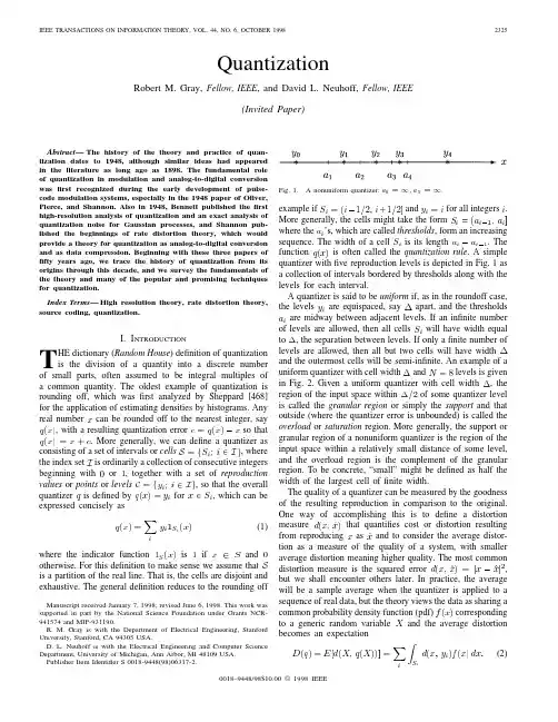
QuantizationRobert M.Gray,Fellow,IEEE,and David L.Neuhoff,Fellow,IEEE(Invited Paper)Abstract—The history of the theory and practice of quan-tization dates to1948,although similar ideas had appearedin the literature as long ago as1898.The fundamental roleof quantization in modulation and analog-to-digital conversionwasfirst recognized during the early development of pulse-code modulation systems,especially in the1948paper of Oliver,Pierce,and Shannon.Also in1948,Bennett published thefirsthigh-resolution analysis of quantization and an exact analysis ofquantization noise for Gaussian processes,and Shannon pub-lished the beginnings of rate distortion theory,which wouldprovide a theory for quantization as analog-to-digital conversionand as data compression.Beginning with these three papers offifty years ago,we trace the history of quantization from itsorigins through this decade,and we survey the fundamentals ofthe theory and many of the popular and promising techniquesfor quantization.Index Terms—High resolution theory,rate distortion theory,source coding,quantization.I.I NTRODUCTIONT HE dictionary(Random House)definition of quantizationis the division of a quantity into a discrete numberof small parts,often assumed to be integral multiples ofa common quantity.The oldest example of quantization isrounding off,which wasfirst analyzed by Sheppard[468]for the application of estimating densities by histograms.Anyreal number,with a resulting quantization error so thatis ordinarily a collection of consecutive integersbeginning with,together with a set of reproductionvalues or points or levelsFig. 2.A uniform quantizer.If the distortion is measured by squarederror,into a binaryrepresentation or channel codeword of the quantizer index possible levels and all of thebinary representations or binary codewords have equal length (a temporary assumption),the binary vectors willneed (or the next largerinteger,,unless explicitly specified otherwise.In summary,the goal of quantization is to encode the data from a source,characterized by its probability density function,into as few bits as possible (i.e.,with low rate)in such a way that a reproduction may be recovered from the bits with as high quality as possible (i.e.,with small average distortion).Clearly,there is a tradeoff between the two primary performance measures:average distortion (or simply distortion ,as we will often abbreviate)and rate.This tradeoff may be quantified as the operational distortion-ratefunction or less.Thatis,or less,which is the inverseofor less.We will also be interested in thebest possible performance among all quantizers.Both as a preview and as an occasional benchmark for comparison,we informally define the class of all quantizers as the class of quantizers that can 1)operate on scalars or vectors instead of only on scalars (vector quantizers),2)have fixed or variable rate in the sense that the binary codeword describing the quantizer output can have length depending on the input,and 3)be memoryless or have memory,for example,using different sets of reproduction levels,depending on the past.In addition,we restrict attention to quantizers that do not change with time.That is,when confronted with the same input and the same past history,a quantizer will produce the same output regardless of the time.We occasionally use the term lossy source code or simply code as alternatives to quantizer .The rate is now defined as the average number of bits per source symbol required to describe the corresponding reproduction symbol.We informally generalize the operational distortion-ratefunctionor less.ThusGRAY AND NEUHOFF:QUANTIZATION2327for special nonasymptotic cases,such as Clavier,Panter, and Grieg’s1947analysis of the spectra of the quantization error for uniformly quantized sinusoidal signals[99],[100], and Bennett’s1948derivation of the power spectral density of a uniformly quantized Gaussian random process[43]. The most important nonasymptotic results,however,are the basic optimality conditions and iterative-descent algorithms for quantizer design,such asfirst developed by Steinhaus(1956) [480]and Lloyd(1957)[330],and later popularized by Max (1960)[349].Our goal in the next section is to introduce in historical context many of the key ideas of quantization that originated in classical works and evolved over the past50years,and in the remaining sections to survey selectively and in more detail a variety of results which illustrate both the historical development and the state of thefield.Section III will present basic background material that will be needed in the remainder of the paper,including the general definition of a quantizer and the basic forms of optimality criteria and descent algorithms. Some such material has already been introduced and more will be introduced in Section II.However,for completeness, Section III will be largely self-contained.Section IV reviews the development of quantization theories and compares the approaches.Finally,Section V describes a number of specific quantization techniques.In any review of a large subject such as quantization there is no space to discuss or even mention all work on the subject. Though we have made an effort to select the most important work,no doubt we have missed some important work due to bias,misunderstanding,or ignorance.For this we apologize, both to the reader and to the researchers whose work we may have neglected.II.H ISTORYThe history of quantization often takes on several parallel paths,which causes some problems in our clustering of topics. We follow roughly a chronological order within each and order the paths as best we can.Specifically,we willfirst track the design and analysis of practical quantization techniques in three paths:fixed-rate scalar quantization,which leads directly from the discussion of Section I,predictive and transform coding,which adds linear processing to scalar quantization in order to exploit source redundancy,and variable-rate quantiza-tion,which uses Shannon’s lossless source coding techniques [464]to reduce rate.(Lossless codes were originally called noiseless.)Next we follow early forward-looking work on vector quantization,including the seminal work of Shannon and Zador,in which vector quantization appears more to be a paradigm for analyzing the fundamental limits of quantizer performance than a practical coding technique.A surprising amount of such vector quantization theory was developed out-side the conventional communications and signal processing literature.Subsequently,we review briefly the developments from the mid-1970’s to the mid-1980’s which mainly concern the emergence of vector quantization as a practical technique. Finally,we sketch briefly developments from the mid-1980’s to the present.Except where stated otherwise,we presume squared error as the distortion measure.A.Fixed-Rate Scalar Quantization:PCM and the Origins of Quantization TheoryBoth quantization and source coding with afidelity crite-rion have their origins in pulse-code modulation(PCM),a technique patented in1938by Reeves[432],who25years later wrote a historical perspective on and an appraisal of the future of PCM with Deloraine[120].The predictions were surprisingly accurate as to the eventual ubiquity of digital speech and video.The technique wasfirst successfully imple-mented in hardware by Black,who reported the principles and implementation in1947[51],as did another Bell Labs paper by Goodall[209].PCM was subsequently analyzed in detail and popularized by Oliver,Pierce,and Shannon in1948[394]. PCM was thefirst digital technique for conveying an analog information signal(principally telephone speech)over an analog channel(typically,a wire or the atmosphere).In other words,it is a modulation technique,i.e.,an alternative to AM, FM,and various other types of pulse modulation.It consists of three main components:a sampler(including a prefilter),a quantizer(with afixed-rate binary encoder),and a binary pulse modulator.The sampler converts a continuous-timewaveform into a sequence ofsamples,whereand the high-frequency power removed by the lowpassfilter.The binary pulse modulator typically uses the bits produced by the quantizer to determine the amplitude,frequency,or phase of a sinusoidal carrier waveform.In the evolutionary development of modulation techniques it was found that the performance of pulse-amplitude modulation in the presence of noise could be improved if the samples were quantized to the nearest of a setoflevels had been transmitted in the presence of noise could be done with such reliability that the overall MSE was substantially reduced.Reducing the number of quantizationlevelsat a value giving acceptably small quantizer MSE and to binary encode the levels,so that the receiver had only to make binary decisions,something it can do with great reliability.The resulting system,PCM,had the best resistance to noise of all modulations of the time.As the digital era emerged,it was recognized that the sampling,quantizing,and encoding part of PCM performs an analog-to-digital(A/D)conversion,with uses extending much beyond communication over analog channels.Even in the communicationsfield,it was recognized that the task of analog-to-digital conversion(and source coding)should be factored out of binary modulation as a separate task.Thus2328IEEE TRANSACTIONS ON INFORMATION THEORY,VOL.44,NO.6,OCTOBER1998 PCM is now generally considered to just consist of sampling,quantizing,and encoding;i.e.,it no longer includes the binarypulse modulation.Although quantization in the information theory literatureis generally considered as a form of data compression,itsuse for modulation or A/D conversion was originally viewedas data expansion or,more accurately,bandwidth expansion.For example,a speech waveform occupying roughly4kHzwould have a Nyquist rate of8kHz.Sampling at the Nyquistrate and quantizing at8bits per sample and then modulatingthe resulting binary pulses using amplitude-or frequency-shiftkeying would yield a signal occupying roughly64kHz,a16–fold increase in bandwidth!Mathematically this constitutescompression in the sense that a continuous waveform requiringan infinite number of bits is reduced to afinite number of bits,but for practical purposes PCM is not well interpreted as acompression scheme.In an early contribution to the theory of quantization,Clavier,Panter,and Grieg(1947)[99],[100]applied Rice’scharacteristic function or transform method[434]to provideexact expressions for the quantization error and its momentsresulting from uniform quantization for certain specific inputs,including constants and sinusoids.The complicated sums ofBessel functions resembled the early analyses of anothernonlinear modulation technique,FM,and left little hope forgeneral closed-form solutions for interesting signals.Thefirst general contributions to quantization theory camein1948with the papers of Oliver,Pierce,and Shannon[394]and Bennett[43].As part of their analysis of PCM forcommunications,they developed the oft-quoted result that forlarge rate or resolution,a uniform quantizer with cellwidthlevels andrate,and the source has inputrange(or support)ofwidthdBshowing that for large rate,the SNR of uniform quantizationincreases6dB for each one-bit increase of rate,which is oftenreferred to as the“6-dB-per-bit rule.”Thefor companders,systems that preceded auniform quantizer by a monotonic smooth nonlinearity calleda“compressor,”saywas givenby is auniform quantizer.Bennett showed that in thiscaseis the cellwidth of the uniformquantizer,and the integral is taken over the granular range ofthe input.(Theconstantmaps to the unit intervalcan be interpreted,as Lloydwould explicitly point out in1957[330],as a constant timesa“quantizer point-densityfunctionnumber of quantizer levelsinover a region gives the fraction ofquantizer reproduction levels in the region,it is evidentthat,which when integratedoverrather than the fraction.In the currentsituationis infinite.Rewriting Bennett’s integral in terms of the point-densityfunction yields its more commonform(7)The idea of a quantizer point-density function will generalizeto vectors,while the compander approach will not in the sensethat not all vector quantizers can be represented as companders[192].Bennett also demonstrated that,under assumptions of highresolution and smooth densities,the quantization error behavedmuch like random“noise”:it had small correlation with thesignal and had approximately aflat(“white”)spectrum.Thisled to an“additive-noise”model of quantizer error,since withthese properties theformulaGRAY AND NEUHOFF:QUANTIZATION2329 is uniformly quantized,providing one of the very few exactcomputations of quantization error spectra.In1951Panter and Dite[405]developed a high-resolutionformula for the distortion of afixed-rate scalar quantizer usingapproximations similar to Bennett’s,but without reference toBennett.They then used variational techniques to minimizetheir formula and found the following formula for the opera-tional distortion-rate function offixed-rate scalar quantization:for large valuesof(9)Indeed,substituting this point density into Bennett’s integraland using the factthat yields(8).As an example,if the input density is Gaussian withvariance,thenasor less.(It was not until Shannon’s1959paper[465]thatthe rate is0.72bits/sample larger thanthat achievable by the best quantizers.In1957,Smith[474]re-examined companding and PCM.Among other things,he gave somewhat cleaner derivations of1They also indicated that it had been derived earlier by P.R.Aigrain.Bennett’s integral,the optimal compressor function,and thePanter–Dite formula.Also in1957,Lloyd[330]made an important study ofquantization with three main contributions.First,he foundnecessary and sufficient conditions for afixed-rate quantizer tobe locally optimal;i.e.,conditions that if satisfied implied thatsmall perturbations to the levels or thresholds would increasedistortion.Any optimal quantizer(one with smallest distortion)will necessarily satisfy these conditions,and so they are oftencalled the optimality conditions or the necessary conditions.Simply stated,Lloyd’s optimality conditions are that for afixed-rate quantizer to be optimal,the quantizer partition mustbe optimal for the set of reproduction levels,and the set ofreproduction levels must be optimal for the partition.Lloydderived these conditions straightforwardly fromfirst principles,without recourse to variational concepts such as derivatives.For the case of mean-squared error,thefirst condition impliesa minimum distance or nearest neighbor quantization rule,choosing the closest available reproduction level to the sourcesample being quantized,and the second condition implies thatthe reproduction level corresponding to a given cell is theconditional expectation or centroid of the source value giventhat it lies in the specified cell;i.e.,it is the minimum mean-squared error estimate of the source sample.For some sourcesthere are multiple locally optimal quantizers,not all of whichare globally optimal.Second,based on his optimality conditions,Lloyd devel-oped an iterative descent algorithm for designing quantizers fora given source distribution:begin with an initial collection ofreproduction levels;optimize the partition for these levels byusing a minimum distortion mapping,which gives a partitionof the real line into intervals;then optimize the set of levels forthe partition by replacing the old levels by the centroids of thepartition cells.The alternation is continued until convergenceto a local,if not global,optimum.Lloyd referred to thisdesign algorithm as“Method I.”He also developed a MethodII based on the optimality properties.First choose an initialsmallest reproduction level.This determines the cell thresholdto the right,which in turn implies the next larger reproductionlevel,and so on.This approach alternately produces a leveland a threshold.Once the last level has been chosen,theinitial level can then be rechosen to reduce distortion andthe algorithm continues.Lloyd provided design examplesfor uniform,Gaussian,and Laplacian random variables andshowed that the results were consistent with the high resolutionapproximations.Although Method II would initially gain morepopularity when rediscovered in1960by Max[349],it isMethod I that easily extends to vector quantizers and manytypes of quantizers with structural constraints.Third,motivated by the work of Panter and Dite butapparently unaware of that of Bennett or Smith,Lloyd re-derived Bennett’s integral and the Panter–Dite formula basedon the concept of point-density function.This was a criticallyimportant step for subsequent generalizations of Bennett’sintegral to vector quantizers.He also showed directly thatin situations where the global optimum is the only localoptimum,quantizers that satisfy the optimality conditionshave,asymptotically,the optimal point density given by(9).2330IEEE TRANSACTIONS ON INFORMATION THEORY,VOL.44,NO.6,OCTOBER1998Unfortunately,Lloyd’s work was not published in an archival journal at the time.Instead,it was presented at the1957Institute of Mathematical Statistics(IMS)meeting and appeared in print only as a Bell Laboratories Technical Memorandum.As a result,its results were not widely known in the engineering literature for many years,and many were independently rediscovered.All of the independent rediscoveries,however,used variational derivations,rather than Lloyd’s simple derivations.The latter were essential for later extensions to vector quantizers and to the development of many quantizer optimization procedures.To our knowledge, thefirst mention of Lloyd’s work in the IEEE literature came in 1964with Fleischer’s[170]derivation of a sufficient condition (namely,that the log of the source density be concave)in order that the optimal quantizer be the only locally optimal quantizer, and consequently,that Lloyd’s Method I yields a globally optimal quantizer.(The condition is satisfied for common densities such as Gaussian and Laplacian.)Zador[561]had referred to Lloyd a year earlier in his Ph.D.dissertation,to be discussed later.Later in the same year in another Bell Telephone Laborato-ries Technical Memorandum,Goldstein[207]used variational methods to derive conditions for global optimality of a scalar quantizer in terms of second-order partial derivatives with respect to the quantizer levels and thresholds.He also provided a simple counterintuitive example of a symmetric density for which the optimal quantizer was asymmetric.In1959,Shtein[471]added terms representing overload distortion totheth-power distortion measures, rediscovered Lloyd’s Method II,and numerically investigated the design offixed-rate quantizers for a variety of input densities.Also in1960,Widrow[529]derived an exact formula for the characteristic function of a uniformly quantized signal when the quantizer has an infinite number of levels.His results showed that under the condition that the characteristic function of the input signal be zero when its argument is greaterthanis a deterministic function of the signal.The“bandlimited”property of the characteristic function implies from Fourier transform theory that the probability density function must have infinite support since a signal and its transform cannot both be perfectly bandlimited.We conclude this subsection by mentioning early work that appeared in the mathematical and statistical literature and which,in hindsight,can be viewed as related to scalar quantization.Specifically,in1950–1951Dalenius et al.[118],[119]used variational techniques to consider optimal group-ing of Gaussian data with respect to average squared error. Lukaszewicz and H.Steinhaus[336](1955)developed what we now consider to be the Lloyd optimality conditions using variational techniques in a study of optimum go/no-go gauge sets(as acknowledged by Lloyd).Cox in1957[111]also derived similar conditions.Some additional early work,which can now be seen as relating to vector quantization,will be reviewed later[480],[159],[561].B.Scalar Quantization with MemoryIt was recognized early that common sources such as speech and images had considerable“redundancy”that scalar quantization could not exploit.The term“redundancy”was commonly used in the early days and is still popular in some of the quantization literature.Strictly speaking,it refers to the statistical correlation or dependence between the samples of such sources and is usually referred to as memory in the information theory literature.As our current emphasis is historical,we follow the traditional language.While not dis-rupting the performance of scalar quantizers,such redundancy could be exploited to attain substantially better rate-distortion performance.The early approaches toward this end combined linear processing with scalar quantization,thereby preserving the simplicity of scalar quantization while using intuition-based arguments and insights to improve performance by incorporating memory into the overall code.The two most important approaches of this variety were predictive coding and transform coding.A shared intuition was that a prepro-cessing operation intended to make scalar quantization more efficient should“remove the redundancy”in the data.Indeed, to this day there is a common belief that data compression is equivalent to redundancy removal and that data without redundancy cannot be further compressed.As will be discussed later,this belief is contradicted both by Shannon’s work, which demonstrated strictly improved performance using vec-tor quantizers even for memoryless sources,and by the early work of Fejes Toth(1959)[159].Nevertheless,removing redundancy leads to much improved codes.Predictive quantization appears to originate in the1946 delta modulation patent of Derjavitch,Deloraine,and Van Mierlo[129],but the most commonly cited early references are Cutler’s patent[117]2605361on“Differential quantization of communication signals”and on DeJager’s Philips technical report on delta modulation[128].Cutler stated in his patent that it“is the object of the present invention to improve the efficiency of communication systems by taking advantage of correlation in the signals of these systems”and Derjavitch et al.also cited the reduction of redundancy as the key to the re-duction of quantization noise.In1950,Elias[141]provided an information-theoretic development of the benefits of predictive coding,but the work was not published until1955[142].Other early references include[395],[300],[237],[511],and[572]. In particular,[511]claims Bennett-style asymptotics for high-resolution quantization error,but as will be discussed later, such approximations have yet to be rigorously derived. From the point of view of least squares estimation theory,if one were to optimally predict a data sequence based on its pastGRAY AND NEUHOFF:QUANTIZATION2331Fig.3.Predictive quantizer encoder/decoder.in the sense of minimizing the mean-squared error,then the resulting error or residual or innovations sequence would be uncorrelated and it would have the minimum possible variance. To permit reconstruction in a coded system,however,the prediction must be based on past reconstructed samples and not true samples.This is accomplished by placing a quantizer inside a prediction loop and using the same predictor to decode the signal.A simple predictive quantizer or differential pulse-coded modulator(DPCM)is depicted in Fig.3.If the predictor is simply the last sample and the quantizer has only one bit, the system becomes a delta-modulator.Predictive quantizers are considered to have memory in that the quantization of a sample depends on previous samples,via the feedback loop. Predictive quantizers have been extensively developed,for example there are many adaptive versions,and are widely used in speech and video coding,where a number of standards are based on them.In speech coding they form the basis of ITU-G.721,722,723,and726,and in video coding they form the basis of the interframe coding schemes standardized in the MPEG and H.26X prehensive discussions may be found in books[265],[374],[196],[424],[50],and[458],as well as survey papers[264]and[198].Though decorrelation was an early motivation for predictive quantization,the most common view at present is that the primary role of the predictor is to reduce the variance of the variable to be scalar-quantized.This view stems from the facts that a)it is the prediction errors rather than the source samples that are quantized,b)the overall quantization error precisely equals that of the scalar quantizer operating on the prediction errors,c)the operational distortion-ratefunctionresults in a scalingof,where is the variance of the sourceandthat is multiplied by an orthogonal matrix(an2332IEEE TRANSACTIONS ON INFORMATION THEORY,VOL.44,NO.6,OCTOBER1998Fig.4.Transform code.orthogonal transform)and the resulting transform coefficients are scalar quantized,usually with a different quantizer for each coefficient.The operation is depicted in Fig.4.This style of code was introduced in1956by Kramer and Mathews [299]and analyzed and popularized in1962–1963by Huang and Schultheiss[247],[248].Kramer and Mathews simply assumed that the goal of the transform was to decorrelate the symbols,but Huang and Schultheiss proved that decorrelating does indeed lead to optimal transform code design,at least in the case of Gaussian sources and high resolution.Transform coding has been extensively developed for coding images and video,where the discrete cosine transform(DCT)[7], [429]is most commonly used because of its computational simplicity and its good performance.Indeed,DCT coding is the basic approach dominating current image and video coding standards,including H.261,H.263,JPEG,and MPEG.These codes combine uniform scalar quantization of the transform coefficients with an efficient lossless coding of the quantizer indices,as will be considered in the next section as a variable-rate quantizer.For discussions of transform coding for images see[533],[422],[375],[265],[98],[374],[261],[424],[196], [208],[408],[50],[458],and More recently,transform coding has also been widely used in high-fidelity audio coding[272], [200].Unlike predictive quantizers,the transform coding approach lent itself quite well to the Bennett high-resolution approx-imations,the classical analysis being that of Huang and Schultheiss[247],[248]of the performance of optimized transform codes forfixed-rate scalar quantizers for Gaussian sources,a result which demonstrated that the Karhunen–Lo`e ve decorrelating transform was optimum for this application for the given assumptions.If the transform is the Karhunen–Lo`e ve transform,then the coefficients will be uncorrelated(and hence independent if the input vector is also Gaussian).The seminal work of Huang and Schultheiss showed that high-resolution approximation theory could provide analytical descriptions of optimal performance and design algorithms for optimizing codes of a given structure.In particular,they showed that under the high-resolution assumptions with Gaussian sources, the average distortion of the best transform code with a given rate is less than that of optimal scalar quantization bythefactor,where is the average of thevariances of the components of the source vectorandcovariance matrix.Note that this reduction indistortion becomes larger for sources with more memory(morecorrelation)because the covariance matrices of such sourceshave smaller determinants.Whenor less.Sincewe have weakened the constraint by expanding the allowedset of quantizers,this operational distortion-rate function willordinarily be smaller than thefixed-rate optimum.Huffman’s algorithm[251]provides a systematic methodof designing binary codes with the smallest possible averagelength for a given set of probabilities,such as those of thecells.Codes designed in this way are typically called Huffmancodes.Unfortunately,there is no known expression for theresulting minimum average length in terms of the probabilities.However,Shannon’s lossless source coding theorem impliesthat given a source and a quantizer partition,one can alwaysfind an assignment of binary codewords(indeed,a prefix set)with average length not morethan,where。

The Paradigm Advantage+ Full-azimuth angle domain imaging and analysis maximizes knowledge from seismic data.+ Maximized ROI for deep water, unconventional shale resource plays and fractured carbonate reservoirs.+ Extracts unprecedented value from all modern and legacy seismic data acquisitions, notably those with wide and rich azimuth and long offset.+ Delivers highly accurate isotropic/anisotropic velocity models, especially in complex subsurface areas.+ Delivers high-resolution information about principal reservoir properties.+ Extends the capabilities of leading Paradigm processing, imaging and analysis systems.EarthStudy 360 ®Full-Azimuth Angle Domain Imaging and AnalysisInteroperabilityAll Epos-based applications enable interoperability with third-party data stores, including:- OpenWorks ® 2003.12, R-5000 - GeoFrame ® 4.5 - OpenSpirit ® 3System specifications- All 64-bit, for x64 architecture processors- Red Hat ® Enterprise Linux ® 5.3 and above, 6.0 and aboveIllumination for Seismic Data MiningThe EarthStudy 360 Illuminator is an advanced seismic data mining tool that provides a previously unattainable breadth of knowledge about ray propagation in complex areas.The Illuminator uses an enhanced, interactive ray tracing technology that both quantifies and qualifies the relationship between the surface acquisition geometry and the subsurface angles in targeted areas. Launched from the Paradigm SeisEarth ®or GeoDepth ®3D Canvas,input for the Illuminator includes isotropic/anisotropic velocity models and optionally, data acquisition geometry. Interpreters can generate ray attributes, illumination and reliability maps to gain knowledge about the quality and integrity of the seismic image. A user who wants to know more about why certain areas have low reliability, has access to an extensive set of tools which deliverthat knowledge. The results are displayed in a clear visual manner, simplifying even the most complex set of imaging characteristics.In addition to all the functionalities of the Illuminator, EarthStudy 360 Illuminator Plus can perform ray tracing in batch mode along fine 3D grids for the generation of full-azimuth illumination and ray attribute gathers, volumes and maps. Grid-based ray tracing is supported by Paradigm’s HPC functionality and can run on multi-node clusters. Illuminator Plus is aimed at depthInteractive ray tracing as a tool for understanding quality of common image gather eventsTwo-point ray tracing in complex subsurfaceimaging specialists who seek additional knowledge about imaging reliability.Enhancing Velocity Modeling and Amplitude InversionEarthStudy 360 significantly extends the velocity modeling capabilities of Paradigm’s industry-leading GeoDepth imaging and velocity determination system. Theinformation gained from the 3D angle gathers provides the seismic imaging specialist with additional knowledge about the subsurface, enabling a more accurate and reliable velocity model. Similarly, for the geoscientist using the Probe ® AVO/AVA system to analyze amplitude variation with angle and azimuth (AVAZ), the rich information obtained from all angles and azimuths enhances accuracy and reduces uncertainty in hydrocarbon detection, fracture detection, and other reservoir properties that are vital to the exploration and production work cycle.3D illumination angle gatherProcessing and ImagingDirectional and Reflection Angle Gather SystemsEarthStudy 360 enables geophysicists to use all recorded seismic data in a continuous fashion directly in the subsurface local angle domain. This results in two complementary, full-azimuth, 3D angle gather systems: Directional and reflection .Directional angle decomposition implements both specular and diffraction imaging with real 3D isotropic/anisotropic geological models, leading to simultaneous emphasis on both continuous structural surfaces and discontinuous objects such as small faultsEarthStudy 360A new world of information for geoscientistsAdded Value for GeoscientistsEarthStudy 360 creates a wealth of seismic image data, decomposed into full-azimuth, angle-dependent reflection and directional (dip and azimuth) data components. These can be selectively sampled, creatively combined, dynamically visualized, and further processed to secure images of the subsurface. The images can reveal the information needed for velocity model determination, as well as provide details regarding the presence of micro-fractures, the orientation of faults and fractures, the influence of anisotropy, the directions of contributing illumination, the elastic properties of target reservoirs, and the boundaries of those reservoirs .New Technologies for a New AgeDeclining production in mature oil and gas fields is forcing upstream energy companies to explore areas of increasing operational and technical complexity. Existing solutions for extracting information about the subsurface geological model are limited, and there is a need to expand current technologies to include the acquisition of wide and rich azimuth seismic data. Paradigm is the first to meet this need with EarthStudy 360, a new invention designed to image, characterize, visualize and interpret the total seismic wavefield.Expanding the Frontiers of Subsurface ExplorationParadigm ™ EarthStudy 360® is an innovative new system designed to deliver to both depth imaging experts and interpretation specialists a complete set of data that enables them to obtain accurate subsurface velocity models, structural attributes, medium properties and reservoir characteristics. The system extracts unprecedented value from all modern and legacy seismic data acquisitions, especially those with wide and rich azimuth and long offset, in both marine and land environments. EarthStudy 360 is most effective for imaging and analysis in unconventional gas plays within shale formations and in fracture carbonate reservoirs. The system delivers highly accurate images from below complex structures such as shallow low-velocity anomalies like gas pockets, subsalt, sub-basalt and high-velocity carbonate rocks. These result in optimal solutions for anisotropic tomography and for fracture detection and reservoir characterization.Directional angle gather near geologic pinchout: Two specular signature directions at same locationHidden structure revealed by EarthStudy 360。

Modeling the Spatial Dynamics of Regional Land Use:The CLUE-S ModelPETER H.VERBURG*Department of Environmental Sciences Wageningen UniversityP.O.Box376700AA Wageningen,The NetherlandsandFaculty of Geographical SciencesUtrecht UniversityP.O.Box801153508TC Utrecht,The NetherlandsWELMOED SOEPBOERA.VELDKAMPDepartment of Environmental Sciences Wageningen UniversityP.O.Box376700AA Wageningen,The NetherlandsRAMIL LIMPIADAVICTORIA ESPALDONSchool of Environmental Science and Management University of the Philippines Los Ban˜osCollege,Laguna4031,Philippines SHARIFAH S.A.MASTURADepartment of GeographyUniversiti Kebangsaan Malaysia43600BangiSelangor,MalaysiaABSTRACT/Land-use change models are important tools for integrated environmental management.Through scenario analysis they can help to identify near-future critical locations in the face of environmental change.A dynamic,spatially ex-plicit,land-use change model is presented for the regional scale:CLUE-S.The model is specifically developed for the analysis of land use in small regions(e.g.,a watershed or province)at afine spatial resolution.The model structure is based on systems theory to allow the integrated analysis of land-use change in relation to socio-economic and biophysi-cal driving factors.The model explicitly addresses the hierar-chical organization of land use systems,spatial connectivity between locations and stability.Stability is incorporated by a set of variables that define the relative elasticity of the actual land-use type to conversion.The user can specify these set-tings based on expert knowledge or survey data.Two appli-cations of the model in the Philippines and Malaysia are used to illustrate the functioning of the model and its validation.Land-use change is central to environmental man-agement through its influence on biodiversity,water and radiation budgets,trace gas emissions,carbon cy-cling,and livelihoods(Lambin and others2000a, Turner1994).Land-use planning attempts to influence the land-use change dynamics so that land-use config-urations are achieved that balance environmental and stakeholder needs.Environmental management and land-use planning therefore need information about the dynamics of land use.Models can help to understand these dynamics and project near future land-use trajectories in order to target management decisions(Schoonenboom1995).Environmental management,and land-use planning specifically,take place at different spatial and organisa-tional levels,often corresponding with either eco-re-gional or administrative units,such as the national or provincial level.The information needed and the man-agement decisions made are different for the different levels of analysis.At the national level it is often suffi-cient to identify regions that qualify as“hot-spots”of land-use change,i.e.,areas that are likely to be faced with rapid land use conversions.Once these hot-spots are identified a more detailed land use change analysis is often needed at the regional level.At the regional level,the effects of land-use change on natural resources can be determined by a combina-tion of land use change analysis and specific models to assess the impact on natural resources.Examples of this type of model are water balance models(Schulze 2000),nutrient balance models(Priess and Koning 2001,Smaling and Fresco1993)and erosion/sedimen-tation models(Schoorl and Veldkamp2000).Most of-KEY WORDS:Land-use change;Modeling;Systems approach;Sce-nario analysis;Natural resources management*Author to whom correspondence should be addressed;email:pverburg@gissrv.iend.wau.nlDOI:10.1007/s00267-002-2630-x Environmental Management Vol.30,No.3,pp.391–405©2002Springer-Verlag New York Inc.ten these models need high-resolution data for land use to appropriately simulate the processes involved.Land-Use Change ModelsThe rising awareness of the need for spatially-ex-plicit land-use models within the Land-Use and Land-Cover Change research community(LUCC;Lambin and others2000a,Turner and others1995)has led to the development of a wide range of land-use change models.Whereas most models were originally devel-oped for deforestation(reviews by Kaimowitz and An-gelsen1998,Lambin1997)more recent efforts also address other land use conversions such as urbaniza-tion and agricultural intensification(Brown and others 2000,Engelen and others1995,Hilferink and Rietveld 1999,Lambin and others2000b).Spatially explicit ap-proaches are often based on cellular automata that simulate land use change as a function of land use in the neighborhood and a set of user-specified relations with driving factors(Balzter and others1998,Candau 2000,Engelen and others1995,Wu1998).The speci-fication of the neighborhood functions and transition rules is done either based on the user’s expert knowl-edge,which can be a problematic process due to a lack of quantitative understanding,or on empirical rela-tions between land use and driving factors(e.g.,Pi-janowski and others2000,Pontius and others2000).A probability surface,based on either logistic regression or neural network analysis of historic conversions,is made for future conversions.Projections of change are based on applying a cut-off value to this probability sur-face.Although appropriate for short-term projections,if the trend in land-use change continues,this methodology is incapable of projecting changes when the demands for different land-use types change,leading to a discontinua-tion of the trends.Moreover,these models are usually capable of simulating the conversion of one land-use type only(e.g.deforestation)because they do not address competition between land-use types explicitly.The CLUE Modeling FrameworkThe Conversion of Land Use and its Effects(CLUE) modeling framework(Veldkamp and Fresco1996,Ver-burg and others1999a)was developed to simulate land-use change using empirically quantified relations be-tween land use and its driving factors in combination with dynamic modeling.In contrast to most empirical models,it is possible to simulate multiple land-use types simultaneously through the dynamic simulation of competition between land-use types.This model was developed for the national and con-tinental level,applications are available for Central America(Kok and Winograd2001),Ecuador(de Kon-ing and others1999),China(Verburg and others 2000),and Java,Indonesia(Verburg and others 1999b).For study areas with such a large extent the spatial resolution of analysis was coarse(pixel size vary-ing between7ϫ7and32ϫ32km).This is a conse-quence of the impossibility to acquire data for land use and all driving factors atfiner spatial resolutions.A coarse spatial resolution requires a different data rep-resentation than the common representation for data with afine spatial resolution.Infine resolution grid-based approaches land use is defined by the most dom-inant land-use type within the pixel.However,such a data representation would lead to large biases in the land-use distribution as some class proportions will di-minish and other will increase with scale depending on the spatial and probability distributions of the cover types(Moody and Woodcock1994).In the applications of the CLUE model at the national or continental level we have,therefore,represented land use by designating the relative cover of each land-use type in each pixel, e.g.a pixel can contain30%cultivated land,40%grass-land,and30%forest.This data representation is di-rectly related to the information contained in the cen-sus data that underlie the applications.For each administrative unit,census data denote the number of hectares devoted to different land-use types.When studying areas with a relatively small spatial ex-tent,we often base our land-use data on land-use maps or remote sensing images that denote land-use types respec-tively by homogeneous polygons or classified pixels. When converted to a raster format this results in only one, dominant,land-use type occupying one unit of analysis. The validity of this data representation depends on the patchiness of the landscape and the pixel size chosen. Most sub-national land use studies use this representation of land use with pixel sizes varying between a few meters up to about1ϫ1km.The two different data represen-tations are shown in Figure1.Because of the differences in data representation and other features that are typical for regional appli-cations,the CLUE model can not directly be applied at the regional scale.This paper describes the mod-ified modeling approach for regional applications of the model,now called CLUE-S(the Conversion of Land Use and its Effects at Small regional extent). The next section describes the theories underlying the development of the model after which it is de-scribed how these concepts are incorporated in the simulation model.The functioning of the model is illustrated for two case-studies and is followed by a general discussion.392P.H.Verburg and othersCharacteristics of Land-Use SystemsThis section lists the main concepts and theories that are prevalent for describing the dynamics of land-use change being relevant for the development of land-use change models.Land-use systems are complex and operate at the interface of multiple social and ecological systems.The similarities between land use,social,and ecological systems allow us to use concepts that have proven to be useful for studying and simulating ecological systems in our analysis of land-use change (Loucks 1977,Adger 1999,Holling and Sanderson 1996).Among those con-cepts,connectivity is important.The concept of con-nectivity acknowledges that locations that are at a cer-tain distance are related to each other (Green 1994).Connectivity can be a direct result of biophysical pro-cesses,e.g.,sedimentation in the lowlands is a direct result of erosion in the uplands,but more often it is due to the movement of species or humans through the nd degradation at a certain location will trigger farmers to clear land at a new location.Thus,changes in land use at this new location are related to the land-use conditions in the other location.In other instances more complex relations exist that are rooted in the social and economic organization of the system.The hierarchical structure of social organization causes some lower level processes to be constrained by higher level dynamics,e.g.,the establishments of a new fruit-tree plantation in an area near to the market might in fluence prices in such a way that it is no longer pro fitable for farmers to produce fruits in more distant areas.For studying this situation an-other concept from ecology,hierarchy theory,is use-ful (Allen and Starr 1982,O ’Neill and others 1986).This theory states that higher level processes con-strain lower level processes whereas the higher level processes might emerge from lower level dynamics.This makes the analysis of the land-use system at different levels of analysis necessary.Connectivity implies that we cannot understand land use at a certain location by solely studying the site characteristics of that location.The situation atneigh-Figure 1.Data representation and land-use model used for respectively case-studies with a national/continental extent and local/regional extent.Modeling Regional Land-Use Change393boring or even more distant locations can be as impor-tant as the conditions at the location itself.Land-use and land-cover change are the result of many interacting processes.Each of these processes operates over a range of scales in space and time.These processes are driven by one or more of these variables that influence the actions of the agents of land-use and cover change involved.These variables are often re-ferred to as underlying driving forces which underpin the proximate causes of land-use change,such as wood extraction or agricultural expansion(Geist and Lambin 2001).These driving factors include demographic fac-tors(e.g.,population pressure),economic factors(e.g., economic growth),technological factors,policy and institutional factors,cultural factors,and biophysical factors(Turner and others1995,Kaimowitz and An-gelsen1998).These factors influence land-use change in different ways.Some of these factors directly influ-ence the rate and quantity of land-use change,e.g.the amount of forest cleared by new incoming migrants. Other factors determine the location of land-use change,e.g.the suitability of the soils for agricultural land use.Especially the biophysical factors do pose constraints to land-use change at certain locations, leading to spatially differentiated pathways of change.It is not possible to classify all factors in groups that either influence the rate or location of land-use change.In some cases the same driving factor has both an influ-ence on the quantity of land-use change as well as on the location of land-use change.Population pressure is often an important driving factor of land-use conver-sions(Rudel and Roper1997).At the same time it is the relative population pressure that determines which land-use changes are taking place at a certain location. Intensively cultivated arable lands are commonly situ-ated at a limited distance from the villages while more extensively managed grasslands are often found at a larger distance from population concentrations,a rela-tion that can be explained by labor intensity,transport costs,and the quality of the products(Von Thu¨nen 1966).The determination of the driving factors of land use changes is often problematic and an issue of dis-cussion(Lambin and others2001).There is no unify-ing theory that includes all processes relevant to land-use change.Reviews of case studies show that it is not possible to simply relate land-use change to population growth,poverty,and infrastructure.Rather,the inter-play of several proximate as well as underlying factors drive land-use change in a synergetic way with large variations caused by location specific conditions (Lambin and others2001,Geist and Lambin2001).In regional modeling we often need to rely on poor data describing this complexity.Instead of using the under-lying driving factors it is needed to use proximate vari-ables that can represent the underlying driving factors. Especially for factors that are important in determining the location of change it is essential that the factor can be mapped quantitatively,representing its spatial vari-ation.The causality between the underlying driving factors and the(proximate)factors used in modeling (in this paper,also referred to as“driving factors”) should be certified.Other system properties that are relevant for land-use systems are stability and resilience,concepts often used to describe ecological systems and,to some extent, social systems(Adger2000,Holling1973,Levin and others1998).Resilience refers to the buffer capacity or the ability of the ecosystem or society to absorb pertur-bations,or the magnitude of disturbance that can be absorbed before a system changes its structure by changing the variables and processes that control be-havior(Holling1992).Stability and resilience are con-cepts that can also be used to describe the dynamics of land-use systems,that inherit these characteristics from both ecological and social systems.Due to stability and resilience of the system disturbances and external in-fluences will,mostly,not directly change the landscape structure(Conway1985).After a natural disaster lands might be abandoned and the population might tempo-rally migrate.However,people will in most cases return after some time and continue land-use management practices as before,recovering the land-use structure (Kok and others2002).Stability in the land-use struc-ture is also a result of the social,economic,and insti-tutional structure.Instead of a direct change in the land-use structure upon a fall in prices of a certain product,farmers will wait a few years,depending on the investments made,before they change their cropping system.These characteristics of land-use systems provide a number requirements for the modelling of land-use change that have been used in the development of the CLUE-S model,including:●Models should not analyze land use at a single scale,but rather include multiple,interconnected spatial scales because of the hierarchical organization of land-use systems.●Special attention should be given to the drivingfactors of land-use change,distinguishing drivers that determine the quantity of change from drivers of the location of change.●Sudden changes in driving factors should not di-rectly change the structure of the land-use system asa consequence of the resilience and stability of theland-use system.394P.H.Verburg and others●The model structure should allow spatial interac-tions between locations and feedbacks from higher levels of organization.Model DescriptionModel StructureThe model is sub-divided into two distinct modules,namely a non-spatial demand module and a spatially explicit allocation procedure (Figure 2).The non-spa-tial module calculates the area change for all land-use types at the aggregate level.Within the second part of the model these demands are translated into land-use changes at different locations within the study region using a raster-based system.For the land-use demand module,different alterna-tive model speci fications are possible,ranging from simple trend extrapolations to complex economic mod-els.The choice for a speci fic model is very much de-pendent on the nature of the most important land-use conversions taking place within the study area and the scenarios that need to be considered.Therefore,the demand calculations will differ between applications and scenarios and need to be decided by the user for the speci fic situation.The results from the demandmodule need to specify,on a yearly basis,the area covered by the different land-use types,which is a direct input for the allocation module.The rest of this paper focuses on the procedure to allocate these demands to land-use conversions at speci fic locations within the study area.The allocation is based upon a combination of em-pirical,spatial analysis,and dynamic modelling.Figure 3gives an overview of the procedure.The empirical analysis unravels the relations between the spatial dis-tribution of land use and a series of factors that are drivers and constraints of land use.The results of this empirical analysis are used within the model when sim-ulating the competition between land-use types for a speci fic location.In addition,a set of decision rules is speci fied by the user to restrict the conversions that can take place based on the actual land-use pattern.The different components of the procedure are now dis-cussed in more detail.Spatial AnalysisThe pattern of land use,as it can be observed from an airplane window or through remotely sensed im-ages,reveals the spatial organization of land use in relation to the underlying biophysical andsocio-eco-Figure 2.Overview of the modelingprocedure.Figure 3.Schematic represen-tation of the procedure to allo-cate changes in land use to a raster based map.Modeling Regional Land-Use Change395nomic conditions.These observations can be formal-ized by overlaying this land-use pattern with maps de-picting the variability in biophysical and socio-economic conditions.Geographical Information Systems(GIS)are used to process all spatial data and convert these into a regular grid.Apart from land use, data are gathered that represent the assumed driving forces of land use in the study area.The list of assumed driving forces is based on prevalent theories on driving factors of land-use change(Lambin and others2001, Kaimowitz and Angelsen1998,Turner and others 1993)and knowledge of the conditions in the study area.Data can originate from remote sensing(e.g., land use),secondary statistics(e.g.,population distri-bution),maps(e.g.,soil),and other sources.To allow a straightforward analysis,the data are converted into a grid based system with a cell size that depends on the resolution of the available data.This often involves the aggregation of one or more layers of thematic data,e.g. it does not make sense to use a30-m resolution if that is available for land-use data only,while the digital elevation model has a resolution of500m.Therefore, all data are aggregated to the same resolution that best represents the quality and resolution of the data.The relations between land use and its driving fac-tors are thereafter evaluated using stepwise logistic re-gression.Logistic regression is an often used method-ology in land-use change research(Geoghegan and others2001,Serneels and Lambin2001).In this study we use logistic regression to indicate the probability of a certain grid cell to be devoted to a land-use type given a set of driving factors following:LogͩP i1ϪP i ͪϭ␤0ϩ␤1X1,iϩ␤2X2,i......ϩ␤n X n,iwhere P i is the probability of a grid cell for the occur-rence of the considered land-use type and the X’s are the driving factors.The stepwise procedure is used to help us select the relevant driving factors from a larger set of factors that are assumed to influence the land-use pattern.Variables that have no significant contribution to the explanation of the land-use pattern are excluded from thefinal regression equation.Where in ordinal least squares regression the R2 gives a measure of modelfit,there is no equivalent for logistic regression.Instead,the goodness offit can be evaluated with the ROC method(Pontius and Schnei-der2000,Swets1986)which evaluates the predicted probabilities by comparing them with the observed val-ues over the whole domain of predicted probabilities instead of only evaluating the percentage of correctly classified observations at afixed cut-off value.This is an appropriate methodology for our application,because we will use a wide range of probabilities within the model calculations.The influence of spatial autocorrelation on the re-gression results can be minimized by only performing the regression on a random sample of pixels at a certain minimum distance from one another.Such a selection method is adopted in order to maximize the distance between the selected pixels to attenuate the problem associated with spatial autocorrelation.For case-studies where autocorrelation has an important influence on the land-use structure it is possible to further exploit it by incorporating an autoregressive term in the regres-sion equation(Overmars and others2002).Based upon the regression results a probability map can be calculated for each land-use type.A new probabil-ity map is calculated every year with updated values for the driving factors that are projected to change in time,such as the population distribution or accessibility.Decision RulesLand-use type or location specific decision rules can be specified by the user.Location specific decision rules include the delineation of protected areas such as nature reserves.If a protected area is specified,no changes are allowed within this area.For each land-use type decision rules determine the conditions under which the land-use type is allowed to change in the next time step.These decision rules are implemented to give certain land-use types a certain resistance to change in order to generate the stability in the land-use structure that is typical for many landscapes.Three different situations can be distinguished and for each land-use type the user should specify which situation is most relevant for that land-use type:1.For some land-use types it is very unlikely that theyare converted into another land-use type after their first conversion;as soon as an agricultural area is urbanized it is not expected to return to agriculture or to be converted into forest cover.Unless a de-crease in area demand for this land-use type occurs the locations covered by this land use are no longer evaluated for potential land-use changes.If this situation is selected it also holds that if the demand for this land-use type decreases,there is no possi-bility for expansion in other areas.In other words, when this setting is applied to forest cover and deforestation needs to be allocated,it is impossible to reforest other areas at the same time.2.Other land-use types are converted more easily.Aswidden agriculture system is most likely to be con-verted into another land-use type soon after its396P.H.Verburg and othersinitial conversion.When this situation is selected for a land-use type no restrictions to change are considered in the allocation module.3.There is also a number of land-use types that oper-ate in between these two extremes.Permanent ag-riculture and plantations require an investment for their establishment.It is therefore not very likely that they will be converted very soon after into another land-use type.However,in the end,when another land-use type becomes more pro fitable,a conversion is possible.This situation is dealt with by de fining the relative elasticity for change (ELAS u )for the land-use type into any other land use type.The relative elasticity ranges between 0(similar to Situation 2)and 1(similar to Situation 1).The higher the de fined elasticity,the more dif ficult it gets to convert this land-use type.The elasticity should be de fined based on the user ’s knowledge of the situation,but can also be tuned during the calibration of the petition and Actual Allocation of Change Allocation of land-use change is made in an iterative procedure given the probability maps,the decision rules in combination with the actual land-use map,and the demand for the different land-use types (Figure 4).The following steps are followed in the calculation:1.The first step includes the determination of all grid cells that are allowed to change.Grid cells that are either part of a protected area or under a land-use type that is not allowed to change (Situation 1,above)are excluded from further calculation.2.For each grid cell i the total probability (TPROP i,u )is calculated for each of the land-use types u accord-ing to:TPROP i,u ϭP i,u ϩELAS u ϩITER u ,where ITER u is an iteration variable that is speci fic to the land use.ELAS u is the relative elasticity for change speci fied in the decision rules (Situation 3de-scribed above)and is only given a value if grid-cell i is already under land use type u in the year considered.ELAS u equals zero if all changes are allowed (Situation 2).3.A preliminary allocation is made with an equalvalue of the iteration variable (ITER u )for all land-use types by allocating the land-use type with the highest total probability for the considered grid cell.This will cause a number of grid cells to change land use.4.The total allocated area of each land use is nowcompared to the demand.For land-use types where the allocated area is smaller than the demanded area the value of the iteration variable is increased.For land-use types for which too much is allocated the value is decreased.5.Steps 2to 4are repeated as long as the demandsare not correctly allocated.When allocation equals demand the final map is saved and the calculations can continue for the next yearly timestep.Figure 5shows the development of the iteration parameter ITER u for different land-use types during asimulation.Figure 4.Representation of the iterative procedure for land-use changeallocation.Figure 5.Change in the iteration parameter (ITER u )during the simulation within one time-step.The different lines rep-resent the iteration parameter for different land-use types.The parameter is changed for all land-use types synchronously until the allocated land use equals the demand.Modeling Regional Land-Use Change397Multi-Scale CharacteristicsOne of the requirements for land-use change mod-els are multi-scale characteristics.The above described model structure incorporates different types of scale interactions.Within the iterative procedure there is a continuous interaction between macro-scale demands and local land-use suitability as determined by the re-gression equations.When the demand changes,the iterative procedure will cause the land-use types for which demand increased to have a higher competitive capacity (higher value for ITER u )to ensure enough allocation of this land-use type.Instead of only being determined by the local conditions,captured by the logistic regressions,it is also the regional demand that affects the actually allocated changes.This allows the model to “overrule ”the local suitability,it is not always the land-use type with the highest probability according to the logistic regression equation (P i,u )that the grid cell is allocated to.Apart from these two distinct levels of analysis there are also driving forces that operate over a certain dis-tance instead of being locally important.Applying a neighborhood function that is able to represent the regional in fluence of the data incorporates this type of variable.Population pressure is an example of such a variable:often the in fluence of population acts over a certain distance.Therefore,it is not the exact location of peoples houses that determines the land-use pattern.The average population density over a larger area is often a more appropriate variable.Such a population density surface can be created by a neighborhood func-tion using detailed spatial data.The data generated this way can be included in the spatial analysis as anotherindependent factor.In the application of the model in the Philippines,described hereafter,we applied a 5ϫ5focal filter to the population map to generate a map representing the general population pressure.Instead of using these variables,generated by neighborhood analysis,it is also possible to use the more advanced technique of multi-level statistics (Goldstein 1995),which enable a model to include higher-level variables in a straightforward manner within the regression equa-tion (Polsky and Easterling 2001).Application of the ModelIn this paper,two examples of applications of the model are provided to illustrate its function.TheseTable nd-use classes and driving factors evaluated for Sibuyan IslandLand-use classes Driving factors (location)Forest Altitude (m)GrasslandSlope Coconut plantation AspectRice fieldsDistance to town Others (incl.mangrove and settlements)Distance to stream Distance to road Distance to coast Distance to port Erosion vulnerability GeologyPopulation density(neighborhood 5ϫ5)Figure 6.Location of the case-study areas.398P.H.Verburg and others。

Unit 14Scheme layout 规划方案traffic schemes交通计划AONB（areas of outstanding natural beauty）著名的自然风景区SSSI（special scientific interest）特殊的科研用地listed buildings 受保护的建筑archaeological sites 考古遗址adherence to 忠诚，坚持turning characteristics 转向性能be recovered from 通过。

的补偿HGV重型货车kerb lines路缘石，路缘线swept paths 加宽车道DoT交通运输部rigid or articulated 刚性的或铰接的车front and rear overhang 前悬和后悬swept area 扫略面积on the major route 主路on the side road 支路channelised layout 渠化方案pelican crossings on the far side 在远处rural 乡下的generous 慷慨的，大方的，有雅量的constraint 约束，强制，局促conservatian 保存，保持，守恒collision 碰撞，冲突condition 条件，情形reroute 变更旅程characteristic 特有的，特征，特性predominate 掌握统治主要的突出口有力的private car 私人汽车manoeuvre 策略调动demountable 可卸下的street furniture 街道家具drawbar 列车间的挂钩wheelbase 轴距车轮接地面积crossroad 十字路十字路口歧途Traffic Planning Steps交通规划步骤（Data collection数据收集Forecasts预测Goal specification明确目标Preparation of alternative plans可选择计划的准备Testing检验Evaluation 评价Implementation实施）Levels（Policy planning政策规划Systems planning系统规划Preliminary engineering初步设施建造Engineering design 建造设计Planning for operations of existing systems or services现存系统运营的设计）Cost estimation 成本估算traffic flow simulation交通流模拟an action plan实施性规划quantitative data数据资料in the light of 按照，根据，当作stratification 层化成层阶层的形成assign 分配指派赋值quantitative 数量的量的transportation improvement 交通运输改善feedback 回授反馈反应deliberate 深思熟虑的故意的null 无效力的，无效的benchmark 基准legislature 立法机关takeover 接收接管transit system 运输系统Conrail 联合铁路公司corridor study 路廊环境研究，高速通道研究deregulation 违反规定Unit 16Four-step planning procedure四阶段规划法：trip generation 出行生成，trip distribution, 出行分布modal split,方式划分traffic assignment交通分配urban transportation planning 城市运输规划transportation facility 运输设施gap 间隙差距Trip rate出行率the target planning years目标规划年trip end 出行端点traffic zone交通小区car trips and public transport trips小汽车和公共交通出行gravity model重力模型centroids traffic zones交通小区形心all-or-nothing assignment 全有全无分配法capacity restrained assignment容量限制分配法multipath proportional assignment多路径概率分配法a measure ofLink impedance路径阻抗interlocking 联锁的favorable 赞成的Unit 17longitudinal spacing纵向间距level terrain 平原地形Rolling terrain丘陵区Mountainous terrain山岭区Crawl speed is the maximum sustained speed that heavy vehicles can maintain on an extended upgrade of a given percent 爬坡速度是重型车辆在一定比例的延长的爬坡段上的最大行驶速度signalization conditions信号控制条件signal phasing信号相位timing配时type of control 控制类型an evaluation of signal progression for each lane group每车道组的信号联动评价的全部规定saturation flow饱和流量saturation flow rate 饱和流率topography 地形学curb 路边account for 说明解决得分estimation 估计，预算，评价Unit 18fatalities.恶性事故motorcycle occupant摩托车成员vehicle-miles traveled车公里poorly timed signals配时不当House of Representatives' Subcommittee众议院Federal aid Highways hearings联邦政府助建公路Unit 19Biographical descriptors个人经历Chronic medical conditions长期医学状况Hearing听力Loss of limb 肢体残疾Vision视力face validity表面效度raw 擦伤处inadvertent 不注意的疏忽的illumination 照明阐明启发Unit 20One-way street单向交通industrial parks工业园区transition areas转向区域circuitous route迂回区域the one-way pair成对的单向街道central business districts 中心商业区residential lot 居民区Unit 21Junction types交叉口类型uncontrolled nonpriority junctions; 不受控制的非优先次序交叉口priority junctions; 优先次序交叉口roundabouts;环形交叉口traffic signals; 交通标志grade separations立体交叉）Traffic sign 交通标志Warning sign 警告标志Regulatory sign 禁止标志Directional informatory sign 方向指示标志other informatory sign 其他指示标志Carriageway narrowing车道狭窄limit capacity限制容量congestion charging拥挤收费innovation solutions革新方案pedestrian crossing人行横道traffic capacity of road道路交通通行能力highway networks 公路网Traffic Management 交通管理innovation solutions 革新方案signal-controlled 信号控制的traffic capacity of road 道路通行能力pedestrian crossing 人行横道Unit 22Traffic Surveillance交通监管field observations 实地观察Electronic surveillance.电子监管Closed-circuit television.闭路电视Aerial surveillance .无线电监管Emergency motorist call systems .驾驶员紧急呼救系统Citizen-band radio .城市广播Police and service patrols巡逻警察服务aerial surveillance 空中监测空中监视predetermined value 预先确定的值，事先规定的值Unit 23Be subject to受制于Parking surveys停车调查（Parking supply survey停车位供应调查Parking usage survey停车场使用情况调查Concentration survey)停车饱和度调查Durationsurvey持续时间调查Parker interview survey停车访问调查）On-and-off-street路边和路外停车trip destination出行终点the trip-maker出行生成者a closed circuit闭循环Unit 24Date to源于，追溯trade-offs交换，平衡positive guidance 正确引导root-mean-square 均方根Saturn 土星Pascal 帕斯卡filter 滤波器man-machine systems 人机系统交通工程专业英语翻译Unit 21 （文拿董德忠戚建国）Traffic Management交通管理Objectives目标Traffic management arose from the need to maximize the capacity of existing highway networks within finite budget and, therefore, with a minimum of new construction. Methods, which were often seen as a quick fix, required innovation solutions and new technical developments. Many of the techniques devised affected traditional highway engineering and launched imaginative and cost effective junction designs Introduction of signal-controlled pedestriancrossings not only improved the safety of pedestrians on busy roads but improved the traffic capacity of roads by not allowing pedestrians to dominate the crossing point.交通管理起源于这样一种需要，那就是在预算有限的情况下，以最少的新建工程项目，最大限度的提高现有道路网的通行能力。

An operational remote sensing algorithm of land surface evaporationKenlo NishidaInstitute of Agricultural and Forest Engineering,University of Tsukuba,Tsukuba,JapanRamakrishna R.Nemani and Steven W.RunningNumerical Terradynamic Simulation Group(NTSG),School of Forestry,University of Montana,Missoula,Montana,USAJoseph M.GlassyLupine Logic,Inc.,Missoula,Montana,USAReceived5January2002;revised17October2002;accepted27January2003;published7May2003.[1]Partitioning of solar energy at the Earth surface has significant implications in climatedynamics,hydrology,and ecology.Consequently,spatial mapping of energy partitioningfrom satellite remote sensing data has been an active research area for over twodecades.We developed an algorithm for estimating evaporation fraction(EF),expressedas a ratio of actual evapotranspiration(ET)to the available energy(sum of ET and sensibleheat flux),from satellite data.The algorithm is a simple two-source model of ET.Wecharacterize a landscape as a mixture of bare soil and vegetation and thus we estimate EFas a mixture of EF of bare soil and EF of vegetation.In the estimation of EF of vegetation,we use the complementary relationship of the actual and the potential ET for theformulation of EF.In that,we use the canopy conductance model for describing vegetationphysiology.On the other hand,we use‘‘VI-T s’’(vegetation index-surface temperature)diagram for estimation of EF of bare soil.As operational production of EF globally is ourgoal,the algorithm is primarily driven by remote sensing data but flexible enough to ingestancillary data when available.We validated EF from this prototype algorithm usingNOAA/AVHRR data with actual observations of EF at AmeriFlux stations(standard errorffi0.17and R2ffi0.71).Global distribution of EF every8days will be operationallyproduced by this algorithm using the data of MODIS on EOS-PM(Aqua)satellite.I NDEX T ERMS:1818Hydrology:Evapotranspiration;3322Meteorology and AtmosphericDynamics:Land/atmosphere interactions;3360Meteorology and Atmospheric Dynamics:Remote sensing;K EYWORDS:MODIS,Aqua,evapotranspirationCitation:Nishida,K.,R.R.Nemani,S.W.Running,and J.M.Glassy,An operational remote sensing algorithm of land surface evaporation,J.Geophys.Res.,108(D9),4270,doi:10.1029/2002JD002062,2003.1.Introduction[2]Accurate characterization of evapotranspiration(ET, or latent heat flux;in this paper,in W mÀ2)is essential for understanding climate dynamics and the terrestrial ecosys-tem productivity[Churkina et al.,1999;Nemani et al., 2002]because it is closely related to energy transfer processes.It also has applications in such areas as water resource management and wild fire assessment.[3]As a result of historical efforts,accurate estimation of ET is becoming available via a number of methods using surface meteorological and sounding observations.How-ever,the ground observation networks cover only a small portion of global land surface.Therefore many attempts have been made to minimize the use of ground observations for estimating spatial distribution of ET at regional to global scales.Satellite remote sensing is a promising tool for this purpose.Nevertheless,most of the existing techniques of ET estimation from satellite remote sensing are not satis-factory,because they still depend on ground observations. Therefore consistent estimation of up-to-date global ET distribution with satellite remote sensing independent of ground observations remains a challenging task.One pos-sible approach is the utilization of the reanalysis data from global circulation model(GCM)as a surrogate for ground observations,but it is still problematic because the accuracy of the reanalysis also depends on the ground observation network.In addition,the grid scale of the reanalysis data is usually too coarse to be combined with finer scale satellite observations.[4]One popular approach for estimation of ET from a satellite is using a combination of vegetation index(VI)and the surface radiant temperature(T s).We call this approach the VI-T s method.Nemani and Running[1989]showed the utility of a scatterplot of VI and T s of a group of pixels inside a fixed square region(we call it‘‘window’’)in a satellite image.Figure1is an illustration of VI-T s scatterJOURNAL OF GEOPHYSICAL RESEARCH,VOL.108,NO.D9,4270,doi:10.1029/2002JD002062,2003Copyright2003by the American Geophysical Union.0148-0227/03/2002JD002062$09.00ACL5-1diagram.In general,a VI-T s diagram shows a linear or triangular distribution with a negative correlation between VI and T s.Changes in the slope of VI-T s scatterplot(s) during a growing season have been found to track modeled surface conductance in a semiarid ecosystem[Nemani and Running,1989].Generally speaking,s assumes a negative value because dense vegetation(with high VI)has lower T s. As the surface becomes drier,sparse vegetation and bare soil become warmer relative to vegetation resulting in larger negative values of s.[5]Since then,studies on VI-T s methods made rapid progress.Carlson et al.[1995]and Gillies et al.[1997] established an inversion technique of their SV AT model to estimate available soil moisture(M0)from VI-T s triangle (named as the‘‘Triangle Method’’)distributions without meteorological data.Moran et al.[1994]developed an algorithm to estimate‘‘water deficit index(WDI)’’through a simple geometric consideration on the VI-T s diagram (which they call vegetation index-temperature trapezoid, VITT)with a theoretical basis of crop water stress index (CWSI)proposed by Jackson et al.[1981].Jiang and Islam [2001]developed another VI-T s method by linear decom-position of the triangular distribution of VI-T s diagram and estimated the‘‘a’’parameter of the Priestley-Taylor’s equa-tion.This method has clear advantages of simplicity and consistency.It does not require any surface meteorology data.[6]However,there are several difficulties to the above VI-T s methods.First,some of them still need surface meteorological data.Second,inversion of numerical model may require large amount of computational resources when applied at global scales.Third,on a dense vegetation,T s is close to the air temperature(T a)because of small aerody-namic resistance of the vegetation canopy,making it diffi-cult to estimate ET from a gradient of temperature.Fourth,some concepts are based on a single-source big-leaf model, which may be difficult to apply to complex landscapes with mixed land covers.[7]In this study,we propose a new version of VI-T s method for global ET estimation using moderate-resolution ($1km)optical remote sensing data such as Aqua/MODIS sensor.Taking the above problems into account,we estab-lished five policies for the development of the proposed algorithm.[8](1)‘‘Stand alone.’’It can operate without surface meteorological data(e.g.,wind speed,vapor pressure deficit (VPD),air temperature,boundary layer stability).In gen-eral,the VPD and the wind speed(or the aerodynamic resistance)are difficult to be estimated from remote sensing, yet critical for ET estimation.Therefore we tried to mini-mize the influence of these two meteorological elements in our algorithm.[9](2)‘‘Flexibility.’’If meteorological data are available, the algorithm should be flexible enough to incorporate them.It should also incorporate other ancillary data such as albedo,emissivity,and roughness when they are avail-able.Therefore we must describe these variables explicitly in the algorithm.[10](3)‘‘Simplicity.’’It is simply constructed in order to save computational resources.[11](4)‘‘Scalability.’’It provides information not only about instantaneous but also about daily ET.This is because daily ET is more interesting for many users than instanta-neous one.Moreover,because the NASA EOS project operates the two MODIS sensors onboard the EOS-AM (Terra)satellite and the EOS-PM(Aqua)satellite[Running et al.,1994]and they observe each land surface twice a day (morning and afternoon),the algorithm should consistently process these multiple data sources if required.Figure1.The VI-T s diagram and the concept of estimation of T soil max,T veg,and T soil for equation(27). ACL5-2NISHIDA ET AL.:OPERATIONAL REMOTE SENSING[12](5)‘‘Versatility.’’It should operate regardless of the type of vegetation,land cover,season,and climate.2.Algorithm2.1.Evaporation Fraction(EF)[13]We introduce‘‘evaporation fraction(EF)’’as an index for ET after Shuttleworth et al.[1989]:ET ET=Q;ð1Þwhere Q is the available energy(W mÀ2)which can be transferred directly into atmosphere as either sensible heat flux(H;in W mÀ2)or latent heat flux.In other words,Q HþET:ð2ÞBecause of energy conservation,we can also describe Q as the difference between the net radiation(R n)and the ground heat transfer(G):Q¼R nÀG:ð3ÞEF is directly related to the Bowen Ratio(=H/ET)by EF= 1/(1+BR).However,we do not use BR because(1)BR is a nonlinear parameter for ET and(2)BR does not have upper limit(if ET approaches zero,BR goes to infinity). [14]Our goal is estimation of EF rather than ET.This is due to three reasons:(1)EF is a suitable index for surface moisture condition,(2)EF is useful for temporal scaling, and(3)accurate estimation of Q is difficult.We explain each one of them hereafter.[15]First,EF is more suitable index for surface moisture condition than ET.ET cannot be easily interpreted as an index for the soil moisture or drought status because it is a function not only of the surface moisture but some of the environmental factors such as the incoming radiation(or the available energy Q).On the contrary,EF is more directly related to the land surface conditions because of Q,the denominator of EF.Although in some exceptional cases ET may exceed Q(especially when a dry warm air mass flows onto a wet surface),Q is the possible upper limit of ET in most cases.Therefore dividing ET by Q results in a simple and rational way to represent the surface moisture condition or drought.[16]Second,EF is useful for scaling instantaneous obser-vations to longer time periods.Satellites(except the geo-stationary satellites)observe each land surface only a few times in a day.ET,however,generally shows large diurnal changes responding to the Sun angle and cloud coverage. Therefore even if we can estimate ET at the moment of satellite overpass,it cannot be directly related to the daily or daytime total ET.On the contrary,EF is nearly constant during most daytime in many cases[Shuttleworth et al., 1989;Sugita and Brutsaert,1991;Crago,1996].Therefore if we can estimate the daily or daytime average Q,we can estimate the daily or daytime average ET by using instanta-neous EF derived by a satellite.[17]Finally,accurate estimation of Q requires input data which are not easily available via optical remote sensing,such as atmospheric water vapor content and aerosol.Although we estimate Q during the process of estimating EF,we eventually normalize it in order to reduce errors because we cannot trust the accuracy of a simple radiative transfer algorithm of Q for a reliable estimation of ET.[18]With reference to the first reason,we should further discuss‘‘potential evaporation(PET).’’PET is the maxi-mum possible ET under specific climate and surface con-dition.Although many types of PET have been proposed, Penman’s PET(PET PM;equation(4))and Priestley and Taylor’s PET(PET PT;equation(5))[Priestley and Taylor, 1972]are the most widely acceptedET PM¼ÁQþr C Pðe*ÀeÞ=r aÁþgð4ÞandET PT¼aÁþgQ;ð5ÞwhereÁis derivative of the saturated vapor pressure in terms of temperature(Pa KÀ1),g is the psychrometric constant(Pa KÀ1),r is the air density(kg mÀ3),C P is the specific heat of air under constant pressure(J kgÀ1KÀ1),e* is the saturated vapor pressure(Pa)at the air temperature,e is the vapor pressure in the atmosphere(Pa),and r a is the aerodynamic resistance(s mÀ1).The VPD is e*Àe.The a in equation(5)is called‘‘Priestley-Taylor’s parameter.’’Although still controversial[e.g.,De Bruin,1983],1.26is generally accepted as the value of a.[19]Because PET as well as Q set the upper limit of ET, PET can normalize ET and yield relative magnitude of ET. In fact,many studies use ET/PET instead of EF because PET represents a more realistic upper limit of ET than Q. For example,Granger and Gray[1989]used ET/PET PM to see direct relationship between ET and VPD.Choudhury et al.[1994]used ET/PET PT to see a relationship between vegetation index and ET.Jiang and Islam[2001]also used PET PT as a normalization factor for ET.However,some-times it is difficult to estimate PET as it requires meteoro-logical information such as temperature,VPD,and wind speed.Therefore even if we get accurate value of ET/PET,it is difficult to convert it to the actual ET without such information.This is the main reason why we do not use ET/PET.The well-known diurnal stability of EF,which we mentioned previously,is another reason to use EF.The relation between EF and ET/PET is discussed in Appendix A as it played key role in the theoretical development of the algorithm.2.2.Linear Two-Source Model of EF[20]In our algorithm,we simplify a landscape as a mixture of two elements,namely,vegetation and bare soil. The proportion of vegetation is the fractional vegetation cover,namely,f veg which takes a value between0and1. Assuming a negligible coupled energy transfer between vegetation and bare soil,we describe ET from a pixel as a linear combination of ET from vegetation and ET from bare soil:ET¼f veg ET vegþ1Àf vegÀÁET soil:ð6ÞNISHIDA ET AL.:OPERATIONAL REMOTE SENSING ACL5-3The subscripts‘‘veg’’and‘‘soil’’denote vegetation and bare soil,respectively.This linear model is invalid when ET varies significantly within each component.Such situation happens in a fragmented landscape with a markedly different surface temperature,moisture,and roughness between the two components[e.g.,Oke,1987]. Additionally,we can describe each of ET veg and ET soil by using EF:ET veg¼Q veg EF vegð7ÞandET soil¼Q soil EF soil:ð8ÞThe difference between Q veg and Q soil comes from differences in thermal emission,solar reflectance,and ground heat flux between bare soil and vegetation.By dividing equation(6)with the available energy over the entire modeled landscape[Q=f veg Q veg+(1Àf veg)Q soil] and using equations(7)and(8),we describe EF on the entire landscape(EF)as:EF¼ETQ¼f vegQ vegQEF vegþ1Àf vegÀÁQ soilQEF soil:ð9Þ3.Estimation of Core Variables[21]In equation(9),the most important variables(Core Variables)are f veg,EF veg,and EF soil.In this section,we describe how to estimate these core variables.Most of the formulations of the core variables are not likely to change even if we get other ancillary data.However,in the estimation of the core variables,we need other variables such as air temperature,wind speed,incoming radiation etc. We call them as‘‘basic variables’’and they may be provided by other reliable data sources.We describe how we estimate the basic variables in section4.3.1.Fractional Vegetation Cover(f veg)[22]The fractional vegetation cover(f veg)is estimated from the spectral vegetation index.Although there are many types of vegetation indices,we can use normalized differ-ence vegetation index(NDVI)as an example.NDVI is defined as a ratio of red(R red)and near-infrared(R nir) reflectancesNDVI¼R nirÀR redðÞ=R nirþR redðÞ:ð10ÞIf we can assume that NDVI is linearly related to f veg,we can say:f veg¼NDVIÀNDVI minðÞ=NDVI maxÀNDVI minðÞ;ð11Þwhere NDVI max and NDVI min are NDVI of full vegetation (f veg=1)and bare soil(f veg=1).The assumption of linearity of NDVI in terms of f veg is not valid when the sum of two channels of reflectance(R nir+R red)is significantly different between vegetation and bare soil.We can minimize such influence by using advanced VIs such as SA VI[Huete,1988]or EVI[Huete et al.,1999]if some additional information is available.3.2.Estimation of the EF of Vegetation(EF veg) [23]Because of active turbulent diffusion,dense vegeta-tion(especially forest)shows little difference between T a and T s regardless of the magnitude of ET.It makes estima-tion of ET difficult over dense vegetation using a temper-ature gradient(T s-T a)or some of the existing VI-T s methods. The isolines of ET or soil moisture in such VI-T s methods converge into one point at dense vegetation under the temperature gradient logic.In other words,from the stand-point of using temperature gradient,dense vegetation becomes a mathematically singular point.Jiang and Islam [2001]avoided this problem by assigning the maximum value of‘‘a’’parameter[i.e.,(Á+g)/Á]to the dense vegetation canopy assuming that the entire available energy is dissipated as ET over the dense vegetation.However,they are not always true because even a dense vegetation canopy responds to environmental conditions and does not always transpire at the potential rates.Therefore we have to con-sider physiology of the vegetation.For this reason,we introduce the surface resistance of the canopy in the formulation of EF veg as follows.[24]Let us consider ET veg by using Penman-Monteith equation(12):ET veg¼ÁQþr C Pðe*ÀeÞ=r aÁþg1þr c=r aðÞ;ð12Þwhere r c is surface resistance of the vegetation canopy(s mÀ1).In this equation,the most difficult parameters to be obtained by a satellite are VPD(that is e*Àe)in the numerator and the wind speed,which controls r a in both numerator and denominator.Therefore we want to minimize the influence of these two factors by modifying this equation.Dividing equation(12)by equation(4),we can remove the VPD term in the numerator to obtain:ET vegPM veg¼Áþgc a;ð13Þwhere PET PM veg is Penman’s PET(equation(4))on vegetation(W mÀ2).Assuming the complementary rela-tionship formulated by the Brutsaert and Stricker’s[1979] advection aridity(Appendix A),we can convert ET veg/ PET PM veg to EF veg by solving equation(A5)and equation (13)and then get:EF veg¼aÁÁþg1þr c=2r aðÞ:ð14ÞNote that equation(14)becomes equivalent to Priestley-Taylor’s PET(equation(5))if r c is zero.Although there is still an influence of VPD and wind speed in equation(14) because r c depends on VPD and r a depends on wind speed, the influence is less direct than equation(12).We use equation(14)to estimate EF veg from satellite data. [25]In this equation,Áand g are available from the air temperature T a(although g depends on atmospheric pres-ACL5-4NISHIDA ET AL.:OPERATIONAL REMOTE SENSINGsure as well,the effect is usually small).We describe how to estimate T a in section 4.1.[26]We also need r a and r c to solve equation (14).In order to estimate r a ,we use the following empirical for-mulae [Kondo ,2000,143pp.;Kondo ,1994,137pp.]:1=r a ¼0:008U 50mforforest canopy ;ð15Þ1=r a ¼0:003U 1m for grassland and croplands ;ð16Þwhere U 50m and U 1m are wind speeds at 50and 1.0m heights,respectively (m s À1).We estimate U 50m by using VI-T s diagram,as described in section 4.3.We estimate U 1m from U 50m by using the logarithm profile of wind:U ¼u *ln z Àd ðÞ=z 0½ =k ;ð17Þwhere u *is the shear velocity (m s À1),z is the height (m),d is the surface displacement (m),z 0is the roughness length (we assumed z 0=0.005m for bare surface and 0.01m for grassland after Kondo [2000]),and k is the von Karman’s constant and we assume 0.4as its value.Equation (17)is valid only under near-neutral condition.However,we can easily modify it if stability parameter (such as z /L ;L is the Monin-Obukhov length)is available.[27]For estimation of r c in equation (13),we assume the environmental factors,namely temperature,VPD,photo-synthetic active radiation (PAR),soil water potential,and atmospheric CO 2concentration control stomatal conduc-tance [Jarvis ,1976]in the following form:1=r c ¼f 1T a ðÞf 2PAR ðÞf 3VPD ðÞf 4y ðÞf 5CO 2ðÞ=r c MIN þ1=r cuticle ;ð18Þwhere y is the leaf-water potential (Pa),r c MIN is the minimum resistance (s m À1),and r cuticle is the canopy resistance related to diffusion through cuticle layer of leaves (s m À1).Among the environmental factors in equation (18),only temperature and PAR can be estimated from satellite remote sensing and radiative transfer calcu-lation,whereas VPD and y are hard to estimate from satellite data.However,some studies pointed out that temperature could sometimes be a surrogate for VPD.For example,Tanaka et al.[2000]reported in his field observation of deciduous conifer forest in Siberia that the behavior of the canopy conductance against VPD and temperature is mostly parallel to each other so that either one of them is sufficient to describe r c .Toda et al.[2000]also reported a similar situation in a mixed landscape in Thailand where the distinctive rainy season and dry season exist.However,a severe soil water stress can often lead to a complete degradation of canopy.For example,Hipps et al.[1996]reported a rapid response of arid shrub foliages to soil water depletion in the Great Basin ecosystem.In such cases,change of f veg (or vegetation index)and EF soil should account for the drought.Therefore we decided to drop the terms of VPD,y ,and CO 2(f 2,f 4,and f 5)from equation (17)in the actual implementation although in some cases such simplifications may inevitably introduce large errors.However,if estimates of VPD become available from other data sources,we can easily incorporate them in equation (18).[28]We adopted the following equations [Jarvis ,1976;Kosugi ,1996]to estimate each of the components in equation (18):f 1T a ðÞ¼T a ÀT n T o ÀT nT x ÀT a T x ÀT oT x ÀT o ðÞ=T o ÀT n ðÞ½;ð19Þf 2PAR ðÞ¼PAR;ð20Þwhere T n ,T o ,T x are minimum,optimal,and maximum temperatures for stomatal activity,respectively.The para-meter concerning photon absorption efficiency at low light intensity is A .These four parameters as well as r c MIN determine the characteristics of the stomata behavior.Although they can change depending on species,structure of canopy,and adaptation to regional environment etc.,we chose a set of representative values for all biomes for simplicity.We took the values of r c MIN of Kelliher et al.[1995].They showed that the maximum canopy conductance (reciprocal of r c MIN )of dense vegetation is approximately 2.7times of maximum leaf conductance.They further concluded that the maximum canopy conductance is approximately 0.020m s À1(as a resistance,50s m À1)for natural vegetation and 0.033m s À1(as a resistance,33s m À1)for agricultural crops.For r cuticle ,we adopted the value used in Biome-BGC model [White et al.,2000].For T n ,T o ,T x ,and A ,we adopted an experimental result of Kosugi [1996].She determined these parameters for leaves of three tree species (Quercus glauca ,Cinnamomum camphora ,and Pasania edulis )without parameterization of VPD and y (f 2and f 4).We took the average of each parameter in her experiment.Table 1shows the settings of these parameters.Figure 2shows dependency of EF veg on temperature,wind speed,and vegetation types.3.3.Estimation of EF at Bare Soil (EF soil )[29]In order to estimate EF soil ,we consider energy budget of a bare soil.First,we express the net radiation with radiation components as follows:R n ¼1Àref ðÞR d þL d Àes T 4s ;ð21Þwhere ref is the albedo,R d is the downward short-wave radiation (W m À2),L d is the downward long-wave (thermal infrared)radiation (W m À2),e is the emissivity,and s is theTable 1.Parameters for the Canopy Conductance ModeAbbreviation DefinitionParameter R c MIN Minimum resistance (natural)50s m À1R c MIN Minimum resistance (crop)33s m À1R cuticle Cuticle resistance 100,000s m À1T n ,Minimum temperature 2.7°C T o ,Optimal temperature 31.1°C T x Maximum temperature 45.3°CA(Related to light use efficiency)152m mol m À2s À1NISHIDA ET AL.:OPERATIONAL REMOTE SENSINGACL 5-5Stefan-Boltzmann constant (W m À2K À4).If we apply equation (21)to bare soil and expand the last term ofequation (21)in terms of T soil ÀT a ,we get es T soil4%e soil s T a 4+4e soil s T a 3(T soil ÀT a ).Then we can modify equation (21)to separate the effect of surface temperature and get:R n %R n 0À4es T 3a T soil ÀT a ðÞ;ð22Þwhere R n 0[=(1Àref)R d +L d Àes T a 4]is the net radiation if T soil is equal to T a .[30]Meanwhile,we can express the ground heat flux on a bare soil as:G ¼C G R n ;ð23Þwhere C G is an empirical coefficient ranging from 0.3for wet soil to 0.5for dry soil [Idso et al.,1975].Then we can rewrite the energy budget (equation (3))over bare soil:Q soil ¼R n ÀG ¼1ÀC G ðÞR n %1ÀC G ðÞR n 0À4es T 3a T soil ÀT a ðÞÂüH þET ¼r C P T soil ÀT a ðÞ=r a soil þET :ð24ÞFrom equation (24),we can then describe the surface temperature of bare soil as:T soil ¼Q soil 0ÀET4es T 3a 1ÀC G ðÞþr C P =r a soilþT a ;ð25Þwhere Q soil 0[=(1ÀC G )R n 0]is the available energy (Wm À2)when T soil is equal to T a .This equation means the surface temperature of bare soil is linearly related to ET as long as other variables are invariant.T soil becomes the highest (T soil max )if ET is zero:T soil max ¼Q soil 04es T a 1ÀC G ðÞþr C P =r a soilþT a :ð26ÞBy combination of equations (25)and (26),we get:T soil max ÀT soil T soil max ÀT a ¼ET soil Q soil 0¼Q soilQ soil 0EF soil :ð27ÞIn order to use equation (27)as a means to estimateEF soil ,we need to know the maximum possible temperature (T soil max )and the actual temperature (T soil )of bare soil as well as the air temperature (T a ).We evaluate them by using the VI-T s diagram.[31]If we can assume that a window for the VI-T s diagram contains dry land surface,we can estimate the maximum possible temperature at bare soil (T soil max )by looking at the left upper corner of the VI-T s diagram (Figure 1).We can extrapolate the upper edge of the diagram to the minimum VI to estimate T soil max .We call this upper edge the ‘‘warm edge’’after Carlson et al.[1995].This approach assumes that T s can be described as a linear combination of surface temperature of vegetation cover and bare soil as:T s ¼f veg T veg þ1Àf veg ÀÁT soil :ð28ÞThis is not true because the intensity of infrared radiationfrom the land surface (which is observable by satellite)depends on surface temperature in a nonlinear manner.However,as long as the difference between T veg and T soil is small in comparison to the absolute value of T s (in K),equation (28)is approximately valid.[32]Equation (27)may seem to be applicable to not only bare soil but also to any type of land surface,and in fact,Moran et al.[1994]took this approach in their VI-T s algorithm (called ‘‘VITT’’).However,we apply it to bare soil alone.This is because equation (27)assumes homoge-neity of T s and sensible heat transfer (H )inside a pixel.In other words,equation (27)is a single-source model.If the landscape is a mixture of vegetation and bare soil,we cannot define a representative temperature for a single source of sensible heat to derive equation (24).Additionally,if we apply equation (27)to a full vegetation canopy (replacing T soil with T veg ),we can hardly estimate EF veg because,as mentioned in section 3.2,the gradient of temperature over vegetation (especially forests)due to ET is much smaller in comparison to bare soil.[33]It is important to note that equation (27)is only approximately valid because albedo (in Q soil 0),emissivityFigure 2.Dependency of EF veg on air temperature,windspeed,and vegetation type.In these graphs,PAR was set to 1000m mol m À2s À1.Broken lines are EF of Priestley-Taylor’s PET,which is a limit of EF veg with the canopy conductance close to zero or wind speed close to zero.ACL 5-6NISHIDA ET AL.:OPERATIONAL REMOTE SENSING。

LAND-COVERCH1NESEGE0GRAPH1CALSC1ENCEV olume15,Number2,PP.162-167,2005SciencePress,Beijing,China LAND—CoVERDENSITY—BASEDAPPRoACHToURBAN LANDUSEMAPPINGUSINGHIGH—RESoLUTIoNIMAGERY ZHANGXiu-ying,FENGXue-zhi,DENGHui!?【i‟Department(feb(111(111dResour(…css(…ien(…NanjingUniversit).Nanjin g210093.P.R.China:2.KeOpenLaborator) RemoteSensingandDigitdAgricMture.Ministr)ofAgriculture.BeOing1000 81,PR.China:3.1n.gtituteofAgq‟ieuItureResourcesan dRegiondPlanning,ChineseAcmlem),f,4gri~‟ultureSciem.es. Beijing100081.,R.China)ABSTRACT:Nowadays,remotesensingimagery,especiallywithitshighspati alresolution,hasbecomeanindispens—abletooltoprovidetimelyup—gradationofurbanlanduseandlandcoverinform ation,whichisaprcrcquisitcforproper urbanplanningandmanagement.Thepossiblemethoddescribedinthepresentp apertoobtainurbanlandusetypesis basedontheprinciplethatlandusecanbederivedfromthelandcoverexistinginaneighborhood.Here,movingwin—dowisusedtorepresentthespatialpatternof1andcoverwithinaneighborhooda ndsevenwindowsizes(61mx61m68mx68m.75mx75m,87mx87m.99mx99m,l1Omxl1Omand121mx121m)a reappliedtodeterminingthemostproperwindowsize.Then,theunsupervisedmethodof1SODA TAisemployedt oclassithelayeredlandcoverdensi—tymapsobtainedbythemovingwindow.Theresultsofaccuracyevaluationsho wthatthewindowsizeof99mx99mis propertoinferurbanlandusecategoriesandtheproposedmethodhasproduceda landusemapwithatotalaccuracyof85%.KEYWORDS:urbanlanduse;landcoverdensitymap;high—resolutionimage CLCnumber:TP79Documentcode:AArticleID:1002—0063(2005)02—01 62—06lINTRoDUCTIoNTimelyup.gradatingofurbanlanduseandlandcoverin. formationisessentialforurbanenvironmentalmonitor.ing,planningandmanagementpurposes.Traditionally, fieldsurveyandvisualinterpretationfromaerialphotog. raphyareprimarywaystocollectsuchneededinforlTla.tion.However,thesemethodsarebothtime.consumingandexpensivewithverylowtemporalresolution.Sate. 1literemotesensingimageries.especiallythosewith highspatialandtemporalresolutionslikeIKONOSrlm fOrthepandata)andQuickBirdf0.6mforthepandata). havetheadvantagesoflarge.scalecoverageandlow cost.whichcanprovidemulti.temporaldataforurban landusemappingandenvironmentalmonitoring. Landcoverreferstothetypeofphysicalfeatureofthe Earth‟ssurface.e.g.vegetation.soi l.andimpervioussur. face;whereaslanduseindicatesthetypesofhumaneco. nomicactivitiesinaparticulararea,forexample,resi- dentialandcommercialarea(LILLESANDand KIEFER.2000).Itiswellknownthatremotesensing imageryrepresentsthephysicalfeaturesontheearth throughtheircharacteristicsofemissiveandreflective electromagneticspectrum.Thus.1anduseiSmoredi. culttobeidentifieddirectlyfromremotelysensedim. ages.However.1anduseinfommtioncanbeindirectly obtainedfromthelandcoversrecognizedfromremotely senseddatabecauselandusecanbedepictedascomplex spatialarrangementsofdifferentlandcovertypes,which leadstoconsiderablespectralheterogeneitywithinthesamelandusetypes. Manyresearchershavebeenseriouslyinvolvedin searchingformethodstoobtainlanduseinformationfromhigh.resolutionimagesforvariousdevelopmental activitiesoftownsorcities.forexample.thekernel classificationtechniquesforlandusemappingrBARN-SLEY andBARRl996;KONTOESet..2000).rule.basedurbanlanduseinferringmethodrZHANGandWANG,2001;ZHANGandWANG,2003),par.ce1.basedurbanlanduseclassificationapproachbased onlandcoverdensitymap(WANGandZHANG,2002), andlanduseclassincationmethodbasedontheV.I.S(vegetation-impervioussurface-soil)model(HUNG,2002).Receiveddate:2005—02—24Foundationitem:UndertheauspicesofJiangsuProvincialNaturalScienceFou ndation(No.BIC2002420)Biography:ZHANGXiu—ying(1977-),female,anativeofTangshanofHebei Province,Ph.D.candidate,specializedinapplica—tionofremotesensingandG1S.E—mail:****************Land..coverDensity..basedApproachtoUrbanLandUseMappingUsingHighresolutionhnagery Thepresentresearchaimstodevelopanefficient methodtoattainurbanlandusemapusingIKONOSim—age.Thegeneralhypothesisisthaturbanlandusecanbe attainedbasedonthecompositionandarrangementpat—ternoflandcoverexistinginaneihborhood.Todefine thespatialpatternoflandcoverwithintheneighbor—hood.movingwindowisusedheretoconsiderneigh—borhoodcharacteristicsasitisusedintexturalandcon—textualanalysis. Whatwindowsizeisthemostsuitableforurbanland usemappinghasbeenadebateinmanystudies.HODG—SON‟sfl9981workindicatedth attheminimumwindow sizeof60mx60mwasrequiredtoidentifythreeurban landusecategoriesofcommercial,residentia1.andtrans—portationareas.However,itisnotthecasethatthelarger thewindow,thebetteraccuracythelandusemapping, fortheboundariesdeterminedbymovingwindoware notcertainbecauseofmixingsignaturesoftwoormore landuseswithinthemovingwindowalongboundariesa—mongdifferentlandusetypes.Todecidethemostsuit—ablewindowsizeforourmethodtoextracturbanlanduseinformation,61mx61m,68mx68m.75mx75m.87m×87m.99mx99m.1l0mxll0mandl21mx12lm arechosentoprocesstheneighborhood.2DA TADESCRIPTIoN Radiometricallyandgeometricallycorrectedpan—sharp—ened,multi—spectralIKONOSsub—sceneof1一mpixel resolutionacquiredduringMavof2000isemployedin thepresentstudy.Thisimageryisproducedbyfusing11_bitof1一mresolutionpanchromaticr0.45—0.90~zm) and4一mresolutionmulti—spectral--bluef0.45—0.53 l63Ixm),green(0.52—0.61Ixm),red(0.64—0.721xm)andnear infra—red(0.77-0.881xm)channelsviaprincipalcompo—nentanalysis.Theimageofthetestarea(Fig.1)has1404 pixelsand800lines,coveringapartofNanjingofJiang—suProvinceinChina.Thefollowingcategories recognizedfromthestudy oflandusepatternscouldbe areasuchasindustrialarea(M11atthesouthwesterncorner,watersurfacearound thestudyarea(E1),vegetationstripealongtheroadandriver(G12),parkarea(Gl1),mainroads(S1),old—buildingresidentialareafR41andnew—buildingresiden—tialareafR2).AllofthembelongtoeitherIIorIIIclass intheurbanlanduseclassificationsystemstipulatedbv UrbanManagementCommitteeofChinar2000).Fig.1showsthatsomelandusecategoriesaresimply madeuDofoneortwolandcovertypesandtheirspatial arrangementsarerelativelymoreregular.Threemajor roadscouldbeclearlyseenfromtheimagery.Theone locatedintheupperpartismadeofdarkimperviousas—phalt,whiletheothertwo,oneontheleftsideandanoth—erontherightsideoftheimagery,aremadeofmedium imperviousconcrete.The0inhuaiRiveranditsbranch constitutewatersurfaceandthevegetatedstripesare seenonlyalongriverbanksandmainstreets. Theotherlandusecategoriesarecomposedofthreeor morelandcovertypeswhosespatialarraysarecompli—cated.One—ortwo—storiedbuildingswithdarkroofsand embodiedwithvegetationpatchesprimarilycomprise theold—buildingresidentialarea.Five—ormore—storied concretebuildingswithreadilyvisibleshadowconstitute thenew—rgeandlowbuild—ingsdominatetheindustrialarea.Theparkareasare characterizedbydenselycoveredvegetation.Fig.IIKONOSsub—sceneintestareaZHANGXiu一,ing,FENGXue-zhi,DENGHui3METHoDoLoGIES Thisresearchattemptstoexploreatechnicalapproachf0robtainingdifierentlandusecategoriesfromtheland covermapobtainedfromhigh—resolutionremotely senseddata.Thewholeprocessiscarriedoutinthree steps.Firstly.thelandcovermapisacquiredviahierar—chytreeclassifcationmethod;secondly,thewatersur—face,roads,vegetationstripesalongroadandriverare obtainedthroughthespatialanalysisfromlandcover mapdirectly;thirdly,theresidential,industrialandpark areasareobtainedthroughtheunsupervisedclassifica—tionbasedonlandcoverdensitymap. Thefirsttwostepsweredepictedindetai1inZHANG‟s research(ZHANGeta1.,2004).Thispaperwillemphati—callypresentthemethodtoobtainthelandusetypes composedofsevera1difierentkindsof1andcovertypes withinaneighborhoodandmainlytalkaboutthemostsuitablewindowsizeforthemethodtoattainlandusein—formation.Asmentionedabore.movingwindowisused heretoconsiderthespatialpatternoflandcoverwithina neighborhood.Thiscanbestatedasthe”density”ofdif- ferentlandcovertypescalculatedusingthemovingwin. dowovertheimage.Basedontheformerresearchers‟workfHODGSON,l998;ZHANGandWANG,2003) andtheuncertaintycausedbymovingwindowalongthe boundariesbetweendifierentlandusetypes,sevenwin. dowsizesareevaluatedinthisresearch:6lmx6lm.68mx68m75mx75m87mx87m99mx99m,ll0m×ll0mandl2lmx12lm.Toproducethefinal1andusere—sult,thefollowingstepsaretaken.f1)Thecharacteristiclayerscomposedofthespecial landusesarechosenfromthelandcovermap.Forexam—pie.ifthestudyareaincludescommercialareawithhigh buildings,lightindustrialareawithlargebuilding,and newresidentialareawithmiddle.highbuildings.thenthe characteristiclayerswillincludethelayersoflargeshad—owrepresentingthehighbuilding,shadowrepresenting thehighbuildingandlargebuilding.Itshouldbenoticed herethatnotallofthelandcovertypesareinvolvedasthesourceforclassifying.buttheonlylayersrepresent. ingthecharacteristicsofthelanduseconstitution.f21Eachcharacteristiclandcoverlayerisencodedasa binarymap.withvaluesof0or1.Pixelsvaluedlrepre. sentwheretheparticular1andcoverexists.and0repre. senteverythingelse.Forinstance.thecharacteristiclayer “shadow”mapcontainstwovalues.withlrepresenting ……shadow”and0representing”non.shadow”.f3)Anaveragefilterofsize6lm×6lm,68mx68m,75mx75m,87mx87m,99mx99m,ll0m×ll0m,andl21mxl2lmisthenappliedtothebinarycharacteristic landcovermap.Theresultsareconsideredastheland coverdensitymapcalculatedfromamovingwindow.In theresultantmap,suchastheshadowdensitymap,va—luesrepresentthedensityoftheshadowintheneighbor—hoodfrom0tol00%.r41Alllandcoverclassesarecombinedasthesource oftheunsupervisedclassificationmethod.Here,weuse theapproachofISODA TAtoclassifytheimage.Each classisgivenauniqueidentifierintheresultantmap. (5)Watersurface,roadsandvegetationstripesalong riverandroadacquireddirectlybythespatialanalysisfromthelandcovermap(ZHANGeta1.,2004)substi—tutethecorrespondingareaintheresultantlandusemap. Suchdisposalwil1avoidtheuncertaintycausedbythe movingwindowintheareaoftheabovelandusetypes.(6)Smallpolygonsareremovedandsmallholesare filledbasedonthesurrounding1andusecontext.These polygonsreceivethelanduseidentifieroftheover—whelmingsurroundingclass.4RESUL TSANDDISCUSSION Accordingtovisualinterpretationofthestudyarea,five layersareconsideredasthecharacteristiclandcoverlay. ers:mediumimperviousbuilding,darkimpervious building,buildingswhoseareaisgreaterthan2000m, shadow,andvegetationwithoutvegetatedstrips.It shouldbenoticedthatshadow1ayerisincludedforex—cludingimperviousroadsandseparatingthenewbuild—ings(five—ormorestoried)andoldbuildings(one—or twostoried).Thebuildingswhoseareaisgreaterthan 2000marefilterlayerstoseparateindustrialbuildings fromresidentialbuildings.Thevegetatedstripsarenot includedinthevegetationlayerbecausetheyhavebeen confidentlyseparatedandtheywillinfluenceotherlandusetypethroughmovingwindow.Atotalof60clustersareproducedfromtheunsuper—visedISODA TAclassification.Theyarethenvisually checkedandlabelledagainstgroundreferencedata.Intheend,thelabelledclustersareaggregatedinto4landuseclasses:parkarea.1ightindustrialarea,andold.buil—dingandnew.buildingresidentialarea.Atlast.vegeta.tionstrips,watersurface,roadareasubstitutethecorre. spondinglandusetypesintheclassifiedmap.Inresults,thereare7landusecategoriesinthefina1map.Fig.2 showsthelanduseresultsbydifferentwindowsizes. Toevaluatetheaccuracyoffinallanduseclassifica.tion.therea1.world1andusemapsofthetestareawerei. dentifiedbyusinganaerialimageandfieldsurvey.The resultantlandusemapisthencomparedagainstthe groundinformationandaccuracymeasurementsarepro.Land—coverDensity—basedApproachtoUrbanLandUseMappingUsingHi gh—resolutionImagerybdGllR4R2MlGl2ElSlgFig.2Land—usemapsfromthewindowsizesof61mx6lm(a),68mx68m(b),75 mx75m(c),87mx87m(d),99mx99m(e),110mxl10m(D,and12lmxl21m(respectivelyduced.Theproducer‟saccuracyanduser‟Saccuracyofdifierent1andusetypesaredescribedrespectivelyinFig.3andFig.4,andthetotalaccuracyandKappaCO—efncientusingdifierentwindowsizesarelistedinFig.5.Fig.3show sthattheproducer‟Saccuracyofdifierent landusebehavesdifferenttendencieswiththeincreasing ofwindowsizes.Theproducer‟Saccuracyofnew—build—ingresidentialareaincreaseswiththeextendingofwin—dowsizes.anditreacheshighestwhenusingI10mXI10mwindowsize,andthendecl ines.Theproducer‟S accuracyvalueofold—buildingresidentialareaiSathighlevelanddoesnotchangemuchwiththechangeofwin—dowsizes.Thetendencyoftheproducer‟saccuracyofin—dustrialareashowsthesameasthatofold—buildingresi—l65一|L2—.__R4+Ml—G1161X6168X6875X7587X8799X99llO×110121X121 W‟mdowsize(mxm)Fig.3Producer‟SaccuracyofR2,R4,M1,andGl1fromthesevenwindowsizesdentialarea.Theproducer‟Saccuracyofparkarea changesmuchwithwideningofwindowsizes,first一_.一._口∞∞∞一‟‟一h2日B:80np星166ZHAAGXiu-)irFENGXue-zhi,DENGHuiabruptlyincreasesandattainsthehighestwhenusingthe windowsizeof68mx68m,andthendeclinesandre—mainsatlowvalueleveluntilusingthe110mx110m.and increasesthen.Fig.4showstheuser‟saccuracyofdifferentlanduse types.Theuser‟saccuracyvaluesofnew—buildingresi—dentia1.industrialandparkareaareathighlevelanddoes notchangemuchbetween61mx61mand110mx110m windowsizesandthen.thevaluesofnew—buildingresi—dentialandparkarea‟sincrease.whileindustrialarea‟s declines.Thetendencyoftheuser‟saccuracyof old—buildingresidentialareaisdifferentfromthethree others:thevalueisatlowleveluntilusing87mx87m windowsize.thenitkeepsathighleveluntilusingll0mxll0m.andatlast.declines.10090分ls.{70------一R2_.R4十M1—÷G116l×6168×6875×7587×8799×99110×110l21×121 WindowSlZe(m×m)Fig.4User‟sacc uracyofR2,R4,M1, andGllfromthesevenwindowsizesFig.5showsthatthetotalaccuracy(80%一87%)and Kappacoefficientsr0.69—0 neighborhoodsizesarevery79)fromthesevendifferentclose.Withtheincreasingofwindowsizes,thetotalaccuracyandKappacoefficient increase,andthen,decrease.Thus,the99mx99mwin—dowsizeresultedinslightlyhigheraccuracyasnoted withotherresearcher‟swork(ZHANGandWANG, 2003).100.7.[—÷一T0talaccuracyKappacoefficient ————————X一??…一‟.一iic (X)61×6168×6875×7587×8799×99110×110121×121 Windowsize(mxm)Fig.5TotalaccuracyandKappacoefficient omthesevenwindowsizes Thedistributionofthemisclassifiedcellusing99mx 99mwindowsize(Fig.61demonstratesthatmostofthe cellshavebeenclassifedaccurately.Themisclassified cellsmainlyexistedwithintheboundaryareaforthe mixingsignaturesoftwoormorelanduseclasseswithin themovingwindow.Thelargerthewindowsize.the greaterthepossibilityofmixedlanduseclassesexisting 裁躺荣Gll——一R4——一112黼麟Ml■■●GI2—■一E1[二]S1MisclassifiedcellFig.6Spatialdistributionofthemisclassifiedcell intheboundaryarea.Consequently,thismaycausemore conflictsalongtheboundariesbetweentwodifferent landuseclassesandthusreducetheaccuracy.5CoNCLUSIoNS Landuseandlandcoverinformationisverymuchre—quiredforurbanstudies.However,therearenomature methodsreadilyavailablesofartointerprethigh—resolu—tionimages.Thelanduseidentificationmethodbasedon characteristiclandcoverdensitymapcanproducecredi—blelandusec?。

第 22卷第 11期2023年 11月Vol.22 No.11Nov.2023软件导刊Software Guide基于深度学习的卫星影像耕地变化检测方法及系统应用魏汝兰，王洪飞，盛森，江一帆，余亚芳（广东南方数码科技股份有限公司，广东广州 510665）摘要：为坚守18亿亩耕地红线，国家连续出台多项政策法规，坚决落实最严格的耕地保护制度，如何快速发现耕地变化是落实耕地保护制度的关键步骤。

基于AI的卫星遥感影像变化检测方法以多时相变化检测为主，目前在理论层面取得较多突破，然而在实际落地应用中还存在一些难点。

以工程化落地为目标，基于高分辨率卫星影像及年度变更调查成果数据，提出一种简易高效的耕地变化检测方法。

利用融合多尺度特征的耕地语义分割模型（RABD）快速提取耕地图斑，经后处理与前一期耕地矢量图斑进行网格化擦除处理，得到疑似耕地减少图斑。

并基于该方法封装成软件，可快速检测疑似耕地减少图斑，缩短人工作业时间约70%，为耕地保护工作提供了智能化技术选择。

关键词：耕地变化检测；违法占耕；深度学习；语义分割；高分辨影像DOI：10.11907/rjdk.231908开放科学（资源服务）标识码（OSID）：中图分类号：TP751 文献标识码：A文章编号：1672-7800（2023）011-0029-06A Method and System Application for Satellite Image Cultivated LandChange Detection Based on Deep LearningWEI Rulan， WANG Hongfei， SHENG Sen， JIANG Yifan， YU Yafang（South Digital Technology Co．，Ltd．，Guangzhou 510665，China）Abstract：In order to stick to the red line of 1.8 billion mu （the Chinese version of acre） of cultivated land， China has introduced a series of policies and regulations to resolutely implement the strictest cultivated land protection system. How to quickly discover the change of cultivated land is a key step of the cultivated land protection system. The AI based change detection method for satellite remote sensing images is mainly based on multi temporal change detection. Currently， there have been many breakthroughs in theory， but there are still some difficulties in practical application. Hence， this paper proposes an easy-to-use method to discover the change of cultivated land based on the high-resolu‑tion satellite images and the annual change survey results： Firstly， a semantic segmentation model（RABD）fusing multi-scale features is used to quickly extract the cultivated land patches；After post-processing and grid erasing processing with the previous farmland vector pattern， a suspected farmland reduction pattern was obtained. And based on this method， it is packaged into software， then， the cultivated land patches after post-processing is grid-based erased with previous cultivated land vector patches to obtain the suspected cultivated land reduction patch‑es. And based on this method， packaged into software， it can quickly detect the cultivated land patches occupied by construction， shorten the manual operation time by about 70%， and provide an intelligent technology choice for cultivated land protection.Key Words：cultivated land change detection； illegal occupation； deep learning； semantic segmentation； high-resolution image0 引言《中华人民共和国国民经济和社会发展第十四个五年规划和2035年远景目标纲要》（简称“十四五”规划）指出要坚持最严格的耕地保护制度。

遥感在碳水通量中的应用
NPP遥感估算中的 NPP遥感估算中的 尺度效应
目录
NPP估算简介 NPP估算简介 NPP估算方法概述 NPP估算方法概述 NPP估算中的尺度问题 NPP估算中的尺度问题
模型的适用尺度 遥感数据分辨率
NPP估算简介 NPP估算简介
NPP概念： NPP概念： 概念
GPP：是指单位时间内生物（主要是绿色植物）通过 ：是指单位时间内生物（主要是绿色植物） 光合作用途径所固定的有机碳量， 光合作用途径所固定的有机碳量，又称植物总第一性 生产力。 生产力。 NPP：表示植物所固定的有机碳中扣除其本身的呼吸 ： 消耗之后的部分。这部分用于植物的生长和生殖， 消耗之后的部分。这部分用于植物的生长和生殖，也 成为植物第一性生产力。 成为植物第一性生产力。 NPP=GPP-Ra
尺度效应校正后的相关性较高：RMSE=1.87 尺度效应校正后的相关性较高：RMSE=1.87 R 2 =0.84 因此, 因此, 经过尺度效应校正后的 NPP无论是在相关性还是在误差 NPP无论是在相关性还是在误差 方面都有了很大程度的提高。
其他尺度问题
时间尺度：遥感获得的是瞬时数据，而现在很多的研究 时间尺度：遥感获得的是瞬时数据，而现在很多的研究 获得的NPP时间尺度是月 获得的NPP时间尺度是月或年。 验证中的尺度： 验证中的尺度： 1、实测数据—以点代面 、实测数据— 2、高分辨数据获得的数据—先进行尺度上ห้องสมุดไป่ตู้ 、高分辨数据获得的数据—
光能利用率模型是以资源平衡观点作为其理论基础的。 光能利用率模型是以资源平衡观点作为其理论基础的。
NPP ( x, t ) = APAR( x, t ) × ε ( x, t )
1989年 Heimann和Keeling首次建立了基于该算法 1989年，Heimann和Keeling首次建立了基于该算法 ε 全球净初级生产力计算模型，其中， 的全球净初级生产力计算模型，其中， 的取值不随时 间和地表覆盖类型变化。 间和地表覆盖类型变化。但在全球范围内将 看为一个 常数会引起很大的误差。 常数会引起很大的误差。 1993年 Potte和Field发展了 1993年，Potte和Field发展了CASA模型，CASA模型 发展了CASA模型 CASA模型 模型， 中， 随季节的变化以及群落内部的变化通过温度及土 壤水分的可利用程度来调节。 壤水分的可利用程度来调节。

VOLUME 129
MONTHLY WEATHER REVIEW
APRIL 2001
Coupling an Advanced Land Surface–Hydrology Model with the Penn State–NCAR MM5 Modeling System. Part I: Model Implementation and Sensitivity
1. Introduction For more than a decade, it has been widely accepted that land surface processes and their modeling play an important role, not only in large-scale atmospheric models including general circulation models (GCMs) (e.g., Mintz 1981; Rowntree 1983, etc.), but also in regional and mesoscale atmospheric models (Rowntree and Bolton 1983; Ookouchi et al. 1984; Mahfouf et al. 1987; Avissar and Pielke 1989; Chen and Avissar 1994a,b, etc.). Mesoscale models that resolve wavelengths from 1 to 100 km (i.e., from meso-␥ to meso-␤ scales) are often used for three applications: 1) regional climate simulations, 2) numerical weather prediction, and 3) air quality monitoring. Therefore, during the last few years, we have witnessed rapid progress in developing and testing land surface models in mesoscale atmospheric models (e.g., Bougeault et al. 1991; Giorgi et al. 1993; Bringfelt 1996; Smirnova et al. 1996; F. Chen et al. 1997; Pielke et al. 1997).

computational overhead as the number of calculations demanded for the generation of the Jacobian and the predictions of state estimate and covariance are large. In this paper we describe a new approach to generalising the Kalman filter to systems with nonlinear state transition and observation models. In Section 2 we describe the basic filtering problem and the notation used in this paper. In Section 3 we describe the new filter. The fourth section presents a summary of the theoretical analysis of the performance of the new filter against that of the EKF. In Section 5 we demonstrate the new filter in a highly nonlinear application and we conclude with a discussion of the implications of this new filter1
Tቤተ መጻሕፍቲ ባይዱ
= = =
δij Q(i), δij R(i), 0, ∀i, j.
(3) (4) (5)

重构高海拔地区空间连续的MODIS地表温度2.青海师范大学文学院青海西宁 810000摘要：地表温度（LST）是地表系统的关键参数之一。

虽然遥感具有获得全球覆盖的LST观测能力。

但是，由于云层覆盖和轨道间隙的影响，遥感LST产品总是存在空缺。

本文选取青藏高原阿里地区作为研究区域探讨了利用经验正交函数插值法（DINEOF）在高海拔地区对中分辨率成像光谱仪（MODIS）的适用性。

通过对重构前后地表温度的空间分析，验证了DINEOF方法可以很好地恢复LST 的空间格局。

关键字：地表温度;MODIS;数据重构;DINEOF一、引言地表温度（LST）是区域和全球尺度上陆地表层系统过程的关键参数，能够提供地表能量平衡状态的时空变化信息，在天气预报、全球大气环流模式以及区域气候模式等研究领域得到广泛的应用[1]。

从地表能量平衡来看，LST和地球表面发射率，决定了地表发射的长波辐射总量。

从水文角度来看，LST影响近地表蒸散过程。

在高纬度和高海拔地区例如青藏地区，LST也是永久冻土和冰/雪消融的指标。

LST还可用作大尺度地区土壤呼吸的预测因子并且也是区域和全球碳循环的影像因子。

由于云层覆盖和轨道间隙的影响，缺失值始终是MODIS LST产品应用的限制因素，为了克服这个问题，本研究使用了经验正交函数插值（DINEOF）方法。

与基于物理的LST重建方法和统计方法相比，DINEOF需要更少的输入参数，并且计算量更大计算效率更高效。

在以往的研究中，DINEOF方法已成功应用于海表温度[2]、叶绿素a质量浓度[3]、海表盐度[4]重构，并且结果表明DINEOF方法具有较高的重建精度，即使在SST严重的数据缺失情况下也是如此。

在本文中，2020年阿里地区的MODIS AQUA LST 产品（MOD11A1）和（MYD11A1）用于测试DINEOF方法在重构高海拔地区LST的适用性。

二、研究区域与研究数据2.1研究区域概况青藏高原的阿里地区，是西藏面积第二大的地级单位，与印度、尼泊尔接壤，平均海拔4500米以上[5]。

地球科学研究免费英文简历模板通常来说，英文简历的格式结构括页眉部分、教育背景、工作经历和个人资料四部分。

下面带来了地球科学研究免费英文简历模板，以供赏析和参考借鉴！地球科学研究英文简历模板No.67, Lane123, Job Road, Job District, Shanghai, China, 200070(+86)13xxxxxxxxx@.comObjectiveAssociate position in environmental consulting applying geochemical knowledge and gaining experience in environmental economics and regulationsEducation2012.01MASSACHUSETTS INSTITUTE OF TECHNOLOGYCambridge, MAPh.D. Department of Earth, Atmospheric and Planetary Sciences•Thesis: Petrology and Geochemistry of High Degree Mantle Melts•Combined thermodynamic, trace element, and geodynamic models to constrain complex meltingprocesses2001-2005HARVARD UNIVERSITYCambridge, MAB.A., Dept. of Earth and Planetary Sciences, Cum Laude•Broad geology coursework including surface processes and sedimentary petrologyExperience2012.01-presentBOSTON UNIVERSITYBoston, MALecturer. Department of Earth Sciences•Course: Introduction to Geochemistry. Covers igneous and environmental geochemistry, element transport mechanisms, andkinetics2012.01-presentMASSACHUSETTS INSTITUTE OF TECHNOLOGYCambridge, MAPostdoctoraL researcher. Dept. of Earth, Atmospheric and Planetary Sciences•Estimating pressure and temperature conditions beneath the Aleutian Islands using combination of experimental observations and thermodynamic modeling2005-2012MASSACHUSETTS INSTITUTE OF TECHNOLOGYCambridge, MAResearch assistant.Dept. of Earth, Atmospheric and Planetary Sciences•Constructed thermodynamic computer code (MatLab) to predict the distribution of major elements in solid and fluid phases during melting of the interior of the Earth•Modeled trace element distribution in geologic samples•Constructed geophysical model of mantle convection using existing finite-element code•Developed experimental and analytical techniques to provide data for models•Taught lab section of courses in Mineralogy and in Igneous and Metamorphic Petrology•Mentored 5 undergraduate research projects in geochemistry2004-2005HARVARD UNIVERSITYCambridge, MAUndergraduate researcher. Dept. of Earth and Planetary Sciences•Constructed compositional model of the Earth’s deep interior by comparing theoretical seismic velocity of experimental charges with observed seismic velocities•Performed and analyzed ultra-high pressureexperimentsSkillsComputer: MatLab, some HTML and VBA, convection modeling using pre-existing finite element code, PC and Mac spreadsheet, text, and drawing programs (Illustrator, Canvas,...)Analytical: Electron microprobe, ion microprobe, XRF, ICP-MSAwards/ActivitiesNational Merit Scholarship (2001-2005), Best Senior Thesis - Harvard Geology Club (2005)Officer - Harvard Geology Club (2004-2005), Chairman of Board - Agassiz Cooperative Preschool (2008-2009), ultimate, basketball, hiking, gardening, readingPublications2 first author (refereed), 1 co-author (refereed), 8 conference presentations, and 5 co-author on presentation abstract. A detailed list of publications is available upon request 英文简历格式和样式Résumé Formats and StylesRésumés can be formatted at one of the three ways: reverse chronological, skills based or hybrid, a combination of the other two.简历可以按照以下三种样式来排版：时间倒序型，技能型或混合性。

Voi. 37,No. 2Apr. 2201第37卷，第2期2201年4月世界地震工程WORLDEARTHQUAKEENGENEERENG 文章编号：107 -6669(2021)02 -0099 -252221年2月1日日本福岛阿7・3级地震潜在破坏区快速估计汪源，宋晋东，李山有(中国地震局工程力学研究所，中国地震局地震工程与工程振动重点实验室,黑龙江哈尔滨150087)摘 要:基于2201年2月13日日本福岛Mp3级地震加速度记录，离线模拟了阈值预警方法在此次地震中快速估计潜在破坏区的表现。

结果显示，该方法能够在台站P 波触发后3s 就快速对台站及其周边区域进行地震破坏性判断，同时估计的潜在破坏区域也基本与美国地质调查局(USGS )ShabeMap 震后实测VII 度以上区域吻合，展示了该方法在此次地震中运用的可行性；然而该方法没有对处在震后实测VII 度以上区域内的宫城县南部沿海以及福岛县小部分东北区域给出准确的潜在破坏区判断，这一估计偏差为该方法的适应性研究以及下一步优化提供了参考。

关键词:潜在破坏区;地震预警;阈值预警;警报级别中图分类号:P315.3 文献标识码:ARapiO estimation of poteatial damage zone foe the Mj7・3 Fukushimaearthquake in Japan on FeCreare 13, 2221WANG Yuan , SONG Jindona , LI SSanyon(Institute cf Engineering Mechanice : China EaehquaUe Administration ； Key Laboratoy cf Earthquake Engivee/ng and EngineeringVibraVon cf China EarthquaUe AdministraVon , Harbin 150082 ,China )Abstrect : Based on tha bccelerahon recorbs of tha M-7. 3 eurthquada in FuUusPimb, Japan on Fe/ruay 1,2021, this papar simulated tha penomiavco of tha thresPold-nasey eurthquada euriy wamina method in qu/hiy estimatina tha pote/tiai Uamaga arex. Tha results show that this method can qu/hiy Uetemiiva tha seismic Uestmctivv/ess of tha station and its surynndina arex within 8s aftar tha station ' s P wave is triggered . Mxnwh/a, tha estimated potentiai Uamaga area is basicaliy tha sama as tha area that USGS SSaPeMap MMI > VII, showina tha feasibilita of tha method used in this eurthquada ; but this method faits ta givv an acchrata -ungemeyt of tha pote/tiai Uamapa arex for tha coastai arex of Miyagi and tha northexsteru repion of FuUushima in tha arex that USGS ShadeMap MMI > VII, which pyvibas a yfxxco for tha adaptivv reseurch and improveme/ts of this method.Key wore ： :20tey/at Uamaga zona ; eurthquada eariy wamina ； thysholdNvX earthquada euriy wamina ； aleR level 引言地震预警，指的是地震发生后对即将到来的破坏性地震动进行预测和警报,是近年发展起来的防震减灾收稿日期/021 -03 -13；修订日期：2021 -23 -25基金项目：国家重点研发计划课题(2018YFC1504003)；国家自然科学基金项目(51408564)作者简介:汪 源(1792-),男，博士研究生，主要从事地震预警及烈度速报技术研究.E-mait ： 434585644@ qq. cm通讯作者:李山有(1765 -)男，博士，研究员,博士生导师,主要从事地震预警研究.E-mail : li S Pavyod@ 16. cm第2期汪源，等：2421年2月4日日本福岛M7.J级地震潜在破坏区快速估计91有效手段之一J]°世界上多个地震活跃国家或地区已运行或正在发展地震预警系统，如日本、墨西哥、美国、意大利、中国和中国台湾等J一5°快速准确预测地震发生后的潜在破坏，是地震预警的终极目标，预测烈度并产出与实际烈度接近的结果，也是地震预警系统效能的评判准则⑻°为实现这一目标,地震预警系统发展出两种预警方式,即区域预警与现地预警J]°区域预警基于地震波初期信息快速估计震源参数，再利用地震动衰减关系预测并判断地震可能造成的破坏及其影响范围J],能够对远场台站提供较多的预警时间，但震源参数估计产生的偏差、地震动衰减关系的不确定性、目标区域的场地条件和大震级事件的破裂尺度等诸多因素都会造成目标场点地震动预测结果的误差⑼"3。

Ｊ／Ｃ；Ｋａｔｔ 为在校准电离室时， 电离室及平衡帽对校准辐 射 （ 一般为 ６０Ｃｏ 的 ! 射线） 的吸收和散射的修正； Ｋｍ
为电离室室壁及平衡帽的材料对校准辐射空气等效
不充分而引起的修正， 这里 Ｋａｔ·ｔ Ｋｍ 数值［３］由剂量仪厂 家 给 出 Ｋａｔ·ｔ Ｋｍ＝０．９７３；Ｓｗ，ａｉｒ 为 校 准 深 度 水 对 空 气 的 平 均阻止本领比， 其数值由辐射质剂量比 Ｄ２０／Ｄ１０ 或组 织模体比 ＴＰＲ１０２０ 导出， 对 ６ ＭＶ Ｘ 线， 由于Ｄ２０／Ｄ１０＝
（ １） 由实际测出的电离量半值深度 ＤＪ５０，确定电子 束在水模体表面的平均能量是 ΕＳ， 再由 ΕＳ 和最大剂 量深度 ｄｍａｘ 确定 ＳＷ， ａｉｒ。
（ ２） 确定 ΕＳ 后， 查表得出电子束在水中的实际射 程 Ｒｐ ， 再由公式 Ｅｚ＝ΕＳ（ １－ ｄｍａｘ／Ｒｐ） 确定电子束在水模 体中不同深度处的平均能量 Εｚ。
量不准确［２］， 由此可见， 加强吸收剂量测量的规范和测 量的准确性， 不仅有着重要的临床意义， 并且也是医 院放疗物理师的基本任务之一。
目前有多种方法用于吸收剂量的测量， 但在临床 上大多用指型电离室在水模体中测量， 并使用 ＩＡＥＡ ２７７ 报告方法对高能 Ｘ 线和电子束进行测量与计算， 使用此方法简便， 易行， 快速而精度很高， 因此对临床 物理师有着积极的意义。
Ｄ（ ｄｍａｘ） ＝１００ ｃＧｙ 时 ， 剂 量 仪 读 数 Ｍ＝１００／１．１０５＝９０．５０
Ｒ，这样可以直观的通过剂量仪读数 Ｍ 反映最大剂量
深度处 ｄｍａｘ 的吸收剂量情况， 平时检测时不再推算， 便可知道校准时误差情况．同理， 对于 １５ ＭＶ Ｘ 线， 水
深为 １０ ｃｍ 处的 ＰＤＤ＝０．７７０７，Ｃｘ ＝１．２１４， 剂量仪校准 时读数 Ｍ＝８２．３７ Ｒ．

Ecological Modelling 261–262 (2013) 80–92Contents lists available at SciVerse ScienceDirectEcologicalModellingj o u r n a l h o m e p a g e :w w w.e l s e v i e r.c o m /l o c a t e /e c o l m o d elEstimation of gross primary production over the terrestrial ecosystems in ChinaXianglan Li a ,b ,Shunlin Liang a ,b ,c ,∗,Guirui Yu d ,Wenping Yuan a ,b ,∗,Xiao Cheng a ,b ,Jiangzhou Xia a ,b ,Tianbao Zhao e ,Jinming Feng b ,e ,Zhuguo Ma e ,Mingguo Ma f ,Shaomin Liu g ,Jiquan Chen h ,i ,Changliang Shao j ,Shenggong Li k ,Xudong Zhang l ,Zhiqiang Zhang m ,Shiping Chen j ,Takeshi Ohta n ,Andrej Varlagin o ,Akira Miyata p ,Kentaro Takagi q ,Nobuko Saiqusa r ,Tomomichi Kato saState Key Laboratory of Remote Sensing Science,Jointly Sponsored by Beijing Normal University and Institute of Remote Sensing Applications of Chinese Academy of Sciences,Beijing 100875,China bCollege of Global Change and Earth System Science,Beijing Normal University,Beijing 100875,China cDepartment of Geography,University of Maryland,College Park,MD 20742,USA dKey Laboratory of Ecosystem Network Observation and Modeling,Synthesis Research Center of Chinese Ecosystem Research Network,Institute of Geographic Sciences and Natural Resources Research,Chinese Academy of Sciences,Beijing 100101,China eKey Laboratory of Regional Climate-Environment Research for the Temperate East Asia,Institute of Atmospheric Physics,Chinese Academy of Sciences,Beijing 100029,China fCold and Arid Regions Environmental and Engineering Research Institute,Chinese Academy of Sciences,Lanzhou,Gansu 730000,China gSate Key Laboratory of Remote Sensing Science,School of Geography,Beijing Normal University,Beijing 100875,China hInternational Center for Ecology,Meteorology and Environment (IceMe),Nanjing University of Information Science and Technology,Nanjing 210044,China iLandscape Ecology and Ecosystem Science,Department of Environmental Sciences,University of Toledo,Toledo,OH 43606,USA jState Key Laboratory of Vegetation and Environmental Change,Institute of Botany,Chinese Academy of Sciences,Beijing 100093,China kInstitute of Geographic Sciences and Natural Resources Research,Chinese Academy of Sciences,Beijing 100101,China lInstitute of Forestry Research,Chinese Academy of Forestry,Beijing 100091,China mCollege of Soil &Water Conservation,Beijing Forestry University,Beijing 100083,China nGraduate School of Bioagricultural Sciences,Nagoya University,Faro-Cho,Chikusa-Ku,Nagoya 464-8601,Japan oA.N.Severtsov Institute of Ecology and Evolution,Russian Academy of Sciences,Lenisky pr.,33,Moscow 119071,Russia pNational Institute for Agro-Environmental Sciences,Tsukuba 305-8604,Japan qTeshio Experimental Forest,Field Science Center for Northern Biosphere,Hokkaido University,Toikanbetsu,Horonobe,Teshio 098-2943,Japan rCenter for Global Environmental Research,National Institute for Environmental Studies,Onogawa 16-2,Tsukuba,Ibaraki 305-8506,Japan sNational Institute for Environmental Studies,Tsukuba,Ibaraki 305-8569,Japana r t i c l ei n f oArticle history:Received 27June 2012Received in revised form 31January 2013Accepted 18March 2013Available online 16 May 2013Keywords:EC-LUE modelGross primary production Eddy covariance MODIS MERRAa b s t r a c tGross primary production (GPP)is of significant importance for the terrestrial carbon budget and cli-mate change,but large uncertainties in the regional estimation of GPP still remain over the terrestrial ecosystems in China.Eddy covariance (EC)flux towers measure continuous ecosystem-level exchange of carbon dioxide (CO 2)and provide a promising way to estimate GPP.We used the measurements from 32EC sites to examine the performance of a light use efficiency model (i.e.,EC-LUE)at various ecosystem types,including 23sites in China and 9sites in adjacent areas with the similar climate environments.No significant systematic error was found in the EC-LUE model predictions,which explained 79%and 62%of the GPP variation at the validation sites with C 3and C 4vegetation,respectively.Regional patterns of GPP at a spatial resolution of 10km ×10km from 2000to 2009were determined using the MERRA (Modern Era Retrospective-analysis for Research and Applications)reanalysis dataset and MODIS (MOD-erate resolution Imaging Spectroradiometer).China’s terrestrial GPP decreased from southeast toward the northwest,with the highest values occurring over tropical forests areas,and the lowest values in dry regions.The annual GPP of land in China varied between 5.63Pg C and 6.39Pg C,with a mean value of 6.04Pg C,which accounted for 4.90–6.29%of the world’s total terrestrial GPP.The GPP densities of most vegetation types in China such as evergreen needleleaf forests,deciduous needleleaf forests,mixed forests,woody savannas,and permanent wetlands were much higher than the respective global GPP∗Corresponding authors at:State Key Laboratory of Remote Sensing Science,Jointly Sponsored by Beijing Normal University and Institute of Remote Sensing Applications of Chinese Academy of Sciences,Beijing 100875,China.E-mail addresses:sliang@ (S.Liang),wenpingyuancn@ (W.Yuan).0304-3800/$–see front matter Published by Elsevier B.V./10.1016/j.ecolmodel.2013.03.024X.Li et al./Ecological Modelling261–262 (2013) 80–9281 densities.However,a high proportion of sparsely vegetated area in China resulted in the overall low GPP. The inter-annual variability in GPP was significantly influenced by air temperature(R2=0.66,P<0.05), precipitation(R2=0.71,P<0.05),and normalized difference vegetation index(NDVI)(R2=0.83,P<0.05), respectively.Published by Elsevier B.V.1.IntroductionTerrestrial ecosystems,driving most seasonal and inter-annual variations in atmospheric CO2concentration,have taken up about 20–30%of the annual total anthropogenic CO2emission as organic compounds over the last two and half decades(Canadell et al., 2007).Gross primary productivity(GPP),defined as the sum of pho-tosynthetic carbon uptake by vegetation in terrestrial ecosystems, is a start of the carbon biogeochemical cycle and the principle indi-cator of biosphere carbonflux.Moreover,GPP contributes to human welfare because it is the basis for food,fiber and wood production, and retains human development(Beer et al.,2010).Predicting the GPP of terrestrial ecosystems has received increasing attention in global change studies(Canadell et al.,2000).Numerous ecosystem models have been used to quantify the spatio-temporal variations in terrestrial vegetation production at large scales in China(Xiao et al.,1998;Liu et al.,1999;Chen et al., 2001;Liu,2001;Piao et al.,2001;Gong et al.,2002;Tao et al.,2003). However,different ecosystem models are inconclusive regarding the magnitude and spatial distribution of GPP at the regional scales. Chen et al.(2001)quantified annual GPP in China as12.26Pg C, which is3.14times the estimate of Piao et al.(2001),who esti-mated China’s annual primary production to be3.90Pg C(Table1). Model outputs were indicated by low confidence at regional scales due to the following major limitations:(1)the spatial and tempo-ral heterogeneity of ecosystem processes used by models,(2)the nonlinearity of the functional responses of ecosystem processes to environmental variables,(3)the requirements of both physiological and site-specific parameters,and(4)inadequate validation against observation(Baldocchi et al.,1996;Friend et al.,2007;Yuan et al., 2010).Of all the predictive methods,the light use efficiency(LUE) model may have the most potential to adequately address the spa-tial and temporal dynamics of GPP because it is practical and has a theoretical basis(Running et al.,2000,2004).The light use effi-ciency model is based on process-based algorithms that emphasize the uniqueness,similarity,and consistency of ecosystem processes in both time and space and it,therefore,avoids the problem of responsive nonlinearity of ecosystem processes to environmen-tal variables(Yuan et al.,2010).Moreover,the light use efficiencyTable1Estimation of GPP in different terrestrial models.Model GPP(Pg C yr−1)Study period ReferencesTEM7.311993–1996Xiao et al.(1998) CASA 3.901997Piao et al.(2001) RSM12.261990Chen et al.(2001) CEVSA 6.181981–1998Tao et al.(2003) BEPS 4.422001Feng et al.(2007) TEPC9.442001Liu(2001)Revised CASA 6.241989–1993Zhu et al.(2007) EC-LUE 6.042000–2009In this studyAbbreviations:TEM:terrestrial ecosystem model,CASA:Carnegie–Ames–Stanford-approach,CEVSA:carbon exchange between vegetation,soil,and the atmosphere, BEPS:boreal ecosystem productivity simulator,TEPC:terrestrial ecosystem produc-tion process model in China,EC-LUE:Eddy covariance and light use efficiency,and RSM:remote sensing model.When GPP values are not available in some references,GPP was calculated by NPP multiplying a factor of2.model integrates remote sensing observations to provide consis-tent model inputs in time and space.EC-LUE(Eddy Covariance Light Use Efficiency)was developed to simulate daily GPP,driven by four variables including the normal-ized difference vegetation index(NDVI),photosynthetically active radiation(PAR),air temperature and the evaporative fraction(the ratio of latent heat to the sum of latent and sensible heat)(Yuan et al.,2007,2010).The EC-LUE model is an alternative approach that enables mapping of daily GPP over large areas because the potential LUE is invariant across various land cover types,and all driving forces of the model can be derived from remote sensing data or existing climate observation networks.The EC-LUE model was calibrated and validated using estimated GPP from eddy covariance towers in the AmeriFlux and EuroFlux networks covering a variety of forests,grasslands,and savannas(Yuan et al.,2007,2010).How-ever,EC-LUE has not been validated over the China ecosystem due to limited EC measurements.This study had the following objec-tives:(1)to examine the performance of the EC-LUE model over the terrestrial ecosystems in China,(2)to quantify the spatial and tem-poral patterns of GPP over the land in China,and(3)to investigate the inter-annual variability of GPP and environmental regulations during the period2000–2009.2.Materials and methods2.1.The EC-LUE modelIn this study,we used the EC-LUE(Eddy Covariance–Light Use Efficiency)model to estimate GPP over the terrestrial ecosystem in China.The EC-LUE model was developed,parameterized,and validated using estimated GPP based on eddy covariance measure-ments covering various ecosystem types.Previous EC-LUE models were hampered by poor simulation of the evaporative fraction at large spatial scales,which was used to present the moisture con-straint on light use effi radiation(R n)is substituted for both the latent heat(LE)flux and sensible heat(H)flux(Yuan et al., 2010),thus omitting the soil heatflux.R n can be derived from existing climate observation networks.The revised RS-PM(Remote Sensing-Penman Monteith)model was used to estimate evapo-transpiration(ET),which is equivalent to LE(Yuan et al.,2010). The calibrated values for optimal temperature and potential light use efficiency of the EC-LUE model were21◦C and2.25g C M J−1, respectively(Yuan et al.,2010).In the latest study,the EC-LUE and the revised RS-PM models were calibrated and validated using estimated GPP based on EC measurements at twenty-two and thirty-three sites from the Amer-iFLUX and EuroFLUX networks,respectively(Yuan et al.,2010). The revised RS-PM model explained82%and68%of the observed variations of ET for all the calibration and validation sites,ing estimated ET as the input,the EC-LUE model explained 75%and61%of the observed GPP variation for calibration and validation sites,respectively.Global patterns of GPP at a spatial resolution of10km×10km from2000to2003were determined using the EC-LUE model based on the global MERRA and MODIS datasets.The global GPP estimates of110±21Pg C yr−1agreed well with other global models from the literature(Beer et al.,2010). Because the potential LUE of the EC-LUE model is invariant across82X.Li et al./Ecological Modelling261–262 (2013) 80–92various land cover types,it is easy to map daily GPP over large areas.2.2.Data at EC siteTwenty-three EC sites in China,covering various ecosystem types such as forests,grasslands,croplands,and prairies,were included in this study to validate the EC-LUE model(Table2).To substantially validate the EC-LUE model over different ecosystem types,we also used the measurements of9EC sites in several Asian countries including Russia,Korea,and Japan since similar climate conditions occurred in both China and these other Asian regions.For example,site information of TKY was described in pre-vious reports(Saigusa et al.,2005).Half-hourly or hourly averaged regional radiation(Ra),photosynthetically active radiation(PAR), air temperature(Ta),and friction velocity(u*)were used with the net ecosystem exchange of CO2(NEE)in this study.Data analyses procedures were presented in Yuan et al.(2010). Briefly,daily NEE,ecosystem respiration(Re),and meteorological variables were synthesized based on half-hourly or hourly values. The tower-based GPP was calculated as the result of NEE and Re. Daytime respiration Re is usually developed from nighttime NEE measurements which equals to night respiration,and estimated by using daytime temperature and a linear equation describe the temperature dependence of respiration.Desai et al.(2008)applied 23different methods to10site years of EC in order to investigate the effects of partitioning method choice,data gaps,and inter-site variability on estimated GPP and Re,which indicated that most methods differed by less than10%in estimates of both GPP and Re.This confirms that the uncertainty of site-based GPP calculation may not enlarge the difference between predicted and observed GPP.The daily values were indicated as missing when missing data was more than20%of the entire data on a given day.Otherwise, daily values were calculated by multiplying the averaged hourly rate by24h.The normalized difference vegetation index(NDVI)and the leaf area index(LAI)for the EC sites were determined from Moderate Resolution Imaging Spectroradiometer(MODIS)data.MODIS ASCII subset data used in this study were generated from MODIS Col-lection5data that was downloaded directly from the Oak Ridge National Laboratory Distributed Active Center(ORNL DAAC)web-site.The8-day MODIS LAI(MOD15A2)and16-day MODIS NDVI (MOD13A2)data at1km×1km spatial resolution were the basis for model verification in the ECflux sites.Only the NDVI and LAI values of the pixel containing the tower were used.Quality con-trol(QC)flags,which signal cloud contaminate in each pixel,were examined to screen and reject poor quality NDVI and LAI data.2.3.Data at regional scaleFor regional estimates of GPP,we used input datasets for air temperature(T)and relative humidity(Rh)obtained from753sta-tions in China by meteorological interpolation and net radiation (R n)and photosynthetically active radiation(PAR)from the MERRA (Modern Era Retrospective Analysis for Research and Applications) archive from2000to2009(Global Modeling and Assimilation Office,2004).MERRA is a NASA reanalysis for the satellite era data using the Goddard Earth Observing System Data Assimilation System Version5(GEOS-5).MERRA uses data from all avail-able global surface weather observations every3h.GEOS-5was used to interpolate and grid the MERRA point data over a short time sequence,and it produces an estimate of climatic condi-tions for the world at10m above the land surface(approximating canopy height conditions)and at a resolution of10km×10km. The MERRA reanalysis dataset has been validated carefully at the global scale using surface meteorological data sets to evaluate the uncertainty of various meteorological factors(i.e.,temperature, radiation,humidity,and energy balance).The reanalysis showed that MERRA considerably reduced the energy and water imbal-ance.Detailed information on the MERRA dataset is available at the website /research/merra.Global8-day MODIS LAI(MOD15A2)and16-day MODIS NDVI (MOD13A2)data were used in this study.Quality control(QC)flags were examined to screen and reject poor quality NDVI and LAI data. We temporallyfilled in the missing or unreliable LAI and NDVI at each1-km MODIS pixel based on their corresponding quality assessment datafields as proposed by Zhao et al.(2005).If thefirst (or last)8-day LAI(16-day NDVI)data were unreliable or missing, they were replaced by the closest reliable8-day(or16-day)val-ues.Both spatially related average and total GPP over the terrestrial ecosystems in China are area-weighted.Meanwhile,GPP densities among various vegetation types in China were compared with those values in global terrestrial ecosys-tems.We also compared the difference between GPP estimated by the EC-LUE model and MODIS product in China.The annual MODIS GPP during the period from2000to2010was downloaded from the websites as following:/pub/ MODIS/Mirror/MOD17Science2010/MOD17A3/Geotiff/.2.4.Statistical analysisThe following three metrics were used to evaluate the perfor-mance of the EC-LUE model:(1)The coefficient of determination(R2),which represents theamount of variation in the observation that was explained by the models.(2)Predictive error(PE),which quantifies the difference betweensimulated and observed values:PE=−(1) where S and O are mean simulated and mean observed values, respectively.(3)Relative predictive error(RPE)computed as:RPE=S−OO×100%(2)Moreover,we used the standard deviation(SD)of the annual GPP to characterize the absolute inter-annual variability(AIAV)and used the coefficient of variation(CV,the ratio of SD and mean value of annual GPP)to characterize the relative inter-annual variability (RIAV).3.Results and discussion3.1.Model performanceOver various ecosystem types such as forests,croplands,and grasslands,the EC-LUE model successfully predicted the magni-tudes and seasonal variations of GPP derived by the observed environmental variables(i.e.,T,PAR,and R n)(Fig.1).The predicted GPP and estimated GPP from the EC measurement time series at the validation sites demonstrated distinct seasonal cycles and matched well.At most sites,GPP values were near zero in the winter because low temperature and frozen soil inhibited photosynthetic activi-ties.Collectively,the EC-LUE model explained about79%of the vari-ation of the8-day GPP estimated at validation sites dominated byX.Li et al./Ecological Modelling 261–262 (2013) 80–928320022003200320042004200504812162005.02005.52006.02006.52007.003691215182005.02005.52006.02006.52007.00369121518200020022004200603691215182003200420052006200720082009024682004.02004.52005.02005.52006.00369121520012002200320040510152025200320042005200620070246810200120022003200420050510152020022003200320042004200520050246820012002200320042005200603691215182005.02005.52006.02006.52007.003691215182008.52009.02009.52010.0051015202008.52009.02009.52010.024682008.52009.02009.52010.02462008.52009.02009.52010.051015202009.62009.72009.72009.72009.80246810122009.42009.52009.62009.72009.8036912152008.52009.02009.52010.024682010.42010.62010.80.0.51.01.52.02.53.02009.62010.02010.40.0.51.01.52.02.52009.62010.02010.40.0.51.01.52.02.52010.42010.62010.80.0.51.01.52.02.53.02009.42009.52009.62009.72009.805101520252008.52009.02009.52010.005101520252009.42009.52009.62009.72009.82468102008.52009.02009.52010.0510152025302008.42008.52008.62008.72008.80.0.51.01.52.0200320042005200620072008024681012200320042005200620072008024681012200320042005200620072008036912152000200220042006200824681012Yea rG P P (g C m -2 d -1)Fig.1.Variation in the 8-day mean value of predicted and observed GPP at the EC-LUE model validation sites in China.The black solid lines represent the predicted GPP,andthe open circle dots represent observed GPP.84X.Li et al./Ecological Modelling 261–262 (2013) 80–92Table 2Name,location,vegetation type and available years of the study sites used for the EC-LUE model validation.Site nameLatitude,longitudeVegetation typeAvailable yearsCN-Du 42.05◦N,116.67◦W Cropland 2005–2006Miyun 40.63◦N,117.32◦W Cropland 2008–2009MSE36.05◦N,140.03◦W Cropland 2001–2004Yuzhong 35.95◦N,104.13◦W Cropland2008–2009Guantao 36.52◦N,105.13◦W Cropland/Maize 2009Jinzhou41.18◦N,121.21◦W Cropland/Maize 2008–2009TongyuCrop 44.57◦N,122.88◦W Cropland/Maize 2009Yingke 38.86◦N,100.41◦W Cropland/Maize 2008–2009CBS 42.40◦N,127.09◦W Forest 2003–2008CN-Anh 30.48◦N,116.98◦W Forest 2005–2006CN-Bed 39.53◦N,116.25◦W Forest 2005–2006DHS 23.17◦N,112.53◦W Forest 2002–2008JP-Tef 45.06◦N,142.11◦W Forest 2002–2006JP-Tom 42.74◦N,141.52◦W Forest 2001–2004MBF 44.38◦N,142.32◦W Forest 2004–2006QYZ 26.74◦N,115.07◦W Forest 2002–2008RU-Fyo 56.46◦N,32.92◦W Forest 2000–2006RU-Zot 60.80◦N,89.35◦W Forest 2002–2005SKT 48.35◦N,108.65◦W Forest 2003–2007TKY 36.15◦N,137.42◦W Forest 1999–2007Arou38.04◦N,100.46◦W Grassland 2008–2009Changwu 35.20◦N,107.67◦W Grassland 2008–2009CN-HaM 37.37◦N,101.18◦W Grassland 2002–2004Dongsu44.09◦N,113.57◦W Grassland 2008–2009DuolunFenced 42.04◦N,116.29◦W Grassland 2009–2010DuolunGrazed 42.05◦N,116.28◦W Grassland 2009–2010KBU47.21◦N,108.74◦W Grassland 2003–2009Qingyang35.59◦N,107.54◦W Grassland 2009SiziwangFenced 41.23◦N,111.57◦W Grassland 2010SiziwangGrazed 41.28◦N,111.68◦W Grassland 2010TongyuGrass 44.57◦N,122.88◦W Grassland 2008–2009Zhangye39.09◦N,100.30◦WGrassland2008C 3plants and 62%by C 4vegetations (Fig.2),respectively.Indi-vidually,the coefficients of determination (R 2)between observed GPP and predicted GPP varied from 0.48to 0.98,but all of them were statistically significant at P <0.05(Fig.3).For the R 2values between observed and estimated ET,similar tendency was found with a range from 0.39at.and 0.97(Fig.3).The EC-LUE model explained significant amounts of GPP variability at the individual sites;however,large differences between the predicted and the estimated GPP values from EC measurements existed at a few sites.For example,the model underestimated GPP at Guantao,Jinzhou,Tycropland,and Yingke,with the relative predictive errors being −55%,−43%,−35%,and −40%,respectively.At the other EC sites,the EC-LUE model gave a good prediction with RPE values less than25%(Fig.3).In general,ET model showed better performance than GPP model in terms of RMSE (Fig.3).Several aspects including plant species,satellite data,meteo-rology data,ET simulation,and EC site data,should be considered when evaluating the EC-LUE model performance.The discrepan-cies between predicted and estimated GPP from EC measurement values occurred mainly in maize croplands such as Guantao,Tycropland,Jinzhou,and Yingke.Under the same climate condi-tions,C 4crops have a greater photosynthetic capacity and more rapid accumulation of green leaf area than C 3crops (Chapin et al.,2002;Turner et al.,2003;Suyker et al.,2005;Zhang et al.,2008).The major cause for the underestimation of GPP at the maize crop-lands was because parameters of the EC-LUE model were calibratedObserved G PP (g C m -2 d -1)5101520P r e d i c t e d G P P (g C m -2 d -1)05101520Observe d G PP (g C m -2 d -1)5101520P r e d i c t e d G P P (g C m -2 d -1)051015parison of GPP observations from the flux tower sites and predictions by the EC-LUE model from C 3vegetation (a)and C 4vegetation (b)types,respectively.TheEC-LUE model could explain 79%and 62%of GPP variations for C 3(y =0.90x +0.34,R 2=0.79,P <0.05)and C 4vegetation types (y =0.46x +0.50,R 2=0.62,P <0.05),respectively.X.Li et al./Ecological Modelling 261–262 (2013) 80–9285R.2.4.6.81.0ET GPPR P E-.8-.6-.4-.20.0.2.4.6.81.01.21.4ETGPPP E-5-4-3-2-10123ETGPPR M S E0.0.51.01.52.02.53.03.5E T (m m d -1)012345678G P P (g C m -2 -2 d -1)24681012Fig.3.Statistic analysis of the daily ET and GPP that observed at the 32EC sites and predicted by the respective RS-PM and EC-LUE models.(a)Average daily ET compared between the observed and the predicted values,(b)average daily GPP compared between the observed and the predicted values,(c)coefficient of determination (R 2),(d)Predicted error (PE),(e)Relative predicted error (RPE),(f)Root mean square error (RMSE).Plots showed the median,upper and lower quartile,minimum and maximum outliers (points)at the 32EC sites.in C 3plant dominant ecosystems.The underestimation of GPP for maize was close at the four croplands,and the peak of the simulated GPP was 50%smaller than the observed GPP,which is similar to the previous result (Yuan et al.,2010).Consistent potential light use efficiency was derived for C 4crops to improve the performance of the EC-LUE model in the maize croplands.In this study,the mean 8-day GPP estimations from four maize cropland sites (Guantao,Jinzhou,Tycropland,and Yingke)were multiplied by a revision factor of 1.5(Fig.1),and the EC-LUE model performed better in the correlation relationship between the observed and the predicted GPP.Yuan et al.(2010)indicated that the calibrated values for opti-mal temperature and potential LUE were 19◦C and 4.06g C MJ −1in maize cropland sites,and the EC-LUE model successfully predicted the magnitudes and seasonal variations of observed GPP using dif-ferent parameters for C 3and C 4crops,respectively.Therefore,the EC-LUE model could be revised by changing the parameters for the C 4vegetation type,and it is necessary to use a spatial distribution map of C 3and C 4crops to improve the accuracy of quantifying GPP across large scales.There were difficulties in the revision of the EC-LUE model because there is no distribution map of C 4crops.The harvested area of China’s maize cropland only accounts for about 3.5%of the total land area (FAOSTAT,2008),so the GPP estimate of maize croplands did not significantly affect the terrestrial GPP total.The EC-LUE model makes it possible to map daily GPP over large areas because the potential LUE is invariant across vari-ous land cover types and all driving forces of the model can be derived from remote sensing data or existing climate observa-tion networks.EC measurements at multiple sites over the North American and Europe have been used to calibrate and validate the EC-LUE model (Yuan et al.,2007,2010).In this study,model vali-dation at 36EC sites suggested that the EC-LUE model was robust and reliable across most of the biomes and geographic regions in China.The coefficient determination (R 2)between GPP estimates and GPP observations for the 8-day results ranged from 0.79for C 3vegetation to 0.62for C 4vegetation,respectively.We did not calibrate the model parameters based on the EC measurements in China,which indicates constant model parameters at various regions.Satellite data to provide temporally and spatially continuous information over the vegetated surface significantly strengthened model performances across the regional scales.This study used MODIS/Terra NDVI and LAI products that were downloaded directly from the MODIS Web site.Because no attempt was made to improve the quality of the NDVI or LAI data,any noise or error in the satel-lite data would be transferred to GPP simulations.Additionally,the accuracy of regional or global estimates of GPP is highly depend-ent on the meteorology dataset.Fig.3showed the performance of the EC-LUE model driven by tower-specific meteorology and by the global MERRA meteorology dataset,respectively.The model driven by tower-specific meteorology data explained 91%of the variations of the annual mean GPP across the validation sites (Fig.4a)and pro-vided no systematic errors in model predictions.In contrast,using the MERRA dataset significantly decreased the model performance and explained 85%of the variations of GPP (Fig.4b).The accuracy of the existing meteorological reanalysis data sets showed marked spatial and temporal differences,which is in agreement with the previous study (Zhao et al.,2006).In general,MERRA can denote the variability of air tempera-ture,relative humidity and photosynthetically active radiation very well with R 2values between EC sites and MERRA of 0.88,0.83,and 0.76,respectively (Fig.5).The tendency for MERRA to underesti-mate net surface (R n )radiation (R 2=0.61)resulted in the lower predicted GPP (Figs.4b and 5).Our results revealed that the biases in meteorological reanalysis can introduce substantial errors into GPP estimation and also emphasizes the necessity to minimize these biases to improve the quality of the GPP product.Estimated ET by the revised RS-PM model was used to simulate GPP.Any simulation errors of ET will be transferred to GPP estima-tions.In general,the revised RS-PM model successfully predicted the variations of ET at 32EC sites (Fig.3).Large errors still existed at a few sites such as Changwu,SKT,and Yingke that had RPE val-ues of 32%,44%and −28%,respectively.The errors resulted in an overestimate and an underestimate of terrestrial GPP.There was a significant relationship between predictive errors of ET and GPP (data not shown).The simulated GPP depended greatly on the qual-ity of the ET result,and the improved RS-PM model for ET estimate will strengthen the accuracy of the GPP estimate.。

急性高山病路易斯湖国际诊断计分系统及其实施?2?高原医学杂志2010年第20卷l期急性高山病路易斯湖国际诊断计分系统及其实施主编吴天一按语:关于急性高原(山)病的路易斯湖诊断标准,量化计分系统是目前国际上应用最广泛的标准,过去仅在论文引证中加以介绍,应一些作者的要求,由于在国内或国际发表文章需要引证,故我与祁生贵博士生将其译为中文,供同道引用和参考.ConsensusonthedefinitionandQuantificationofaltitudeillness.In:J.R.Sutton,CoatesG,CS.Houstoneds.HypoxiaandMountainMedicine.PergamonPress,Oxford,NewYork,1992,327～330.第二阶段关于急性高蹙际诊断标准高原病诊断标准和计分量化系统的确立分两个阶段形成一…………～………一一…—一第一阶段高原病的定义和量化——1991年路易斯湖共识在1991年加拿大路易斯湖世界低氧大会(The InternationalHypoxiaSymposiumatLakeLouise,Canada,February,1993)上,形成了一个统一的各型高原病的量化程序.在这个程序的建立过程中,主要阶段是由PeterHackett和OswaldOelz担任主席来建立的.在会议之前,一个统一的诊断标准建立委员会收到了大量的关于高原病定义和量化标准的意见和文件.而在大会期间,又为所有参会代表提供了补充这些意见的机会.在会议期间及统一标准的编纂过程中,委员会也遇到了一些临时问题.这个文件体现了高原病研究的当前阶段的状况(1991年3月前).其主要包括:1)高原综合征(altitudesyndrome)的诊断标准.2)各型高原病症状的记分系统.3)自我评判问卷.4)临床评判——由观察者完成.5)上面提到的建议将在今后的两年内由观察者们在高原病研究的各个领域进行实施,在获得大量的实践经验后,必要时对该计分系统进行修正.并在1993年2月9日一13日的路易斯湖国际低氧大会(TheInternationalHypomaSymposiumatLake Louise,February9—13,1993)上讨论其结果. Reference:Anonymous.TheLakeLouise经1993年2月9日一13日的路易斯湖国际低氧大会学者们讨论,对PeterHackett和Oswald Oelz起草的AMS标准表示同意,故不重复以上诊断内容.这一次,是以国际高山医学协会(ISMM)的名义,通过诊断标准如下:AMS(急性高山病)的症状诊断近期抵达高原,必须有头疼并具有以下至少一项症状则可诊断为AMS:胃肠道症状(食欲减退,恶心,呕吐等),疲劳或者虚弱,头晕或眩晕,难以入睡. HACE(高原脑水肿)可认为是AMS的末期或是重型AMS.有近期到高海拔史,患有AMS者呈现出精神改变并/或有共济失调(ataxia),或者虽并无AMS,但同时产生精神改变和共济失调者,也应诊断为该病.HAPE(高原肺水肿)近期抵达高原,出现以下表现者则诊断为该病.症状:出现至少以下两项者:静息时呼吸困难,咳嗽,虚弱或活动能力减低,胸部有紧缩感或充大智若愚感.体征:出现至少以下两项者:至少在一侧肺野可闻及哕音或喘鸣音,中枢性紫绀,呼吸急促,心动过速.1AMS的计分系统(AMSScoringSystem)】)这一问卷系用于自我评判和临床研究.2)用于AMS计分的五种症状是:头疼,胃肠道症状,难以人睡,疲劳/虚弱,头晕/眩晕.上文中出现的两个词的短语(例如:疲劳/虚弱)是为了易于理解和便于翻译成多种语言.3)肺部症状不包含在此计分系统中.高原医学杂志2010年第20卷1期4)登人临床计分系统的体征有:精神改变,共济失调(足跟,足尖行走)及外周水肿.一致认为音不应列入AMS计分系统中.5)另有一些附加的问题将放在问卷中供研究者参考用,但不列入计分系统中.涉及的症状问答主要是:感觉不适,精神恍惚,呼吸困难,咳嗽及协调性障碍.6)尽管对单个症状的功能评价(functionalas- sessment)或其严重等级均较难以判定,但以症状的严重程度评判将是最佳方法.临床观察者可对答题者的答协助做出有效的正确判断.7)功能评估(functionalevaluation)是必须的,但并不适用于每一特殊症状.一项基于体力活动能力的总体评估认为是一种很具可操作性的方法. 2AMS的自我评判(按0分,1分,2分,3分计分)头疼:0无1轻微头疼2中度头疼3严重头疼胃肠道症状:0食欲较好1食欲不振或者恶心2中度的恶心或者呕吐3严重的,难以遏制的恶心和呕吐疲劳及/或虚弱:0无疲劳或虚弱感1轻微的疲劳/虚弱2中度的疲劳/虚弱3严重的,难以遏制的疲劳/虚弱头晕/眩晕:0无1轻度的头晕/眩晕2中度的头晕/眩晕3严重的难以遏制的头晕/眩晕睡眠困难:0像往常一样入睡1睡得没有往常好2多次清醒,夜间睡眠差3难以入睡总计分此外,如果你有上述任何这些症状,它们是否影?3?响了你的活动呢?并无影响0轻微减退1中度减退2严重减退3另可选择的症状,如你愿意亦可填人,但不计人计分系统.0无1轻微的2中度的3严重的自我感觉病了0123精神恍惚,定向力障碍0123呼吸困难0123咳嗽0123共济性失调01233AMS的临床评估法(clinicalassessmenttoo1)对所有的回答问题作总体评估,判定方法如自我评判一样,按症状逐一打分.精神改变012341冷漠/厌倦2迷惑/意识模糊3恍惚/半意识状态4昏迷共济失调(ataxia,足跟,足尖行走)012341平衡功能欠协调2不能直线行走3直线行走时跌倒4根本不能站立外周水肿0121一处水肿2两处或两处以上水肿4AMS的功能评估(functionalassessment)此非自我评估,而由研究人员作判定.0级:无症状1级:出现症状,但活动能力尚无改变2级:已必须减少活动3级:卧床不起4级:危及生命Reference:RoachR.C,B~irtschP,HackettP.H.etaI.TheLakeLouiseacutemountainsickness scoringsystem.In.HypoxiaandMolecularMedi—cine.J.R.Sutton,CS.Houston,Coates,eds. QueenCityPress,Burlington,VT,USA,1993,272～274.?4?主编注:这一诊断系统称之为路易斯湖急性高原(山)病计分系统(TheLakeLouiseacutemourl—tainsicknessscoringsystem),简称AMS—LLSS.为了忠于原文,做了以上中文翻译,但有些条文不太好理解,如精神改变项的迷惑/意识模糊,恍惚/半意识状态等,不如我国中华医学会1995年标准中的嗜睡,昏睡至昏迷好.具体如何实施?1)在对每项症状按0,I,2,3计分时必须是整数;2)计分的最低为0分,最高为15分;3)自我判定是对具有一定文化程度的进入高原(山)者(登山者,旅游者,经商者,科考者等),进山前发放此表并经专业人员讲解如何填写,在进入高原后自我评分,但如大群体对此计分系统理解不深,还是要由医生来实施为好.自我判定的目的是及早自我处理(如登山时)或及早找医生处理,达到早期诊治的目的;4)对一个大群体进行AMS观察时,一般在进入高原后最初(2～3)小时填表计分.在最初一周内,每天最好要计分2次,第一次在早晨清醒后1小时,第二次在每天收工后即进行;5)最后诊断要依综合判分:自我评分+功能判分+临床判分:高原医学杂志2010flz第20卷翅AMS诊断:必须有头痛,计分≥3;AMD严重度判别:计分O～2:无AMS;3"--4:轻度AMS;≥5:重度AMS.6)这一诊断计分系统对HAPE和HACE只作了症状诊断,作为在高原现场的第一步判定,要对此二症作出临床诊断,还必须要有理学和实验室检查的依据,请参考中华医学会1995年诊断标准References:1BartschP,MullerA,HofstetterD,eta1. AMSandHAPEscoringintheAlps.In:In:HypoxiaandMolecularMedicine.J.R.Sut-ton,C.S.Houston,Coates,eds.QueenCityPress,Burlington,vT,USA,1993,PP.265～271.2BaileyD.M,DaviesB.Acutemountainsick—ness;prophylacticbenefitsofantioxidantvita- minsupplementationathighaltitude.HighAlt.Med.Biol,2001,2(1):21"--25.3RoachR,KayserB.GuestEditoria1.Measur-ingmountainmaladies.HighAlt.Med.Biol,2007,8(3):171～172.4我国高原病命名,分型及诊断标准(中华医学会第三次全国高原医学学术讨论会推荐稿).高原医学杂志,1996,6(1):1～4.超短波治疗对高原肺水肿患者氧饱和度的影响(-It学文.西南国防医药,2009,19(11):1072~i073)高原肺水肿是由高原缺氧引起的一种特殊类型的肺水肿,临床表现为患者由低海拔到高海拔或由高海拔到更高海拔后,出现呼吸困难,发绀,咳嗽,略白色,黄色稀痰或粉红色泡沫痰,双肺或一侧肺出现湿性哆音.通常对高原肺水肿的治疗主要为吸氧,利尿,降低肺动脉压,抗炎,对症等.而本文旨在采用一种新的方法超短波治疗高原肺水肿,探讨其对高原肺水肿患者血氧饱和度的影响.作者选取91例中度病情的高原肺水肿患者,将其随机法分为常规治疗组(对照组)和常规治疗加超短波治疗组(实验组).对照组50例,均为汉族,平均(31.52士6.85)岁,其中男46例,女4例.实验组41例,均为汉族,平均(32.60±9.63)岁,其中男38例,女3例.两组于常规治疗前及常规治疗后15分钟经皮(手指)测血氧饱和度,此后实验组病人加用超短波治疗2O分钟,2组继续监测血氧饱和度.结果高原肺水肿病人经常规治疗后15分钟血氧饱和度提高,并基本稳定于一定水平;实验组加用超短波治疗后,血氧饱和度进一步提高,并稳定于更高水平.这一结果表明:超短波治疗高原肺水肿可明显提高血氧饱和度.(王旭萍摘)。

第48卷第4期2023年7月㊀林㊀业㊀调㊀查㊀规㊀划Forest Inventory and PlanningVol.48㊀No.4July2023doi:10.3969/j.issn.1671-3168.2023.04.003基于高分辨率航空遥感影像的林分因子智能识别技术研究李琦1,辛亮2,孟陈3(1.上海市林业总站,上海200072;2.上海市测绘院,上海200063;3.景遥信息技术有限公司,上海201109)摘要:森林资源监测的数字化和智能化是未来发展的主要趋势㊂基于高分辨率航空㊁多光谱遥感数据和数字地表模型(DSM)等数据,利用计算机深度学习方法,研究乔木林小班的郁闭度㊁平均树高㊁总株数3项主要林分调查因子的数字化智能提取方法㊂结果表明,郁闭度判读的平均准确率可达到98.6%;平均树高判读的平均准确率可达到90%;株数判读的平均准确率可达到82.36%㊂关键词:智能识别技术;高分辨率航空遥感影像;林分调查因子;自动判读中图分类号:S771.8;TP75;TP18㊀㊀文献标识码:A㊀㊀文章编号:1671-3168(2023)04-0024-04引文格式:李琦,辛亮,孟陈.基于高分辨率航空遥感影像的林分因子智能识别技术研究[J].林业调查规划,2023, 48(4):24-27.doi:10.3969/j.issn.1671-3168.2023.04.003LI Qi,XIN Liang,MENG Chen.Intelligent Recognition Technology of Forest Stand Factors Based on High-resolution Aerial Remote Sensing Images[J].Forest Inventory and Planning,2023,48(4):24-27.doi:10.3969/j.issn.1671-3168.2023.04.003Intelligent Recognition Technology of Forest Stand Factors Based onHigh-resolution Aerial Remote Sensing ImagesLI Qi1,XIN Liang2,MENG Chen3(1.Shanghai Forestry Station,Shanghai200072,China;2.Shanghai Surveying and Mapping Institute,Shanghai200063,China;3.Jingyao(Shanghai)Information Technology Co.,Ltd.,Shanghai201109,China) Abstract:The digitization and intelligence of forest resource monitoring is the main trend in future devel-opment.Based on high-resolution aerial,multispectral remote sensing data,and digital surface model (DSM)data,this paper studied the digital intelligent extraction method for three main forest stand survey factors,namely canopy density,average tree height,and total plant number,in the subcompartment of arboreal forest by using computer deep learning.The results showed that the average accuracy of canopy density interpretation reached98.6%;the average accuracy of average tree height interpretation reached 90%;the average accuracy of plant number interpretation reached82.36%.Key words:intelligent identification technology;high-resolution aerial remote sensing images;forest stand survey factors;automatic interpretation㊀㊀森林是陆地生态系统中的重要主体,为人类提供赖以生存和发展的重要物质基础,对人类生存和经济社会可持续发展起着不可替代的作用[1]㊂上海市是最早进行城市森林规划和建设的城市之收稿日期:2022-03-08;修回日期:2022-06-20.基金项目:上海市绿化和市容管理局科学技术项目(G201209).第一作者:李琦(1969-),男,浙江金华人,高级工程师.主要从事森林资源监测工作.李琦,等:基于高分辨率航空遥感影像的林分因子智能识别技术研究一[2-3]㊂城市森林在固碳[4-5]㊁生物多样性保护[6]和缓解城市热岛[7-8]等方面均具有重要作用㊂森林资源监测是对森林资源的数量㊁质量㊁空间分布㊁利用状况等现状及其动态消长变化进行观测㊁分析和评价的一项林业基础性工作,为实现森林资源科学管理和合理利用提供重要的基础数据保障㊂森林资源监测的主要工作内容之一,即是对森林资源的树种㊁胸径㊁树高㊁郁闭度㊁株数等林分因子状况进行调查㊂传统的人工调查方式存在着诸多不足之处,主要表现在两个方面:(1)大量的监测数据需要调查人员实地获取,工作任务繁重,人力成本高,监测效率较低;(2)监测数据的精度依赖于调查人员的专业素质和工作责任心,主观因素影响较大,监测成果的质量不稳定㊂随着科学技术水平的发展,无人机㊁激光雷达等新装备以及遥感信息自动识别㊁计算机深度学习等新技术已逐步在森林资源监测领域得到重视和广泛研究[9-15]㊂2020年以来,上海市林业总站联合上海市测绘院㊁国家林业和草原局华东调查规划院等多家单位,基于高分辨率航空遥感影像㊁多光谱遥感影像㊁数字地表模型(DSM)等数据,利用计算机深度学习方法,开展了以乔木林小班郁闭度㊁平均树高㊁总株数3项主要林分调查因子为重点研究内容之一的自动估测方法研究,以实现减少外业实地调查工作量,提高监测效率和调查精度,提升上海市森林资源监测智能化水平的目标㊂1研究区域概况上海市地处长江入海口,位于长江三角洲以太湖为中心的碟形洼地东缘,地势低平㊂是一座具有世界影响力的现代化国际大都市㊂据上海市2020年度森林资源监测成果显示,全市森林总面积为117258hm2,森林覆盖率为18.49%㊂其中,乔木林面积为104028hm2,占森林总面积的75.87%㊂上海市森林资源具有典型的城市森林特点,全部为人工林,混交林分占比超过50%,林分组成较为复杂,其功能以生态防护或景观游憩为主,生态公益林面积占比超过80%㊂由于境内水网密布,道路纵横,城镇化水平高等因素影响,森林资源小班的尺度较小,细碎小班多,分布零散㊂全市共有各类森林资源小班约35万个,其中0.5hm2以下小班约28.5万个,占比达81.81%㊂四旁树的分布在全市占有较大比重㊂2研究方法2.1数据源根据上海市森林资源分布特点,本项研究以2020年度森林资源监测成果数据库中乔木林小班为研究对象,基于小班现状分布及其边界范围开展郁闭度㊁平均树高㊁总株数3项主要林分调查因子的自动估测技术研究㊂研究采用的影像数据主要包括上海市2019年11月至2020年2月大飞机DMC III (digital mapping camera)航空遥感影像,分辨率为0.1m,波段为RGBN(红㊁绿㊁蓝㊁近红外)4个波段;以及依据航空摄影测量影像通过空三解算的数字地表模型(DSM)数据(分辨率为0.1m)㊂正射影像和DSM模型经布设于地面的检查点核验,平面㊁高程精度分别为ʃ0.12m和ʃ0.19m㊂辅助数据源为2020年第三季度高景一号卫星影像,分辨率为0.5m㊂2.2技术路线基于现有乔木林小班边界范围,利用本市高精度四波段航空影像提取小班内植被覆盖范围,然后利用DSM数据进行切片处理,剃除低矮植被后提取出乔木分布和冠幅信息,进而获取小班郁闭度㊁平均树高㊁总株数等林分调查因子信息(图1)㊂图1㊀技术路线Fig.1㊀Technical route2.3研究方法2.3.1郁闭度判读郁闭度是指林木冠层的投影面积与该林分林地㊃52㊃第4期林业调查规划总面积的比值㊂郁闭度准确判读的关键在于乔木层林冠范围的准确识别与提取㊂本研究采用归一化植被指数算法进行小班郁闭度的自动判读㊂归一化植被指数是一种常用的植被提取算法,利用归一化植被指数算法可以提取小班内所有的植被信息,然后利用DSM点云数据,通过设置高度阀值剔除草地㊁农用地㊁绿化地表等低矮植被信息,即可获得较为准确的乔木冠层信息㊂由于上海市航空影像的获取时间为冬季,基于光谱信息的冠幅提取方法对落叶树种并不完全适用,判读精度不足㊂因此,本研究中同时利用了植被生长状态较好的夏季卫星影像来进行弥补,由于卫星传感器无法获取立体影像对,基于DSM数据的林冠提取方法并不适用,因此,在已有数据的基础上,通过制作林地样本,利用计算机深度学习技术提取乔木冠幅信息,进而获得了较为真实的小班郁闭度㊂随机选取46个乔木林小班,利用判读数据与人工在航片上区划产生的数据进行精度比对,结果显示,郁闭度判读的平均准确率可达98.6%㊂2.3.2平均树高判读平均树高是反映林分中所有林木高度平均水平的测树因子,是森林资源调查中重要的调查因子之一㊂基于遥感影像开展林分平均树高估测的研究方法很多[13-15],本研究主要利用数字地表模型(DSM)点云技术进行判读㊂DSM是指包含了地表建筑物㊁桥梁和树木等高度的地面高程模型,能够真实地表达地面起伏情况,近年来在城市规划㊁林业等部门已得到较广泛应用㊂由于DSM数据记录了地表不同位置的高程信息,因此对DSM数据进行切片处理可得到不同高度平面上的地物信息㊂本研究通过DSM与数字高程模型(DEM)的差值得到乔木林冠层高度模型(CHM),然后利用判读获取的小班内所有乔木的单木位置,在CHM中自动提取小班内每株乔木的高度数据,最后汇总计算得到小班的平均树高㊂随机选取46个乔木林小班,利用判读数据与小班实地调查数据进行精度比对,结果显示,平均树高判读的平均准确率可达到90%㊂2.3.3株数判读根据遥感影像进行单株定位和识别是本项研究的重点和难点㊂最终研究确定的方法是:将遥感获得的可见光㊁多光谱影像和冠层高度模型(CHM)作为输入源,人工标记常绿㊁落叶和常绿落叶混交3种林分的单株乔木样本,并通过构建全卷积深度学习U-Net神经网络进行株数判读㊂U-net神经网络通过波段组合㊁归一化㊁图像增强㊁交叉熵函数和Adam 优化等算法,能够获得U-net模型最优参数组合,并获得单株乔木分布的概率点阵图,根据概率点阵图可以实现单株乔木识别和位置数据提取,最后根据现状小班边界范围,即可获取小班内乔木总株数㊂随机选取100个乔木林小班,利用判读数据与人工在航片上标记产生的数据进行精度比对,结果显示,株数判读的平均准确率可达到82.36%㊂不同林分类型的株数识别准确率不同,主要表现为常绿林分>混交林分>落叶林分的趋势,其中,常绿林分小班的平均准确率为90.77%,混交林分小班的平均准确率为79.15%,落叶林分小班的平均准确率为69.88%㊂3结㊀论在小班郁闭度㊁平均树高的自动判读研究中,由于研究所使用的航空遥感影像及DSM等数据均具有较高的分辨率,再辅助以夏季卫星影像数据进行判读补充,解决了冬季树木落叶的影响,两项研究内容的自动判读结果均符合小班调查精度要求,基本实现了预期目标,证明了其研究方法的有效性㊂在小班林木总株数的自动判读研究中,由于受航空遥感影像拍摄季节㊁树木落叶等因素影响,以及小班破碎化程度㊁树种组成复杂程度㊁林分郁闭度过高㊁环境影响等因素对判读精度造成的干扰,其判读结果距离小班调查精度要求仍有一定差距,说明其研究方法仍有进一步探索和改进的空间㊂研究结果表明,基于高分辨率航空遥感影像的林分调查因子自动判读技术,能够较为快速㊁客观㊁准确地获取乔木林小班的部分主要林分调查因子,对于提高森林资源监测效率和调查精度具有重要的实践意义㊂由于上海市森林资源存在着林相复杂㊁小班尺度较小且破碎化程度高等特点,目前的试验性研究与未来大范围的实践应用之间仍存在较多不可预见性,因此,本研究工作仍有待进一步深化和拓展㊂本项目的研究成果结合主要树种(组)智能识别㊁主要树种(组)胸径 树高关系模型研建等相关研究成果的综合运用,智能识别技术才能在上海市森林资源监管工作中得到广泛应用,提升全市森林资源监测智能化水平,实现森林资源监测技术质的飞越㊂利用本项目判读获取的小班平均树高及其它研㊃62㊃第48卷李琦,等:基于高分辨率航空遥感影像的林分因子智能识别技术研究究获取的胸径 树高关系模型,可以换算获得小班平均胸径这项重要林分调查因子,结合判读获取的小班乔木总株数,即可自动估算出小班的林木蓄积量,从而为上海市开展林长制考核以及为实现碳中和碳达峰而开展的相关工作提供快捷而准确的数据支撑㊂随着林长制在上海市的全面推行,加强对森林资源更新变化情况的实时监控必将成为各级政府和林业部门的工作重心之一㊂计算机智能识别技术高效的监测效率及其全面㊁客观㊁准确的判读精度,将在实施森林抚育㊁林相改造㊁林地征占用审批㊁森林资源灾后普查等工作中提供强有力的技术支持㊂参考文献:[1]宋永昌.植被生态学[M].上海:华东师范大学出版社,2001.[2]达良俊,杨同辉,宋永昌.上海城市生态分区与城市森林布局研究[J].林业科学,2004(4):84-88. [3]宋永昌.城市森林研究中的几个问题[J].中国城市林业,2004(1):4-9.[4]高业林.基于3S技术的城市森林碳汇能力研究[D].济南:山东建筑大学,2021.[5]张桂莲.基于遥感估算的上海城市森林碳储量空间分布特征[J].生态环境学报,2021,30(9):1777-1786. [6]宋永昌.城市森林研究中的几个问题[J].中国城市林业,2004(1):4-9.[7]陈朱,陈方敏,朱飞鸽,等.面积与植物群落结构对城市公园气温的影响[J].生态学杂志,2011,30(11):2590-2596.[8]曹璐,胡瀚文,孟宪磊,等.城市地表温度与关键景观要素的关系[J].生态学杂志,2011,30(10):2329-2334.[9]陈芸芝,陈崇成,汪小钦,等.多源数据在森林资源动态变化监测中的应用[J].资源科学,2004(4):146-152.[10]覃先林,李增元,易浩若.高空间分辨率卫星遥感影像树冠信息提取方法研究[J].遥感技术与应用,2005(2):228-232.[11]张巍巍,冯仲科,汪笑安,等.基于TM影像的林木参数提取和树高估测[J].中南林业科技大学学报,2013,33(9):27-31.[12]张志超.多源遥感森林资源二类调查主要林分因子估测关键技术研究及实现[D].西安:西安科技大学,2020.[13]江志向,陈紫璇,练一宁,等.基于航模飞行器摄影数据的森林信息提取方法[J].北京测绘,2017(3):153-157.[14]赵芳.测树因子遥感获取方法研究[D].北京:北京林业大学,2014.[15]韩学锋.基于高分辨率遥感林分调查因子的提取研究[D].福州:福建师范大学,2008.责任编辑:许易琦㊃72㊃第4期。