Dependence of critical level statistics on the sample shape

索引索引中的页码为英文原书页码，与书中页边标注的页码一致AA．R．E．（asymptotic relative efficiency）（渐近相对效率），112of Cox and Stuart test（Cox 和Stuart检验）, 175, 323of Daniel test（Daniel检验）, 322of Durbin test（Durbin检验）, 394of Frieaman test（Frieaman检验）, 379of Kendall’s tau, 327of Kruskal-Wallis test（Kruskal-Wallis检验）, 287of Mann-Whitney test（Mann-Whitney检验）, 284of median test（中位数检验）, 285, 297of paired t test（配对t检验）, 364of Quade test（Quade检验）, 380of quantile test vs. one-sample t test（分位数检验对一样本t检验）, 148of rank test for slope（斜率的秩检验）, 342of sign test（符号检验）, 363of sign test vs. t test（符号检验vs. t检验）, 164，175of sign test vs. Wilcoxon signed ranks test（符号检验vs. Wilcoxon符号秩检验）,164, 175 of Spearman’s rho,327of squared ranks test（平方秩检验）, 309of two-sample t test（两样本t检验）, 284of Wilcoxon signed ranks test（Wilcoxon符号秩检验）, 363acceptance region（接受域）, 98aligned-rank methods（秩排列方法）,384, 385alternative hypothesis（备择假设）,95alternatives, ordered（备择的，次序的）, 297analysis of covariance（方差分析）, 297analysis of covariance,one-way（方差分析,一种方式）, 222, 297approximate confidence interval for μ（μ的近似置信区间）, 85approximation formulas for tolerance limits（容忍限逼近公式）, 151, 155 approximation, normal（逼近，正态）:to binomial distribution（二项分布）, 58to sum of ranks（秩和）, 58approximations to chi-squared distribution（χ2分布近）, 62asymptotic relative efficiency, (see also A. R. E)（渐近相对效率）, 112asymptotically distribution-free methods（渐近分布自由方法）, 117Bbiased estimators for σ, 85 σ的有偏估计量biased test, 108 有偏检验binomial coefficient, 9, 11 二项系数binomial distribution, 28 二项分布mean and variance in, 49 均值和方差normal approximation to, 58 正态逼近tables of the, 513-524 表格tests based on the, 123 基于…的检验binomial expansion, 11 二项展开binomial test, 104, 124 二项检验power of, 127 功效bioassay, 119 生物鉴定bivariate random variable, 72 二维随机变量block design, incomplete, 387 区组设计，不完全的randomized complete, 251, 368 完全随机化blocks, multiple comparisons with complete, 371, 375 区组, 完全多重比较bootstrap, 349 bootstrapbootstrap method of estimation, 86 估计的bootstrap方法censored data, 297 删失数据censored sample, 155, 285 删失样本central limit theorem, 57, 85 中心极限定理centroid, 36 重心chi-squared approximation to Kruskal-Wallis test, 295 χ2近似Kruskal-Wallis检验chi-squared approximation distribution function, 54, 59 分布函数的χ2逼近approximations to, 62 逼近到…tables, 512 表格chi-squared goodness-of-fit test, 239, 240, 429, 430, 442, 443 χ2拟合优度检验chi-squared random variables, sum of, 62 χ2随机变量，和chi-squared test: χ2检验for differences in probabilities, 180, 199 概率差异with fixed marginal totals, 209 固定边缘总和for independence, 204 独立性circular distributions, 285, 364 圆周分布cluster analysisi, 419 聚类分析Cochran test, 250 Cochran检验Cochran’s criteria for small expected values, 202 对小期望值的Cochran准则confidence, 83 置信multinomial, 9, 12 多项式coefficient of concordance, Kendall’s, 328, 380 一致性系数，Kendall’s comparisons, multiple: 对比，多重with complete blocks, 371, 375 完全区组incomplete blocks, 390 不完全区组with independent sample, 290, 297, 398 独立样本in test for variances, 304 方差检验complete block design, randomized, 368 完全区组设计，随机化completely randomized design,222 完全随机化设计composite hypothesis, 97 复合假设computer simulation to find null distribution, 446, 447 计算机模拟求零假设分布concordance between blocked rankings, 385 区组秩间的一致性condorance, Kendall’s coefficient of, 328, 382 一致性, Kendall 系数concordant pairs, 319 不和谐配对conditional probability, 17, 23, 24 条件概率conditional probability function, 29 条件概率函数confidence band for a distribution function,438 分布函数置信界confidence coefficient, 83, 114, 129 置信系数for the difference between two means, 281 两均值差异for a mean, parametric, 149 均值，参数for the median difference, 360 中位差异for μ, approximate, 85 对于μ, 逼近for a probability or population proportion, 130 对于概率或总体比例exact tables for, 525-536 精确表格for a quantile, 135, 143 分位数one-sided, 153 单边for a slope, 335 斜率conservative test, 113 保守检验consistent, 117 相合的consisitent sequence of tests, 106, 108, 160 检验的相合序列consistent, sign test, 163 相合,符号检验contingency coefficient 列联系数:Cramér’s, 229 CramérPearson’s, 231 PearsonContingency table, 166, 179, 199, 292 列联表fourfold, 180 四重的multi-dimenional, 215 多维的r×c, 199 r×c维three-way, 214 三种方式的two-way, 214 两种方式的continuity correction, 126, 127, 135, 138, 159, 190, 192, 194, 195 连续修正in Kendall’s tau, 322 Kendall’s tauin Mann-Whitney test, 274, 275 Mann-Whitney 检验in Wilcoxon signed ranks test, 359 Wilcoxon符号秩检验continuous distribution function, 53 连续分布函数continuous random variable, 52, 53 连续型随机变量control, sign test for comparing several treatments with a, 175 控制，几种处理比较的符号检验convenience sample, 69 方便样本correction for continuity, 126, 127, 135, 138, 159, 190, 192, 194, 195 连续修正correction, Sheppard’s, 248 修正，Sheppard correlation: 相关性quick test for, 196 快速检验rank, 312 秩sign test for, 172 符号检验correlation coefficient: 相关系数Kendall’s partial,327 Kendall 偏Kendall’s rank, 318, 319, 325, 326 Kendall 秩Pearson’s product moment, 313,318 Pearson 乘积矩Spearman’s rank, 314, 325, 326 Spearmn秩correlation coefficient between two random variables, 43 两随机变量的相关系数correlation test: 相关性检验Kendall’s rank, 175, 321 Kendall秩Spearman’s rank, 175, 316 Spearma秩counting rules, 5 计数法则covariance, 39 协方差analysis of, 297 分析of two random variables, 41, 42, 46 两随机变量of two ranks, 45 两秩Cox and Stuart test for trend, 169, 170 Cox 和Stuart趋势检验A.R. E. of, 175Cramér’s coefficient, 230, 234 Cramér系数Cramér’s contingency coefficient, 229 Cramér列联系数Cramér’s-von Mises goodness-of –fit test, 441 Cramér’s-von Mises拟合优度检验Cramér’s-von Mises two-sample test, 463 Cramér’s-von Mises两样本检验tables for, 464 表格critical region, 97, 98, 101 临界区域size of, 100 大小curves, survival, 119 曲线, 生存Daniel’s test for trend, 323 Daniel趋势检验decile, 33, 34 十分位数(的)decision rule, 98 决策法则degrees of freedom, 59 自由度dependence, measure of, 227 相依，度量design: 设计completely randomized, 222 完全随机化experimental, 419 经验incomplete block, 387 不完全区组randomized complete block, 368 随机化完全区组deviates, random normal, 404 偏离，正态随机difference between two means, confidence interval for the, 281 两均值差异，置信区间difference, confidence interval for the median, 360 差异，中位数置信区间discordant pairs, 319 不和谐配对discrete distribution function, 52 离散分布函数discrete random variable, 52 离散型随机变量discrete uniform distribution, 28, 437 离散均匀分布discriminant analysis, 119, 419 判别分析dispersion, sign test for trends in, 175 散布，趋势的符号检验distribution: 分布binomial, 27 二项discrete uniform, 28 离散均匀exponential, 447 指数hypergeometric, 30 超几何分布lognormal, 453 对数正态分布null, 99 零假设uniform, 433 均匀distribution-free, 114 分布自由distribution-free methods, asymptoticall, 117 分布自由方法，渐近的distribution function, 26 分布函数chi-squared, 54, 59 χ2confidence band for, 438 置信界continuous, 53 连续discrete, 52 离散empirical, 79, 428 经验joint, 29 联合normal, 54, 55 正态of order statistics, 146, 147, 153 次序统计量sample, 79, 80 样本distributions with heavytails, 116, 148, 164 重尾分布distributions with light tails, 116, 164 轻尾分布dose-response curves, 349 剂量响应曲线Durbin test, 387, 388 Durbin检验efficiency of, 394 效率efficiency, 106 效率asymptotic, 112 渐近的of the Durbin test,394 Durbin检验of the Friedman test, 379 Friedman检验of the paired t-test, 364 配对t检验的relative, 110, 111, 112 相关的of the sign test, 364 符号检验of the Smirnov test, 465 Smirnov检验of the Wilcoxon test, 364 Wilcoxon检验empirical distribution function, 79, 428 经验分布函数empirical survival function, 89 经验生存函数empty set, 14 空集error: 误差standard, 85, 88 标准type Ⅰ, 98 Ⅰ类typeⅡ,98, 99 Ⅱ类estimate: 估计interval, 83 区间point, 83 点of the standard deviation, 443 标准差estimation, 79, 88 估计of parameters in chi-squared goodness-of-fit test, 243, 245, 249 参数χ2拟合度估计estimator, 79, 81 估计量of population mean, 115 样本均值of population standard deviation, 115 样本标准差unbiased, 74 无偏for μ, 84 μfor σ2, 85 σ2 event, 7, 14 事件probability of, 14 概率sure, 14 必然事件events, independent, 18, 19 事件，独立joint, 17 联合mutually exclusive, 18, 19 互不相容exact test, Fisher’s, 188, 213 精确检验，Fisher exclusive, mutually, 14 不相容，相互expected normal scores, 404 期望正态得分expected value, 35, 39 期望(值) expected values, small: 期望(值)，小in contingency tables, 201, 220 列联表in goodness-of-fit test, 241, 249 拟合优度检验experiment, 6, 69 试验experimental design, 419 试验设计experiments, independent, 15, 19, 20 试验，独立exponential distribution, 447 指数分布Lilliefors test for the, 448 Lilliefors检验extension of the median test, 224 中位数检验的扩展F-distribution: F分布in Friedman test, 370 Friedman检验in incomplete block analysis, 389 不完全区组分析in Quade test, 374 Quade检验table of the, 562-571 表格F statistic, 297, 300 F统计量computed on scores, 312 得分计算F test, 297, 300 F检验for equal variances, 308, 309 等方差for randomized complete blocks, 379 随机完全区组factorial notation, 8 阶乘记号families of distributions, goodness-of-fit tests for, 442 分布族，拟合优度检验Fisher’s: Fisherexact test, 188, 213 精确检验least significant difference, 296 最小显著差异LSD procedure on ranks, 379method of randomization,407 随机化方法four-fold contingency table, 180, 233 四重列联表freedom, degrees of, 59 自由，度Friedman test, 367, 369 Friedman检验efficiency of, 379 效率extension of, 383 推广function: 函数distribution, 26 分布powder, 163 功效probability, of a random variable, 25 概率, 随机变量probability, on a sample space, 15 概率,样本空间random, 80 随机step, 52 阶梯survival, 80 生存gamma coefficient, 320 gamma 系数goodness-of-fit test: 拟合优度chi-squared, 239, 240 χ2Cramér-von Mises, 441 Cramér-von Mises kolmgorov, 428,430, 435 Kolmgorov goodness-of-fit tests for families of distributions,442 分布族拟合优度检验grand median, 218 全中位数heavy tails, distributions with, 116, 148, 164 重尾，分布Hodges-Lahman estimate of shift, 282, 361 Hodges-Lahman 漂移估计hypergeometric distribution, 30, 188, 191 超几何分布mean of, 188, 191 均值standard deviation of, 188, 191 标准差hypothesis: 假设alternative, 95 备择的composite, 97 复合的null, 95 零假设simple, 97 简单testing, 95 检验tests, properties of, 106 检验，性质incomplete block design, 368, 387 不完全区组设计incomplete block, multiple comparisons, 390 不完全区组, 多重比较independence, the chi-squared test for, 204 独立，χ2检验independent: 独立events, 18, 19 事件experiments, 15, 19, 20 试验random variables, 31, 46, 72 随机变量samples, multiple comparisons with, 290, 296, 398 样本，多重比较samples, randomization test for two, 409 样本，随机化检验inference, statistical, 68 推断，统计的interaction: 交互rank transformation test for, 419 秩变换检验test for, 384 检验intercept, 333 截距Internet websites, v 因特网，网址interquartile range, 37 四分位数极差interval, confidence, 83 区间，置信interval estimate, 83, 129 区间估计interval scale of measurement, 74 测量的区间尺度joint distribution function, 28, 29 联合分布函数joint event, 17 联合事件joint probability function, 28 联合概率函数Jonckheere-Terpstra test for ordered alternatives, 325 Jonckheere-Terpstra顺序备择检验Kaplan-Meier estimator, 89 Kaplan-Meier估计量Kendall’s: Kendall coefficient of concordance, 328 一致性系数partial correlation coefficient, 327 偏相关系数rank correlation test, 175, 321 秩相关检验tau, 318, 319, 325, 326, 335exact tables, 545-546 精确表tau, A. R. E. of, 327 tautau for ordered alternatives,381 顺序备择tau Klotz test, 401 Klotz检验Kolmogorov goodness-of-fit test, 428, 430 Kolmogorov 拟合优度检验exact tables, 549 精确表Kolmogorov goodness-of-fit test for discrete distributions, 435离散分布的Kolmogorov拟合优度检验Kolmogorov-Smirnov tests, 428 Kolmogorov-Smirnov检验Kruskal-Wallis test, 288 Kruskal-Wallis检验exact tables for, 541 精确表least significant difference, Fisher’s, 296 最小显著差异, Fisher’s least squares estimates, 334 最小二乘估计least squares method, 333 最小二乘方法Let’s make a deal, 66 让我们和妥协level of significance, 99 显著水平life testing, 148 寿命检验light tails, distributions with, 116, 164 轻尾，分布likelihood ratio statistic, 258 似然比统计量likelihood ratio test, 259 似然比检验Liliefors test for the exponential distribution, 448 指数分布的Liliefors检验table, 551 表格Liliefors test for normality, 443 Liliefors 正态性检验tables, 551 表格limits, tolerance, 150 极限，容忍linear regression, 333 线性回归location estimates, robust, 362 位置估计，稳健location measure of, 36 位置度量loglinear models, 215, 259 对数线性模型lognormal distribution, 453 对数正态分布longitudinal studies, 119 纵向研究lottery game, Texas Lotto, 66 彩票游戏，Texas Lotto lower-tailed test, 98 左边检验Mann-Whitney test, 103, 203, 271 Mann-Whitney检验tables, 538-540 表格Mantel-Haenszel test, 192 Mantel-Haenszel检验marginal totals, chi-squared test with fixed, 209 边缘和，固定的χ2检验matched pairs,350 配对randomization test for, 412 随机化检验McNemar test, 166, 180, 252, 255, 256 McNemar检验compared with paired t test, 178 与配对t检验比较mean, 36, 51 均值of hypergeometric distribution, 188, 191 超几何分布population, estimator of, 115 总体，估计量in rank test using scores, 306 得分的秩检验sample, 81, 83 样本of sum of random variables, 39 随机变量和of sum of ranks, 41, 49 秩和and variance in binomial distribution, 49 二项分布的方差means: 均值confidence interval for the difference between two, 281 两差异的置信区间sign test for equal, 160 对相等的符号检验measurement scale, 73 度量尺度interval, 74 区间nominal, 73 名义ordianal, 74 有序的ratio, 75 比率measures of dependence, 227 相依度量median, 33, 34 中位数difference, confidence interval for, 360 差异，置信区间grand, 218 总的sample, 82 样本test, 218, 352, 355 检验comparison with Kruskal-Wallis test,291 与Kruskal-Wallis检验的比较an extension of, 224 一个推广medians, sign test for equal, 160 中位数，对相等的符号检验meta-analysis, 452 无-分析minimum chi-squared method, 243, 245 最小χ2距离方法Minitab, v, 91, 107, 127, 130, 139, 144, 161, 182, 201, 205, 210, 220, 241, 276, 282, 290, 318, 322, 328, 336, 355, 361, 371, 382, 390, 444, 451model, 6 模型models，loglinear,215, 259 模型，对数线性monotonic regression, 344 单调回归Mood test for variances, 309, 312 Mood 方差检验multi-dimensional contingency table, 215 多维列联表multinomial: 多项式的coefficient, 9, 12, 系数distribution, 203, 207, 249 分布proportions, simultaneous confidence intervals for, 133 比例，联合置信区间multiple comparisons: 多重比较complete block design, 371, 375 完全区组设计incomplete blocks design,390 不完全区组设计independent samples, 290,297,398 独立样本in one-way layout, 220,222,252 以一种方式设计variance, 304 方差multiple regression, 419 多元回归multivariate data, randomization test for, 416 多元数据，随机化检验multivariate observations,385 多元观察multivariate random variable, 71, 72 多元随机变量confidence region for, 362, 364 置信区间mutually exclusive, 14 互不相容events, 19 事件NCSS, vnominal scale data, 117, 118 名义尺度数据nominal scale of measurement, 73 测量的名义尺度nonparametric methods, 116 非参数方法nonparametric statistics, 2, 114 非参数统计definition, 118 定义normal approximation: 正态逼近to binomial distribution, 58 二项分布to chi-squared distribution, 62 χ2分布to hypergeometric, 188, 194 超几何in Mann-Whitney test, 301, 302 Mann-Whitney检验to sum of ranks, 58 秩和in Wilcoxon signed ranks test, 301, 302 Wilcoxon秩和检验normal deviates, random, 404 正态偏差，随机normal distribution function, 54, 55 正态分布函数standard, 55 标准正态分布函数tables of, 508-511 标准正态分布函数表normal scores, 396 标准得分expected,404 期望的in matched pairs test, 400 配对检验in one-way layout, 397 以一种方式设计in test for correlation, 403 相关检验in test for variance, 401 方差检验in two-way layout, 403 以两种方式设计normality: 正态Lilliefors test for, 443 Lilliefors正态检验Shapiro-Wilk test for, 450 Shapiro-Wilk检验normalized sample, 443 标准化样本null distribution, 99 零假设分布null hypothesis,96 零假设one-sample case, 350 一样本情形one-sample t test, 363, 418 一样本t 检验one-tailed test,98 单边检验one-to-one correspondence, 52 一一对应one-way analysis of variance, 222, 297 一种方式的方差分析one-way layout, 227 一种方式的设计order statistic of rank k, 77, 82 秩的次序统计量order statistics, 143 次序统计量distribution function of,146, 147, 153 分布函数ordered alternatives, 297, 385 有序备择Jonckheere-Terpstra test for, 325 Jonckheere-Terpstra检验Page test for, 380 Page检验ordered categories, analysis of contingency table with, 292 有序分类，列联表分析ordered observation, 77 次序观察ordered random sample, 77 次序随机样本ordinal data, 117, 118, 271, 272 有序数据ordinal scale of measurement, 74 测量的顺序尺度outcomes, 6 结果outliers, 117, 284, 297 离群值p-value, 101 p-值Page test for ordered alternatives, 380 顺序备择的Page检验paired t test, 363 配对t检验efficiency of,364 效率McNemar test compared with, 178 McNemar检验的比较parallelism of two regression lines, 364 两回归直线的平行parameter estimation, 88 参数估计parametric confidence interval for mean, 149 均值的参数置信区间parametric methods, 115 参数方法parametric statistics, 2, 114 参数统计partial correlation coefficient: 偏相关系数Kendall’s, 327 Kendall’Spearman’s, 328 SpearmanPASS, v, 107Pearson product moment correlation coefficient, 313 Pearson乘积矩相关系数Pearson’s Pearsoncontingency coefficient, 231 列联系数mean-square contingency coefficient, 231 均方列联系数product moment correlation coefficient, 313, 318 乘积矩相关系数percentile, 33, 34 百分位点phi coefficient, 234, 239 phi系数Pitman’s efficiency, 112 Pitman有效性point estimate, 83 点估计point in the sample space, 13 样本空间中的点population, 68, 69 总体sampled, 69, 70 抽样target, 69, 70 目标power, 3, 100, 106, 116 功效of the binomial test, 127 二项检验function, 106, 163 函数probabilities, chi-squared test for differences in, 180, 199 概率，差异的χ2检验probability, 5, 13 概率conditional, 17, 23 条件的confidence interval for, 130 置信区间of the event, 14 事件function, 15 函数conditional, 29 条件的joint, 28 联合of the point, 14 点的sample, 69 样本properties of random variables, 33 随机变量的性质proportion, confidence interval for population, 130 比例，总体的置信区间Quade test, 367, 373 Quade检验efficiency of, 380 效率power of, 380 功效quantile, 27, 33, 34 分位数confidence interval for, 135, 143 置信区间population, 136 总体sample, 81 样本test, 135, 136, 222 检验A.R.E. vs.one-sample t test, 148 A.R.E. vs.一样本t检验quartile, 33, 34 四分位数random function, 80 随机函数random normal deviates, 404 随机正态偏差random sample, 69, 70, 71 随机样本random variable, 22, 23, 76 随机变量bivariate, 72 二维continuous, 52, 53 连续discrete, 52 离散distribution function of, 26 分布函数multivariate, 71, 72 多元probability function of, 25 概率函数random variables: 随机变量correlation coefficient between two, 43 两随机变量的相关系数covariance of two, 41, 42, 46 两随机变量的协方差independent, 31, 46, 72 独立properties of, 33 性质randomization, Fisher’s method of, 407 随机化，Fisher方法randomization test for two independence samples, 409 独立样本的随机化检验randomized complete block design, 251, 368 随机化完全区组设计randomness, test for, 242 随机，检验range, 37 极差interquartile, 37 四分位数间的rank correlation, 312 秩相关Kendall’s test for, 175, 321 Kendall检验spearman’s test for, 175, 316 Spearman检验rank of an order statistic, 77 次序统计量的秩rank transformation, 417 秩变换ranks: 秩covariance of two, 45 两随机变量的协方差mean of sum of, 41, 49 和的均值ratio scale of measurement, 75 测量的比率尺度region: 域acceptance, 98 接受critical, 97, 98, 101 临界rejection, 98 拒绝regression, 328, 332 回归equation, 332 方程linear, 333 线性monotonic, 344 单调multiple, 419 多元parallelism of two lines, 364 两线平行rejection region, 98 拒绝域relative efficiency, 110, 111, 112 相对效率asymptotic, 112 渐近Resampling Stats, v, 88 重抽样research hypothesis, 95 假设研究rho, Spearman’s, 314, 325, 326, 335 rho, Spearman relationship with Friedman’s test, 382 与Friedman检验的关系robust, 419, 420 稳健location estimates, 362 局部估计methods, 115, 119 方法runs tests, 3 游动检验S-Plus, v, 88, 91, 127, 130, 168, 182189, 193, 201, 205, 210, 241, 276, 290, 318, 322, 355, 371, 432, 444, 449sample, 68, 69 样本censored, 155, 285 删失convenience, 69 方便distribution function, 79, 80 分布函数mean, 81, 83 均值mean, unbiased for μ, 84 均值，对μ无偏median, 82 中位数normalized,443 正则化probability, 69 概率quantile,81 分位数sequential, 362 序贯space, 13 空间point in the, 13 样本空间中的点standard deviation, 83 标准差variance, 81, 83 方差unbiased for σ2, 85 对σ2无偏sampled population, 69, 70 抽样总体SAS, v, 168, 182, 189, 193, 201, 205, 210, 230, 259, 276, 290, 322, 325, 355, 371, 390, 451 scale,measure of, 37 刻度(尺度), 度量scale,tests for, 309, 310 刻度,检验scale, measurement, 73 刻度, 测量scorses, 306 得分expected normal, 404 期望正态F statistic computed on, 312 计算F统计量mean in rank test using, 306 均值的秩检验normal, 396 正态variance in rank test using, 307 方差的秩检验sequential sampling, 362 序贯抽样sequential testing, 285 序贯检验set, empty, 14 集合，空集Shapiro-Wilk test for normality, 450 Shapiro-Wilk正态检验Siegel-Tukey test, 312 Siegel-Tukey检验sign test, 157 符号检验consistent, 163 相合for correlation, 172 相关性efficiency of, 364 效率for equal means, 160 等均值for equal medians, 160 等中位数extension to k samples of, 367 推广到k样本unbiased, 163 无偏variations of, 166, 175 方差vs. t test, A.R.E. of, 164, 175 vs. t检验，A.R.E. vs. Wilcoxon signed ranks test, A.R.E of, 164, 175 vs. Wilcoxonf符号秩检验，A.R.E signed ranks test, Wilcoxon, 352 符号秩检验，Wilcoxon significance, level of, 99 显著，水平simple hypothesis, 97 简单假设simulation, computer, to find null distribution, 446, 447 模拟，计算机, 求零假设分布size of the critical region, 100 临界域的大小slope, A.R.E. of rank test for, 335 斜率, A.R.E.秩检验slope in linear regression, 333 线性回归的斜率confidence interval for, 335 置信区间testing the, 335 检验Smirnov test, 456, Smirnov检验efficiency of, 465 效率exact tables, 558-560 精确表Smirnov-type tests for several samples, 462 多样本Smirnov型检验Spearman’s foottrule, 331 Spearman 脚规则Spearman’s rank correlation test, 175, 316 Spearman秩相关检验A.R.E. of, 327 A.R.E.exact tables, 544 精确表Spearman’s rho, 314, 325, 326, 335 Spearman’s rhofor ordered alternatives, 380 顺序备择relationship with Friedman’s test, 382 与Friedman检验的关系split plots, 385 裂区SPSS, v, 382, 390squared ranks test for variances, 300 方差的平方秩检验exact tables for, 542-543 精确表standard deviation, 37, 38 标准差estimation of, 443 估计of hypergeometric distribution, 188, 191 超几何分布population, estimator of, 115 总体，估计量sample, 83 样本standard error, 85, 88 标准差standard normal distribution, 55 标准正态分布STA TA, v, 88statistic, 75, 76 统计量order, 77, 82 次序test, 35,96, 97 检验STA TISTUICA, vstatistical inference, 68 统计推断statistics, 68 统计学StatMost, v, 259StatXact, v, 104, 127, 130, 144, 161, 168, 182, 189, 201, 205, 210, 220, 230, 241, 252, 276, 282, 290, 303, 318, 322, 325, 355, 361, 371, 375, 380, 382, 387, 399, 400, 401, 408, 409, 413, 432, 435, 444, 451, 459stem and leaf method, 270 茎叶方法step function, 52 阶梯函数stratified samples, 362 分层样本sum of chi-squared random variables, 62 χ2随机变量的和sum of integers formula, 40 整数和公式sum of random variables: 随机变量和mean of, 39 均值variance of, 48 方差sum of squared integers formula,43 整数平方和公式sure event, 14 必然事件survival curves, 119 生存曲线survival function, 89 生存函数empirical, 89 经验symmetric distributions, 350, 351 对称分布symmetry, Smirnov test for, 465 对称性，Smirnov检验symmetry, tests for, 364 对称性，检验SYSTA T, v, 88, 91, 259t distribution, table, 561 t分布，表格t statistic computed on ranks, 367 基于秩计算的t统计量t test: t检验,efficiency of paired, 364 配对效率one sample, 363, 418 一样本paired, 363 配对two sample, 284, 417 两样本table,contingency, 166, 179, 292 表，列联target population, 69, 70 目标总体tau, Kendall’s, 318, 319, 325, 326, 335 tau, Kendall test, conservative, 113 检验, 保守的test, hypothesis, 95 检验，假设test, one tailed, 98 检验，单边test, statistic, 3, 96, 97 检验，统计量test,unbiased, 106, 108, 160 检验，无偏testing hypotheses, 95 假设检验tests, consistent sequence of, 106, 108, 160 检验，相合序列three-way contingency table, 214 三种方式列联表tolerance limits, 150 容忍限approximation formulas for, 151, 155 逼近公式exact tables for, 537 精确表tansformation, rank, 417 变换，秩trend: 趋势Cox and Stuart test for, 169, 170 Cox和Stuart检验Daniel’s test for, 232 Daniel检验trials, 6 基本试验Tschuprow’s coefficient, 232 Tschuprow系数two independent samples, randomization test for, 409 两独立样本，随机化检验two-sample Cramér-von Mises test, 463 两样本Cramér-von Mises检验two-sample t test, 198 两样本t检验two-tailed test, 98 双边t检验two-way contingency table, 214 两种方式列联表typ eⅠerror , 98 一类错误typ eⅡerror, 98, 99 二类错误unbiased estimator, 84, 94 无偏估计量unbiased, sign test, 163 无偏，符号检验unbiased test, 106, 108, 160 无偏检验uniform distribution: 均匀分布continuous, 433 连续discrete, 28, 437 离散upper-tailed test, 98 右边检验value, expected,35, 39 值，期望van der Waerden test, 397 van der Waerden检验variable, random, 22, 23, 76 变量，随机variance, 36, 37 方差in binomial distribution, 49 二项分布multiple comparisons for test for, 304 检验的多重比较in rank test using scores, 307 得分秩检验sample, 81, 83 样本squared ranks test for, 300 平方秩检验of sum of random variables, 48 随机变量的和of sum of ranks, 48, 49 秩和tests for, 309 检验variations of the sign test, 166, 175 符号检验的变差Walsh test, 364 Walsh检验websites, Internet, v 网址，因特耐特网Wilcoxon signed ranks test, 164, 352, 411 Wilcoxon符号秩检验continuity correction in, 359 连续相关efficiency of, 364 效率extension to k samples of, 367 推广到k个样本normal approximation in, 353, 359 正态逼近tables, 547-548 表格Wilcoxon test, 103 Wilcoxon检验Wilcoxon two-sample test, 271 Wilcoxon两样本检验。

概率论与数理统计Probability Theory and Mathematical Statistics第一章概率论的基本概念Chapter 1 Introduction of Probability Theory不确定性indeterminacy必然现象certain phenomenon随机现象random phenomenon试验experiment结果outcome频率数frequency number样本空间sample space出现次数frequency of occurrencen维样本空间n-dimensional sample space样本空间的点point in sample space随机事件random event / random occurrence基本事件elementary event必然事件certain event不可能事件impossible event等可能事件equally likely event事件运算律operational rules of events事件的包含implication of events并事件union events交事件intersection events互不相容事件、互斥事件mutually exclusive exvents / /incompatible events互逆的mutually inverse加法定理addition theorem古典概率classical probability古典概率模型classical probabilistic model 几何概率geometric probability乘法定理product theorem概率乘法multiplication of probabilities条件概率conditional probability全概率公式、全概率定理formula of total probability贝叶斯公式、逆概率公式Bayes formula后验概率posterior probability先验概率prior probability独立事件independent event独立随机事件independent random event独立实验independent experiment两两独立pairwise independent两两独立事件pairwise independent events第二章随机变量及其分布Chapter 2 Random Variables and Distributions随机变量random variables离散随机变量discrete random variables概率分布律law of probability distribution一维概率分布one-dimension probability distribution 概率分布probability distribution两点分布two-point distribution伯努利分布Bernoulli distribution二项分布/伯努利分布Binomial distribution超几何分布hypergeometric distribution三项分布trinomial distribution多项分布polynomial distribution泊松分布Poisson distribution泊松参数Poisson theorem分布函数distribution function概率分布函数probability density function连续随机变量continuous random variable概率论与数理统计中的英文单词和短语概率密度probability density概率密度函数probability density function 概率曲线probability curve均匀分布uniform distribution指数分布exponential distribution指数分布密度函数exponential distribution density function正态分布、高斯分布normal distribution标准正态分布standard normal distribution正态概率密度函数normal probability density function正态概率曲线normal probability curve标准正态曲线standard normal curve柯西分布Cauchy distribution分布密度density of distribution第三章多维随机变量及其分布Chapter 3 Multivariate Random Variables and Distributions二维随机变量two-dimensional random variable联合分布函数joint distribution function二维离散型随机变量two-dimensional discrete random variable二维连续型随机变量two-dimensional continuous random variable联合概率密度joint probability variablen维随机变量n-dimensional random variablen维分布函数n-dimensional distribution functionn维概率分布n-dimensional probability distribution 边缘分布marginal distribution边缘分布函数marginal distribution function边缘分布律law of marginal distribution边缘概率密度marginal probability density二维正态分布two-dimensional normal distribution二维正态概率密two-dimensional normal probability 度density二维正态概率曲线two-dimensional normal probabilitycurve条件分布conditional distribution条件分布律law of conditional distribution条件概率分布conditional probability distribution条件概率密度conditional probability density边缘密度marginal density独立随机变量independent random variables第四章随机变量的数字特征Chapter 4 Numerical Characteristics fo Random Variables数学期望、均值mathematical expectation期望值expectation value方差variance标准差standard deviation随机变量的方差variance of random variables均方差mean square deviation相关关系dependence relation相关系数correlation coefficient协方差covariance协方差矩阵covariance matrix切比雪夫不等式Chebyshev inequality第五章大数定律及中心极限定理Chapter 5 Law of Large Numbers and Central Limit Theorem大数定律law of great numbers切比雪夫定理的special form of Chebyshev theorem特殊形式依概率收敛convergence in probability伯努利大数定律Bernoulli law of large numbers同分布same distribution列维-林德伯格定理、独立同分布中心极限定理independent Levy-Lindberg theorem辛钦大数定律Khinchine law of large numbers利亚普诺夫定理Liapunov theorem棣莫弗-拉普拉斯定理De Moivre-Laplace theorem第六章样本及抽样分布Chapter 6 Samples and Sampling Distributions统计量statistic总体population个体individual样本sample容量capacity统计分析statistical analysis统计分布statistical distribution统计总体statistical ensemble随机抽样stochastic sampling / random sampling 随机样本random sample简单随机抽样simple random sampling简单随机样本simple random sample经验分布函数empirical distribution function样本均值sample average / sample mean样本方差sample variance样本标准差sample standard deviation标准误差standard error样本k阶矩sample moment of order k样本中心矩sample central moment样本值sample value样本大小、样本容量sample size样本统计量sampling statistics随机抽样分布random sampling distribution抽样分布、样本分布sampling distribution自由度degree of freedomZ分布Z-distributionU分布U-distribution第七章参数估计Chapter 7 Parameter Estimations统计推断statistical inference参数估计parameter estimation分布参数parameter of distribution参数统计推断parametric statistical inference点估计point estimate / point estimation总体中心距population central moment总体相关系数population correlation coefficient总体分布population covariance总体协方差population covariance点估计量point estimator估计量estimator无偏估计unbiased estimate / unbiasedestimation估计量的有效性efficiency of estimator矩法估计moment estimation总体均值population mean总体矩population moment总体k阶矩population moment of order k总体参数population parameter极大似然估计maximum likelihood estimation极大似然估计量maximum likelihood estimator极大似然法maximum likelihood method /maximum-likelihood method似然方程likelihood equation似然函数likelihood function区间估计interval estimation置信区间confidence interval置信水平confidence level置信系数confidence coefficient单侧置信区间one-sided confidence interval置信上限confidence upper limit置信下限confidence lower limitU估计U-estimator正态总体normal population总体方差的估计estimation of population variance 置信度degree of confidence方差比variance ratio第八章假设检验Chapter 8 Hypothesis Testings参数假设parametric hypothesis假设检验hypothesis testing两类错误two types of errors统计假设statistical hypothesis统计假设检验statistical hypothesis testing检验统计量test statistics显著性检验test of significance统计显著性statistical significanceone-sided test单边检验、单侧检验one-sided hypothesis单侧假设、单边假设双侧假设two-sided hypothesis双侧检验two-sided testing显著水平significant levelrejection region拒绝域/否定区域接受区域acceptance regionU检验U-testF检验F-test方差齐性的检验homogeneity test for variances 拟合优度检验test of goodness of fit。

Package‘USP’October12,2022Title U-Statistic Permutation Tests of Independence for all Data TypesVersion0.1.2Author Thomas B.Berrett<**********************.uk>[aut,cre],Ioannis Kontoyian-nis<*****************>[aut],Richard J.Sam-worth<***********************>[aut]Maintainer Thomas B.Berrett<**********************.uk>Description Implements various independence tests for discrete,continuous,and infinite-dimensional data.The tests are based on a U-statistic permutation test,the USP of Berrett,Kon-toyiannis and Samworth(2020)<arXiv:2001.05513>,and shown to be minimax rate opti-mal in a wide range of settings.As the permutation principle is used,all tests have exact,non-asymptotic Type I error control at the nominal level.License MIT+file LICENSEEncoding UTF-8LazyData trueRoxygenNote7.1.1Imports stats,RdpackRdMacros RdpackNeedsCompilation noRepository CRANDate/Publication2021-01-2709:30:21UTCR topics documented:coeffs (2)DiscStat (3)FourierBasis (3)FourierKernel (4)InfKern (5)KernStat (6)sumbasis (6)USP (7)12coeffs USP.test (8)USPFourier (9)USPFourierAdapt (10)USPFunctional (11)Index13 coeffs Calculate coefficients of a function’s series expansionDescriptionThis function is used in InfKern to produce the kernel matrix from functional data defined on the interval[0,1].For further details see Section7.4of(Berrett et al.2021).Usagecoeffs(X,Ntrunc)ArgumentsX The discretised functions whose coefficients are required.This should be a ma-trix with one row per function,and with Ndisc columns,where Ndisc is thegrid size of the discretisation.Ntrunc The number of coefficients that are required.The function returns coefficients 1,...,Ntrunc.ValueThe coefficients of X in its expansion in terms of sine functions.See(Berrett et al.2021)for more detail.ReferencesBerrett TB,Kontoyiannis I,Samworth RJ(2021).“Optimal rates for independence testing via U-statistic permutation tests.”Annals of Statistics,to appear.Examplest=seq(from=0,to=1,length.out=1000);X=t^2U=coeffs(X,100)[1,];L=5plot(t,X,type="l")approx=rep(0,1000)for(l in1:L){approx=approx+qnorm(U[l])*sqrt(2)*sin((l-1/2)*pi*t)/((l-1/2)*pi)lines(t,approx,col=l+1)}DiscStat 3DiscStat Test statistic for dependence in contingency tableDescriptionThis function computes the value of the test statistic T n measuring the strength of dependence in a contingency table.See Section 3.1of (Berrett et al.2021)for a defiageDiscStat(freq)Argumentsfreq Two-way contingency table whose strength of dependence is to be measured.ValueA list containing the value of the test statistic T n ,the table of expected null counts,and the table of contributions to T n .ReferencesBerrett TB,Kontoyiannis I,Samworth RJ (2021).“Optimal rates for independence testing via U-statistic permutation tests.”Annals of Statistics,to appear .Examplesfreq=r2dtable(1,rep(10,5),rep(10,5))[[1]];DiscStat(freq)freq=diag(1:5);DiscStat(freq)freq=r2dtable(1,rep(10,5),rep(10,5))[[1]]+4*diag(rep(1,5))DiscStat(freq)FourierBasis Fourier basis functionsDescriptionComputes the values of the one-dimensional Fourier basis functions at a vector of locations x and with a vector of frequencies m .The scaling factor of 2πis included,so that the function returns,e.g.,√2cos(2πmx ).UsageFourierBasis(a,m,x)4FourierKernelArgumentsa Sine or cosine;a=0gives cosine and a=1gives sine.m Vector of frequencies m.x Vector of locations x.ValueReturns the values of √2cos(2πmx).ReferencesBerrett TB,Kontoyiannis I,Samworth RJ(2021).“Optimal rates for independence testing via U-statistic permutation tests.”Annals of Statistics,to appear.Examplese=FourierBasis(1,1:100,0.01);plot(0.01*(1:100),e,type="l")e=FourierBasis(0,1,0.01*(1:100));plot(0.01*(1:100),e,type="l")FourierBasis(1,1:3,0.1*(1:10))FourierKernel Kernel matrix for Fourier basisDescriptionCalculates the kernel matrix,described in(Berrett et al.2021)for univariate continuous data when using the Fourier basis.This function is used in USPFourier.UsageFourierKernel(x,M)Argumentsx A vector in[0,1]n for some n,containing the observations.M The maximum frequency of Fourier basis functions to compute.ValueThe kernel matrix K,to be used in independence testing.ReferencesBerrett TB,Kontoyiannis I,Samworth RJ(2021).“Optimal rates for independence testing via U-statistic permutation tests.”Annals of Statistics,to appear.InfKern5Examplesn=10;x=runif(n)FourierKernel(x,5)InfKern Kernel for infinite-dimensional exampleDescriptionFunction to produce the kernel matrices in the infinite dimensional example described in Section7.4of(Berrett et al.2021).Here,a random function is converted to a sequence of coefficients andwe use the Fourier basis on these coefficients.This function is an essential part of USPFunctional.UsageInfKern(X,Ntrunc,M)ArgumentsX Matrix giving one of the samples to be tested.Each row corresponds to a dis-cretised function,with each column giving the values of the functions at thecorresponding grid point.Ntrunc The total number of coefficients to look at in the basis expansion of the func-tional data.M The maximum frequency to look at in the Fourier basis.ValueThe kernel matrix for the sample X.ReferencesBerrett TB,Kontoyiannis I,Samworth RJ(2021).“Optimal rates for independence testing via U-statistic permutation tests.”Annals of Statistics,to appear.Examplesn=10#number of observationsNdisc=1000;t=1/Ndisc#functions represented at grid points1/Ndisc,2/Ndisc,...,1X=matrix(rep(0,Ndisc*n),nrow=n)for(i in1:n){x=rnorm(Ndisc,mean=0,sd=1)X[i,]=cumsum(x*sqrt(t))}InfKern(X,2,2)6sumbasis KernStat Test statistic calculated from two kernel matricesDescriptionCalculate the U-statistic measure of dependence given two kernel matrices J and K,as described in Section7.1of(Berrett et al.2021).For the featured examples considered these matrices can be calculated using FourierKernel or InfKern.Alternatively,if a different basis is to be used,then the kernels can be entered separately.UsageKernStat(J,K)ArgumentsJ n×n kernel matrix corresponding tofirst sample.K n×n kernel matrix corresponding to second sample.ValueTest statistic measure the strength of dependence between the two samples.ReferencesBerrett TB,Kontoyiannis I,Samworth RJ(2021).“Optimal rates for independence testing via U-statistic permutation tests.”Annals of Statistics,to appear.Examplesx=runif(100);y=runif(100);M=3J=FourierKernel(x,M);K=FourierKernel(y,M)KernStat(J,K)sumbasis Kernel entries in infinite dimensional caseDescriptionFunction to calculate each entry of the kernel matrix in the infinite dimensional example described in Section7.4of(Berrett et al.2021).Here,a random function is converted to a sequence of coefficients and we use the Fourier basis on these coefficients.This function is only used in the function InfKern.Usagesumbasis(Ntrunc,M,x1,x2)USP7 ArgumentsNtrunc The total number of coefficients to look at.M The maximum frequency to look at in the Fourier basis.x1The coefficients of thefirst data point.x2The coefficients of the second data point.ValueThe entry of the kernel corresponding to the two data points.ReferencesBerrett TB,Kontoyiannis I,Samworth RJ(2021).“Optimal rates for independence testing via U-statistic permutation tests.”Annals of Statistics,to appear.Examplesx1=runif(5);x2=runif(5);sumbasis(5,2,x1,x2)USP Permutation test of independence.DescriptionCarry out an independence test of the independence of two samples,give two kernel matrices J and K,as described in Section7.1of(Berrett et al.2021).We calculate the test statistic and null statistics using the function KernStat,before comparing them to produce a p-value.For the featured examples considered these matrices can be calculated using FourierKernel or InfKern.Alternatively,if a different basis is to be used,then the kernels can be entered separately.UsageUSP(J,K,B=999,ties.method="standard",nullstats=FALSE)ArgumentsJ n×n kernel matrix corresponding tofirst sample.K n×n kernel matrix corresponding to second sample.B The number of permutation used to calibrate the test.ties.method If"standard"then calculate the p-value as in(5)of(Berrett et al.2021),which is slightly conservative.If"random"then break ties randomly.This preservesType I error control.nullstats If TRUE,returns a vector of the null statistic values.8USP.testValueReturns the p-value for this independence test and the value of the test statistic,D n,as defined in (Berrett et al.2021).If nullstats=TRUE is used,then the function also returns a vector of the null statistics.ReferencesBerrett TB,Kontoyiannis I,Samworth RJ(2021).“Optimal rates for independence testing via U-statistic permutation tests.”Annals of Statistics,to appear.Examplesx=runif(100);y=runif(100);M=3J=FourierKernel(x,M);K=FourierKernel(y,M)USP(J,K,999)n=50;r=0.6;Ndisc=1000;t=1/NdiscX=matrix(rep(0,Ndisc*n),nrow=n);Y=matrix(rep(0,Ndisc*n),nrow=n)for(i in1:n){x=rnorm(Ndisc,mean=0,sd=1)se=sqrt(1-r^2)#standard deviation of errore=rnorm(Ndisc,mean=0,sd=se)y=r*x+eX[i,]=cumsum(x*sqrt(t))Y[i,]=cumsum(y*sqrt(t))}J=InfKern(X,2,1);K=InfKern(Y,2,1)USP(J,K,999)USP.test Independence test for discrete dataDescriptionCarry out a permutation independence test on a two-way contingency table.The test statistic is T n, as described in Sections3.1and7.1of(Berrett et al.2021).This also appears as Un in(Berrett and Samworth2021).The critical value is found by sampling null contingency tables,with the same row and column totals as the input,via Patefield’s algorithm,and recomputing the test statistic. UsageUSP.test(freq,B=999,ties.method="standard",nullstats=FALSE)Argumentsfreq Two-way contingency table whose independence is to be tested.B The number of resampled null tables to be used to calibrate the test.ties.method If"standard"then calculate the p-value as in(5)of(Berrett et al.2021),which is slightly conservative.If"random"then break ties randomly.This preservesType I error control.nullstats If TRUE,returns a vector of the null statistic values.ValueReturns the p-value for this independence test and the value of the test statistic,T n,as defined in (Berrett et al.2021).The third element of the list is the table of expected counts,and thefinal element is the table of contributions to T n.If nullstats=TRUE is used,then the function also returnsa vector of the null statistics.ReferencesBerrett TB,Kontoyiannis I,Samworth RJ(2021).“Optimal rates for independence testing via U-statistic permutation tests.”Annals of Statistics,to appear.Berrett TB,Samworth RJ(2021).“USP:an independence test that improves on Pearson’s chi-squared and the G-test.”Submitted,available at arXiv:2101.10880.Examplesfreq=r2dtable(1,rep(10,5),rep(10,5))[[1]]+4*diag(rep(1,5))USP.test(freq,999)freq=diag(1:5);USP.test(freq,999)freq=r2dtable(1,rep(10,5),rep(10,5))[[1]];test=USP.test(freq,999,nullstats=TRUE)plot(density(test$NullStats,from=0,to=max(max(test$NullStats),test$TestStat)),xlim=c(min(test$NullStats),max(max(test$NullStats),test$TestStat)),main="Test Statistics")abline(v=test$TestStat,col=2);TestStats=c(test$TestStat,test$NullStats)abline(v=quantile(TestStats,probs=0.95),lty=2)USPFourier Independence test for continuous dataDescriptionPerforms a permutation test of independence between two univariate continuous random variables, using the Fourier basis to construct the test statistic,as described in(Berrett et al.2021).UsageUSPFourier(x,y,M,B=999,ties.method="standard",nullstats=FALSE)Argumentsx A vector containing thefirst sample,with each entry in[0,1].y A vector containing the second sample,with each entry in[0,1].M The maximum frequency to use in the Fourier basis.B The number of permutation to use when calibrating the test.ties.method If"standard"then calculate the p-value as in(5)of(Berrett et al.2021),whichis slightly conservative.If"random"then break ties randomly.This preservesType I error control.nullstats If TRUE,returns a vector of the null statistic values.ValueReturns the p-value for this independence test and the value of the test statistic,D n,as defined in(Berrett et al.2021).If nullstats=TRUE is used,then the function also returns a vector of the nullstatistics.ReferencesBerrett TB,Kontoyiannis I,Samworth RJ(2021).“Optimal rates for independence testing via U-statistic permutation tests.”Annals of Statistics,to appear.Examplesx=runif(10);y=x^2USPFourier(x,y,1,999)n=100;w=2;x=integer(n);y=integer(n);m=300unifdata=matrix(runif(2*m,min=0,max=1),ncol=2);x1=unifdata[,1];y1=unifdata[,2]unif=runif(m);prob=0.5*(1+sin(2*pi*w*x1)*sin(2*pi*w*y1));accept=(unif<prob);Data1=unifdata[accept,];x=Data1[1:n,1];y=Data1[1:n,2]plot(x,y)USPFourier(x,y,2,999)x=runif(100);y=runif(100)test=USPFourier(x,y,3,999,nullstats=TRUE)plot(density(test$NullStats,from=min(test$NullStats),to=max(max(test$NullStats),test$TestStat)), xlim=c(min(test$NullStats),max(max(test$NullStats),test$TestStat)),main="Test Statistics") abline(v=test$TestStat,col=2);TestStats=c(test$TestStat,test$NullStats)abline(v=quantile(TestStats,probs=0.95),lty=2)USPFourierAdapt Adaptive permutation test of independence for continuous data.DescriptionWe implement the adaptive version of the independence test for univariate continuous data usingthe Fourier basis,as described in Section4of(Berrett et al.2021).This applies USPFourier with arange of values of M,and a properly corrected significance level.UsageUSPFourierAdapt(x,y,alpha,B=999,ties.method="standard")Argumentsx The vector of data points from thefirst sample,each entry belonging to[0,1].y The vector of data points from the second sample,each entry belonging to[0,1].alpha The desired significance level of the test.B Controls the number of permutations to be used.With a sample size of n eachtest uses B log2n permutations.If B+1<1/αthen it is not possible to rejectthe null hypothesis.ties.method If"standard"then calculate the p-value as in(5)of(Berrett et al.2021),which is slightly conservative.If"random"then break ties randomly.This preservesType I error control.ValueReturns an indicator with value1if the null hypothesis of independence is rejected and0otherwise.If the null hypothesis is rejected,the function also outputs the value of M at the which the null was rejected and the value of the test statistic.ReferencesBerrett TB,Kontoyiannis I,Samworth RJ(2021).“Optimal rates for independence testing via U-statistic permutation tests.”Annals of Statistics,to appear.Examplesn=100;w=2;x=integer(n);y=integer(n);m=300unifdata=matrix(runif(2*m,min=0,max=1),ncol=2);x1=unifdata[,1];y1=unifdata[,2]unif=runif(m);prob=0.5*(1+sin(2*pi*w*x1)*sin(2*pi*w*y1));accept=(unif<prob);Data1=unifdata[accept,];x=Data1[1:n,1];y=Data1[1:n,2]plot(x,y)USPFourierAdapt(x,y,0.05,999)USPFunctional Independence test for functional dataDescriptionWe implement the permutation independence test described in(Berrett et al.2021)for functional data taking values in L2([0,1]).The discretised functions are expressed in a series expansion,and an independence test is carried out between the coefficients of the functions,using a Fourier basis to define the test statistic.UsageUSPFunctional(X,Y,Ntrunc,M,B=999,ties.method="standard")ArgumentsX A matrix of the discretised functional data from thefirst sample.There are n rows,where n is the sample size,and Ndisc columns,where Ndisc is the gridsize such that the values of each function on1/Ndisc,2/Ndisc,...,1are given.Y A matrix of the discretised functional data from the second sample.The dis-cretisation grid may be different to the grid used for X,if required.Ntrunc The number of coefficients to retain from the series expansions of X and Y.M The maximum frequency to use in the Fourier basis when testing the indepen-dence of the coefficients.B The number of permutations used to calibrate the test.ties.method If"standard"then calculate the p-value as in(5)of(Berrett et al.2021),which is slightly conservative.If"random"then break ties randomly.This preservesType I error control.ValueA p-value for the test of the independence of X and Y.ReferencesBerrett TB,Kontoyiannis I,Samworth RJ(2021).“Optimal rates for independence testing via U-statistic permutation tests.”Annals of Statistics,to appear.Examplesn=50;r=0.6;Ndisc=1000;t=1/NdiscX=matrix(rep(0,Ndisc*n),nrow=n);Y=matrix(rep(0,Ndisc*n),nrow=n)for(i in1:n){x=rnorm(Ndisc,mean=0,sd=1)se=sqrt(1-r^2)#standard deviation of errore=rnorm(Ndisc,mean=0,sd=se)y=r*x+eX[i,]<-cumsum(x*sqrt(t))Y[i,]<-cumsum(y*sqrt(t))}USPFunctional(X,Y,2,1,999)Indexcoeffs,2DiscStat,3FourierBasis,3FourierKernel,4InfKern,5KernStat,6sumbasis,6USP,7USP.test,8USPFourier,9USPFourierAdapt,10USPFunctional,1113。

一、什么是临界值表？临界值表又称为临界值参考表，是一种统计学工具，用于确定统计检验的显著水平。

统计检验是指通过对样本数据进行分析，判断总体特征的假设是否成立的过程。

在进行统计检验的过程中，需要将所得的检验统计量与临界值进行比较，以确定是否拒绝原假设。

临界值表中包含了不同显著水平下的临界值，可供统计学家和研究人员进行参考。

二、临界值表的作用及意义1. 帮助确定统计检验的显著水平在进行统计检验时，显著水平是一个重要的参数，它表示了当假设成立时，观察到一个给定结果的概率。

临界值表中的数值就是以不同显著水平为基础，确定了在特定条件下能否拒绝原假设的临界值。

2. 提供了统计推断的依据在实际研究和分析中，经常需要进行统计推断，即从样本推断总体特征。

临界值表提供了一种客观、标准化的依据，可以帮助研究人员作出准确的统计推断。

3. 为统计研究提供了参考标准对于很多统计研究，临界值表是一个非常重要的参考标准。

在实际进行统计分析时，可以通过对临界值表的应用，来确定所得结果的显著性，进而进行正确的统计推断。

三、临界值表的编制和使用1. 编制临界值表是通过数理统计学的理论和方法得出的，通常由专业的统计学家和研究人员进行编制。

在编制过程中，会考虑到不同的显著水平、样本容量、自由度等因素，以确保临界值的准确性和可靠性。

2. 使用在进行统计检验时，需要根据具体情况选择合适的显著水平，并查阅相应的临界值表。

以 t 分布的临界值表为例，当自由度和显著水平确定后，可以从表中查找对应的临界值，然后将所得的检验统计量与之比较，以作出统计推断。

四、临界值表的局限性及注意事项1. 局限性临界值表是在一定条件下得出的理论数值，因此在实际应用中可能无法完全适用于所有情况。

特别是在样本容量较小或者样本分布不满足正态分布假设的情况下，临界值表的准确性可能会受到影响。

2. 注意事项在使用临界值表时，需要确保所用的表格与具体的统计方法和条件相匹配。

另外，还需要注意样本容量、显著水平、自由度等参数的选择，以及对临界值的正确理解和应用等方面的注意事项。

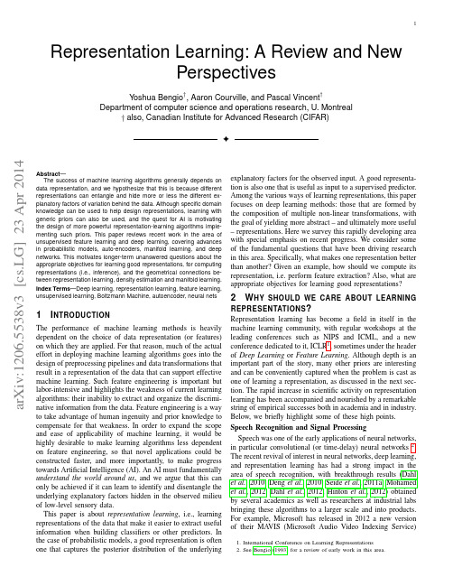
Agar and broth dilution methods to determine the minimal inhibitory concentration (MIC)of antimicrobial substancesIrith Wiegand,Kai Hilpert &Robert E W HancockCentre for Microbial Diseases and Immunity Research,University of British Columbia,2259Lower Mall Research Station,Vancouver,British Columbia,V6T 1Z4,Canada.Correspondence should be addressed to R.E.W.H.(bob@cmdr.ubc.ca).Published online 17January 2008;doi:10.1038/nprot.2007.521The aim of broth and agar dilution methods is to determine the lowest concentration of the assayed antimicrobial agent (minimal inhibitory concentration,MIC)that,under defined test conditions,inhibits the visible growth of the bacterium being investigated.MIC values are used to determine susceptibilities of bacteria to drugs and also to evaluate the activity of new antimicrobial agents.Agar dilution involves the incorporation of different concentrations of the antimicrobial substance into a nutrient agar medium followed by the application of a standardized number of cells to the surface of the agar plate.For broth dilution,often determined in 96-well microtiter plate format,bacteria are inoculated into a liquid growth medium in the presence of different concentrations of an antimicrobial agent.Growth is assessed after incubation for a defined period of time (16–20h)and the MIC value is read.This protocol applies only to aerobic bacteria and can be completed in 3d.INTRODUCTIONAgar dilution and broth dilution are the most commonly used techniques to determine the minimal inhibitory concentration (MIC)of antimicrobial agents,including antibiotics and other substances that kill (bactericidal activity)or inhibit the growth (bacteriostatic activity)of bacteria.The methods described here are targeted for testing susceptibility to antibiotic agents as opposed to other antimicrobial biocides such as preservatives and disinfectants.However,there are no major reasons why they cannot be used for these other antimicrobials.For agar dilution,solutions with defined numbers of bacterial cells are spotted directly onto the nutrient agar plates that have incorporated different antibiotic concentrations.After incubation,the presence of bacterial colonies on the plates indicates growth of the organism.Broth dilution uses liquid growth medium containing geometrically increasing concentrations (typi-cally a twofold dilution series)of the antimicrobial agent,which is inoculated with a defined number of bacterial cells.The final volume of the test defines whether the method is termed macro-dilution,when using a total volume of 2ml,or microdilution,if performed in microtiter plates using r 500m l per well.After incubation,the presence of turbidity or a sediment indicates growth of the organism.In both the agar and the broth dilution approaches,the MIC is defined as the lowest concentration (in mg l À1)of the antimicrobial agent that prevents visible growth of a microorganism under defined conditions.In clinical practice,this in vitro parameter is used to classify the tested microorganism as either clinically susceptible,intermediate or resistant to the tested drug.The interpretative standards for these classifications are published by different national organi-zations such as the Clinical and Laboratory Standards Institute (CLSI)1in the USA and the European Committee on Antimicrobial Susceptibility T esting (EUCAST)2.Breakpoints (the particular MIC that differentiates susceptible,and assumingly treatable,from resistant and assumingly untreatable organisms)are derived from microbiological and clinical experience,and can vary according to the particular species being examined and the particularantimicrobial agent.Features that define these breakpoints are MIC distributions of relevant species,pharmacodynamics and pharmacokinetics of the antimicrobial agent,and clinical outcome data.Resistance (above the breakpoint)is associated with a high likelihood of therapeutic failure,whereas susceptibility is associated with a greater probability of therapeutic success.For isolates classified as intermediate,the therapeutic effect is uncertain 3.MIC determinations can be used for monitoring the develop-ment of antibiotic drug resistance.MIC wild-type distribution databases are available for relevant species–drug combinations ().The highest MIC of the wild-type popu-lation is defined as the ‘epidemiological cut-off value’or wild-type (WT)cut-off value 3(Fig.1).Organisms with acquired resistance can be easily identified by showing higher MIC values than the epidemiological cut-off value.As even slight changes may become clinically relevant,the determination of MIC is a valuable means for resistance surveillance,as well as providing a valuable comparatorp u o r G g n i h s i l b u P e r u t a N 8002©n a t u r e p r o t o c o l s/m o c .e r u t a n .w w w //:p t thN u m b e r o f t e s t e d i s o l a t e sFigure 1|Distribution of MIC values for different isolates for given species (modified from Wiegand and Wiedemann 27).NATURE PROTOCOLS |VOL.3NO.2|2008|163for variants of a given antimicrobial agent and/or species with differential susceptibility.Indeed for new drug candidates,the MIC determination is one of the first steps to evaluate the antimicrobial potential.Specialized protocols can also allow inferences to be drawn regarding resistance mechanisms.For example,results from broth dilution MIC determination with certain b -lactam antibiotics (cefotaxime,cefpodoxime and/or ceftazidime)in the presence or absence of an inhibitor (clavulanic acid)can indicate the produc-tion of extended-spectrum b -lactamases when MICs are at least three twofold concentration steps lower in the presence of the b -lactamase inhibitor 1.Epidemiological resistance data further-more provide the basis for appropriate first-line therapy recom-mendations for empirical treatment.Dilution methods are considered as reference methods for in vitro susceptibility testing and are also used to evaluate the performance of other methods of susceptibility testing.Crucial parametersAs the test results vary widely under different test conditions,the procedures have to be standardized for intra-and inter-laboratory reproducibility.The protocols described here are adjusted to a step-by-step format and follow the guidelines of the two established organizations and committees,the CLSI 1and EUCAST 2.Modifica-tions are introduced for testing the susceptibility to cationic antimicrobial peptides and other cationic agents that tend to bind to surfaces.If implemented rigorously according to the procedures described herein,these modifications allow the generation of reliable data that will be comparable between different laboratories.The use of all methods of this protocol is limited to aerobic bacteria that grow well within 24h in the CLSI and EUCAST recommended test Mueller–Hinton growth medium.Mueller–Hinton broth (MHB)is a general purpose medium that can be used for cultivation of a wide variety of nonfastidious microorgan-isms.For growth of fastidious organisms,such as Streptococcus spp.,Haemophilus influenzae ,Neisseria gonorrheae ,Helicobacter pylori and Campylobacter spp.,the broth needs to be supplemented;furthermore,enrichment of the incubation atmosphere with CO 2and an extension of the incubation time may be necessary for growth.For these species,specific recommendations for medium composition and for test conditions can be found in the CLSI guidelines 1.MediumT o produce accurate and reproducible results,a number of addi-tional requirements must be fulfilled by the test medium for certain antibiotics or antibiotic/species combinations:Correct susceptibility testing of tetracyclines 4,5,daptomycin for gram-positive bacteria 6and aminoglycosides for Pseudomonas aeruginosa 5in broth medium is dependent on the content of Ca 2+and Mg 2+ions.Non-cation-adjusted (unsupplemented)MHB contains in general inadequate amounts of Ca 2+and Mg 2+ions (information given by manufacturer).The broth,therefore,needs to be supplemented with divalent cations when testing the abovementioned antibiotics and/or antibiotic-species combina-tions.The final concentration should be 20–25mg Ca 2+and 10–12.5mg Mg 2+per liter 1,which reflects the divalent cation concentration in blood.Cation-adjusted MHB is commerciallyavailable and only needs to be further supplemented with Ca 2+in case of daptomycin susceptibility testing,as the recommended calcium concentration for testing this antibiotic is 50mg l À1(ref.1).Please note however that cation-adjusted MHB should not be used when testing the activity of cationic antimicrobial peptides,as the presence of Ca 2+and Mg 2+ions causes a substantial inhibition of the cationic peptides’activity 7,8.Mueller–Hinton agar (MHA)needs to be supplemented with 2%(wt/vol)sodium chloride for testing susceptibility of Staphylococcus aureus to methicillin,oxacillin and nafcillin 1.Methicillin-resistant S.aureus (MRSA)are often heteroresistant with resistant and susceptible cells in the same culture and supplementation with NaCl enhances the expression of hetero-geneous resistance 9.T o avoid the adsorption of dalbavancin to plastic surfaces,the addition of polysorbate 80to broth at a final concentration of 0.002%(vol/vol)is recommended.Refer to the CLSI guidelines 1when testing this antibiotic.High levels of thymidine and thymine interfere with suscept-ibility testing of sulfonamides and trimethoprim 10.Contrary to the Difco MHB (not cation-adjusted),the BBL MHB (not cation-adjusted)is not explicitly formulated to have a low thymine and thymidine content.So,according to the manufac-turer,only the former may be used for broth dilution antimi-crobial susceptibility testing.Tigecycline is prone to oxidation,and it seems that its activity is affected by the amount of dissolved oxygen in the medium,which increases with the age of the broth.So,for broth dilution MIC tests with tigecycline,it is necessary to use fresh cation-adjusted MHB (o 12h after autoclaving)11.BacteriaThe bacteria subjected to antimicrobial susceptibility testing must be isolated in pure culture and should have been identified at the genus and species level.Most organisms are available from hospital laboratories,the American Type Culture Collection or other national collections (see Table 1).InoculumThe standardization of the bacterial cell number used for suscept-ibility testing is of critical importance for obtaining accurate and reproducible results.The recommended final inoculum size for broth dilution is 5Â105colony-forming units (cfu)ml À1;thep u o r G g n i h s i l b u P e r u t a N 8002©n a t u r e p r o t o c o l s/m o c .e r u t a n .w w w //:p t t h TABLE 1|Control organisms for antimicrobial susceptibility testing.Identical to ATCC strain Escherichia coli ATCC 25922NCTC 12241,CIP 76.24,DSM 1103Pseudomonas aeruginosa ATCC 27853NCTC 12934,CIP 76.110,DSM 1117Staphylococcus aureus ATCC 29213NCTC 12973,CIP 103429,DSM 2569Enterococcus faecalis ATCC 29212NCTC 12697,CIP 103214,DSM 2570ATCC,American Type Culture Collection,P.O.Box 1549,Manassas,VA 20108,USA;NTCT,NationalCollection of Type Cultures,Health Protection Agency,61Colindale Avenue,London NW95EQ,UK;CIP,Collection de l’Institut Pasteur,25–28Rue de Docteur Roux,75724Paris Cedex 15,France;DSMZ,Deutsche Sammlung von Mikroorganismen und Zellkulturen,Inhoffenstra e 7B,38124Braunschweig,Germany.164|VOL.3NO.2|2008|NATURE PROTOCOLSappropriate cell number in agar dilution experiments is set at 104cfu per spot.Higher inocula can lead to an increase in the MIC particularly if the tested bacterium produces an enzyme capable of destroying the antibiotic.An inoculum effect (e.g.,an eightfold or greater MIC increase upon testing with a 100-fold higher inoculum than recommended)is frequently seen when testing b -lactam suscept-ibility for isolates that produce b -lactamases that are able to inactivate b -lactam antibiotics 12.Lighter inocula than recom-mended may give artificially lower e of inocula with o 5Â105cfu ml À1in broth microdilution can lead to false-susceptible results as described for the detection of methicillin resistance in S.aureus 13and for resistance to certain b -lactams in b -lactamase overproducing Klebsiella oxytoca isolates 14.A fresh pure culture should be used for the preparation of the inoculum.T o avoid the selection of an atypical variant clone,bacteria from four to five normal-appearing colonies are taken to prepare a bacterial suspension with a density equivalent to 108cfu ml À1,which is later used for inoculation.Several options are available for the generation of the bacterial suspension (direct colony suspension into liquid and growth methods using either fresh or overnight cultures).The density of the cell suspension can be assessed spectrophotometri-cally for testing a small number of different bacterial isolates (n o 5).For a larger number of different bacterial isolates,to save time,a turbidity standard can be used as a visual parison between the standards and the turbidity of the bacterial suspensions will in fact point the researcher toward the appropriate dilution for the suspension.The turbidity of a so-called McFarland 0.5standard is equal to 1–2Â108cfu ml À1.McFarland 0.5turbidity standards are commercially available from several manufacturers (e.g.,bioMerieux,cat.no.70900or Scientific Device Laboratory).Alternatively,a BaSO 4turbidity standard equaling the McFarland 0.5standard can be prepared as described below.Once the bacterial suspension is adjusted,it must be used within 30min to avoid changes in the cell number 2.All protocols described here contain a paragraph on how to determine whether the correct inoculum density was used for the susceptibility testing.If the MIC tests are carried out in a laboratory on a routine basis,the cell counts of the inoculum need to be determined only periodically.For all other users,we recommend validating the accuracy of procedures for every test.Quality controlT o verify that the susceptibility results are accurate,it is necessary to include at least one control organism with every batch of MIC determinations.Control organisms are available from different strain collections (Table 1).The MICs for routinely used antibiotics for the quality control organisms are published 1,2and the test values for the control strains should be within the published range to be considered acceptable.LimitationsThe MIC value does not give an indication of the mode of action (cidal or static)of the antimicrobial agent.Within the MIC well or tube or on the agar plate with no visible growth,there may still be viable cells if the drug had a bacteriostatic effect on the bacterial species tested.Growth may resume after the removal of the drug.Alternatively,there may be partial inhibition resulting in impaired and reduced growth rates and consequently no visible growth within the time given.Both phenomena are different from the action of a bactericidal drug,which causes irreversible damage leading to cell death.Furthermore,even with the knowledge of the mode of action of an antimicrobial agent,the MIC value alone is a poor predictor of the efficacy of the drug in vivo .Factors that affect the response to therapy are far more complex and include host defense mechan-isms,underlying diseases of the patient,the site of infection,and the pharmacokinetic and pharmacodynamic properties of the drugs 15.Alternative method for determining MIC valuesMICs for commonly used antibiotics can be obtained using an agar diffusion method with commercially available strips containing an exponential gradient of antibiotic (Etest;AB Biodisk).The antibiotic diffuses into the agar medium inoculated with a lawn culture of the test organism.After overnight incubation,the MIC is read at the point of intersection of an elliptical growth inhibition zone with the strip that has an MIC scale printed on it.This test has been evaluated for a variety of bacteria/antibiotic combinations 16–21and is rapid and easy to use;however,it is limited to the antibiotic range supplied by the manufacturer and is an expensive test to use for screening.Several automated systems for antimicrobial susceptibility test-ing and identification of clinically relevant bacteria are now commercially available,e.g.,Phoenix Automated MicrobiologySystem (BD Diagnostic Systems),the VITEK 2System (bioMe ´r-ieux)and the MicroScan WalkAway-96System (Dade Behring).These systems are cost effective for clinical laboratories with a high throughput of clinical specimens.Fully automated systems reduce the time for setup and,depending on the system,also reduce the time to produce results compared to conventional tests.Moreover,they offer convenient interfaces with laboratory and hospital information systems.However,when testing certain organism-antimicrobial combinations limitations on the accuracy of the assessment of MIC values by these systems are known 22,23.Experimental designAs there are alternative routes for generating the bacterial suspen-sion with different time requirements and alternative methods to determine MIC values with potential pause point options that require advance planning of the workflow,the experiment should be carefully designed by the user before starting the protocol.The flowchart in Figure 2illustrates how the different stages are coordinated.Please examine this figure carefully to make an informed choice as to which experimental approach to embark on.MATERIALSREAGENTS.MHB (Difco;BD Diagnostics,cat.no.275730)sterilized by autoclaving .Mueller–Hinton II broth (cation-adjusted (CAMHB);BBL,BD Diagnostics,cat.no.212322)sterilized by autoclaving.MHA (Difco;BD Diagnostics).Agar,T echnical (Difco;BD Diagnostics,cat.no.281230).Solution A:0.02%acetic acid (Fisher)containing 0.4%BSA (BoehringerMannheim)p u o r G g n i h s i l b u P e r u t a N 8002©n a t u r e p r o t o c o l s/m o c .e r u t a n .w w w //:p t t h NATURE PROTOCOLS |VOL.3NO.2|2008|165.Solution B:0.01%acetic acid containing 0.2%BSA.Preparation of McFarland Standard 0.5:BaCl 2Á2H 2O (Sigma-Aldrich,cat.no.B0750),H 2SO 4(Fluka,cat.no.84721)!CAUTION H 2SO 4is very corrosive/toxic;handling must be performed under the hood;wear acid-resistant gloves and protective clothing (see REAGENT SETUP)..Cation adjustment:MgCl 2Á6H 2O (Fluka,cat.no.63072),CaCl 2Á2H 2O (Fluka,cat.no.21101).Physiological saline [0.9%(wt/vol)NaCl]sterilized by autoclaving EQUIPMENT.Spectrophotometer suitable for measuring at wave lengths of 600and 625nm.For antibiotics:sterile 96-well microtiter plates.We recommend polystyrene plates (BD Falcon;Fisher Scientific,cat.no.351177)for most antimicrobials as these are easier to read at the end of the experiment.For cationic antimicrobial agents such as peptides:96-well polypropylene microtiter plates (Costar,cat.no.3790)!CAUTION Avoid tissue culture treated or polystyrene plates as these are strongly negatively charged and will nonspecifically bind peptides..Eppendorf polypropylene microcentrifuge tubes,1.5ml (Fisher Scientific,cat.no.05-402-24B),sterilized.Screw-capped glass tubes,13Â100mm (Fisher Scientific,cat.no.14-930-10A).48-Pin replicator (Boekel Scientific,cat.no.140501)for inoculating agar dilution plates.Shaker,suitable for test tubes 13Â100mm.Parafilm (Pechiney Plastic Packaging;Fisher Scientific,cat.no.13-374-10).Glass tubes,13Â100mm (VWR International,cat.no.47729-572)with cap (Utech Products,cat.no.1017622),sterilized .Erlenmeyer flasks.Sterile petri dishes,15Â100mm (Fisherbrand;Fisher Scientific,cat.no.08-75-712).0.2-m m pore size cellulose acetate filters (Nalgene;Fisher Scientific,cat.no.190-2520).Cell spreader (Fisherbrand;Fisher Scientific,cat.no.08-100-11).Inoculation loop or cotton swabs (sterilized by autoclaving).Vortex mixerREAGENT SETUPPreparation of McFarland 0.5BaSO 4turbidity standard Prepare a 1.175%(wt/vol)barium chloride dihydrate (BaCl 2Á2H 2O)solution (0.048mol l À1BaCl 2)and a 1%(vol/vol)sulfuric acid (H 2SO 4)solution (0.18mol l À1,0.36N).Add 0.5ml of the 1.175%BaCl 2solution to 99.5ml of the 1%H 2SO 4solution with constant stirring to get a suspension.Measure the optical density of the turbidity standard using a spectrophotometer with a 1cm light path length.The correct absorbance at 625nm should be 0.08–0.13.Aliquot 4–6ml into screw-capped glass tubes.The tubes should have the same size as those for preparing the bacterial suspension for inoculation.Seal tubes tightly withParafilm and store in the dark at room temperature (20–23.51C).Standards are p u o r G g n i h s i l b u P e r u t a N 8002©n a t u r e p r o t o c o l s/m o c .e r u t a n .w w w //:p t t h Pure cultures of bacterial isolates (test and control)Day 1Day 2orPrior to testing (2 d required)Prepare overnight culturesPrepare media (store at 4 °C) and antibioticstock solutions (freeze)Antimicrobial susceptibility testing— part I Determine the cell count inovernight culturesPreparation of bacterial suspensionIncubate on nonselectiveagar overnightoror orSuspension with 1–2 × 108cfu/mlTake sample for cell count (ifused for agar dilution)Colony suspensionAdjust turbidity using a McFarland Standard 0.54–6 h growth methodPrepare overnight cultures inliquidGrowth method using overnight culturesAdjust turbidity using a spectrophotometerPrepare agar plates with antibiotics[Day 1 may be possibledepending on the antibiotic (store at 4 °C)]orororPreparebroth macro dilutions of antibioticPrepare broth micro dilutions of antibioticPrepare broth micro dilutions of peptideAntimicrobial susceptibility testing— part ll[Day 1 may be possible (freeze)]Inoculate agarplatesorInoculate broth macro dilutions of antibioticororTake sample for cell countRead MICsInoculate broth micro dilutions of peptideInoculate broth micro dilutions of antibioticDetermine cell countDay 3Figure 2|Flowchart for antimicrobial susceptibility testing.166|VOL.3NO.2|2008|NATURE PROTOCOLSstable for at least a month.!CAUTION H 2SO 4is corrosive/toxic;wear appro-priate safety clothing when handling concentrated H 2SO 4.Preparation of antibiotic-free nutrient-rich agar plates Prepare agar med-ium according to the manufacturer’s instructions.Alternatively,use nutrient-rich broth according to the manufacturer’s instructions and add 1.7%agar (17g agar per liter)before autoclaving.Approximately 20–25ml is necessary to pour one 15Â100mm petri dish.After autoclaving (e.g.,1211C,15min,1bar),cool the medium to 50–601C.Pour agar into the petri dishes and allow to set.Dry the surface of the agar plates either in an incubator or in a laminar air flow hood for 30min with the lid ajar.Store agar plates in plastic bags in inverted position (bottom facing up)at 41C.Adjustment of cation content of MHB medium (20–25mg Ca 2+and 10–12.5mg Mg 2+per liter)Prepare a 10mg ml À1Mg 2+stock solution by dissolving 8.36g of MgCl 2Á6H 2O in 100ml deionized water.Prepare a 10mg ml À1Ca 2+stock solution by dissolving 3.68g of CaCl 2Á2H 2O in 100ml deionized water.Filter-sterilize both stock solutions using 0.2-m m pore size cellulose-acetate filters.Prepare MHB according to the manufacturer’s instructions,autoclave and cool the medium to 2–81C before the addition of the cation solutions.Add 100m l of stock solution per 1mg l À1needed for 1l of medium.For example,add 2ml of Ca 2+stock solution if 20mg needs to be added to 1l MHB.Stock solution of the antimicrobial agent Antimicrobial agents should be stored in the dark at 41C in sealed containers containing a desiccant unless recommended otherwise by the manufacturer.We advise the storage ofantimicrobial peptides at 201C.Before weighing the antimicrobial agent,let the container warm at room temperature for B 2h to avoid condensation of water on the powder.Antibiotics are generally supplied by the manufacturer with the information about the potency (m g per mg powder)that needs to be taken into consideration when weighing the agent.For antibiotics,prepare a stock solution at 10mg ml À1when planning to use it for agar dilution (Step 4A).For broth dilution tests (Steps 4B and 4C)set up a stock solution with a concentration atleast ten times higher than the highest concentration to be tested.For testing antimicrobial peptides (Steps 4D and 4E),prepare a 20-fold concentrated stock e the following formula for calculating the right amount of antibiotic to be weighed (this does not apply to antimicrobial peptides):W ¼ðC ÂV ÞPwhere,W ¼weight of antimicrobial agent in milligram to be dissolved;V ¼desired volume (ml);C ¼final concentration of stock solution (m g ml À1);P ¼potency given by the manufacturer (m g mg À1).Use sterile containers and spatula for weighing the antimicrobial agent and dissolve in sterile distilled water or in the recommended solvent.A list ofsolvents for frequently used antibiotics is found in ref.24.Antibiotic solutions can be filter-sterilized using a 0.2-m m pore size cellulose-acetate filter.However,it has to be ascertained that the antibiotic does not bind to cellulose acetate (information that is sometimes given by the manufacturer).Do not filter-sterilize antimicrobial peptides,which tend to bind to anionic surfaces like cellulose acetate.Always use the fresh antibiotic stock solution for broth microdilution if it is planned to freeze the antibiotic containing microtiter plates at 701C for later usage.For other applications,aliquot the stocksolution.The volume of the aliquots depends on the downstream applications and in general one aliquot should contain the volume needed for one test.Containers need to be sterile,cold resistant and should seal tightly (e.g.,for smaller volumes sterile Eppendorf tubes can be used).Store the aliquots at 201C or below unless it is instructed otherwise by the manufacturer.Most antimicrobial agents are stable at À601C for at least 6months.Stability and storage information for frequently used antibiotics can be found in ref.24.Do not refreeze thawed stock solutions.Some antimicrobials,particularly b -lactams antibiotics,can degrade when thawed and refrozen repeatedly 1.PROCEDUREPreparation of the bacterial suspensionTIMING B 5min per isolate/overnight pause point1|Streak the bacterial isolates to be tested (including a control organism)onto nutrient-rich (e.g.,Mueller–Hinton)agar plates without inhibitor to obtain single colonies.2|Incubate plates for 18–24h at 371C.3|Different methods for the preparation of the inoculum can be used.Direct suspension of overnight colonies into broth or sterile saline solution (option A)is a very convenient method that can be used for most bacterial species.It is particularlyrecommended for fastidious organisms such as Streptococcus spp.,Haemophilus spp.and Neisseria spp.For some strains within a species,unpredictable clumping can occur with option A.Consequently,when colonies are difficult to suspend and an even suspension is difficult to achieve,freshly grown broth cultures can be diluted (option B).As an alternative to a freshly grown culture,an overnight broth culture can also be used (option C)according to the user’s preference.This method is not part of CLSI or EUCAST recommendations;however,the option to use overnight cultures is given in the guide to antimicrobial susceptibility testing of the British Society of Antimicrobial Chemotherapy 24.(A)Colony suspension methodTIMING B 5min per isolate (i)Prepare the antibiotic or peptide dilutions.(ii)For each isolate,select three to five morphologically similar colonies from the fresh agar plate from Step 2and touchthe top of each selected colony using a sterile loop or cotton swab.Transfer the growth into a sterile capped glass tube containing sterile broth or saline solution.Mix using a vortex mixer.(iii)Turbidity can be assessed visually by comparing the test and the McFarland Standard.Mix the McFarland 0.5BaSO 4stan-dard vigorously using a vortex mixer.Please note that commercially available standards containing latex particles should not be vortexed,but gently inverted several parison against a white background with contrasting black lines and good lighting are helpful.Alternatively,the turbidity can be verified measuring the absorbance of the suspension spectrophotometrically.The absorbance should be in the same range as that of the McFarland standard 0.5(OD625nm should be at 0.08–0.13).(iv)Adjust the suspension’s turbidity to that of a McFarland Standard 0.5by adding sterile distilled water,saline or broth,ifthe turbidity is too high,or by adding more bacterial material if is too low.m CRITICAL STEP After turbidity adjustment,the bacterial suspension should be used within 30min,as the cell number might otherwise change.p u o r G g n i h s i l b u P e r u t a N 8002©n a t u r e p r o t o c o l s/m o c .e r u t a n .w w w //:p t t h NATURE PROTOCOLS |VOL.3NO.2|2008|167。

汉英心理学常用词汇［人格］表面特质 surface traitⅠ型错误 type Ⅰ error Ⅱ型错误 type Ⅱ errorF 分布 F distributionF 检验 F testt 分布 t distributiont 检验 t testz 分数 z scorez 检验 z testφ系数 φ coefficientχ2分布 chi-square distributionχ2检验 chi-square testχ2可加性 additivity of chi-square艾森克人格问卷 Eysenck Personality Questionnaire, EPQ爱德华兹个人爱好量表 Edwards Personal Preference Schedule, EPPS 白板说 theory of tabula rasa百分等级 percentile rank贝利婴儿发展量表 Bayley Scales of Infant Development贝叶斯定理 Bayes’ theorem备择假设 alternative hypothesis比率量表 ratio scale比率智商 ratio intelligence quotient比内-西蒙智力量表 Binet-Simon Scale of Intelligence变异系数 coefficient of variation标准差 standard deviation标准分数 standard score标准化测验 standardized test标准九分 stanine标准误差 standard error标准正态分布 standard normal distribution表面效度 face validity参数 parameter参数估计 parameter estimation参数统计检验 parametric statistical test操作测验 performance test测量误差 measurement error测验标准化 test standardization测验法 test method测验分数 test score测验焦虑test anxiety测验偏向test bias测验手册test manual测验特征函数test characteristic function测验项目test item差异量数measure of difference差异显著性significance of difference常模norm常模参照测验norm-referenced test场独立性field independence场依存性field dependence称名量表nominal scale成就测验achievement test抽样sampling抽样分布sampling distribution处理均方mean square of treatment创造性人格creative personality次要特质secondary trait丹佛儿童发展筛选测验Denver Development Screening Test 单尾检验one-tailed test单因素方差分析one-factor analysis of variance导出分数derived score等距量表interval scale等值复本equivalent forms邓肯多重范围检验Duncan multiple-range test地位人格status personality点二列相关point biserial correlation调和平均数harmonic mean独立性检验test of independence多项选择法multiple choice method多元分析multiple analys is多元回归multiple regression多重比较multiple comparison多重相关multiple correlation儿童统觉测验Children’s Apperception Test二列相关biserial correlation二项分布binomial distribution二元论dualism泛心［灵］论panpsychism方差variance方差分析analysis of variance, ANOVA方差齐性homogeneity of variance非参数检验non-parametric test费希尔Z转换Fisher’s Z transform ation分半信度split-half reliability分层抽样stratified sampling符号检验sign test负相关negative correlation副现象论epiphenomenalism概化理论generalizability theory, GT感觉主义sensationalism格塞尔发展测验Gesell Development Test个别测验individual test构想效度construct validity古迪纳夫-哈里斯画人测验Goodenough-Harries Drawing Test合成分数composite score机能系统理论theory of functional system积差相关product-moment correlation极大似然法maximum likelihood method集中量数measure of central tendency集中趋势central tendency几何平均数geometric average计算机化适应性测验computerized adaptive test加权平均数weighted mean家庭调查表home inventory假设检验hypothesis testing间接测量indirect measurement检验能力power of test检验统计量statistic of test鉴别指数discrimination index交叉效度分析cross validation交互作用interaction焦虑anxiety教师自编测验teacher-made test进攻性aggresiveness经典测验理论classical test theory, CTT经验心理学empirical psychology警察心理测验mental test for police拒绝域rejection region聚类分析cluster analysis均方mean square考夫曼儿童评估测验Kaufman Assessment Battery for Children, K-ABC 克龙巴赫α系数Cronbach’s α coefficien t客观测验objective test客观题objective item肯德尔和谐系数Kendall’s concordance coefficient肯德尔一致性系数Kendall’s consistency coefficient控制源locus of control库德-理查森信度Kuder-Richardson reliability跨文化测验cross-cultural test雷文推理测验Raven’s Progressive Matrices Test类型论type theory离差deviation离差平方和sum of deviation square离差智商deviation intelligence quotient离中趋势divergence tendency理论心理学theoretical psychology理性心理学rational psychology理性主义rationalism利克特量表Likert Scale连续变量continuous variable联想主义associationism两阶段抽样法two-stage sampling量表值scale value列联表contingency table临床测验clinical test临界值critical value零相关zero correlation陆军甲种测验Army Alpha Test罗杰斯自我论Rogers’ self theory马尔计算理论Marr’s computational theory马克思主义心理学Marxist psychology曼-惠特尼U检验Mann-Whitney U test描述统计descriptive statistics明尼苏达多相人格调查表Minnesota Multiphas ic Personality Inventory, MMPI 墨迹测验inkblot test目标参照测验criterion referenced test内容效度content validity纳格尔图片测验Nagel Chart Test难度测验power test能力测验ability test能力倾向测验aptitude test纽曼-科伊尔斯检验Newman-Keuls test判别分析discriminant analysis皮尔逊相关系数Pearson’s correlation coefficient偏回归partial regression偏态分布skewed distribution平行测验parallel test平行复本parallel forms评定法rating method评定量表rating scale评定者误差rater’s error评分者信度scorer reliability迫选测验forced-choice test潜在特质理论latent trait theory, LTT情境测验situational test区分能力倾向测验Differential Aptitude Test, DAT区分效度discrimination validity趋势检验trend test全距range人格personality人格测验personality test人格结构personality structure人格理论theory of personality人格面具persona人格心理学personality psychology认识论epistemology散点图scatterplot色盲测验color blindness test神经心理测验neuropsychological test生活事件量表life event scale剩余标准差residual standard deviation十六种人格因素问卷Sixteen Personality Factor Questionnaire, 16PF 时限time limit实验控制experimental control实证效度empirical validity适合度检验goodness of fit test双峰分布bimodal distribution双盲double blind双尾检验two-tailed test顺序量表ordinal scale思维型thinking type斯皮尔曼-布朗公式Spearman-Brown formula斯皮尔曼等级相关Spearman’s rank correl ation斯泰尔-克劳福德效应Stile-Crawford effect斯坦福-比内智力量表Stanford-Binet Intelligence Scale斯特朗-坎贝尔兴趣调查表Strong-Campbell Interest Inventory四分[位]差quartile deviation, Q速度测验speed test算术平均数arithmetic mean, AM随机抽样random sampling随机化randomization随机区组设计randomized block design态度量表attitude scale特质trait特质论trait theory填充测验completion test同时效度concurrent validity同质性homogeneity统计分析statistical analysis统计概率statistical probability统计决策statistical decision统计显著性statistical significance投射测验projective test团体测验group test推论统计inferential statistics完全随机化设计completely randomized design威尔科克森符号秩次检验Wilcoxon’s sign rank test韦克斯勒成人智力量表Wechsler Adult Intelligence Scale, WAIS韦克斯勒儿童智力量表Wechsler Intelligence Scale for Children, WISC 文化公平测验culture fair test无偏估计量unbiased estimator误差均方error mean square析因设计方差分析analysis of variance of factorial design系统误差systematic error显著性水平significance level线性关系linear relationship线性回归linear regression相关correlation相关矩阵correlation matrix相关系数coefficient of correlation相容效度congruent validity项目反应理论item response theory, IRT项目分析item analysis项目难度item difficulty项目区分度item discrimination项目特征函数item characteristic function项目特征曲线item characteristic curve项目选择item selection小概率事件small probability event效标criterion效标关联效度criterion-related validity效度validity校正数correction协方差分析analysis of covariance心理测量学psychometrics心理测验mental test, psychological test心理分析mental analys is心理量表mental scale心理年龄mental age心理统计学psychological statistics心理物理量表psychophysical scale心理现象系统system of mental phenomena心理学方法论methodology in psychology心理学史history of psychology心理学体系system of psychology心理学系统观systematic approach in psychology心理主义mentalism心身平行论mind-body parallelism心身问题mind-body problem心身相互作用论mind-body interactionism新生儿行为评价量表Neonatal Behavioral Assessment Scale 信度reliability信息函数information function兴趣测验interest test虚无假设null hypothesis选拔与安置测验selection and placement test学业成就测验academic achievement test延迟满足delay of gratification样本sample一般能力测验general ability test一元论monism因变量dependent variable因素分析factor analys is因素负荷factor loading因素效度factorial validity英国经验主义British empiricism又称“变异数”。

英语二大纲词汇汇总一、New words and expressionsNew words1. critical adj. 有推断力的；推断公正〔或审慎〕的2. non-fiction n. 纪实文学3. position n. 观点；态度；立场4. statement n. 说明；说法；表态5. question v. 表示疑问；疑心out of question / out of the question6. evaluate v. 估量；评价；评估7. context n. 事情发生的背景，环境，来龙去脉8. value n. values pl.]是非标准；价值观valuableinvaluable=pricelessvalueless9. represent v. 描述；表现representative adj./n.10. assertion n. 明确肯定；断言11. sufficient adj. 足够的；充分的sufficiencyinsufficient12. statistic n. statistics pl.]统计数字；统计资料13. integrate v.〔使〕合并，成为一体14. authority n.专家；学术权威；泰斗an/the authority on sth.authorize15. compare v. 比拟；比照compare A with Bcompare A to B16. subject n. 主题；题目；题材17. consistent adj. 相符的；符合的18. inconsistency n. 不一致19. assumption n. 假定；假设20. case n. 具体情况；事例in casein case of firein case that…a case in pointconfirmed/suspected cases21. directly adv. 直接地；径直地22. identify v. 找到；发觉23. valid adj. 符合逻辑的；合理的；确凿的validity n. 有效性，正确〔性〕invalid24. credible adj. 可信的；可靠的incredible=unbelievable25. landmark n.〔标志重要阶段的〕里程碑26. relevant adj. 紧密相关的；切题的relevancy n. 关联；恰当irrelevant27. current adj. 现时发生的；当前的28. appropriate adj. 适宜的；恰当的inappropriateIt's (not) appropriate that ….29. bias n. 偏见；偏心；偏向30. considerably adv. 非常；很；相当多地considerconsideringconsiderableconsiderateconsideration31. Democrat n. 〔美国〕民主党党员，民主党支持者民32. Republican n. 〔美国〕共和党党员，共和党支持者33. reflect v. 显示；说明；表达34. informed adj. 有学问的；有见识的well-informedill-informedPhrases and Expressions1. apply to 使用；应用2. put forth 提出；产生3. take …into account 考虑到；顾及4. accept/take …at face value 信任外表；信以为真5. with a grain of salt 有保存地；持疑心态度地二、New words and expressionsNew words1. spill v.〔使〕洒出，泼出，溢出2. respond v. 作出反响；响应respond to…response3. interview v. 〔媒体〕采访，访问4. creative adj. 创作的5. occur v. 发生；出现It occurred to me that…6. remove v. 拿开；去掉7. refrigerator n. 冰箱8. grip n. 紧握；紧抓9. slippery adj. 滑的；滑得抓不住〔或站不稳、难以行走〕10. content n. 所容纳之物；所含之物11. veritable adj. 十足的；名副其实的；不折不扣的12. yell v. 叫喊；大喊；吼叫13. lecture n.〔冗长的〕教训，训斥，责备14. mess n. 肮脏；杂乱；不整洁15. rarely adv. 罕有；很少；不常rare animals / stampsRarely is he late for class.16. puddle n. 水洼；小水坑17. eventually 最后；总算18. restore v. 使复原；使复位；使复职19. sponge n. 海绵块20. effectively adv. 有效地effectiveineffective注意区分：effective / efficient21. tiny adj. 极小的；微小的22. discover v. 了解到；认识到；查明discovery23. grasp v. 抓紧；抓牢24. lip n.〔容器或凹陷地方的)边，边沿25. renowned adj. 有名的；闻名的；受尊敬的26. remark v. 谈论；评论27. opportunity n. 时机；时机28. scientific adj. 科学〔上〕的；关于科学的sciencescientist例如：The medical science is making great progress in the treatment of cancer.You should provide scientific evidence instead of subjective evidence to prove this theory holds water.Several world-renowned scientists will be invited to attend the forum.29. valuable adj. 很有用的；很重要的；珍贵的Phrases and Expressions1. in this manner 用这种方法2. set…apart from 区别；使与众不同三、New words and expressionsNew words1. reflection n. 〔关于某主题的〕思考，回忆2. loyalty n. 忠诚；忠实；忠心耿耿3. recognize v. 成认；意识到4. betray v. 辜负；对…不忠5. indeed adv. 其实；实际上6. virtue n. 高尚的道德；正直的品性；德行7. trend n. 趋势；趋向；倾向；动态；动向8. befriend v. 做〔尤指需要援助者的〕朋友；友善相待9. request v. 〔礼貌或正式地〕请求，要求10. trendy adj. 时髦的；赶时髦的11. multitude n. 众多；大量12. mutual adj. 共有的；共同的mutual respect / understanding辨析：mutual / manual / manure / mature / menu / mental13. term n. 词语；术语：措辞14. site n. 网站；站点15. acronym n. 首字母缩略词16. perish v. 丧失；湮灭；消灭17. thought n. 想法；看法；主意；记忆18. gossip n. 流言蜚语19. challenge v. 考查…的能力；考验…的技巧20. akin adj. 相似的；类似的21. deposit n. 存款22. account n. 账户accountantcurrent accountdeposit account23. interest n. 利息24. well-being n. 健康；安乐；康乐25. welfare n. 〔个体或群体的〕幸福，平安与健康26. essence n. 本质；实质；精髓27. seek v. 寻觅28. notoriety n. 恶名；坏名声notorious 相当于infamous29. premise n. 前提；假定；30. exploit v. 利用〔…为自己谋利〕31. reconnect v. 再联系；再联络32. virtual adj. 〔通过计算机软件，如在因特网上〕模拟的，虚拟的33. assure v. 使确信；向…保证assure X. of sth.assure X. that…34. caution n. 警告；告诫35. lyric n. 歌词36. undisputed adj. 不容置疑的；毫无疑问的；不可争辩的37. generation n. 〔统称〕一代人，同代人，同辈人generation gapfour generations living under the same roofPhrases and Expressions1. stick by 坚持忠于；不离不弃〔某人〕2. through thick and thin 不畏困难险阻go through thick and thin3. lead to 导致，造成〔后果〕4. a multitude of 众多的；大量的5. perish the thought 甭想了；但愿不会如此6. engage in 〔使〕从事，参加7. in essence 本质上8. assure…of…使放心；向…保证9. pay attention to 注意10. warn…of…警告某人某事四、New words and expressionsNew words1. blessing n. 好事；有益之事2. subsistence n. 牵强维持生活；生计3. sugar cane n. 甘蔗4. corn n. 玉米5. hog n. 猪6. cash n. 现金7. dairy adj. 乳品业的；生产乳品的n. 牛奶场；乳制品区分：dairy / diary8. complain v. 抱怨；埋怨；发牢骚complaintcomplain to X. about sth.complain of a splitting headache9. carpenter n. 木工；木匠10. committed adj. 尽心尽力的：坚信的；坚决的commit an errorcommit a crimecommit Xcommit oneself to (doing) sth.be committed to (doing) sth.commitment11. brick n. 砖；砖块12. hammer n. 锤子；榔头13. escort n. 护送者；迎战队14. remind v. 提示；使想起15. victim n. 受害者；牺牲品fall victim to sth.16. ideology n. 意识形态：观念形态17. terrorism n. 恐惧主义18. depression n. 萧条期；经济衰退；不景气depressdepressed 沮丧的；萧条的19. unrest n. 动乱；动乱；骚动20. illegal adj. 不合法的；非法的；违法的il是in的变体，否认前缀，再如：illogicalir, im都是in的变体，如：irregular, irresponsible, imbalanced, impossible, immobile21. immigrant n.〔外来〕移民；外侨22. trafficking n. 非法交易；非法买卖c结尾的词变形时先加k，如trafficker, panicker, picnicker, trafficking, panicking 23. dealer n. 贩毒者；X贩子deal in sth.car / drug dealerdeal with sth.24. gang n. 一帮，一群，一伙〔闹事、斗殴的年轻人〕25. contribute v. 增加；增进；添加〔到某物〕26. quit v. 停止；戒掉Phrases and Expressions1. bring in 赚得；挣2. eke out a living 尽力维持生计；牵强度日3. sink in 被完全理解；被充分意识到4. look forward to 〔快乐地〕盼望，期待5. over and over again 屡次；反复地；一再6. be prepared for 打算好；有所打算7. believe in 认为某事好〔对、可接受〕五、. New words and expressionsNew words1. transcend v. 超出，超越〔通常的界限〕2. incessantly adv. 不停地；延续不断地3. noisily adv. 喧闹地noisenoisy4. subtly adv. 不易发觉地；不明显地；微妙地5. enormity n. 庞大；深远影响；严峻性enormous6. burden n. 〔义务、责任等的〕重担，负担7. belief n. 信任；信心believebelievableunbelievablediXelief8. unique adj. 唯—的；独—无二的；独特的9. affliction n. 折磨；痛苦10. especially adv. 尤其；特别；格外11. tribe n. 部落12. species n. 种，物种〔分类上小于属〕13. discipline n. X力；遵守纪律14. confront v. 处理，解决〔问题或困境〕15. evoke v. 引起，唤起〔感情、记忆或形象〕16. grief n. 〔尤指因某人去世引起的〕悲伤，悲哀，伤心17. guilt n. 内疚；悔恨guiltybe guilty ofbe / feel guilty about18. anxiety n. 焦虑；忧虑anxious19. anguish n. 剧痛；极度痛苦；苦恼20. despair n. 无望21. uncomfortable adj.〔使〕焦虑的，为难的，畏惧的，不自在的22. physical adj. 身体的；肉体的；躯体的23. equal v. 比得上；敌得过24. conflict n. 冲突；争吵；争论25. engender v. 产生，引起〔某种感觉或情况〕26. pose v. 造成〔威胁、问题等〕；引起；产生27. distinguish v. 区分；区分；分清28. wisdom n. 智慧；才智；精明29. mentally adv. 精神上；智力上；思想上30. spiritually adv. 精神上；心灵上31. desire v. 渴望；期望32. deliberately adv. 成心；蓄意；存心33. instruct v. 教授；指导34. dread v. 非常畏惧；极为担忧Phrases and Expressions1. moan about 抱怨2. a series of 系列；连续3. because of 因为4. as well as 除…之外5. cutting edge 〔处于某事物开展的〕尖端，最前沿，领先阶段6. call forth 引起；使产生六、. New words and expressionsNew words1. stationery n. 文具同音词：stationary2. fare n. 车费；船费；飞机票价3. lump sum n. 一次总付的钱款4. recess n. 课间休息，5. allocate v. 拨〔给〕；划〔给〕；分配〔给〕6. overspend v. 花钱过多；比〔估计的〕花得多；超支注意over- / out-的区别：overeat outeatoverdo outdooversleep outliveoverweight outshine7. opt v. 选择；挑选optionoptional8. constraint n. 限制；限定；约束9. budget v. 慎重花钱；把…编入预算10. overindulge v. 过多地享用〔尤指食物或饮料〕11. short-sighted adj. 目光溜浅的；没有远见的12. mentality n. 心态；思想状况；思想方法13. sibling n. 兄；弟；姐；妹14. indulge v. 沉湎，沉迷，沉溺〔于…〕15. rationing n. 定量配给X；配给制16. principle n. 观念；〔行动、思想的〕理由，信条同音词：principal17. unnecessarily adv. 没必要地18. differentiate v. 区分；区别；区分differdifferentdifference19. inculcate v. 反复灌输；谆谆教导20. resist v. 忍住；抵挡resistantresistance21. temptation n. 引诱；诱惑22. scheme n. 方案；方案；体系；体制23. formation n. 组成；形成24. kindergarten n. 幼儿园25. monthly adj. 按月结算的；有效期为一个月的dailyweeklybiweeklymonthlyquarterlyyearlyPhrases and Expressions1. on a daily basis 每日地2. result in 导致3. pay off 付清；偿清4. within one's means 量入为出5. stand…in good stead 〔需要时〕对某人有用，对某人有利七、New words and expressionsNew words1. inner adj. 内心的；隐藏的2. precisely adv. 精确地；恰好地preciseprecision联想：accurate, accuracy比拟：simply, possibly, subtly, truly / definitely, rarely, fortunately, likely / luckily, heavily3. bombard v. 大肆抨击；连珠炮似地质问；提供过多信息，4. dreaded adj. 令人畏惧的；恐怖的5. small talk n. 寒喧；闲谈；聊天6. hesitation n. 犹豫hesitatehesitanthesitancy / hesitation7. wonder v. 想了解；想弄明白；琢磨n. 奇迹wonder wh-…do / work wonders / miracles8. prompt v. 促使；导致；激起9. complete adj. 〔用以强调〕完全的，彻底的10. upset adj. 伤心的；不快乐的；沮丧的11. roll v. 〔使〕翻滚，滚动12. despite prep. 即使；尽管despite / in spite of that fact that …13. feeble adj. 无效的；无力的14. attempt n./ v. 企图；试图；尝试attempted15. wipe v.〔用布、手等〕擦干净，抹掉16. profusely adv. 大量地；连连地17. address v. 写〔收信人〕姓名地址；致函18. receptionist n. 接待员19. attach v. 把…固定，把…附〔在…上〕attach …to…attached 依恋的；附加的；附属的attachment 依恋；附件20. emotion n. 强烈的感情；感情；情绪emotionalemotionless21. contain v. 操纵，克制，抑制〔感情〕22. apparently adv. 据…所知；看来；显然23. overwhelming adj. 庞大的；压倒性的；无法抗拒的overwhelming problemsan overwhelmed person联想：surprised / surprisingexcited / excitingamazed / amazingdisappointed / disappointingfrightened / frighting注意：excited eyes / expressions / looks24. scream v. 高声喊，大声叫Phrases and Expressions1. be lost in one's thought 陷入沉思2. break down 失败3. come up with 找到〔答案等〕；想出4. drop…off 〔顺路〕把…放下5. take one's own life 自杀6. in desperation 在无望中；走投无路7. care about X. 关怀；关怀8. take a chance 冒险9. make a difference 有作用；产生影响The Great Minds名人名言局部补充make A of BA famous quoteA pessimist makes difficulties of his opportunities; an optimist makes opportunities of his difficulties. ----Harry S. Truman悲观者让时机沦为困难；乐观者把困难铸成时机。

相关分析（Correlate）Correlation and dependenceIn statistics, correlation and dependence are any of a broad class of statistical relationships between two or more random variables or observed data values.Correlation is computed（用...计算）into what is known as the correlation coefficient（相关系数）, which ranges between -1 and +1. Perfect positive correlation (a correlation co-efficient of +1) implies（意味着）that as one security（证券）moves, either up or down, the other security will move in lockstep（步伐一致的）, in the same direction. Alternatively（同样的）, perfect negative correlation means that if one security moves in either direction the security that is perfectly negatively correlated will move by an equal amount in the opposite（相反的）direction. If the correlation is 0, the movements of the securities are said to have no correlation; they are completely random（随意、胡乱）.There are several correlation coefficients, often denoted（表示、指示）ρ or r, measuring（衡量、测量）the degree of correlation. The most common of these is the Pearson correlation coefficient, which is sensitive only to a linear（只进行两变量线性分析）relationship between two variables (which may exist even if one is a nonlinear function of the other).Other correlation coefficients have been developed to be more robust（有效的、稳健）than the Pearson correlation, or more sensitive to nonlinear relationships.Rank（等级）correlation coefficients, such as Spearman's rank correlation coefficient and Kendall's rank correlation coefficient (τ) measure the extent（范围）to which, as one variable increases, the other variable tends to increase, without requiring（需要、命令）that increase to be represented by a linear relationship. If, as the one variable（变量）increases（增加）, the other decreases, the rank correlation coefficients will be negative. It is common to regard these rank correlation coefficients as alternatives to Pearson's coefficient, used either to reduce the amount of calculation or to make the coefficient less sensitive to non-normality in distributions（分布）. However, this view has little mathematical basis, as rank correlation coefficients measure a different type of relationship than the Pearson product-moment correlation coefficient, and are best seen as measures of a different type of association, rather than as alternative measure of the population correlation coefficient.Common misconceptions（错误的想法）Correlation and causality（因果关系）The conventional（大会）dictum（声明）that "correlation does not imply causation" means that correlation cannot be used to infer a causal relationship between the variables.Correlation and linearityFour sets of data with the same correlation of 0.816The Pearson correlation coefficient indicates the strength of a linear relationship between two variables, but its value generally does not completely characterize their relationship. In particular, if the conditional mean of Y given X, denoted E(Y|X), is not linear in X, the correlation coefficient will not fully determine the form ofE(Y|X).The image on the right shows scatterplots（散点图）of Anscombe's quartet, a set of four different pairs of variables created by Francis Anscombe. The four y variables have the same mean (7.5), standard deviation (4.12), correlation (0.816) and regression line (y = 3 + 0.5x). However, as can be seen on the plots, the distribution of the variables is very different. The first one (top left) seems to be distributed normally, and corresponds to what one would expect when considering two variables correlated and following the assumption of normality. The second one (top right) is not distributed normally; while an obvious relationship between the two variables can be observed, it is not linear. In this case the Pearson correlation coefficient does not indicate that there is an exact functional relationship: only the extent to which that relationship can be approximated（大概）by a linear relationship. In the third case (bottom left), the linear relationship is perfect, except for one outlier which exerts enough influence to lower the correlation coefficient from 1 to0.816. Finally, the fourth example (bottom right) shows another example when one outlier（异常值）is enough to produce a high correlation coefficient, even though the relationship between the two variables is not linear.(离群值可降低、也可以增加数据的相关性。

Package‘dHSIC’October13,2022Type PackageTitle Independence Testing via Hilbert Schmidt Independence CriterionVersion2.1Date2019-01-04Author Niklas Pfister and Jonas PetersMaintainer Niklas Pfister<*****************.ethz.ch>Description Contains an implementation of thed-variable Hilbert Schmidt independence criterionand several hypothesis tests based on it,as describedin Pfister et al.(2017)<doi:10.1111/rssb.12235>.License GPL-3Imports Rcpp(>=0.12.18)LinkingTo RcppNeedsCompilation yesRepository CRANDate/Publication2019-01-0413:50:19UTCR topics documented:dHSIC-package (2)dhsic (3)dhsic.test (5)Index812dHSIC-package dHSIC-package Independence Testing via Hilbert Schmidt Independence CriterionDescriptionContains an implementation of the d-variable Hilbert Schmidt independence criterion and severalhypothesis tests based on it,as described in Pfister et al.(2017)<doi:10.1111/rssb.12235>.DetailsThe DESCRIPTIONfile:Package:dHSICType:PackageTitle:Independence Testing via Hilbert Schmidt Independence CriterionVersion: 2.1Date:2019-01-04Author:Niklas Pfister and Jonas PetersMaintainer:Niklas Pfister<pfi**************.ethz.ch>Description:Contains an implementation of the d-variable Hilbert Schmidt independence criterion and several hypothesis te License:GPL-3Imports:Rcpp(>=0.12.18)LinkingTo:RcppIndex of help topics:dHSIC-package Independence Testing via Hilbert SchmidtIndependence Criteriondhsic d-variable Hilbert Schmidt independencecriterion-dHSICdhsic.test Independence test based on dHSICAuthor(s)Niklas Pfister and Jonas PetersMaintainer:Niklas Pfister<pfi**************.ethz.ch>ReferencesGretton,A.,K.Fukumizu,C.H.Teo,L.Song,B.Sch\"olkopf and A.J.Smola(2007).A kernelstatistical test of independence.In Advances in Neural Information Processing Systems(pp.585-592).Pfister,N.,P.B\"uhlmann,B.Sch\"olkopf and J.Peters(2017).Kernel-based Tests for Joint Inde-pendence.To appear in the Journal of the Royal Statistical Society,Series B.dhsic d-variable Hilbert Schmidt independence criterion-dHSICDescriptionThe d-variable Hilbert Schmidt independence criterion(dHSIC)is a non-parametric measure of dependence between an arbitrary number of variables.In the large sample limit the value of dHSIC is0if the variables are jointly independent and positive if there is a dependence.It is therefore able to detect any type of dependence given a sufficient amount of data.Usagedhsic(X,Y,K,kernel="gaussian",bandwidth=1,matrix.input=FALSE)ArgumentsX either a list of at least two numeric matrices or a single numeric matrix.The rows of a matrix correspond to the observations of a variable.It is always requiredthat there are an equal number of observations for all variables(i.e.all matriceshave to have the same number of rows).If X is a single numeric matrix than onehas to specify the second variable as Y or set matrix.input to"TRUE".Seebelow for more details.Y a numeric matrix if X is also a numeric matrix and omitted if X is a list.K a list of the gram matrices corresponding to each variable.If K specified the other inputs will have no effect on the computations.kernel a vector of character strings specifying the kernels for each variable.There exist two pre-defined kernels:"gaussian"(Gaussian kernel with median heuristic asbandwidth)and"discrete"(discrete kernel).User defined kernels can also beused by passing the function name as a string,which will then be matched usingmatch.fun.If the length of kernel is smaller than the number of variables thekernel specified in kernel[1]will be used for all variables.bandwidth a numeric value specifying the size of the bandwidth used for the Gaussian ker-nel.Only used if kernel="gaussian.fixed".matrix.input a boolean.If matrix.input is"TRUE"the input X is assumed to be a matrix in which the columns correspond to the variables.DetailsThe d-variable Hilbert Schmidt independence criterion is a direct extension of the standard Hilbert Schmidt independence criterion(HSIC)from two variables to an arbitrary number of variables.It is0if and only if all the variables are jointly independent.This function computes an estimator of dHSIC,which converges to the actual dHSIC in the large sample limit.It is therefore possible to detect any type of dependence in the large sample limit.If X is a list with d matrices,the function computes dHSIC for the corresponding d random vectors.If X is a matrix and matrix.input is"TRUE"the functions dHSIC for the columns of X.If X is amatrix and matrix.input is"FALSE"then Y needs to be a matrix,too;in this case,the function computes the dHSIC(HSIC)for the corresponding two random vectors.For more details see the references.ValueA list containing the following components:dHSIC the value of the empirical estimator of dHSICtime numeric vector containing computation times.time[1]is time to compute Gram matrix and time[2]is time to compute dHSIC.bandwidth bandwidth used during computations.Only relevant if Gaussian kernel was used.Author(s)Niklas Pfister and Jonas PetersReferencesGretton,A.,K.Fukumizu,C.H.Teo,L.Song,B.Sch\"olkopf and A.J.Smola(2007).A kernel statistical test of independence.In Advances in Neural Information Processing Systems(pp.585-592).Pfister,N.,P.B\"uhlmann,B.Sch\"olkopf and J.Peters(2017).Kernel-based Tests for Joint Inde-pendence.To appear in the Journal of the Royal Statistical Society,Series B.See AlsoIn order to perform hypothesis tests based on dHSIC use the function dhsic.test.Examples###Three different input methodsset.seed(0)x<-matrix(rnorm(200),ncol=2)y<-matrix(rbinom(100,30,0.1),ncol=1)#compute dHSIC of x and y(x is taken as a single variable)dhsic(list(x,y),kernel=c("gaussian","discrete"))$dHSICdhsic(x,y,kernel=c("gaussian","discrete"))$dHSIC#compute dHSIC of x[,1],x[,2]and ydhsic(cbind(x,y),kernel=c("gaussian","discrete"),matrix.input=TRUE)$dHSIC###Using a user-defined kernel(here:sigmoid kernel)set.seed(0)x<-matrix(rnorm(500),ncol=1)y<-x^2+0.02*matrix(rnorm(500),ncol=1)sigmoid<-function(x_1,x_2){return(tanh(sum(x_1*x_2)))}dhsic(x,y,kernel="sigmoid")$dHSICdhsic.test Independence test based on dHSICDescriptionHypothesis test forfinding statistically significant evidence of dependence between several es the d-variable Hilbert Schmidt independence criterion(dHSIC)as measure of depen-dence.Several types of hypothesis tests are included.The null hypothesis(H_0)is that all variables are jointly independent.Usagedhsic.test(X,Y,K,alpha=0.05,method="permutation",kernel="gaussian",B=1000,pairwise=FALSE,bandwidth=1,matrix.input=FALSE)ArgumentsX either a list of at least two numeric matrices or a single numeric matrix.The rows of a matrix correspond to the observations of a variable.It is always requiredthat there are an equal number of observations for all variables(i.e.all matriceshave to have the same number of rows).If X is a single numeric matrix than onehas to specify the second variable as Y or set matrix.input to"TRUE".Seebelow for more details.Y a numeric matrix if X is also a numeric matrix and omitted if X is a list.K a list of the gram matrices corresponding to each variable.If K the following inputs X,Y,kernel,pairwise,bandwidth and matrix.input will be ignored.alpha a numeric value in(0,1)specifying the confidence level of the hypothesis test.method a character string specifying the type of hypothesis test used.The available op-tions are:"gamma"(gamma approximation based test),"permutation"(permuta-tion test(slow)),"bootstrap"(bootstrap test(slow))and"eigenvalue"(eigenvaluebased test).kernel a vector of character strings specifying the kernels for each variable.There exist two pre-defined kernels:"gaussian"(Gaussian kernel with median heuristic asbandwidth)and"discrete"(discrete kernel).User defined kernels can also beused by passing the function name as a string,which will then be matched usingmatch.fun.If the length of kernel is smaller than the number of variables thekernel specified in kernel[1]will be used for all variables.B an integer value specifying the number of Monte-Carlo iterations made in thepermutation and bootstrap test.Only relevant if method is set to"permutation"or to"bootstrap".pairwise a logical value indicating whether one should use HSIC with pairwise compar-isons instead of dHSIC.Can only be true if there are more than two variables.bandwidth a numeric value specifying the size of the bandwidth used for the Gaussian ker-nel.Only used if kernel="gaussian.fixed".matrix.input a boolean.If matrix.input is"TRUE"the input X is assumed to be a matrix inwhich the columns correspond to the variables.DetailsThe d-variable Hilbert Schmidt independence criterion is a direct extension of the standard Hilbert Schmidt independence criterion(HSIC)from two variables to an arbitrary number of variables.It is0if and only if the variables are jointly independent.4different statistical hypothesis tests are implemented all with null hypothesis(H_0:X[[1]],...,X[[d]] are jointly independent)and alternative hypothesis(H_A:X[[1]],...,X[[d]]are not jointly inde-pendent):1.Permutation test for dHSIC:exact level,slow2.Bootstrap test for dHSIC:pointwise asymptotic level and pointwise consistent,slow3.Gamma approximation based test for dHSIC: only approximate,fast4.Eigenvalue based test for dHSIC:pointwise asymptotic level and point-wise consistent,mediumThe null hypothesis is rejected if statistic is strictly greater than crit.value.If X is a list with d matrices,the function tests for joint independence of the corresponding d random vectors.If X is a matrix and matrix.input is"TRUE"the functions tests the independence between the columns of X.If X is a matrix and matrix.input is"FALSE"then Y needs to be a matrix,too;in this case,the function tests the(pairwise)independence between the corresponding two random vectors.For more details see the references.ValueA list containing the following components:statistic the value of the test statisticcrit.value critical value of the hypothesis test.The null hypothesis(H_0:joint indepen-dence)is rejected if statistic is greater than crit.value.p.value p-value of the hypothesis test,i.e.the probability that a random version ofthe test statistic is greater than statistic under the calculated null hypothe-sis(H_0:joint independence)based on the data.time numeric vector containing computation times.time[1]is time to computeGram matrix,time[2]is time to compute dHSIC and time[3]is the time tocompute crit.value and p.value.bandwidth bandwidth used during the computation.Only relevant if Gaussian kernel wasused.Author(s)Niklas Pfister and Jonas PetersReferencesGretton,A.,K.Fukumizu,C.H.Teo,L.Song,B.Sch\"olkopf and A.J.Smola(2007).A kernel statistical test of independence.In Advances in Neural Information Processing Systems(pp.585-592).Pfister,N.,P.B\"uhlmann,B.Sch\"olkopf and J.Peters(2017).Kernel-based Tests for Joint Inde-pendence.To appear in the Journal of the Royal Statistical Society,Series B.See AlsoIn order to only compute the test statistic without p-values,use the function dhsic.Examples###pairwise independent but not jointly independent(pairwise HSIC vs dHSIC)set.seed(0)x<-matrix(rbinom(100,1,0.5),ncol=1)y<-matrix(rbinom(100,1,0.5),ncol=1)z<-matrix(as.numeric((x+y)==1)+rnorm(100),ncol=1)X<-list(x,y,z)dhsic.test(X,method="permutation",kernel=c("discrete","discrete","gaussian"),pairwise=TRUE,B=1000)$p.valuedhsic.test(X,method="permutation",kernel=c("discrete","discrete","gaussian"),pairwise=FALSE,B=1000)$p.valueIndex∗htestdhsic.test,5∗nonparametricdhsic,3dhsic.test,5∗packagedHSIC-package,2dHSIC(dHSIC-package),2dhsic,3,7dHSIC-package,2dhsic.test,4,5match.fun,3,58。

古扎拉蒂计量经济学第四版讲义Ch...第⼗章⾃回归和分布滞后模型Lecture Note 13 – Dynamic Econometric Models: Autoregressive and Distributed-Lag Models1. Some conceptsRegression models that take into account time lags are known as dynamic or lagged regression models .There are two types of lagged models: distributed-lag models and autoregressive models . In the former, the current and lagged values of regressors are explanatory variables. In the latter, the lagged value(s) of the regressand appears as explanatory variables.2. The role of “lag” or “time” in economics什么是lag ：In economics the dependence of a variable y (the dependent variable) on another variable(s) x (the explanatory variable) is rarely instantaneous. Very often, y responds to x with a lapse of time. Such a lapse of time is called a lag .The reasons for lag:1. Psychological reasons.2. Technological reasons.3. Institutional reasons.3. Estimation of distributed-lag models假定含有⼀个解释变量及其滞后（这只是⼀种简化，当然可以推⼴到⼏个解释变量及其各⾃滞后）的分布滞后模型如下：01122t t t t t y x x x αβββε??=+++++ 17.3.1这⾥没有定义滞后长度，即，how far back into the past we want to go ，这样的模型称为infinite (lag) model 。

Package‘testforDEP’October14,2022Type PackageTitle Dependence Tests for Two VariablesVersion0.2.0Author Jeffrey C.Miecznikowski,En-shuo Hsu,Yanhua Chen,Albert VexlerMaintainer En-shuo Hsu<*********************>Description Provides test statistics,p-value,and confidence intervals based on9hypothesis tests for dependence.License GPL-3LazyData TRUEImports Rcpp(>=0.12.7),methodsDepends R(>=3.2.5),parallel,minerva,HmiscLinkingTo RcppRoxygenNote5.0.1NeedsCompilation yesRepository CRANDate/Publication2017-01-2010:49:22R topics documented:AUK (2)EL (3)Hoeffding (3)Kallenberg (3)Kendall (4)LSAT (4)MIC (5)Pearson (5)Spearman (5)testforDEP (5)Vexler (7)Index812AUK AUK Draw Kendall plot and compute AUK.DescriptionThis function draws Kendall plot of2variables.Also provides an index AUK(area under Kendall plot).UsageAUK(x,y,plot=F,main="Kendall plot",Auxiliary.line=T,BS.CI=0,set.seed=FALSE)Argumentsx a numeric vector storesfirst variable.y a numeric vector stores second variable.plot a TRUE/FALSEflag for generating Kendall plot or not.main a character indicating the title of the plot.Auxiliary.line a TRUE/FALSEflag for drawing auxiliary lines or not.BS.CI a numeric specifying alpha for Bootstrap confidence interval.When euqal0, confidence interval won’t be computed.set.seed a TRUE/FALSEflag specifying setting seed or not.DetailsAUK is bounded between0and0.75.For positively correlated x and y’s,say x=y,AUK=0.75.And the plot follows the concave auxiliary line.While negatively correlated x and y’s,AUK=0.The plot is horizontal on y=0.For independent x and y,AUK=0.5.Kendall plot is on the diagonal.Due to possible variable overflow,this function is only suitable for input size less than1000.Input size greater than1000causes error.Valuea list containing a numeric AUK,a numeric vector W.in(x axis of plot),a numeric vector Hi.sort(yaxis of plot),and three confidence intervals:normal CI,pivotal CI and percentage CI.Author(s)Jeffrey C.Miecznikowski,En-shuo Hsu,Yanhua Chen,Albert VexlerReferencesVexler,Albert,Xiwei Chen,and Alan D.Hutson."Dependence and independence:Structure and inference."Statistical methods in medical research(2015):0962280215594198.R package"VineCopula":Schepsmeier,Ulf,et al."Package’VineCopula’."(2015).EL3Examplesset.seed(123)x=runif(100)y=runif(100)result=AUK(x,y,plot=TRUE)result$AUK#[1]0.4987523EL Empirical Likelihood based test for dependenceDescriptionEmpirical Likelihood based test for dependence.See references.ReferencesEinmahl,J.H.,&McKeague,I.W.(2003).Empirical likelihood based hypothesis testing.Bernoulli,267-290.Hoeffding Hoeffding’s test for dependenceDescriptionTest statistic is computed by hoeffd{Hmisc}.See hoeffd.Note that test statistic D is30times theoriginal test statistic in the original publication.ReferencesHarrell Jr FE,Dupont MC(2006)."The Hmisc Package."R package version,3,0-12.Kallenberg Kallenberg test for dependenceDescriptionIncludes TS2and V.See reference.ReferencesKallenberg WC,Ledwina T(1999).Data-Driven Rank Tests for Independence."94.doi:10.1080/01621459.1999.10473844.4LSAT Kendall Kendall test for dependenceDescriptionTest statistic is computed by cor.test{stats}.See cor.test.Note that test statistic returned is the pivot z that approximately follows normal distribution.LSAT LSAT datasetDescriptionA dataset of average law school admission test(LSAT)and grade point average(GPA)from82American law schools participated in a large study of admission practices.Usagedata("LSAT")FormatA data frame with82observations on the following3variables.School a numeric vector of school numbers.LSAT a numeric vector of LSAT’s.GPA a numeric vector of GPA’s.Detailsdetails see references.SourceEfron B,Tibshirani RJ(1994).An Introduction to the Bootstrap.CRC Press.ReferencesEfron B,Tibshirani RJ(1994).An Introduction to the Bootstrap.CRC Press.MIC5 MIC MIC test for dependenceDescriptionTest statistic is computed by mine{minerva}.See mine.Pearson Pearson test for dependenceDescriptionPearson test for linear dependence.Note that test statistic returned is the pivot t that follows Stu-dent’s t distribution.Spearman Spearman test for dependenceDescriptionTest statistic is computed by cor.test{stats}.See cor.test.Note that test statistic returned is the pivot t that approximately follows Student’s t distribution.Spearman test cannot handle tie.Since bootstrap resamples with replacement which generates ties,bootstrap confidnece interval does not apply.Setting BS.CI>0throughs warning message.testforDEP Test dependence for two dataDescriptionThis function computes test statistic,p value,and confidence interval for dependence based on classic methods:Pearson,Kendall,Spearman,and modern methods:Vexler,Kallenberg,MIC, Hoeffding,and Empirical Likelihood tests.UsagetestforDEP(x=NA,y=NA,data=NA,test,p.opt="MC",num.MC=10000,BS.CI=0,rm.na=FALSE,set.seed=FALSE)6testforDEP Argumentsx a numeric vector storesfirst variable.y numeric vector stores second variable.data(Optional)a data frame stores data to be tested.test a character indicating which test to implement..Must be one of{"PEARSON","KENDALL","SPEARMAN","VEXLER","TS2","V","MIC","HOEFFD","EL"}p.opt a character specifying p value to be obtained by distribution or by Monte Carlosimulation.Must be"dist","MC"or"table".num.MC a numeric for number of Monte Carlo simulations.BS.CI a numeric specifying alpha for Bootstrap confidence interval.When equal0,confidence interval won’t be computed.rm.na a TRUE/FALSEflag indicating whether remove missing data(NA)in input.set.seed a TRUE/FALSEflag indicating whether set seed for Monte Carlo simulationand bootstrap sampling.DetailsArgument"x,y"and"data"are two different ways to input data.When x or y is missing,data will be taken as input;while x,y and data all exist leads to error.Argument data is a two-column numeric data frame.The order of columns does not affect results.Since modern test methods: "VEXLER","TS2","V","MIC","HOEFFD",and"EL"have no continuous probability density function,argument p.opt="dist"does not apply.For classic methods,when p.opt is"dist",argu-ment num.MC will be ignored.p.opt="table"use interpolation from pre stored simulated tables.Current version only supports"VEXLER","MIC","HOEFFD"and"EL"tests.For Vexler,MIC and EL,since computation is more time-consuming,a warning with estimated execution time will be returned when input size>100.Input size<=100is recommanded for Monte Carlo p-value.For input size>100use table.num.MC should be a integer between100and10,000for acceptable computation times.NA in input is not acceptable.Set rm.na=TRUE to remove.More details see Pearson,Kendall,Spearman,Vexler,Kallenberg,MIC,Hoeffding,EL.Valuean S4object of class"testforDEP_result",having attributes:test statistics(TS),p value(p_value) and confidence interval(CI)if apply.Author(s)Jeffrey C.Miecznikowski,En-shuo Hsu,Yanhua Chen,Albert VexlerSee AlsoTechnical report:/content/dam/sphhp/biostatistics/Documents/techreports/UB-Biostatistics-TR1701.pdfVexler7Examplesset.seed(123)x=runif(100,0,1)y=runif(100,0,1)testforDEP(x,y,test="SPEARMAN",p.opt="MC",num.MC=10000,BS.CI=0,set.seed=TRUE)#An object of class"testforDEP_result"#Slot"TS":#[1]59.54311#Slot"p_value":#[1]0.6735326#Slot"CI":#list()Vexler Vexler’s test for dependenceDescriptionA method based on empirical likelihood ratio test.Published by Dr.Vexler in2014.See reference. ReferencesVexler A,Tsai WM,Hutson AD(2014).A Simple Density-Based Empirical Likelihood Ratio Test for Independence."Index∗datasetsLSAT,4AUK,2cor.test,4,5EL,3,6hoeffd,3Hoeffding,3,6Kallenberg,3,6Kendall,4,6LSAT,4MIC,5,6mine,5Pearson,5,6Spearman,5,6testforDEP,5Vexler,6,78。

Booth School of Business,University of ChicagoBusiness41202,Spring Quarter2012,Mr.Ruey S.TsaySolutions to MidtermProblem A:(34pts)Answer briefly the following questions.Each question has two points.1.Describe two improvements of the EGARCH model over the GARCHvolatility model.Answer:(1)allows for asymmetric response to past positive or negative returns,i.e.leverage effect,(2)uses log volatility to relax parameter constraint.2.Describe two methods that can be used to infer the existence of ARCHeffects in a return series,i.e.,volatility is not constant over time.Answer:(1)The sample ACF(or PACF)of the squared residuals of the mean equation,(2)use the Ljung-Box statistics on the squared residuals.3.Consider the IGARCH(1,1)volatility model:a t=σt t withσ2t =α0+β1σ2t−1+(1−β1)a2t−1.Often one pre-fixesα0=0.Why?Also,suppose thatα0=0and the1-step ahead volatility prediction at the forecast origin h is16.2%(annualized),i.e.,σh(1)=σh+1=16.2for the percentage log return.What is the10-step ahead volatility prediction?That is,what isσh(10)?Answer:(1)Fixingα0=0based on the prior knowledge that volatility is mean reverting.(2)σh(10)=16.2.4.(Questions4to8)Consider the daily log returns of Amazon stockfrom January3,2007to April27,2012.Some summary statistics of the returns are given in the attached R output.Is the expected(mean) return of the stock zero?Why?Answer:The data does not provide sufficient evidence to suggest that the mean return is not zero,because the95%confidence interval con-tains zero.5.Let k be the excess kurtosis.Test H0:k=0versus H a:k=0.Writedown the test statistic and draw the conclusion.1Answer:t-ratio =9.875√24/1340=73.79,which is highly significant com-pared with χ21distribution.6.Are there serial correlations in the log returns?Why?Answer:No,the Ljung-Box statistic Q (10)=10.69with p-value 0.38.7.Are there ARCH effects in the log return series?Why?Answer:Yes,the Ljung-Box statist of squared residuals gives Q (10)=39.24with p-value less than 0.05.8.Based on the summary statistics provided,what is the 22-step ahead point forecast of the log return at the forecast origin April 27,2012?Why?Answer:The point forecast r T (22)=0because the mean is not signif-icantly different from zero.[Give students 1point if they use sample mean.]9.Give two reasons that explain the existence of serial correlations in ob-served asset returns even if the true returns are not serially correlated.Answer:Any two of (1)bid-ask bounce,(2)nonsynchronous trading,(3)dynamic dependence of volaitlity via risk premuim.10.Give two reasons that may lead to using moving-average models inanalyzing asset returns.Answer:(1)Smoothing (or manipulation),(2)bid-ask bounce in high frequency returns.11.Describe two methods that can be used to compare different modelsfor a given time series.Answer:(1)Information criteria such as AIC or BIC,(2)backtesting or out-of-sample forecasting.12.(Questions 12to 14)Let r t be the daily log returns of Stock A.Assume that r t =0.004+a t ,where a t =σt t with t being iid N(0,1)random variates and σ2t =0.017+0.15a 2t −1.What is the unconditionalvariance of a t ?Answer:Var(a t )=0.0171−0.15=0.02.13.Suppose that the log price at t =100is 3.912.Also,at the forecastorigin t =100,we have a 100=−0.03and σ100=pute the21-step ahead forecast of the log price (not log return)and its volatility for Stock A at the forecast origin t =100.Answer:r 100(1)=0.004so that p 100(1)=3.912+0.004=3.916.Thevolatility forecast is σ2100(1)= 0.017+0.15(−0.03)2=pute the 30-step ahead forecast of the log price and its volatilityof Stock A at the forecast origin t =100.Answer:p 100(30)=3.912+0.004×30=4.032and the voaltility is the unconditional stantard error √0.02=0.141.15.Asset volatility has many applications in finance.Describe two suchapplications.Answer:Any two of (1)pricing derivative,(2)risk management,(3)asset allocation.16.Suppose the log return r t of Stock A follows the model r t =a t ,a t =σt t ,and σ2t =α0+α1a 2t −1+β1σ2t −1,where t are iid N(0,1).Under whatcondition that the kurtosis of r t is 3?That is,state the condition under which the GARCH dynamics fail to generate any additional kurtosis over that of t .Answer:α1=0.17.What is the main consequence in using a linear regression analysis whenthe serial correlations of the residuals are overlooked?Answer:The t -ratios of coefficient estimates are not reliable.Problem B .(30pts)Consider the daily log returns of Amazon stock from January 3,2007to April 27,2012.Several volatility models are fitted to the data and the relevant R output is attached.Answer the following questions.1.(2points)A volatility model,called m1in R,is entertained.Write down the fitted model,including the mean equation.Is the model adequate?Why?Answer:ARCH(1)model.r t =0.0018+a t ,a t =σt t with t being iidN(0,1)and σ2t =7.577×10−4+0.188a 2t −1.The model is inadequatebecause the normality assumption is clearly rejected.2.(3points)Another volatility model,called m2in R,is fitted to the returns.Write down the model,including all estimated parameters.3Answer:ARCH(1)model.r t=4.907×10−4+a t,a t=σt t,where t∼t∗3.56with t∗vdenoting standardized Student-t distribution with v degreesof freedom.The volatility equation isσ2t =7.463×10−4+0.203a2t−1.3.(2points)Based on thefitted model m2,test H0:ν=5versus H a:ν=5,whereνdenotes the degrees of freedom of Student-t distribution.Perform the test and draw a conclusion.Answer:t-ratio=3.562−50.366=−3.93,which compared with1.96is highlysignificant.If you compute the p-value,it is8.53×10−5.Therefore, v=5is rejected.4.(3points)A third model,called m3in R,is also entertained.Writedown the model,including the distributional parameters.Is the model adequate?Why?Answer:Another ARCH(1)model.r t=0.0012+a t,a t=σt t,where t are iid and follow a skew standardized Student-t distribution with skew parameter1.065and degrees of freedom3.591.The volatility equationisσ2t =7.418×10−4+0.208a2t−1.Ecept for the insigicant mean value,thefitted ARCH(1)model appears to be adequate based on the model checking statistics shown.5.(2points)Letξbe the skew parameter in model m3.Does the estimateofξconfirm that the distribution of the log returns is skewed?Why?Perform the test to support your answer.Answer:The t-ratio is1.065−10.039=1.67,which is smaller than1.96.Thus,the null hypothesis of symmetric innovations cannot be rejected at the 5%level.6.(3points)A fourth model,called m4in R,is alsofitted.Write downthefitted model,including the distribution of the innovations.Answer:a GARCH(1,1)model.r t=0.0017+a t,a t=σt t,where t are iid and follow a skew standardized Student-t distribution with skew parameter1.101and degrees of freedom3.71.The volatility equationisσ2t =1.066×10−5+0.0414a2t−1+0.950σ2t−1.7.(2points)Based on model m4,is the distribution of the log returnsskewed?Why?Perform a test to support your answer.Answer:The t-ratio is1.101−10.043=2.349,which is greater than1.96.Thus,the distribution is skew at the5%level.48.(2points)Among models m1,m2,m3,m4,which model is preferred?State the criterion used in your choice.Answer:Model4is preferred as it has a smaller AIC value.9.(2points)Since the estimatesˆα1+ˆβ1is very close to1,we consideran IGARCH(1,1)model.Write down thefitted IGARCH(1,1)model, called m5.Answer:r t=a t,a t=σt t,whereσ2t =3.859×10−5+0.85σ2t−1+0.15a2t−1.10.(2points)Use the IGARCH(1,1)model and the information providedto obtain1-step and2-step ahead predictions for the volatility of the log returns at the forecast origin t=1340.Answer:From the outputσ21340(1)=σ21341=3.859×10−5+0.85×(0.02108)2+0.15(.146)2=0.00361.Therefore,σ21340(2)=3.859×10−5+σ2 1340(1)=0.00365.The volatility forecasts are then0.0601and0.0604,respectively.11.(2points)A GARCH-M model is entertained for the percentage logreturns,called m6in the R output.Based on thefitted model,is the risk premium statistical significant?Why?Answer:The risk premium parameter is−0.112with t-ratio−0.560, which is less than1.96in modulus.Thus,the risk premium is not statistical significant at the5%level.12.(3points)Finally,a GJR-type model is entertained,called m7.Writedown thefitted model,including all parameters.Answer:This is an APARCH model.The model is r t=0.0014+a t,a t=σt t,where t are iid and follow a skew standardized Student-tdistribution with skew parameter1.098and degrees of freedom3.846.The volatility equation isσ2 t =7.583×10−6+0.0362(|a t−1|−0.478a t−1)2+0.953σ2t−1.13.(2points)Based on thefitted GJR-type of model,is the leverage effectsignificant?Why?Answer:Yes,the leverage parameterγ1is signfiicantly different from zero so that there is leverage effect in the log returns.5Problem C.(14pts)Consider the quarterly earnings per share of Abbott Laboratories(ABT)stock from1984.III to2011.III for110observations.We analyzed the logarithms of the earnings.That is,x t=ln(y t),where y t is the quarterly earnings per share.Two models are entertained.1.(3points)Write down the model m1in R,including residual variance.Answer:Let r t be the log earnings per share.Thefitted model is=0.00161.(1−B)(1−B4)r t=(1−0.565B)(1−0.183B4)a t,σ2a2.(2points)Is the model adequate?Why?Answer:No,the Ljung-Box statistics of the residuals give Q(12)=25.76with p-value0.012.3.(3points)Write down thefitted model m2in R,including residualvariance.Answer:Thefitted model is=0.00144.(1−B)(1−B4)r t=(1−0.470B−0.312B3)a t,σ2a4.(2points)Model checking of thefitted model m2is given in Figure1.Is the model adequate?Why?Answer:Yes,the model checking statistics look reasonable.5.(2points)Compare the twofitted model models.Which model ispreferred?Why?Answer:Model2is preferred.It passes model checking and has a smaller AIC value.6.(2points)Compute95%interval forecasts of1-step and2-step aheadlog-earnings at the forecast origin t=110.Answer:1-step ahead prediction:0.375±1.96×0.038,and2-step ahead prediction:0.0188±1.96×0.043.(Some students may use2-step ahead prediction due to the forecast origin confusion.)Problem D.(22pts)Consider the growth rate of the U.S.weekly regular gasoline price from January06,1997to September27,2010.Here growth rate is obtained by differencing the log gasoline price and denoted by gt in R output.The growth rate of weekly crude oil from January03,1997to September24,2010is also obtained and is denoted by pt in R output.Note that the crude oil price was known3days prior to the gasoline price.61.(2points)First,a pure time series model is entertained for the gasolineseries.An AR(5)model is selected.Why?Also,is the mean of the gtseries significantly different from zero?Why?Answer:An AR(5)is selected via the AIC criterion.The mean of g tis not significantly different from zero based on the one-sample t-test.The p-value is0.19.2.(2points)Write down thefitted AR(5)model,called m2,includingresidual variance.Answer:Thefitted model is=0.000326.(1−0.507B−0.079B2−0.136B3+0.036B4+0.086B5)g t=a t,σ2a3.(2points)Since not all estimates of model m2are statistically signifi-cant,we refine the model.Write down the refined model,called m3.Answer:Thefitted model is=0.000327.(1−0.504B−0.074B2−0.122B3+0.101B5)g t=a t,σ2a4.(2points)Is the refined AR(5)model adequate?Why?Answer:Yes,the Ljung-Box statistics of the residuals give Q(14)=10.27with p-value0.74,indicating that there are no serial correlationsin the residuals.5.(2points)Does the gasoline price show certain business-cycle behavior?Why?Answer:Yes,thefitted AR(5)polynomial contains compplex solutions.6.(3points)Next,consider using the information of crude oil price.Writedown the linear regression model,called m4,including R2and residualstandard error.Answer:Thefitted linear regression model isg t=0.287p t+ t,σ =0.0184,and the R2of the regression is33.66%.7.(2points)Is thefitted linear regression model adequate?Why?Answer:No,because the residuals t are serially correlated based onthe Ljung-Box test.78.(3points)A linear regression model with time series errors is enter-tained and insignificant parameters removed.Write down thefinalmodel,including allfitted parameters.Answer:The model is(1−0.404B−0.164B2−0.096B3+0.101B5)(g t−0.191p t)=a t,σ2=0.000253.a9.(2points)Model checking shows that thefittedfinal model has noresidual serial correlations.Based on the model,is crude oil pricehelpful in predicting the gasoline price?Why?Answer:Yes,because thefitted coefficient of p t is signficantly differentfrom zero.10.(2points)Compare the pure time series model and the regression modelwith time-series errors.Which model is preferred?Why?Answer:The regression model with time series error is preferred as ithas a smaller AIC criterion.8。

The Annals of Applied Statistics2009,V ol.3,No.4,1266–1269DOI:10.1214/09-AOAS312AMain article DOI:10.1214/09-AOAS312©Institute of Mathematical Statistics ,2009DISCUSSION OF:BROWNIAN DISTANCE COV ARIANCEB Y P ETER J.B ICKEL 1AND Y ING X U 1University of California,BerkeleySzekely and Rizzo present a new interesting measure of correlation.The idea of using |φn (u,v)−φ(1)n (u)φ(2)n (v)|2dμ(u,v),where φn ,φ(1)n ,φ(2)n are the em-pirical characteristic functions of a sample (X i ,Y i ),i =1,...,n ,of independentcopies of X and Y is not so novel.A.Feuerverger considered such measures in aseries of papers [4].Aiyou Chen and I have actually analyzed such a measure forestimation in [3]in connection with ICA.However,the choice of μ(·,·)which makes the measure scale free,the extensionto X ∈R p ,Y ∈R q and its identification with the Brownian distance covariance isnew,surprising and interesting.There are three other measures available,for general p ,q :1.The canonical correlation ρbetween X and Y .2.The rank correlation r (for p =q =1)and its canonical correlation generaliza-tion.3.The Renyi correlation R .All vanish along with the Brownian distance (BD)correlation in the case ofindependence and all are scale free.The Brownian distance and Renyi covarianceare the only ones which vanish iff X and Y are independent.However,the three classical measures also give a characterization of total de-pendence.If |ρ|=1,X and Y must be linearly related;if |r |=1,Y must bea monotone function of X and if R =1,then either there exist nontrivial func-tions f and g such that P (f (X)=g(Y ))=1or at least there is a sequence of suchnontrivial functions f n ,g n of variance 1such that E (f n (X)−g n (Y ))2→0.In this respect,by Theorem 4of Szekely and Rizzo,for the common p =q =1case,BD correlation does not differ from Pearson correlation.Although we found the examples varied and interesting and the computationof p values for the BD covariance effective,we are not convinced that the compar-ison with the rank and Pearson correlations is quite fair,and think a comparisonto R is illuminating.Intuitively,the closer the form of observed dependence is to that exhibited forthe extremal value of the statistic,the more power one should expect.Example 1has Y as a distinctly nonmonotone function of X plus noise,a situation where wewould expect the rank correlation to be weak and,similarly,the other examplescorrespond to nonlinear relationships between X and Y in which we would expect1Supported in part by NSF Grant DMS-09-06808.1266DISCUSSION 1267the Pearson correlation to perform badly.In general,for goodness of fit,it is im-portant to have statistics with power in directions which are plausible departures;see Bickel,Ritov and Stoker [1].Ying Xu is studying,in the context of high dimensional data,a version of em-pirical Renyi correlation different from that of Breiman and Friedman [2].Let f 1,f 2,...be an orthonormal basis of L 2(P X )and g 1,g 2,...an orthonor-mal basis of L 2(P Y ),where L 2(P X )is the Hilbert space of function f such thatE f 2(X)<∞and similarly for L 2(P Y ).Let the (K,L)approximate Renyi correlation be defined asmaxcorr Kk =1αk f k (X),L l =1βl g l (Y ) ,where corr is Pearson correlation.This is seen to be the canonical correlation of f (X)and g(Y ),where f ≡(f 1,...,f K )T ,g ≡(g 1,...,g L )T ,and is easily calculated as a generalized eigen-value problem.The empirical (K,L)correlation is just the solution of the corre-sponding empirical problem where the variance covariance matrices Var f (X)≡E [f c (X)f c T (X)]where f c (X)≡f (X)−E f (X),Var g(Y )and Cov (f (X),g(Y ))are replaced by their empirical counterparts.For K,L →∞,the (K,L)correla-tion tends to the Renyi correlation,R ≡max {corr (f (X),g(Y )):f ∈L 2(P X ),g ∈L 2(P Y )}.For the empirical (K,L)correlation,K and L have to be chosen in a data deter-mined way,although evidently each K ,L pair provides a test statistic.An evenmore important choice is that of the f k and g l (which need not be orthonormal butneed only have a linear span dense in their corresponding Hilbert spaces).We compare the performance of these test statistics in the first of the Szekely–Rizzo examples in the next section.parison on data example.Here we will investigate the performanceof the standard ACE estimate of the Renyi correlation and a version of (K,L)correlation in the first of the Szekely–Rizzo examples.Breiman and Friedman [2]provided an algorithm,known as alternating condi-tional expectations (ACE),for estimating the transformations f 0,g 0and R itself.The estimated Renyi correlation is very close to 1(0.9992669)in this case,asexpected since Y is a function of X plus some noise.Figure 1shows the originalrelationship between X and Y on the left and the relationship between the esti-mated transformations ˆf and ˆg on the right.Having computed ˆR,the estimate of R ,we compute its significance under the null hypothesis of independence usingthe permutation distribution just as Szekely and Rizzo did.The p -value is ≤0.001,which is extremely small as it should be.1268P.J.BICKEL AND Y.XUF IG.1.T ABLE1K=2,L=2K=3,L=4K=5,L=5 Estimated(K,L)correlation0.81608030.91707640.977163 p-value0.0020.002≤0.001Next,we compute the empirical(K,L)correlation.Given that the proposed nonlinear model isy=β1β2exp−(x−β3)22β22+ε,we chose,as an orthonormal basis with respect to the Lebesgue measure,one de-fined by the Hermite polynomials defined as H n(x)=(−1)n e x2/2d ndx ne−x2/2,for both X and Y.We take f k(·)=g k(·)=e−x2/4H k(·).Table1gives the computation results of different combinations of K and L.As before,the p-value is computed by a permutation test,based on999replicates. The value,not surprisingly,is close toˆR,for K=L=5.REFERENCES[1]B ICKEL,P.J.,R ITOV,Y.and S TOKER,T.M.(2006).Tailor-made tests for goodness offit tosemiparametric hypotheses.Ann.Statist.34721–741.MR2281882[2]B REIMAN,L.and F RIEDMAN,J.H.(1985).Estimating optimal transformations for multipleregression and correlation.J.Amer.Statist.Assoc.80580–598.MR0803258[3]C HEN,A.and B ICKEL,P.J.(2005).Consistent independent component analysis and prewhiten-ing.IEEE Trans.Signal Process.103625–3632.MR2239886DISCUSSION1269 [4]F EUERVERGER,A.and M UREIKA,R.A.(1977).The empirical characteristic function and itsapplications.Ann.Statist.588–97.MR0428584D EPARTMENT OF S TATISTICS367E VANS H ALLB ERKELEY,C ALIFORNIA94710–3860USAE-MAIL:********************.edu********************.eduBelow is given annual work summary, do not need friends can download after editor deleted Welcome to visit againXXXX annual work summaryDear every leader, colleagues:Look back end of XXXX, XXXX years of work, have the joy of success in your work, have a collaboration with colleagues, working hard, also have disappointed when encountered difficulties and setbacks. Imperceptible in tense and orderly to be over a year, a year, under the loving care and guidance of the leadership of the company, under the support and help of colleagues, through their own efforts, various aspects have made certain progress, better to complete the job. For better work, sum up experience and lessons, will now work a brief summary.To continuously strengthen learning, improve their comprehensive quality. With good comprehensive quality is the precondition of completes the labor of duty and conditions. A year always put learning in the important position, trying to improve their comprehensive quality. Continuous learning professional skills, learn from surrounding colleagues with rich work experience, equip themselves with knowledge, the expanded aspect of knowledge, efforts to improve their comprehensive quality.The second Do best, strictly perform their responsibilities. Set up the company, to maximize the customer to the satisfaction of the company's products, do a good job in technical services and product promotion to the company. And collected on the properties of the products of the company, in order to make improvement in time, make the products better meet the using demand of the scene.Three to learn to be good at communication, coordinating assistance. On‐site technical service personnel should not only have strong professional technology, should also have good communication ability, a lot of a product due to improper operation to appear problem, but often not customers reflect the quality of no, so this time we need to find out the crux, and customer communication, standardized operation, to avoid customer's mistrust of the products and even the damage of the company's image. Some experiences in the past work, mentality is very important in the work, work to have passion, keep the smile of sunshine, can close the distance between people, easy to communicate with the customer. Do better in the daily work to communicate with customers and achieve customer satisfaction, excellent technical service every time, on behalf of the customer on our products much a understanding and trust.Fourth, we need to continue to learn professional knowledge, do practical grasp skilled operation. Over the past year, through continuous learning and fumble, studied the gas generation, collection and methods, gradually familiar with and master the company introduced the working principle, operation method of gas machine. With the help of the department leaders and colleagues, familiar with and master the launch of the division principle, debugging method of the control system, and to wuhan Chen Guchong garbage power plant of gas machine control system transformation, learn to debug, accumulated some experience. All in all, over the past year, did some work, have also made some achievements, but the results can only represent the past, there are some problems to work, can't meet the higher requirements. In the future work, I must develop the oneself advantage, lack of correct, foster strengths and circumvent weaknesses, for greater achievements. Looking forward to XXXX years of work, I'll be more efforts, constant progress in their jobs, make greater achievements. Every year I have progress, the growth of believe will get greater returns, I will my biggest contribution to the development of the company, believe inyourself do better next year!I wish you all work study progress in the year to come.。

计量经济学（山东财经大学）智慧树知到课后章节答案2023年下山东财经大学山东财经大学第一章测试1.计量经济学是以下哪些学科相结合的综合性学科答案:任意角度;统计学;经济学2.一个计量经济模型由以下哪些部分构成答案:方程式;随机误差项;参数;变量3.与其他经济模型相比，计量经济模型有如下特点答案:动态性;经验性;随机性4.一个计量经济模型中，可作为解释变量的有答案:控制变量;内生变量;滞后变量;联合收获型;外生变量5.计量经济模型的应用在于答案:经济预测;检验和发展经济理论;结构分析;政策评价第二章测试1.一般地，仅改变自变量自身的度量单位，不会影响截距估计值。

（）答案:对2.在线性模型中，被解释变量和解释变量必须为线性形式。

（）答案:错3.女性受教育程度（educ）对生育率(kids)影响的回归方程为,其中为误差项。

年龄、收入、家庭背景都可能包含在误差项中，但它们必须与受教育程度无关。

（）答案:错4.属于线性回归。

（）答案:对5.自变量可以为相同的常数。

（）答案:错第三章测试1.过原点回归OLS残差的样本平均值为0。

答案:错2.在多元回归中，没有一个自变量是常数，自变量间也不存在严格的线性关系。

答案:对3.在多元回归中，即使模型存在完全共线性问题，依旧可以运用OLS进行估计。

答案:错4.如果多元回归分析中包含了一个或多个无关变量，并不会影响到OLS估计的无偏性。

答案:对5.误差方差越大意味着方程中的“噪音”越多，对于给定的因变量y，可以通过在方程中增加更多的解释变量，来减少误差方差。

答案:对第四章测试1.Which of the following is a statistic that can be used to test hypotheses abouta single population parameter?答案:t statistic2.Which of the following statements is true of confdence intervals?答案:Confidence intervals in a CLM provide a range of likely values for thepopulation parameter3.Which of the following statements is true of hypothesis testing?答案:A restricted model will always have fewer parameters than itsunrestricted model4.Which of the following correctly identifies a reason why some authors preferto report the standard errors rather than the t statistic?答案:Having standard errors makes it easier to compute confdence intervals.5.Which of the following statements is true?答案:The F statistic is always nonnegative as SSRr is never smaller thanSSRur.6.If the calculated value of the t statistic is greater than the critical value, thenull hypothesis, H0 is rejected in favor of the alternative hypothesis, H1.答案:对第五章测试1.In the following equation, gdp refers to gross domestic product, and FDI refers to foreign direct investment.( )log(gdp) = 2.65 + 0.527log(bankcredit ) + 0.222FDI(0.13) (0.022) (0.017)Which of the following statements is then true?答案:If bank credit increases by 1%, gdp increases by 0.527%, the level of FDI remaining constant.2.In the following equation, gdp refers to gross domestic product, and FDI refers to foreign direct investment ( )log(gdp) = 2.65 + 0.527log(bankcredit ) + 0.222FDI(0.13) (0.022) (0.017)Which of the following statements is then true?答案:If FDI increases by 1%, gdp increases by approximately 24.8%, the amount of bank credit remaining constant.3.Which of the following correctly represents the equation for adjusted R2? ( )答案:.4.在多元回归中，调整后的决定系数与决定系数的关系为（）答案:5.If a new independent variable is added to a regression equation, the adjustedR2 increases only if the absolute value of the t statistic of the new variable isgreater than one. ( )答案:对第六章测试1.在本身是离散的情况下，把虚拟变量加入回归方程，对于在平均意义下解释回归变量没有影响。

exp是什么意思的缩写_exp是什么意思EXP它的英文全称是Exponential，而它也是Exponential的缩写。

下面是店铺给大家整理的exp是什么意思的缩写，供大家参阅!目录exp是什么意思的缩写Exponential指数函数exp的英文全称Exponentialexp英语例句1. The policy tried to check the exponential growth of public expenditure.该政策试图控制公共开支的迅猛增长。

2. Populations tend to grow at an exponential rate.人口趋向于以指数比率增长.3. The logarithmic function is defined as the inverse of the exponential function.对数函数是作为指数函数的反函数来定义的.4. The envelopes of the strain peaks is an exponential function.应变峰值的包络线是一个指数函数.5. The frictional dissipation will introduce an exponential decay.摩擦耗散可导致指数式的衰减.6. These measurements showed that the electronic heat well below Tc was dominated by an exponential dependence.这些测量结果表明,在远低于T c的温度下,电子比热是按指数规律变化的.7. The first exponential has been introduced to allow for variation of amplitude with attitude.前面的指数是为了考虑波动振幅随高度变化而引入的.8. These exponential or logarithmic relationship, that characterize harmonious growth with changing proportions, are termed " allometric ".作为比例有变化的协调增长这些指数或对数关系被标为“ 开度量” 关系.9. An exponential function is one in which the variable appears in an exponent.指数函数是指数中出现变量的函数.10. Im writing a book about trigonometric and exponential functions.我在写一本关于三角和指数功能的书.11. Relationships between embryo weight and incubation time were exponential regression.乌骨鸡胚胎的重量与孵化时间的关系呈指数式回归.12. The confidence level and uncertainty limit of even exponential of uniform R.均匀随机变数偶指数函数之均值不确定范围之信心准位.13. The Fisher - type statistic is very effective for testing outlier in exponential sample.在指数样本异常值的检验中,Fisher型统计量是十分有效的.14. For many years, processing power has increased at an exponential rate.多年以来, 处理能力以几何级数增长率增加了.15. The hydrolysis rate constant increases at a exponential function with temperature increase.温度升高,水解速率常数呈指数函数关系递增.Exp的双语例句1. May I know what kind of EXP material you have?我可以知道您有什么样的EXP材料吗 ?2. EXP are divided equally among all characters participating in battle.EXP将会平均分配给参加战斗的所有角色.3. The fast and accurate evaluation of transcendental functions ( e . g . exp, log, sin, tan ) is very important in the field of scientific computing.科学计算中的许多领域都需要快速而精确地计算超越函数,即exp 、log 、 sin 、 tan 等此类函数.4. It also discusses two relatively advance application software : schedule management software P 3 and contract software EXP.介绍了目前比较先进的两种项目管理应用软件,P3进度管理软件和EXP合同管理软件.5. The regulations of EXP expression under ethylene, ASA, 1 - MCP, LTC treatments also studied in the experiment.枇杷果实为材料,研究采后果实贮藏过程中EXP基因表达模式, 以及乙烯、 ASA 、 1-MCP和LTC处理对其质地变化的调控和对EXP基因表达的影响.6. Exp . 3 : same as Exp . 1 with new question.实验 3: 与实验1相同,但探究新问题.7. Rien ne vaut l'exp é rience de la douleur pour apprendre à aimer.没有比学习爱更痛苦的经历了.8. Exp : The SOM object model also relies on this two table model.SOM对象模型也依靠这种双表格模型.9. Then he exp 1 ained how he pull the cut together with Stitches.斯通大夫说完后就开始解释他将如何缝伤口.10. True Ca and P digestibility values are 23.41±1.83 % and41.44±6.59 %, respectively . Exp.豆粕钙的真消化率为23.41±1.83%, 磷的真消化率为41.44±6.59%.11. Exp : In addition to acting , you're also a passionate photographer?除了演戏, 你也是一个很热诚的摄影师?12. Now my exp is over 1200, but I never think that is enough.现在虽然我的经验值超过1200了, 但我仍不满足.13. Chinese Imp & Exp Company that register in PuDong Shanghai.汽车和工程机械的零部件进出口公司,注册于浦东新区.14. Still, its a cool single player exp, and the price is right.尽管如此, 刀剑还是款很酷的单机游戏, 价位也比较合理.15. You receive EXP after the battle is won even when KO'd.战斗胜利之后,即使是在KO状态的角色也可以得到经验.。