Coordinate Systems and Transformations

OpenCASCADECoordinateTransformsOpenCASCADE Coordinate TransformsAbstract. The purpose of the OpenGL graphics processing pipeline is to convert 3D descriptions of objects into a 2D image that can be displayed. In many ways, this process is similar to using a camera to convert a real-world scene into a 2D print. To accomplish the transformation from 3D to 2D, OpenGL defines several coordinate spaces and transformations between those spaces. Each coordinate space has some properties that make it useful for some part of the rendering process. The transformations defined by OpenGL afford applications a great deal of flexiblity in defining 3D-to-2D mapping. So understanding the various transformations and coordinate spaces used by OpenGL is essential. The blog use GLUT to demenstrate the conversion between 3D and 2D point.Key Words. OpenCASCADE, OpenGL, Coordinate Transform,1. Introduction交互式计算机图形学的迅速发展令⼈兴奋，其⼴泛的应⽤使科学、艺术、⼯程、商务、⼯业、医药、政府、娱乐、⼴告、教学、培训和家庭等各⽅⾯均获得巨⼤收益。

笛卡尔坐标系的英文The Cartesian Coordinate SystemIntroductionThe Cartesian Coordinate System, named after the renowned mathematician and philosopher René Descartes, is a fundamental framework for representing points and geometric objects in a two-dimensional or three-dimensional space. It serves as a cornerstone in various fields such as mathematics, physics, engineering, and computer science. This article aims to provide an overview of the Cartesian Coordinate System, explaining its principles, features, and applications without delving into political aspects.Definition and ComponentsThe Cartesian Coordinate System, also known as the Rectangular Coordinate System, consists of two or three perpendicular axes that intersect at a point called the origin. In a two-dimensional space, these axes are labeled as the x-axis and the y-axis, while in a three-dimensional space, the z-axis is added as the third axis. The x-axis represents the horizontal direction, the y-axis represents the vertical direction, and the z-axis represents the depth or height.Coordinates and QuadrantsEach point in the Cartesian Coordinate System can be uniquely identified by its coordinates, which indicate its distances from the origin along each axis. In a two-dimensional space, the coordinates of a point are denoted as (x, y), where x represents the horizontal distance and y representsthe vertical distance. Similarly, in a three-dimensional space, the coordinates are denoted as (x, y, z).The Cartesian Coordinate System is divided into four quadrants in a two-dimensional space, numbered from I to IV in a counterclockwise direction. The positive x-axis lies in Quadrants I and II, while the positive y-axis lies in Quadrants I and IV. The signs of the coordinates in each quadrant determine the location of the point relative to the origin and help in determining distances, angles, and relationships between geometric objects.Equations and GraphsThe Cartesian Coordinate System enables the representation of a variety of mathematical equations and functions through graphs. By plotting points based on their coordinates, lines, curves, and other geometric shapes can be visualized. The equation of a line in the Cartesian Coordinate System is often written in the form y = mx + b, where m represents the slope of the line and b represents the y-intercept, the point where the line intersects the y-axis.ApplicationsThe Cartesian Coordinate System finds extensive applications in numerous fields:1. Mathematics: It provides a foundation for algebra, geometry, and calculus, allowing for precise calculations, analysis, and proofs.2. Physics: The motion of objects, forces, and vectors can be described and analyzed using the Cartesian Coordinate System, facilitating the study of mechanics, electromagnetism, and quantum physics.3. Engineering: The Cartesian Coordinate System aids in engineering design and analysis, including architectural drawings, structural analysis, and circuit design.4. Computer Science: Graphics and visualization techniques heavily rely on the Cartesian Coordinate System, allowing for the creation of computer-generated images, game development, and data visualization.ConclusionThe Cartesian Coordinate System is an indispensable tool in the world of mathematics and sciences. Its establishment by René Descartes revolutionized geometry and laid the foundation for various branches of knowledge. By providing a systematic way to represent, analyze, and interpret data in a visual manner, it continues to play a vital role in advancing our understanding of the physical and abstract worlds.。

ArcGIS投影转换不重叠或不匹配问题解决方案（良心原创）Mr.Chen 2015/9注意，这里讲的主要是将带坐标的txt文件或excel等文件转换成矢量（点、线、面）遇到的投影转换不重叠问题。

如果已经存在了两幅数据（栅格或矢量），它们具有相同的椭球和投影，但是仍然不重叠，那是配准问题，这里不做解释。

实践中，我们往往都会遇到这样的情况：外业测绘或者用GPS获取的坐标数据导入ArcGIS 后，经过投影转换却与已有的具有相同椭球和投影的数据不重叠问题。

这是什么原因？其实很简单，只要稍加注意就可以避免。

一般外业测绘或GPS在获取坐标时都用的是自己的一套坐标体系。

外业测绘一般是大地坐标（米/千米）。

GPS一般是地理坐标（经纬度）。

以GPS获取的坐标数据为例。

其X和Y坐标一般形如116.8, 36.9。

拿到记录该坐标的txt文件或excel文件，我们一看就知道这是地理坐标（经纬度）。

但是往往我们可能要把这些记录地物的坐标与已存在的具有某个椭球和投影的矢量或栅格数据匹配，比如，叠加到行政区上。

假设此时该行政区数据使用的椭球是WGS1984，投影是Beijing1954（一种大地坐标）。

很多人，都会将ArcGIS数据框的默认投影直接修改成该投影（椭球WGS1984，投影Beijing1954）或者转换时在选择投影类型时直接选择该投影。

导致不重叠就是错在这一步上面！要知道文件中记录的坐标是地理坐标，如果将数据框或者转换时将投影直接设置成行政区的投影坐标，就意味着坐标文件中记录的116.8和36.9变成了以米或千米为单位的大地坐标 (这和遥感图像处理时，将图像另存，得到的并不是原图像的DN值，而是保存前该图像DN值对应的RGB值被保存作为保存后图像的DN值，然后再次导入时转换成的新的RGB值)[1]，此时，无论你怎么通过ArcCatalog 或ArcMap中的ArcToolbox进行坐标定义和转换，都是在那个错误坐标基础上进行转换，结果注定还是错误。

Spherical CoordinatesTransformsThe forward and reverse coordinate transformations arer =!=arctan z $ %&=arctan y ,x ()x =r sin !cos "y =r sin !sin "z =r cos !where we formally take advantage of the two argument arctanfunction to eliminate quadrant confusion.Unit VectorsThe unit vectors in the spherical coordinate system are functions of position. It is convenient to express them in terms of the spherical coordinates and the unit vectors of the rectangular coordinate system which are not themselves functions of position.ˆ r =!r r =x ˆ x +y ˆ y +z ˆ z r =ˆ x sin !cos "+ˆ y s in !sin "+ˆ z cos !ˆ " =ˆ z #ˆ r sin !=$ˆ x s in "+ˆ y cos "ˆ ! =ˆ " #ˆ r =ˆ x cos !cos "+ˆ y cos !sin "$ˆ z sin ! Variations of unit vectors with the coordinatesUsing the expressions obtained above it is easy to derive the following handy relationships: !ˆ r !r =0!ˆ r !"=ˆ x cos "cos #+ˆ y cos "sin #$ˆ z sin "=ˆ " !ˆ r !#=$ˆ x sin "sin #+ˆ y s in "cos #=$ˆ x sin #+ˆ y c os #()sin "=ˆ # sin "!ˆ " !r =0!ˆ "!#=0!ˆ " !"=$ˆ x cos "$ˆ y sin "=$ˆ r sin #+ˆ # cos #()!ˆ " !r =0!ˆ "!"=#ˆ x s in "cos $#ˆ y sin "sin $#ˆ z cos "=#ˆ r !ˆ " !$=#ˆ x cos "sin $+ˆ y cos "cos $=ˆ $ c os "Path incrementWe will have many uses for the path incrementd !r expressed in spherical coordinates:d ! r =d r ˆ r ()=ˆ r d r +rd ˆ r =ˆ r d r +r !ˆ r !rdr +!ˆ r !"d "+!ˆ r!#d #$ % & ' ( )=ˆ r d r +ˆ " r d "+ˆ # r sin "d # Time derivatives of the unit vectorsWe will also have many uses for the time derivatives of the unit vectors expressed in spherical coordinates:ˆ ˙ r =!ˆ r !r ˙ r +!ˆ r !"˙ " +!ˆ r !#˙ # =ˆ " ˙ " +ˆ # ˙ # sin "ˆ ˙ " =!ˆ " !r ˙ r +!ˆ " !"˙ " +!ˆ " !#˙ # =$ˆ r ˙ " +ˆ # ˙ # cos "ˆ ˙ # =!ˆ # !r ˙ r +!ˆ # !"˙ " +!ˆ # !#˙ # =$ˆ r sin "+ˆ " cos "()˙ # Velocity and AccelerationThe velocity and acceleration of a particle may be expressed in spherical coordinates by taking into account the associatedrates of change in the unit vectors:! v =! ˙ r =ˆ ˙ r r +ˆ r ˙ r! v =ˆ r ˙ r +ˆ ! r ˙ ! +ˆ " r ˙ " sin !! a =! ˙ v =ˆ ˙ r ˙ r +ˆ r ˙ ˙ r +ˆ ˙ ! r ˙ ! +ˆ ! ˙ r ˙ ! +ˆ ! r ˙ ˙ ! +ˆ ˙ " r ˙ " sin !+ˆ " ˙ r ˙ " sin !+ˆ " r ˙ ˙ " sin !+ˆ " r ˙ " ˙ ! cos !=ˆ ! ˙ ! +ˆ " ˙ " sin !()˙ r +ˆ r ˙ ˙ r +#ˆ r ˙ ! +ˆ " ˙ " cos !()r ˙ ! +ˆ ! ˙ r ˙ ! +ˆ ! r ˙ ˙ !+#ˆ r sin !+ˆ ! cos !()˙ " []r ˙ " sin !+ˆ " ˙ r ˙ " sin !+ˆ " r ˙ ˙ " sin !+ˆ " r ˙ " ˙ ! cos !! a =ˆ r ˙ ˙ r !r ˙ " 2!r ˙ # 2sin "()+ˆ " r ˙ ˙ " +2˙ r ˙ " !r ˙ # 2sin "cos "()+ˆ # r ˙ ˙ # sin "+2r ˙ " ˙ # cos "+2˙ r ˙ # sin "()The del operator from the definition of the gradientAny (static) scalar field u may be considered to be a function of the spherical coordinates r , θ, and φ. The value of uchanges by an infinitesimal amount du when the point of observation is changed byd ! r . That change may be determined from the partial derivatives asdu =!u !r dr +!u !"d "+!u !#d #. But we also define the gradient in such a way as to obtain the result du =! ! u "d ! r Therefore,!u !r dr +!u !"d "+!u !#d #=! $ u %d ! r or, in spherical coordinates,!u !r dr +!u !"d "+!u!#d #=! $ u ()r dr +! $ u ()"rd "+! $ u ()#r sin "d #and we demand that this hold for any choice of dr , d θ, and d φ. Thus,!!u()r="u "r,!!u()#=1r "u "#,!!u()$=1r sin #"u"$,from which we findDivergenceThe divergence! ! "!A is carried out taking into account, once again, that the unit vectors themselves are functions of the coordinates. Thus, we have! ! "! A =ˆ r ##r +ˆ $ r ##$+ˆ % r sin $##%& ' ( ) * + "A r ˆ r+A $ˆ $ +A %ˆ % ()where the derivatives must be taken before the dot product so that! ! "! A =ˆ r ##r +ˆ $ r ##$+ˆ % r sin $##%& ' ( ) * + "!A =ˆ r "#! A #r +ˆ $ r "#! A #$+ˆ % r sin $"#!A#%=ˆ r "#A r #rˆ r +#A $#r ˆ $ +#A %#r ˆ % +A r #ˆ r #r +A $#ˆ $ #r +A %#ˆ % #r & ' ( )* ++ˆ $ r "#A r #$ˆ r +#A $#$ˆ $ +#A %#$ˆ % +A r #ˆ r #$+A $#ˆ $ #$+A %#ˆ % #$& ' ( ) * + +ˆ % r sin $"#A r #%ˆ r +#A $#%ˆ $ +#A %#%ˆ % +A r #ˆ r #%+A $#ˆ $ #%+A %#ˆ % #%& ' ( )*+With the help of the partial derivatives previously obtained, we find! ! "! A =ˆ r "#A r #r ˆ r +#A $#r ˆ $ +#A %#r ˆ % +0+0+0& ' ( ) *++ˆ $ r "#A r #$ˆ r +#A $#$ˆ $ +#A %#$ˆ % +A r ˆ $ +A $,ˆ r ()+0& ' ( ) * + +ˆ % r sin $"#A r #%ˆ r +#A $#%ˆ $ +#A %#%ˆ % +A r sin $ˆ % +A $cos $ˆ % +A %,ˆ r sin $+ˆ $ cos $()[]& ' ( ) *+ =#A r #r & ' ( ) * + +1r #A $#$+A r r & ' ( ) * + +1r sin $#A %#%+A r r +A $cos $r sin $& ' ( ) * + =#Ar #r +2A r r & ' ( ) * + +1r #A $#$+A $cos $r sin $& ' ( ) * + +1r sin $#A %#%CurlThe curl! ! "!A is also carried out taking into account that the unit vectors themselves are functions of the coordinates. Thus, we have! ! "! A =ˆ r ##r +ˆ $ r ##$+ˆ % r sin $##%& ' ( ) * + "A r ˆ r+A $ˆ $ +A %ˆ % ()where the derivatives must be taken before the cross product so that! ! "! A =ˆ r ##r +ˆ $ r ##$+ˆ % r sin $##%& ' ( ) * + "!A =ˆ r"#! A #r +ˆ $ r "#! A #$+ˆ% r sin $"#!A #%=ˆ r "#A r #r ˆ r+#A $#r ˆ $ +#A %#r ˆ % +A r #ˆ r #r +A $#ˆ $ #r +A %#ˆ % #r & ' ( )*+ +ˆ $ r "#A r #$ˆ r +#A $#$ˆ $ +#A %#$ˆ % +A r #ˆ r #$+A $#ˆ $ #$+A %#ˆ % #$& ' ( ) *++ˆ % r sin $"#A r #%ˆ r +#A $#%ˆ $ +#A %#%ˆ % +A r #ˆ r #%+A $#ˆ $ #%+A %#ˆ % #%& ' ( )*+With the help of the partial derivatives previously obtained, we find! ! "! A =ˆ r "#A r #r ˆ r +#A $#r ˆ $ +#A %#r ˆ % +0+0+0& ' ( ) *++ˆ $ r "#A r #$ˆ r +#A $#$ˆ $ +#A %#$ˆ % +A r ˆ $ +A $,ˆ r ()+0& ' ( ) * + +ˆ % r sin $"#A r #%ˆ r +#A $#%ˆ $ +#A %#%ˆ % +A r sin $ˆ % +A $cos $ˆ % +A %,ˆ r sin $+ˆ $ cos $()[]& ' ( ) *+ =#A $#r ˆ % ,#A %#r ˆ $ & ' ( ) * + +,1r #A r #$ˆ % +1r #A %#$ˆ r +A $r ˆ % & ' ( ) *+ +1r sin $#A r #%ˆ $ ,1r sin $#A $#%ˆ r ,A %r ˆ $ +A %cos $r sin $ˆ r & ' ( )*+ =ˆ r 1r #A %#$,1r sin $#A $#%+A %cos $r sin $& ' ( )* ++ˆ $ ,#A %#r +1r sin $#A r #%,A %r & ' ( ) *+ +ˆ % #A $#r ,1r #A r #$+A $r & ' ( ) *+LaplacianThe Laplacian is a scalar operator that can be determined from its definition as!2u =! ! "! ! u ()=ˆ r ##r +ˆ $ r ##$+ˆ % r sin $##%& ' ( ) * + "ˆ r #u #r +ˆ $ r #u #$+ˆ % r sin $#u #%& ' ( ) *+=ˆ r"##rˆ r #u #r +ˆ $ r #u #$+ˆ % r sin $#u #%& ' ( )*+ +ˆ $ r "##$ˆ r #u #r +ˆ $ r #u #$+ˆ % r sin $#u #%& ' ( )* + +ˆ % r sin $"##%ˆ r #u #r +ˆ $ r #u #$+ˆ % r sin $#u #%& ' ( ) *+With the help of the partial derivatives previously obtained, we find!2u =ˆ r "ˆ r #2u #r 2$ˆ % r 2#u #%+ˆ % r #2u #%#r $ˆ & r 2sin %#u #&+ˆ & r sin %#2u#&#r ' ( ) * + ,+ˆ % r "ˆ % #u #r +ˆ r #2u #r #%$ˆ r r #u #%+ˆ % r #2u #%2$ˆ & cos %r sin 2%#u #&+ˆ & r sin %#2u #&#%' ( ) *+,+ˆ & r sin %"ˆ & sin %#u #r +ˆ r #2u #r #&+ˆ & cos %r #u #%+ˆ % r #2u #%#&$ˆ r sin %+ˆ % cos %r sin %#u #&+ˆ & r sin %#2u #&2' ( ) * + , =#2u #r 2' ( ) * + , +1r #u #r +1r 2#2u #%2' ( ) * + , +1r #u #r +cos %r 2sin %#u #%+1r 2sin 2%#2u #&2' ( ) * + , =#2u #r2+2r #u #r ' ( ) * + , +1r 2#2u #%2+cos %r 2sin %#u #%' ( ) * + , +1r 2sin 2%#2u #&2' ( ) * + ,=1r 2##r r 2#u #r ' ( ) * + , +1r 2sin %##%sin %#u #%' ( ) * + , +1r 2sin 2%#2u#&2Thus, the Laplacian operator can be written as。

应用：坐标系统本章应用部分包括4个习作：习作1显示如何把一个shapefile从地理坐标系统投影到自定义坐标系统。

习作2同样要把一个shapefile从地理坐标系统投影到投影坐标系统，但所使用的坐标系统是习作1中定义好的坐标系统。

在习作3里，你将从一个包含点在地理坐标上的位置的文本文件创建一个shapefile，并把该shapefile投影到预定义投影坐标系统。

习作4会让你看到即时投影是如何运作的，然后把shapefile从一个投影坐标重新投影到另一个投影坐标。

4个习作任务都是用ArcToolbox里的Define Projection和Project工具，Define Projection 及Project工具在ArcCatalog和ArcMap中都可使用。

Define Projection工具用来定义坐标系统。

而Project工具则用来投影地理坐标系统或投影坐标系统。

ArcToolbox有三个定义坐标系统的选项：选择预定义坐标系、从数据集列表中输入坐标系统或创造一个新的（自定义）坐标系统。

预定义坐标系统已经有一个投影文件。

自定义坐标系统可以保存在一个投影文件里，这个投影文件可用于定义或投影其他数据集。

本应用部分的4个习作都是使用shapefiles。

ArcToolbox在Coverage Tools/Data Management/Projections toolset 中有单独的投影工具供coverages 使用（这些工具需要ArcInfo的许可证）。

ArcToolbox也有单独的工具对栅格图像进行投影，这些工具可在Data Management Tools/ Projections and Transformations/Raster toolset中找到。

习作1 把一个Shapefile从地理坐标系统投影到投影坐标系统所需数据：idll.shp，以地理坐标和十进制表示经纬度数值的shapefile文件。

以下是一个简单的球面坐标资料转化为投影坐标资料的做法：
1. 假设用GPS接收了WGS84的球面坐标数据,并以Excel储存如下
2. 将Excel表导入ArcMap,右按它并选Display x y Data.由于数据是WGS84球面坐标,故设定坐标为Geographic Coordinate Systems -> World -> WGS1984如下
3. 完成后出现一个临时的点层,并看见右下方是以度为单为的坐标在展示
4. 右按Table of Content中的Layer,选Properties -> Coordinate System,在下方的Predefined -> Projected Coordinate system选一个想转换的平面的坐标系统,小弟选一个在香港的平面格网坐标系统(National Grid -> Hong Kong 1980 Grid),
选择完成后按表中的Transformations按钮
5. 在Transformations表中会列出来源系统为WGS 1984,目的系统为Hong Kong 1980,在下方会自动生成转代的参数,选择之后按OK, 跳出后不断按OK 及套用即可
6. 之后就会发现右下角的坐标及单位已从球面坐标的角度单位转成平面坐标的数据了
7. 之后右按点层选Export Data，由于数据的坐标系统在Layers作转换,故导出时请选择坐标系统为“the data frame”
8. 开一个新的ArcMap文件,将导出的数据加入,可见数据已转成平面坐标系统.亦可打开ArcMap查看Metadata中Spatial位置…发现导出的数据已经是平面的坐标系统。

第4章 空间数据的转换与处理空间数据是GIS 的一个重要组成部分。

整个GIS 都是围绕空间数据的采集、加工、存储、分析和表现展开的。

原始数据往往由于在数据结构、数据组织、数据表达等方面与用户自己的信息系统不一致而需要对原始数据进行转换与处理，如投影变换，不同数据格式之间的相互转换，以及数据的裁切、拼接等处理。

以上所述的各种数据转换与处理均可以利用ArcToolbox 中的工具实现。

在ArcGIS9中，ArcToolbox 嵌入到了ArcMap 中。

本章就投影变换、数据格式转换、数据裁切、拼接等内容分别简单介绍。

4.1 投影变换由于数据源的多样性，当数据与我们研究、分析问题的空间参考系统（坐标系统、投影方式）不一致时，就需要对数据进行投影变换。

同样，在对本身有投影信息的数据采集完成时，为了保证数据的完整性和易交换性，要对数据定义投影。

以下就地图投影及投影变换的概念做简单介绍，之后分别讲述在ArcGIS 中如何实现地图投影定义及变换。

空间数据与地球上的某个位置相对应。

对空间数据进行定位，必须将其嵌入到一个空间参照系中。

因为GIS 描述的是位于地球表面的信息，所以根据地球椭球体建立的地理坐标（经纬网）可以作为空间数据的参照系统。

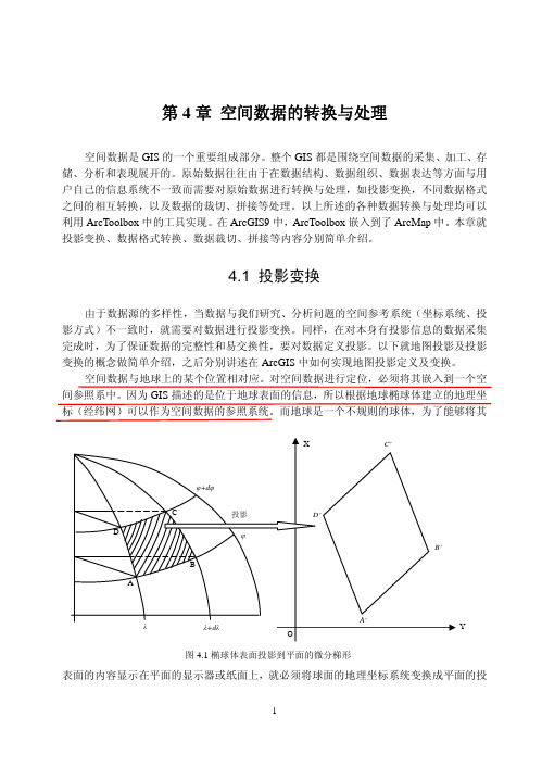
而地球是一个不规则的球体，为了能够将其表面的内容显示在平面的显示器或纸面上，就必须将球面的地理坐标系统变换成平面的投图4.1椭球体表面投影到平面的微分梯形Y影坐标系统（图4.1）。

因此，运用地图投影的方法，建立地球表面和平面上点的函数关系，使地球表面上由地理坐标确定的点，在平面上有一个与它相对应的点。

地图投影的使用保证了空间信息在地域上的联系和完整性。

当系统使用的数据取自不同地图投影的图幅时，需要将一种投影的数字化数据转换为所需要投影的坐标数据。

投影转换的方法可以采用：1. 正解变换: 通过建立一种投影变换为另一种投影的严密或近似的解析关系式，直接由一种投影的数字化坐标x 、y 变换到另一种投影的直角坐标X 、Y 。

有限元等参变换的坐标转换英文回答：Coordinate transformation is an essential concept in finite element analysis. It allows us to express the equations of motion and other physical quantities in different coordinate systems, making it easier to analyze and solve complex problems.In the finite element method, we often work with different coordinate systems, such as global coordinates and local element coordinates. The transformation between these two coordinate systems is known as the isoparametric transformation or the finite element isoparametric mapping.The isoparametric transformation involves mapping the physical domain of an element, defined in global coordinates, to a reference domain, defined in local element coordinates. This mapping is achieved using shape functions, which are mathematical functions that describethe variation of the physical quantities within an element.To illustrate this concept, let's consider a simple example of a 2D beam element. In global coordinates, the beam is defined by its length and orientation. However, in local element coordinates, the beam is defined by its length and orientation relative to the element.When we perform a coordinate transformation, we use shape functions to map the physical coordinates of the element to the reference coordinates. These shape functions are typically polynomials that vary within the element. By applying the shape functions to the physical coordinates, we obtain the corresponding reference coordinates.Once we have the reference coordinates, we can express the physical quantities, such as displacements, strains, and stresses, in terms of the reference coordinates. This allows us to formulate the finite element equations in the reference domain, which simplifies the analysis andsolution process.In addition to the isoparametric transformation, there are other coordinate transformations that are commonly used in finite element analysis. For example, the natural coordinate system is often used to simplify the integration process when evaluating element properties, such as stiffness and mass matrices.Overall, coordinate transformation is a powerful tool in finite element analysis. It allows us to work with different coordinate systems and express physicalquantities in a more convenient and efficient manner. By understanding and applying coordinate transformations, we can effectively analyze and solve complex engineering problems.中文回答：有限元等参变换是有限元分析中的一个重要概念。

三重积分球坐标变换公式雅可比行列式英文版The Jacobian determinant is a key concept in multivariable calculus, particularly when dealing with transformations between coordinate systems. In the context of triple integrals, the Jacobian determinant plays a crucial role in converting integrals from one coordinate system to another.Consider a triple integral in spherical coordinates, where the integrand is a function f(r, θ, φ) and the volume element is given by dV = r^2 sin(φ) dr dθ dφ. To convert this integral to Cartesian coordinates, we need to calculate the Jacobian determinant of the transformation from spherical to Cartesian coordinates.The Jacobian determinant for the transformation from spherical coordinates (r, θ, φ) to Cartesian coordinates (x, y, z) is given by the formula:J = |∂(x, y, z)/∂(r, θ, φ)|To calculate this determinant, we need to find the partial derivatives of x, y, and z with respect to r, θ, and φ. These partial derivatives can be expressed in terms of the unit vectors in each coordinate system:∂x/∂r = sin(φ) cos(θ)∂x/∂θ = -r sin(φ) sin(θ)∂x/∂φ = r cos(φ) cos(θ)∂y/∂r = sin(φ) sin(θ)∂y/∂θ = r sin(φ) cos(θ)∂y/∂φ = r cos(φ) sin(θ)∂z/∂r = cos(φ)∂z/∂θ = 0∂z/∂φ = -r sin(φ)By calculating the determinant of the Jacobian matrix formed by these partial derivatives, we can obtain the Jacobian determinant J. This determinant will then be used to convert the volume element dV = r^2 sin(φ) dr dθ dφ in spherical coordinates to the corresponding volume element in Cartesian coordinates.In summary, the Jacobian determinant is a powerful tool in transforming integrals between different coordinate systems, allowing us to work with a variety of mathematical problems in a more convenient and efficient manner.完整中文翻译雅可比行列式是多元微积分中的一个关键概念，特别是在处理坐标系之间的变换时。

转动惯量坐标系转换公式English Answer:Rotational Inertia Coordinate Transformation Formula.The rotational inertia tensor is a physical quantity that characterizes the resistance of an object to angular acceleration. It is a tensor of rank 2, and its components are defined as the sum of the products of the masses of the particles in the object and the squares of their distances from the axis of rotation.The rotational inertia tensor is a useful quantity for describing the motion of rigid bodies. For example, it can be used to calculate the angular momentum of a body, its kinetic energy, and its moment of inertia.The rotational inertia tensor is also a tensor, which means that it transforms in a specific way under coordinate transformations. The transformation formula for therotational inertia tensor is given by:I' = R I R^T.where:I is the rotational inertia tensor in the original coordinate system.I' is the rotational inertia tensor in the new coordinate system.R is the rotation matrix that transforms the original coordinate system into the new coordinate system.The rotation matrix is a 3x3 matrix that describes the rotation of the original coordinate system into the new coordinate system. The elements of the rotation matrix are the cosines of the angles between the axes of the two coordinate systems.The rotational inertia tensor is a symmetric matrix,which means that it is equal to its transpose. This implies that the transformation formula for the rotational inertia tensor can be simplified to:I' = R I R.The rotational inertia tensor is a useful quantity for describing the motion of rigid bodies. It can be used to calculate the angular momentum of a body, its kinetic energy, and its moment of inertia. The transformation formula for the rotational inertia tensor is given by:I' = R I R^T.where R is the rotation matrix that transforms the original coordinate system into the new coordinate system.Chinese Answer:转动惯量坐标系转换公式。

accreditation 委派accuracy 准确度acquisition 获取activity patterns 活动模式added value 附加值adjacency邻接Aeolian 伊奥利亚人的, 风的, 风蚀的Age of Discovery 发现的年代aggregation聚合algorithm, definition算法,定义ambiguity 不明确analytical cartography 分析制图application programming interfaces(APIs) 应用编程接口ARCGis 美国ESRI公司开发的世界先进的地理信息系统软件ArcIMS 它是个强大的，基于标准的工具，让你快速设计和管理Internet地图服务ArcInfo 在ArcGIS软件家族中，ArcInfo是GIS软件中功能最全面的。

它包含ArcView和ArcEditor 所有功能，并加上高级空间处理和数据转换ArcNews 美国ESRI向用户终生免费赠送的ArcNews报刊ArcSDE ArcSDE在ESRI GIS软件和DBMS之间提供通道，是一个空间数据引擎ArcUser Magazine 为ESRI用户创建的报刊ArcView 桌面GIS和制图软件，提供数据可视化，查询，分析和集成功能，以及创建和编辑地理数据的能力ARPANET ARPA 计算机网（美国国防部高级研究计划局建立的计算机网）aspatial data 非空间数据？Association of Geographic Information (AGI) 地理信息协会attribute data 属性数据attributes, types 属性，类型attributive geographic data 属性地理数据autocorrelation 自相关Autodesk MapGuide 美国Autodesk公司生产的Web GIS软件Automated mapping/facility management(AM/FM) systems 自动绘图/设备管理系统facilities 设备avatars 化身A VIRIS 机载可见光/红外成像光谱仪azimuthal projections 方位投影batch vectorization 批量矢量化beer consumption 啤酒消费benchmarking 基准Berry, Brianbest fit line 最优线binary counting system 二进制计算系统binomial distribution 二项式分布bivariate Gaussian distribution 二元高斯分布block encoding 块编码Bosnia, repartitioning 波斯尼亚，再分离成两个国家buffering 缓冲区分析Borrough, PeterBusiness and service planning(retailing) application in petroleum and convenience shopping 石油和便利购物的业务和服务规划（零售）应用business drivers 业务驱动business, GIS as 业务，地理信息系统作为Buttenfield, Barbaracadasters 土地清册Callingham, Martincannibalizing 调拨Cartesian coordinate system笛卡尔坐标系Cartograms 统计地图cartographic generalization 制图综合cartographic modeling 地图建模cartometric transformations 量图变换catalog view of database 数据库目录视图census data人口普查数据Census of Population 人口普查central Place Theory 中心区位论central point rule 中点规则central tendency 中心倾向centroid 质心choropleth mapping分区制图choosing a GIS 选择一个地理信息系统class 类别classification generalization 分类综合client 客户端client-server C/S结构客户端-服务器cluster analysis 聚类分析clutter 混乱coastline weave 海岸线codified knowledge 编码知识COGO data 坐标几何数据COGO editing tools 坐标几何编辑工具Collaboration 协作Local level 地方级National level 国家级Collection-level metadata 获取级元数据Commercial-off-the-shelf (COTS) systems 成熟的商业化系统chemas-microsoft-comfficeffice" />>> Commom object request broker architecture (CORBA) 公共对象请求代理体系结构Community, GIS 社区，地理信息系统Competition 竞争Component GIS 组件地理信息系统Component object model (COM) 组件对象模型Computer assisted mass appraisal (CAMA) 辅助大量估价，>>Computer-aided design (CAD)-based GIS 基于计算机辅助制图的地理信息系统Models 数据模型Computer-aided software engineering (CASE) tool 计算机辅助软件工程工具Concatenation 串联Confidence limits 置信界限Conflation 异文合并Conformal property 等角特性Confusion matrix 混淆矩阵Conic projections 圆锥投影Connectivity 连接性Consolidation 巩固Constant term 常数项Contagious diffusion 传染扩散Continuing professional development (CPD) 持续专业发展Coordinates 坐标Copyright 版权Corridor 走廊Cost-benefit analysis 成本效益分析Cost-effectiveness evaluation 成本效率评估Counting method 计算方法Cresswell, PaulCustomer support 客户支持Cylindrical Equidistant Projection 圆柱等距投影Cylindrical projections 圆柱投影> >Dangermond, Jack 美国ESRI总裁>> dasymetric mapping 分区密度制图>>data 数据>>automation 自动化>>capture costs 获取代价>>capture project 获取工程>>collection workflow 采集工作流>> compression 压缩>>conversion 转换>>definition 定义>>geographic, nature of 地理数据，数据的性质>> GIS 地理信息系统>>industry 产业>>integration 集成>>mining 挖掘>>transfer 迁移>>translation 转化>>data model 数据模型>> definition 定义>>levels of abstraction 提取等级>> in practice 实际上>>types 类型>>database 数据库>>definition 定义>>design 设计>>generalization 综合>>global 全球的>>index 索引>>multi-user editing 多用户编辑>> structuring 结构>>database management system (DBMS) 数据库管理系统>>capabilities 能力>>data storage 数据存储>>geographic extensions 地理扩展>>types 类型>>Dayton Accord 达顿协定，1995年12月达顿协定(DAYTON ACCORD)签订,巴尔干和平已经实现,波斯尼亚(包括黑塞哥维那)再被分解成两个国家>>decision support 决策支持>>deductive reasoning 演绎推理>>definitions of GIS 地理信息系统的各种定义>>degrees of freedom 自由度>>density estimation 密度估算>>dependence in space 空间依赖>>desktop GIS 桌面地理信息系统>>desktop paradigms 桌面范例>>Digital Chart of the World (DCW) 世界数字化图>>digital divide 数字鸿沟>>Digital Earth 数字地球>>Digital elevation models (DEMs) 数字高程模型>>Digital line graph (DLG) 数字线划图>>Digital raster graphic (DRG) 数字影像图>>Digital representation 数字表现>>Digital terrain models 数字地形模型>>Digitizing 数字化>>DIME (Dual Independent Map Encoding) program 美国人口调查局建立的双重独立地图编码系统>> Dine CARE >>Discrete objects 离散对象>>Douglas-Poiker algorithm 道格拉斯-普克算法，一种矢量数据抽稀算法>>Dublin Core metadata standard 都柏林核心元数据标准>>Dynamic segmentation 动态分割>>Dynamic simulation models 动态仿真模型>>> >Easting 朝东方>>Ecological fallacy 生态谬误>>e-commerce 电子商业>>editing 编辑>>education 教育>>electromagnetic spectrum 电磁光谱>>ellipsoids 偏振光椭圆率测量仪>>of rotation 旋转的>>emergency evacuation 应急撤退>>encapsulation 封装>>environmental applications 环境应用>>environmental impact 环境影响>>epidemiology 流行病学>>equal area property 等面积特性>>Equator 赤道>>ERDAS ERDAS公司是世界上最大的专业遥感图像处理软件公司，用户遍布100多个国家，软件套数超过17000套。

ADINA中的坐标系（轴）及其用途、用法――ADINA广州王学超坐标系（轴）是ADINA中最基本的内容，在建模、初始/边界条件施加及结果后处理中都起着重要的作用，是学习和精通ADINA所必须完全掌握的重要方面。

由于ADINA的坐标系（轴）涉及到的内容较为广泛，有必要对ADINA的坐标系（轴）加以归纳整理。

ADINA中的坐标系（轴）主要有以下9种：Global System（整体坐标系）Local Coordinate System（局部坐标系）Skew System（斜坐标系）Geometry Triads（几何的坐标架）Element Local Coordinate System（单元坐标系）Orthotropic Axes System（用于与初始应变轴或材料轴对齐的正交轴系）Initial Strain Axes（初始应变轴）Material Axes（材料轴）Result Transformation System（结果转换坐标系）下面将分别对上述的9种坐标系进行详细的介绍。

1、Global System（整体坐标系）说明：整体坐标系在ADINA中已经默认存在，如图1.1所示，不需要用户自行定义，也不能改动，其坐标系的名称代号为0。

用途：可用于ADINA建模、求解及后处理的所有过程，默认情况下，ADINA所有的建模、求解及后处理的所有结果都可以基于该坐标系。

另外，ADINA的求解过程也只能在整体坐标系中进行，所有基于其他坐标系的边界、载荷等信息求解时将会自动转换到整体坐标系。

图1.1注意：后处理中，标有X、Y、Z或XX、YY、ZZ、XY、XZ、YZ的结果一般都是基于整体坐标系的结果，但对于3-D plane stress类型的单元，标有YY、ZZ等的结果为单元坐标系的结果，具体可参看理论手册。

2、Local Coordinate System（局部坐标系）说明：局部坐标系需要用户自行定义，有直角坐标、柱坐标、球坐标三种类型。

体数据任意角度切面计算原理英文版Volume Data Arbitrary Angle Section Calculation Principle In the realm of computer graphics, 3D modeling, and medical imaging, the calculation of arbitrary angle sections of volumetric data is crucial for accurate visualization, analysis, and manipulation of 3D objects or structures. This article aims to explain the principles behind the computation of such sections, commonly referred to as "slicing" or "clipping" in technical parlance.Principles of Volumetric Data SectioningVolumetric data, essentially, is a representation of a three-dimensional object or structure in digital form. It typically consists of a grid of voxels (volume pixels), each carrying information about a specific point in space. To calculate a section at an arbitrary angle, we need to consider the geometry and data structure of the volumetric data.Coordinate Systems and Transformations: The first step is to define the coordinate system in which the volumetric data resides. This is usually a 3D Cartesian coordinate system. To obtain a section at an arbitrary angle, we need to apply affine transformations to the coordinate system. These transformations involve rotations, translations, and possibly scaling, depending on the desired orientation of the section plane.Section Plane Definition: The next step is to define the section plane. This plane is described by its normal vector and a point on the plane. The normal vector determines the orientation of the plane, while the point defines its position in space. By adjusting these parameters, we can obtain sections at different angles and positions.Voxel-Plane Intersection: Once the section plane is defined, we need to determine which voxels intersect with this plane. This involves performing ray-box intersection tests for eachvoxel against the section plane. The voxels that intersect with the plane are considered part of the section.Interpolation and Sampling: Since the section plane may not align exactly with the voxel grid, interpolation is often required to obtain accurate values at the intersection points. This involves sampling the voxel data along the intersection line and computing a weighted average based on the fractional part of the intersection coordinate.Section Image Generation: Finally, the intersection points are combined to form the final section image. This image represents a 2D projection of the volumetric data along the defined section plane. It can be displayed, analyzed, or further processed as needed.ConclusionThe calculation of arbitrary angle sections of volumetric data involves several key steps, including coordinate system transformations, section plane definition, voxel-plane intersection testing, interpolation, and section image generation.Understanding these principles is crucial for effective manipulation and visualization of 3D data in various applications such as medical imaging, computer graphics, and scientific visualization.中文版体数据任意角度切面计算原理在计算机图形学、3D建模和医学成像领域，体数据的任意角度切面计算对于3D对象或结构的准确可视化、分析和处理至关重要。

Package‘PROJ’December1,2023Title Generic Coordinate System Transformations Using'PROJ'Version0.4.5Description A wrapper around the generic coordinate transformation software'PROJ' that transforms coordinates from one coordinate reference system('CRS')to another.This includes cartographic projections as well as geodetic transformations.The in-tention is for thispackage to be used by user-packages such as'reproj',and that the older'PROJ.4'and version5 pathways be provided by the'proj4'package.Depends R(>=3.0.2)License GPL-3Encoding UTF-8LazyData trueSuggests testthat(>=2.1.0),spelling,knitr,rmarkdownURL https:///hypertidy/PROJBugReports https:///hypertidy/PROJ/issuesLanguage en-USVignetteBuilder knitrSystemRequirements PROJ(>=6.3.1)RoxygenNote7.2.3NeedsCompilation yesAuthor Michael D.Sumner[aut,cre](<https:///0000-0002-2471-7511>), Jeroen Ooms[ctb](provided PROJ library support on Windows,andassistance with Windows configuration),Simon Urbanek[cph,ctb](wrote original code versions for PROJ version6),Dewey Dunnington[ctb](key code contributions)Maintainer Michael D.Sumner<******************>Repository CRANDate/Publication2023-12-0122:10:08UTC12ok_proj6 R topics documented:ok_proj6 (2)proj_crs_text (3)proj_trans (4)proj_version (5)xymap (5)Index6 ok_proj6Is’PROJ library>=6’availableDescriptionTest for availability of’PROJ’system library version6or higher.Usageok_proj6()DetailsOn unix-alikes,this function is run in.onLoad()to check that version6functionality is available.On Windows,the load process sets the datafile location with the version6API,and that is used asa test instead.If’PROJ’library version6is not available,the package still compiles and installs but is not func-tional.The lack of function can be simulated by setting options(reproj.mock.noproj6=TRUE),de-signed for use with the reproj package.Valuelogical,TRUE if the system library’PROJ>=6’Examplesok_proj6()proj_crs_text3 proj_crs_text Generate a projection string.DescriptionInput any accepted format of’PROJ’coordinate reference system specification.Return value is a string in the requested format.Usageproj_crs_text(source,format=0L)Argumentssource input projection specification one of(’PROJ4’,’WKT2’,’EPSG’,’PROJJSON’, ...see the library documentation link in Details)format integer,0for’WKT’,1for’PROJ’,2for’PROJJSON’DetailsThis function requires PROJ version6.0or higher to be useful.If not,this function simply returns ’NA’.See the library documentation for details on input and output formats.Valuecharacter string in requested formatwarning Note that a PROJ string is not a full specification,in particular this means that a string like "+proj=laea"cannot be converted to full WKT,because it is technically a transformation step not a crs.To get the full WKT form use a string like"+proj=laea+type=crs".Examplesif(ok_proj6()){cat(proj_crs_text("OGC:CRS84",format=0L))proj_crs_text("OGC:CRS84",format=1L)south55<-"+proj=utm+zone=55+south+ellps=GRS80+units=m+no_defs+type=crs"proj_crs_text(proj_crs_text(south55),1L)}4proj_trans proj_trans Transform a set of coordinates with’PROJ’DescriptionA raw interface to’proj_trans’in’PROJ=>6’,if it is available.Usageproj_trans(x,target,...,source=NULL,z_=NULL,t_=NULL)Argumentsx input coordinates(x,y,list or matrix see z_and t_)target projection for output coordinates...ignoredsource projection of input coordinates(must be named i.e.’source="<some proj string"’can’t be used in positional form)z_optional z coordinate vectort_optional t coordinate vectorDetailsInput’x’is assumed to be2-columns of"x",then"y"coordinates.If"z"or"t"is required pass these in as named vectors with"z_"and"t_".For simplifying reasons z_and t_must always match the length of x y.Both default to0,and are automatically recycled to the number of rows in x.Values that are detected out of bounds by library PROJ are allowed,we return Inf in this case, rather than the error"tolerance condition error".Valuelist of transformed coordinates,with4-or2-elements x_,y_,z_,t_Referencessee the PROJ library documentation for details on the underlying functionalityExamplesif(ok_proj6()){proj_trans(cbind(147,-42),"+proj=laea",source="OGC:CRS84")proj_trans(cbind(147,-42),z_=-2,"+proj=laea",source="OGC:CRS84")proj_trans(cbind(147,-42),z_=-2,t_=1,"+proj=laea",source="OGC:CRS84")}proj_version5 proj_version Report PROJ library versionDescriptionThis function returns NA if PROJ lib is not available.Usageproj_version()Valuecharacter string(major.minor.patch)Examplesproj_version()xymap xymap data for testingDescriptionA copy of the xymap data set from the quadmesh package.DetailsA matrix of longitude/latitude values of the world coastline.Indexok_proj6,2proj_crs_text,3proj_trans,4proj_version,5xymap,56。

三维激光扫描坐标系转换方法Three-dimensional laser scanning is a widely used technology in fields such as engineering, architecture, and archaeology. It allows for the accurate and detailed capture of physical objects and their surrounding environments. However, the data collected from a three-dimensional laser scan is often captured in a specific coordinate system, and it may be necessary to convert this data to a different coordinate system for further analysis or integration with other data sources.三维激光扫描技术在工程、建筑和考古等领域被广泛应用。

它可以准确、详细地捕捉物体及其周围环境的数据。

然而，从三维激光扫描中收集的数据通常是在特定的坐标系统中获取的，可能需要将这些数据转换为不同的坐标系统进行进一步分析或与其他数据源集成。

One method for converting the coordinate system of three-dimensional laser scan data is through the use of transformation matrices. A transformation matrix is a mathematical tool that allows for the conversion of coordinates from one system to another. It involves using a combination of translation, rotation, and scaling tomap the points from the original coordinate system to the new one. This method is widely used in computer graphics and computer-aided design, and it can be applied to three-dimensional laser scan data to achieve the desired coordinate system transformation.一种转换三维激光扫描数据坐标系的方法是使用转换矩阵。

EX03：ArcGIS中的坐标系统及其转换本次实验包含3个任务。

任务1是将一个shapefile由Geographic coordinate system（地理坐标系统）投影（Project）到用户自定义的Project coordinate system（投影坐标系统）。

任务2同样与1大致相同，其间需要使用任务1定义的坐标系统。

任务3是由一个包含点位地理坐标的文本文件创建shapefile，并且将它投影到ArcGIS系统中预定义的投影坐标系统。

任务1：将一个Feature Class由地理坐标系统投影到投影坐标系统所需数据：idll.shp，一个以十进制度表示经纬度数值的shapefile，为Idaho州的轮廓图。

在任务1中，将idll.shp投影到Idaho州横轴麦卡托（Idaho Transverse Mercator, IDTM）坐标系统，因为IDTM不是一个预定义系统，则首先要对IDTM坐标系统进行定义，IDTM 参数设置如下：Projection Transverse MercatorDatum NAD83Units metersParametersscale factor: 0.9996central meridian: -114.0reference latitude: 42.0false easting: 2,500,000false northing: 1,200,0001.启动ArcCatalog，连接到EX03数据所在文件夹，在Catalog中选择idll.shp，在Metadata页中，单击Spatial，显示其坐标系统归为地理（Geographic）坐标系统，名称为GCS_Assumed_Geographic_1，一个假定的坐标系统（图3.1）。

图3.1 图层的空间参考信息2.首先要定义需要的坐标系统（图3.2）。

在ArcCatalog中打开ArcToolbox窗口，右键单击ArcToolbox选择Environments（环境），将EX03数据所在文件夹设置为当前工作空间（Workspace Space）。

ArcGIS教程：为shape文件设置投影为了使river shape文件与GreenvalleyDB地理数据库中的数据有相同的坐标系，那么要对shape文件的投影进行设置，设置shape文件有两个步骤：首先必须为shape文件定义一个坐标系，然后定义输出坐标系和投影文件。

可以用ArcToolbox来实现，它包含许多数据管理和转换的工具盒向导。

为river shape文件定义坐标系1.ArcCatalog中，单击工具条中的Show/Hide ArcToolbox按钮，ArcToolbox窗口弹出。

2. 双击ArcToolbox目录树中的Data Management Tools;双击Projections and Transformations，然后再双击Define Projection工具。

如果使用ArcInfo，将不能看到其余的工具。

Define Projection对话框弹出。

在ArcCatalog中用Properties对话框为lowland shape文件定义坐标系，ArcToolbox是定义坐标系的一个方法。

3. 单击Input Dataset或者Feature Class browse按钮，找到project文件夹里的County_share文件夹。

4. 选中river.shp，然后单击Add。

向导列出了shape文件，坐标系统是GCS_Assumed_Geographic_1。

ArcGIS将根据数据集的坐标值来决定shape文件的坐标系统。

在本例中，ArcGIS已经确定了shape文件是地理坐标系(经度和纬度)中，而通常在开始投影数据前必须明确定义坐标系统。

5.单击Coordinate System旁边的按钮。

Spatial Reference Properties对话框弹出。

有三种方法定义坐标系：使用保存在.prj文件中预定义好标系;通过确定一个数据集的名字配准的现有数据集的坐标系;或根据投影、基准面和相关参数的相互关系确定坐标系。

大地坐标和北京54等坐标系之间的转换The transformation between geodetic coordinate and Beijing 54 Coordinate SystemCoordinate transformation between different coordinate systems is often encountered in the process of Engineering construction. At present, there are several common transformations in China: 1. Geodetic coordinate (BLH) to plane Cartesian coordinates (XYZ); 2, Beijing 54, national 80 and WGS84 coordinate systems; 3, conversion of any two space coordinate system. Second of these categories fall into the third category. The process of coordinate transformation is the process of solving the transformation of parameters. The common methods include three parameter method, four parameter method and seven parameter method. The following three cases are described in detail below:1, the geodetic coordinate (BLH) pair of plane Cartesian coordinates (XYZ)Conventional transformations should first determine conversion parameters, namely ellipsoid parameters, zonation criteria (3 degrees, 6 degrees), and longitude of the central meridian. The ellipsoid parameter refers to Cartesian coordinates with the ellipsoid reference what, there are different length axis and flattening. In general engineering, 3 degree belt is widely used. There are two ways to determine the central meridian. First, take the first two *3 of the Y coordinate in the plane Cartesian coordinate system, and then get the longitude of the corresponding central meridian. For example, x=3250212m, y=395121123m, the longitude of thecentral meridian is =39*3=117 degrees. Another method is based on geodetic coordinates, longitude, and if the longitude is between 155.5~185.5 degrees, then the longitude of the corresponding central meridian = (155.5+185.5) /2=117 degrees, and the rest can be based on 3 degrees of analogy.In addition, some projects use their own special zoning standards, and the corresponding parameters are not listed in the above column.After you have determined the parameters, you can convert them with software. The following programs that provide coordinate conversion are downloaded.2, the transformation of the 80 and WGS84 coordinate systems of Beijing 54These three coordinate systems are commonly used in China, and they adopt different ellipsoid datum.The 54 Beijing coordinate system, three coordinate system, the origin of the earth in the Soviet Union and general coward, the long axis 6378245m, short axis of 6356863, 1/298.3; Xi'an 80 coordinate system, three coordinate system, the origin of the earth in Shaanxi province Jingyang County Yongle Town, long axis 6378140m, short axis 6356755, of 1/298.25722101; WGS84 coordinate axis, short axis 6378137.000m, 6356752.314, of1/298.257223563. Due to the different ellipsoid standards, and due to the limitations of projection, there is no one to all conversion parameters throughout the country. For this conversion due to the large amount of conditions, generally usemultiple GPS known point, coordinate conversion automatically using GPS software. Of course, if the condition does not permit and has enough coincidence point, may also carry on the artificial solution. See the third class for details.3, the transformation of any two space coordinate systemSince the measurement coordinate system and the construction coordinate system use different standards for accurate conversion, it is necessary to know at least 3 coincidence points (i.e., the coordinates in the two coordinate system are known points. The Boolean model is used to solve the problem. Boolean formula:The formula is transformed equivalently:To solve these seven parameters, we need to use at least three known points (coordinate of 2 coordinate systems),The indirect adjustment model is used to solve the problem:Where: V is the residual matrix;X is an unknown seven parameter;A is the coefficient matrix;Solution: L is the closure differenceThe seven parameter solution, using Boolean formula can Shakespeare unknown coordinate conversion, each input a set ofcoordinates, it can be calculated in the new coordinate system in the coordinates. But in order for GPS observations to be used for engineering or mapping, local Cartesian coordinates need to be converted to geodetic coordinates, and eventually converted to plane Gauss coordinates.This method is similar to the indirect adjustment, the solution is complicated, the coordinate conversion program, simply enter the three known point coordinates can be calculated seven parameters of coordinate transformation. If the number of known points is more, the adjustment between parameters can be carried out, and then the accuracy is higher.When the number of known points is only two, we can adopt the simple transformation method. This method is more convenient and suitable for hand calculation, but the accuracy is limited.The detailed solution equations are as follows:The central modulation x, y and x\', y\' are the coordinates of the coincidence points of the old (or the old) network, a, B, and K are the transformation parameters, and it is obvious that a, B, and K must be solved at least two coincidence points, and four equations are listed.The common parameter adjustment can be carried out, and the parameters of a, x, B, C and D are solved. The generation of (3) formula, you can get the residuals of each fitting point (modified), the generation (2) formula, you can get the coordinates of the change point.After calculating the parameters, the transformation of the rest of the coordinates can be done in Excel.Last time I used this method for 80 and 54 Coordinate conversion, because there was no excess points for verification of peace difference, so the conversion accuracy is unknown, but the relative positions of the points after the conversion remain unchanged. It is estimated that the actual conversion error should be 10m orders of magnitude.In other cases, the geodetic coordinates are converted into Cartesian coordinates, and then related transformations are made.。