
第八章Simulink 基础
Chapter 8: Introduction to Simulink
一.Simulink 初步(Primer of Simulink)
MATLAB Simulink是一个动态仿真系统,用于对动态系统进行仿真和分析,预先模拟实际系统的特性和响应,根据设计和使用要求,对系统进行修改和优化。
Simulink提供了图形化用户界面,只须点击鼠标就可以轻易的完成模型的创建、调试和仿真工作,用户不须专门掌握一种程序设计语言。
Simulink可将系统分为从高级到低级的几个层次,每层又可以细分为几个部分,每层系统构建完成后,将各层连接起来就可构成一个完整的系统。
模型创建完成后,可以启动系统的仿真功能分析系统的动态特性,其内置的分析工具包括各种仿真算法、系统线性化、寻求平衡点等。仿真结果可以以图形方式在示波器窗口显示,也可将输出结果以变量形式保存起来,并输入到MATLAB中以完成进一步的分析。
Simulink可以仿真线性和非线性系统,并能创建连续时间、离散时间或二者混合的系统。支持多采样频率系统。
Simulink:Version 6.0 (R14) 05-May-2004
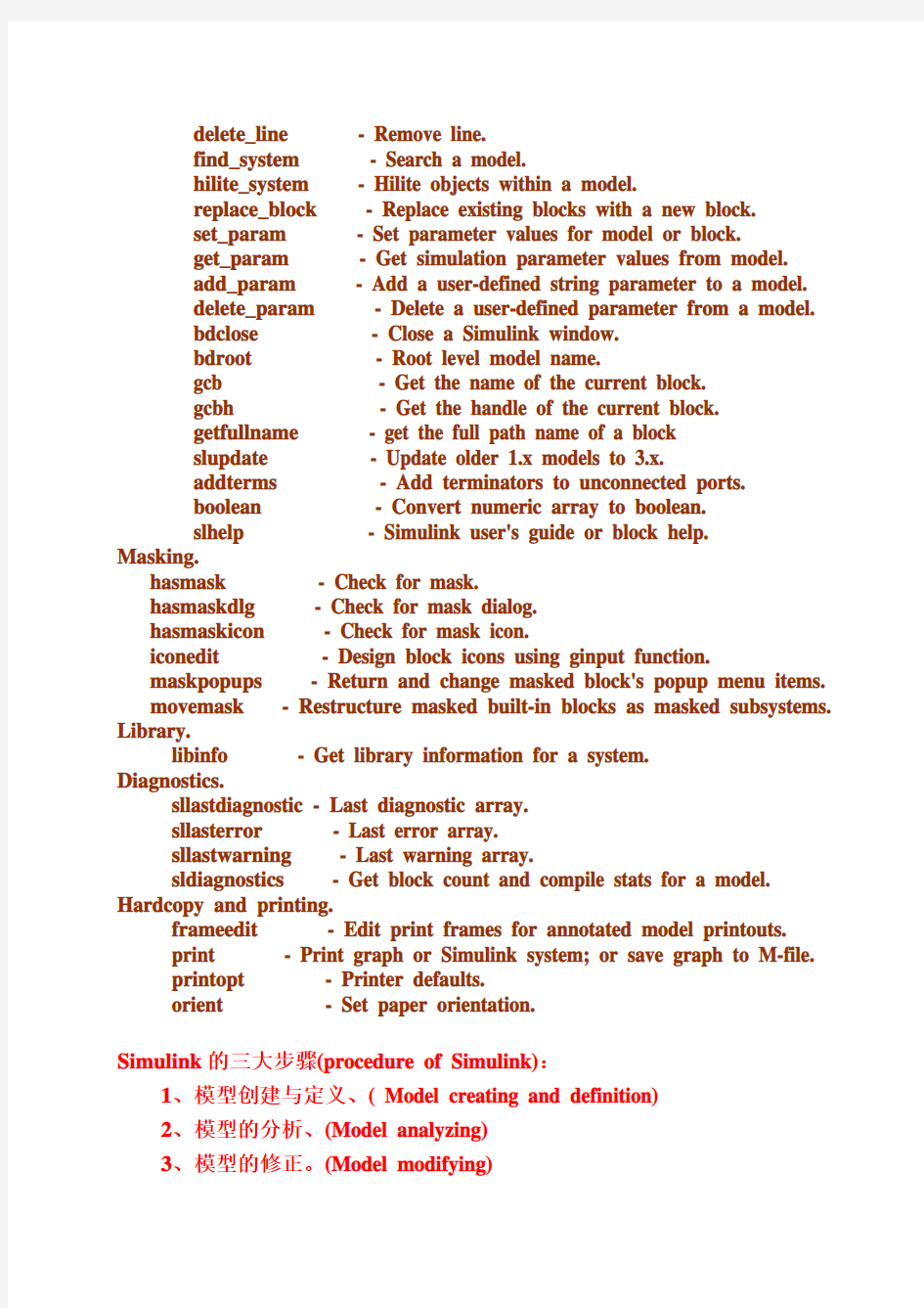
Model analysis and construction functions.
Simulation
sim - Simulate a Simulink model.
sldebug - Debug a Simulink model.
simset - Define options to SIM Options structure.
imget - Get SIM Options structure Linearization and trimming.
linmod - Extract linear model from continuous-time system.
linmo - Extract linear model, advanced method.
dlinm - Extract linear model from discrete-time system.
trim - Find steady-state operating point.
Model Construction.
close_system - Close open model or block.
new_system - Create new empty model window.
open_system - Open existing model or block.
load_system - Load existing model without making model visible.
save_system - Save an open model.
add_block - Add new block.
add_line - Add new line.
delete_block - Remove block.
delete_line - Remove line.
find_system - Search a model.
hilite_system - Hilite objects within a model.
replace_block - Replace existing blocks with a new block.
set_param - Set parameter values for model or block.
get_param - Get simulation parameter values from model.
add_param - Add a user-defined string parameter to a model.
delete_param - Delete a user-defined parameter from a model.
bdclose - Close a Simulink window.
bdroot - Root level model name.
gcb - Get the name of the current block.
gcbh - Get the handle of the current block.
getfullname - get the full path name of a block
slupdate - Update older 1.x models to 3.x.
addterms - Add terminators to unconnected ports.
boolean - Convert numeric array to boolean.
slhelp - Simulink user's guide or block help.
Masking.
hasmask - Check for mask.
hasmaskdlg - Check for mask dialog.
hasmaskicon - Check for mask icon.
iconedit - Design block icons using ginput function.
maskpopups - Return and change masked block's popup menu items.
movemask - Restructure masked built-in blocks as masked subsystems. Library.
libinfo - Get library information for a system.
Diagnostics.
sllastdiagnostic - Last diagnostic array.
sllasterror - Last error array.
sllastwarning - Last warning array.
sldiagnostics - Get block count and compile stats for a model. Hardcopy and printing.
frameedit - Edit print frames for annotated model printouts.
print - Print graph or Simulink system; or save graph to M-file.
printopt - Printer defaults.
orient - Set paper orientation.
Simulink的三大步骤(procedure of Simulink):
1、模型创建与定义、( Model creating and definition)
2、模型的分析、(Model analyzing)
3、模型的修正。(Model modifying)
如下图所示,重复执行上述三大步骤可以实现系统的最优化。
Simulink的运行:(Running of Simulink)
1、运行Simulink:命令窗口下点击Simulink图标(或在命令窗口键入
Simulink命令)→Sim(浏览器)→sim
树状列表形式的模块库(包含simulink模块库中的各种模块及其它Toolbox和Blockset中的模块)
2、选择建模模块:展开树状列表,用鼠标点击所需类别的模块项,所
选模块类的具体模块库就在右侧的列表框中显示出来,提供建模使用。
也可以在输入栏中键入模块名并点击Find按钮进行查询。
3、打开模型创建窗口:(open the window of mode creating)。
在工具栏中选择“建立新模型”的图标,弹出名为Untitled的空白窗口,选择Open窗口可以打开存于硬盘中已建的模型,完成模型的运行或修改。
二.Simulink 的常用基本模块(basic module)
simulink浏览器窗口左侧的simulink项上单击鼠标右键,弹出菜单“Open the …Simulink?Labrary’”选项,将打开simulink模块库窗口。常用的模块主要为:
1.信号源模块:source,模块及功能见(表8—1)
2.输出模块:Sinks, 模块及功能见(表8—2)
3. 连续系统模块:Continuous, 模块及功能见(表8—3)
4. 离散系统模块:Discrete, 模块及功能见(表8—4)
5. 数学运算模块:Math, 模块及功能见(表8—5)
6.函数和表模块:Function & Tables, 模块及功能见(表8—6)
7. 非线性系统模块:Nonlinear, 模块及功能见(表8—7)
8. 信号与系统模块:Signal & Systems, 模块及功能见(表8—8)还有:
常用模块:Commonly used blocks
非连续模块:Discontinuous
逻辑运算和二进制数位模块:Logical and bit operation
插值表:Lookup tables
模式识别Model:Verification
端口及子系统:Ports and subsystems
用户自定义函数:User defined functions
辅助数学和离散系统:Additional math and discrete
可选示波器(Floating scope):可在示波器窗口的Floating scope快捷键将普通示波器转变为Floating scope,也可在模型库中直接选择Floating scope模块。利用Floating scope模块可选择显示一或多个线程上的信号,模块不必与模型中的信号线连接,可以在signal selection 快捷键打开的菜单中选择要显示的信号。
*Floating scope:
This option appears only on the General parameters pane for the Scope block. Selecting this option turns a Scope block into a floating scope. A floating scope is a Scope block that can display the signals carried on one or more lines. You can create a Floating Scope block in a model either by copying a Scope block from the Simulink Sinks library into a model and selecting this option or, more simply, by copying the Floating Scope block from the Sinks library into the model window. The Floating Scope block has the Floating scope parameter selected by default. To use a floating scope during a simulation, first open the scope. To display the signals carried on a line, select the line. Hold down the Shift key while clicking another line to select multiple lines. It might be necessary to click the Autoscale data button on the floating scope's toolbar to find the signal and adjust the axes to the signal values. Or you can use the floating scope's Signal Selector (see The Signal Selector in the online Simulink documentation) to select signals for display. To display a floating scope's Signal Selector, first start simulation of your model with the floating scope open. Then right-click your mouse in the floating scope and select Signal Selection from the pop-up menu that appears. You can have more than one floating scope in a model, but only one set of axes in one scope can be active at a given time. Active floating scopes show the active axes by making them blue. Selecting or deselecting lines affects the active floating scope only. Other floating scopes continue to display the
signals that you selected when they were active. In other words, inactive floating scopes are locked, in that their signal displays cannot change. To specify display of a signal on one of the axes of a multiaxis floating scope, click the axis. Simulink draws a blue border around the axis. Then click the signal you want to display in the block diagram or the Signal Selector. When you run the model, the selected signal appears in the selected axis. If you plan to use a floating scope during a simulation, you should disable signal storage reuse. See "Signal storage reuse" in Optimizations for more information
三. Simulink 建模(Simulinc module creating)
1.模块的创建与操作(Creating and operation of Simulink)
(1) 创建模块:(module creating)
(1)在浏览器列表中点击需要的模块,按住鼠标左键并拖曳至模型窗口即可。
(2)双击模块可在弹出的对话框中修改相应的模块参数
(3)在模块下方名称处双击可改变模块名称。
(2)模块操作(module operation)
(a)模块的选择(module selection)
(b)移动模块(module moving)
(c)模块的缩放(modulee scaling)
(d)复制模块:(module copy)
四种方法:
*在选定模块处,按下鼠标右键并拖动至适当位置;
*选定模块,在工具栏中(或Edit菜单中)选中Copy与Paste按钮;
*在选定的模块处点击鼠标右键,在弹出的菜单中选择Copy与Paste选项;
*按住”Ctr l”键,按下鼠标左键,将选定的模块拖至适当的位置。
(e)模块的旋转与翻转:(Rotating and turnover of module)
旋转:(rotate)将鼠标指向要翻转的模块并按下鼠标右键,选择弹出菜单中的Format栏中的Rotate项,模块顺时针旋转90o。
翻转:将鼠标指向要翻转的模块并按下鼠标右键,选择弹出菜单中的Format栏中的Flip Block项,模块顺时针旋转180o。
(f)模块的连接
(h)连接分支线
(i)改变连线的形状
(j)连线的标识:在连线的上或下方(或窗口内任何位置)双击鼠标左
键,可出现一个文本框用于输入说明文字。(3).简单模型(Simple mode)
信号发生器发生幅值为1,频率为0.2HZ的正弦波信号,信号分别按1倍和5倍送入两个示波器。
2.模型的修饰(Mode modifying)
1.模块加阴影:Format菜单中的Show drop shadow菜单项用于给
模块加阴影。
2.调整颜色:Format菜单中的Foreground color菜单项用于调整模
块的前景颜色。Background color菜单项用于选择模块的背景颜
色。Screen color菜单项用于调整屏幕颜色。
3.变换模块名的显示位置:Format 菜单中的Flip name可将模块
名换到对称的位置,Hide name可将模块名隐藏起来。
4. 模块修饰的一个简单示例
三.模型中的子系统
把模型中的摹写某些模块组合在一起形成独立的子系统,在主系统中以子系统模块加入,其作用相当于MATLAB指令运行中的M函数文件。
建立子系统的好处:
a, 减少主系统显示在窗口中的模块数目;
b, 将功能相关的模块组合在一起,实现进一步模块化的要求;
c, 构成一个层次分明的大系统。
一)子系统的建立
1)、在模型窗口中添加一个subsystem子块,然后把该模块包含的模块添加进去即可;
2)若组成一个子系统的模块已经添加进去,就将这些模块归入一个子系统中。
1、在subsystem模块建立子系统
*在Simulink Library Browser中打开Simulingk库,从其中的
Ports$Subsystems 库中选取合适的Subsystem拖至模型窗口中。
*双击Subsystem模块,打开Subsystem窗口;
*将要组合的模块拖至Subsysytem窗口中,然后在该窗口中加入Input模块表示从子系统外部到内部的输入,加入Output模块表示从子系统内部到外部的输出,将这些模块按顺序连接起来,子系统便建立成功了。
例:
2、组合已有的模块建立子系统
如欲将已有的模块群变成子系统,操作较简单,步骤为:
*用鼠标划定方框同时选中待组合的模块或按住shift键逐个选中;
*选择EditCreate --Subsystem菜单或单击鼠标右键,在弹出菜单中选择CreateSubsystem ,子系统就建成了。
例:
3、条件执行子系统
由某个外部的决定条件确定是否执行的子系统,由输入的控制信号来控制。常用的条件执行子系统为:
1)使能子系统(Enable Subsystem)
使能子系统在控制信号从负数朝正向穿过零时开始执行,直到控制信号变为负数时停止。
使能子系统在外观上一有一个“使能”控制信号输入口。当且仅当“使能”信号输入口信号为正时,该模块开始接受In输入口端的信号。
使能子系统包括任何连续和离散的模块。
例:
2) 触发子系统(Trigger Subsystem)
触发子系统是指当触发事件发生时开始执行的子系统。在它的外观上有一个“触发”控制信号输入口,仅当触发输入信号所定义的某个事件恰巧发生时,该模块才开始接受In输入端的信号。子系统一旦触发,其输出端口的值就保持不变,直到下次再触发才可能改变。
“触发事件”由子系统内触发模块对话框定义,有4种触发事件可供选择:*rising 上升沿触发
*falling 下降沿触发
*either 任意沿触发
*function-call 函数调用触发
注:一般的连续时间模块不能置于触发子系统中。
例:利用触发子系统获取零阶保持的采样信号实例
1)构造一个仿真模型,保存为test2
2)设置模块参数:Pulse Generator: Amplitude 为1,Period
为1,Pulse Width为50, Phase delay为0;
Sine Wave: Amplitude为1,Frequency为1, Phase为0,
Start time为0
3)在MATLAB命令窗口中运行Simulink模型, 该模型被保存在MATLAB搜索路径上,在命令窗口中运行如下命令:[t,x,y]=sim('test2',10); %调用test2
clf,
hold on
plot(t,y(:,1),'b')
stairs(t,y(:,2),'r')
stairs(t,y(:,3),'g')
hold off
axis([0 10 -1.1 1.1]),box on
legend('正弦波','输出','三角形',4)
运行后即可输出结果.
SIM: Simulate a Simulink model
SimOut = SIM('MODEL', PARAMETERS) simulates your Simulink model, where
'PARAMETERS' represents a list of parameter name-value pairs, a structure
containing parameter settings, or a configuration set. The SimOut returned by the
SIM command is an object that contains all of the logged simulation results. Optional PARAMETERS can be used to override existing block diagram configuration parameters
for the duration of the simulation.
This syntax is referred to as the 'Single-Output Format'.
SINGLE-OUTPUT FORMAT
SimOut = SIM('MODEL','PARAMETER_NAME1',VALUE1,'PARAMETER_NAME2',VALUE2, ...)
SimOut = SIM('MODEL', PARAM_NAME_VAL_STRUCT)
SimOut = SIM('MODEL', CONFIGSET)
All simulation outputs (logged time, states, and signals) are returned in a
single Simulink.SimulationOutput object. Using the model's Configuration Parameters Data Import/Export dialog, you define the model time, states, and
output to be logged. You can log signals using blocks such as the
To Workspace and Scope blocks. The Signal & Scope Manager can directly log signals.
Where:
SimOut : Returned Simulink.SimulationOutput object containing all of the simulation output.
'MODEL' : Name of a block diagram model.
'PARAMETER_NAMEk': Name of the Configuration or Block Diagram parameter.
VALUEk : Value of the corresponding Configuration or Block Diagram parameter.
PARAM_NAME_VAL_STRUCT : This is a structure whose fields are the names
of the block diagram or the configuration parameters that are being changed
for the simulation. The corresponding values are the corresponding parameter
values.
CONFIGSET : The set of configuration parameters for a model.
The single-output format makes the SIM command compatible with PARFOR
by eliminating any transparency issues. See "Running Parallel
Simulations" in the Simulink documentation for further details.
Example 1:
simOut = sim('vdp','SimulationMode','rapid','AbsTol','1e-5',...
'SaveState','on','StateSaveName','xoutNew',...
'SaveOutput','on','OutputSaveName','youtNew');
simOutVars = simOut.who;
yout = simOut.find('youtNew');
Example 2:
paramNameValStruct.SimulationMode = 'rapid';
paramNameValStruct.AbsTol = '1e-5';
paramNameValStruct.SaveState = 'on';
paramNameValStruct.StateSaveName = 'xoutNew';
paramNameValStruct.SaveOutput = 'on';
paramNameValStruct.OutputSaveName = 'youtNew';
simOut = sim('vdp',paramNameValStruct);
Example 3:
mdl = 'vdp';
load_system(mdl);
simMode = get_param(mdl, 'SimulationMode');
set_param(mdl, 'SimulationMode', 'rapid');
cs = getActiveConfigSet(mdl);
mdl_cs = cs.copy;
set_param(mdl_cs,'AbsTol','1e-5',...
'SaveState','on','StateSaveName','xoutNew',...
'SaveOutput','on','OutputSaveName','youtNew');
simOut = sim(mdl, mdl_cs);
set_param(mdl, 'SimulationMode', simMode);
DEFAULTS:
1. R = SIM('MODEL') returns the result R as either a
Simulink.SimulationOutput object or a time vector that is compatible
with a Simulink version prior to 7.4 (R2009b).
* To make SIM('MODEL') return in the single-output format, use the
ReturnWorkspaceOutputs option:
* SimOut = SIM('MODEL', 'ReturnWorkspaceOutputs', 'on')
2. To set the single-output format as the default format, select the
'Return as single output' option on the Data Import/Export pane of
the Configuration Parameters dialog box and save the model.
BACKWARDS COMPATIBLE FORMAT: Simulink Version 7.3 AND PRIOR RELEASES
-------------------------------------------------------------------
| [T,X,Y] = SIM('MODEL',TIMESPAN,OPTIONS,UT)
| [T,X,Y1,...,Yn] = SIM('MODEL',TIMESPAN,OPTIONS,UT)
| [T,X,Y1,...,Yn] = SIM('MODEL',TIMESPAN,OPTIONS,UT)
|
| The following syntax is now obsolete but will be maintained for backwards
| compatibility. If only one right-hand side argument exists, then
| Simulink automatically saves the time, the state, and the output to the
| specified left-hand side arguments. You can explicity switch to the
| single-output format by changing the defaults as described above.
| If you do not specify any left-hand side arguments, then Simulink
| determines what data to log based on the Workspace I/O settings
| of the Simulation Parameters dialog box.
| DESCRIPTION OF BACKWARDS COMPATIBLE SIM ARGUMENTS:
| T : Returned time vector.
| X : Returned state in matrix or structure format.
| The state matrix contains continuous states followed by discrete states.
| Y : Returned output in matrix or structure format.
| For block diagram models this contains all root-level outport blocks.
| Y1,...,Yn : Outports which can only be specified for block diagram models.
re n must be the number of root-level blocks. Each outport will be returned in the Y1,...,Yn variables.
| 'MODEL' : Name of a block diagram model.
| TIMESPAN : One of: TFinal, [TStart TFinal], or
| [TStart OutputTimes TFinal].
| OutputTimes are time points which will be returned in T, but in
general T will include additional time points.
| OPTIONS : Optional simulation parameters. This is a structure created with
SIMSET using name value pairs.
| UT : Optional external inputs. UT can be:
| - A MATLAB function (expressed as a string)that specifies the input u = UT(t) at each simulation time step.
| - A table of input values versus time for all input ports UT = [T, U1, ...
Un] where T = [t1, ..., tm]'
| - A structure array containing data for all input ports.
| - A comma-separated list of tables. Each table corresponds to a specific input port, and must be an array, a structure, a Simulink.Timeseries object, or a Simulink.TsArray object.
| Simulink only requires the first parameter. Simulink takes all defaults | from the block diagram, including unspecified options. If you specify
| any optional arguments, your specified settings override the settings
| in the block diagram.
| Specifying the right-hand side argument of SIM as the empty matrix,
| [], causes Simulink to use the default for the argument.
| To specify the single-output format for SIM('MODEL',TIMESPAN,OPTIONS,UT), | set the 'ReturnWorkspaceOutputs' option of the OPTIONS structure to 'on'.
-------------------------------------------------------------------
3)使能加触发子系统
把Trigger模块和Neable模块同时加入子系统中就形成了使能加触发子
系统。
二)子系统的封装
子系统封装是指为子系统定制对话框和图标,以方便各子系统的管理和修改。封装的过程为:
选中子系统模块,在Edit菜单下选中Mask Subsysytem, 打开Mask Editor 对话框,设置好相关的参数就可完成模块的封装。Mask Editor对话框包括4页内容:
Icon 图标设置页面;
Parameters 参数设置页面;
Initialization初始化设置页面;
Documentation封装块描述和帮助文本设置页面
例:
四.仿真计算与分析方法(simulink calculation and the method of analyzing) 1.连续系统建模(Module creating of continuous system)
(1).用积分模块创建微分方程求解的模型(creating the solve mode of differential equation with integral modules):
有二阶微分方程x??+0.2x?+0.4x=0.2u(t), u(t)是单位阶跃函数,演示如何用
积分器直接创建求解该微分方程的模型。
(a) 改写微分方程为(reforming differential equation):
x??=0.2u(t)-0.2x?-0.4x
(b) 利用Simulink库中的标准模块建模(Creating mode with modules in the library of Simulink) :基本思路是x??经积分后得x?,再积分得x,再将x?和x经代数运算得到x??。结果送入示波器,也可同时存储在工作空间变量simy中。
(2).用传递函数模块求解(Solving by transfer function module):以二阶微分方程x??+0.2x?+0.4x=0.2u(t)为例, 初始状态为0,u(t)是单位阶跃函数。对方程两边进行Laplace变换,得到:
s2X(s)+0.2sX(s)+0.4X(s)=0.2U(s)
整理后得传递函数:(Transfer function)
G(s)=X(s)/U(s)=0.2/(s2+0.2s+0.4)
利用上式采用传递函数模块可建立求解微分方程的模型。
2、将MATLAB工作空间中信号矩阵作为模型输入:利用From Workspace 模块实现
例:模拟下述方程表达的结果
t2 (0≤t<T)
U(t)= (2T-t)2 (T≤t<2T)
0 (其他)
(1)首先编写一个信号矩阵的M函数文件:
function TU=source(TO,NO,K)
t=linspace(0,K*TO,K*NO+1);
N=length(t);
u1=t(1:(NO+1)).^2;
u2=(t((NO+2):(2*NO+1))-2*TO).^2;
u3(1:(N-(2*NO+2)+1))=0;
u=[u1,u2,u3];
TU=[t',u'];
(2)以source文件名保存,
(3)然后建立一个简单的具有接收workspace信号并显示结果的模型。
(4)在命令窗口运行TU=source(2,200,6),便在Workspace中产生一个TU信号矩阵。
(5)再运行所创建的simulink模型就可得到输出结果。
3、Simulink结果的观察与分析
执行simulink后必须检查输出结果并做进一步的分析与判断。
(1) 输出信号的观察(output signal observation)
(a)将信号输出到显示模块(Export signal to display module)
* Scope(示波器):将信号显示在示波器的独立窗口中,通过双击模块
即可打开示波器模块。
* XY Graph显示器模块:在MATLAB图形窗口绘制二维图形,
* Display模块:将结果以数字形式显示出来,在模块中直接滚动显示。
标量、矢量和矩阵形式得结果输出窗口结构略有不同。
(b)将仿真结果存储到工作空间,再用绘图命令在命令窗口绘制图形,(save the result of simulink to workspace and plotting figure on window by using plot command)
有三种方法可供选择:
* 通过示波器模块向工作空间存储数据;
* 通过选择Sinks函数库中的To workspace模块,将数据保存到工作空间的simout变量中,同时还可以产生一个存放时间数据的变量(缺省tout);
*通过Simulation菜单选择Simulation Paremeter菜单项中的WorkspaceI/O 页,根据各个参数的选择来确定存储的数据内容的类型。
(c). 将仿真结果通过输出端口返回到MATLAB命令窗口,再利用绘图命令绘出输出图形(return the result of simulink from export to MATLAB window and then drawing the plot on window by using plot command) :
在Sinks函数库中有一个名为Out1的模块,将数据输入到这个模块,该模块就会将数据输出到MATLAB 命令窗口,并用名为yout的变量保存,同时还将时间数据用tout变量保存。
* 使用一般的分析工具(the using of General analysis tool)可对存储在工作空间的结果进行进一步的分析。
(a). 线性化分析及状态空间矩阵:Simulink提供了linmod和dlinmod两个函
数,可以从连续或者是离散系统中提取出线性模型,并用状态空
间矩阵的形式表示。
将状态空间所描述的线性系统输入输出关系由下式表示:
x?=Ax+Bu
y=Cx+Du
其中:x 代表状态矢量
y代表输出矢量
u代表输入矢量
A,B,C,D为系统线性化的状态空间矩阵
如建立一个系统模型,创建用于线性化的系统模型名为lmod,并保存为”lmod.mdl”.
在命令窗口输入命令[A B C D]=linmod(…lmod?),运行后就可以获得系统的常微分方程lmod的状态空间线性模型,返回系统线性化的状态空间矩阵A B C D。
[A B C D]=linmod(…lmod?)
([A,B,C,D]=LINMOD('SYS') obtains the state-space linear model of the system of ordinary differential equations described in the
block diagram 'SYS' when the state variables and inputs are set
to the defaults specified in the block diagram.)
(b)由状态方程转成LTI对象(transfer state equations to LTI object):一旦数据形成了状态空间形式或者转变成了LTI对象,就可以使用Control System Toolbox函数进行进一步的分析。
利用ss函数可将上面线性化的系统转成LTI对象,命令格式为:
sys=ss(A,B,C,D)
(c) 绘制波德图:(Bode plot drawing) 波德图是相位、幅值与频率的关系图,
是一种常用的图形,用bode 函数可将系统线性化后的空间矩阵绘制成波德图。以下两种格式均可。
bode(A,B,C,D)或bode(sys)
BODE(SYS) draws the Bode plot of the LTI model SYS (created with either TF, ZPK, SS, or FRD). The frequency range and number of
points are chosen automatically.
(d)线性时间响应(Linear time response):
给一个阶跃信号(step signal):step(A,B,C,D)或step(sys)可得出线性时间响应(Linear Time Response),绘制线性时间响应图;
或给一个脉冲信号(impulse):impulse(A,B,C,D) 或impulse(sys)得到线性
化脉冲响应。
(e)求系统平衡点(find the balance point of system):在非线性系统中,分析评估系统稳定性或稳定状态时大多需要用到平衡点。平衡点是指所有状态导数等于零的点。若仅有部分状态导数等于零,则称为偏平衡点。
要使输出为1,并找出输入以及状态值时,可用”trim”函数来实现。
以前面创建的”lmod”模型为例:
%第一步:对状态变量x以及输入u做初步设定,并设定想要的输出值。
x=[0;0;0];
u=0;
y=[1;1];
%第二步:使用索引变量(Index Variable)确定哪些值可变,哪些是固定不变的。
ix=[ ]; %任何状态值可变
iu=[ ]; %任何输入可变
iy=[1,2]; %两个输出不能变
%第三步:调用trim函数,求出系统平衡点。
[x,u,y,dx]=trim(…lmod?,x,u,y,ix,iu,iy)
[A,B,C,D]=LINMOD('lmod') %系统线性化的状态空间矩阵
sys=ss(A,B,C,D) %由状态方程转成LTI对象
bode(sys) %绘制波德图,(相位、幅值与频率的关系图)figure(2)
step(A,B,C,D) %线性时间响应
x=[0;0;0]; %设定状态变量
u=0; %设定输入值
y=[1;1]; %设定想要的输出值
ix=[]; %表示状态不固定
iu=[]; %表示输入不固定
iy=[1,2]; %固定第一个输出及第二个输出
[x,u,y,dx]=trim('lmod',x,u,y,ix,iu,iy) %求系统平衡点
A = -1 0 -2
-2 1 1
0 1 0
B = 0
1
C = -2 0 0
0 0 -2
D = 1
a = x1 x2 x3
x1 -1 0 -2
x2 -2 1 1
x3 0 1 0
b = u1
x1 0
x2 1
x3 0
c = x1 x2 x3
y1 -2 0 0
y2 0 0 -2
d = u1
y1 1
美赛数学建模专用- 第七章Simulink 基础 Chapter 7: Introduction to Simulink 一.Simulink 初步(Primer of Simulink) MATLAB Simulink是一个动态仿真系统,用于对动态系统进行仿真和分析,预先模拟实际系统的特性和响应,根据设计和使用要求,对系统进行修改和优化。 Simulink提供了图形化用户界面,只须点击鼠标就可以轻易的完成模型的创建、调试和仿真工作,用户不须专门掌握一种程序设计语言。 Simulink可将系统分为从高级到低级的几个层次,每层又可以细分为几个部分,每层系统构建完成后,将各层连接起来构成一个完整系统。 模型创建完成后,可以启动系统的仿真功能分析系统的动态特性,其内置的分析工具包括各种仿真算法、系统线性化、寻求平衡点等。仿真结果可以以图形方式在示波器窗口显示,也可将输出结果以变量形式保存起来,并输入到MATLAB中以完成进一步的分析。 Simulink可以仿真线性和非线性系统,并能创建连续时间、离散时间或二者混合的系统。支持多采样频率系统。 Simulink Version 6.0 (R14) 05-May-2004 Model analysis and construction functions. Simulation sim - Simulate a Simulink model. sldebug - Debug a Simulink model. simset - Define options to SIM Options structure. simget - Get SIM Options structure Linearization and trimming. linmod - Extract linear model from continuous-time system. linmod2 - Extract linear model, advanced method. dlinmod - Extract linear model from discrete-time
第七章Simulink 基础 一.Simulink 初步 MATLAB Simulink是一个动态仿真系统,用于对动态系统进行仿真和分析,预先模拟实际系统的特性和响应,根据设计和使用要求,对系统进行修改和优化。 Simulink提供了图形化用户界面,只须点击鼠标就可以轻易的完成模型的创建、调试和仿真工作,用户不须专门掌握一种程序设计语言。 Simulink可将系统分为从高级到低级的几个层次,每层又可以细分为几个部分,每层系统构建完成后,将各层连接起来构成一个完整系统。 模型创建完成后,可以启动系统的仿真功能分析系统的动态特性,其内置的分析工具包括各种仿真算法、系统线性化、寻求平衡点等。仿真结果可以以图形方式在示波器窗口显示,也可将输出结果以变量形式保存起来,并输入到MATLAB中以完成进一步的分析。 Simulink可以仿真线性和非线性系统,并能创建连续时间、离散时间或二者混合的系统。支持多采样频率系统。 Simulink的三大步骤:模型创建与定义、模型的分析、模型的修正。 Simulink的运行: 1.命令窗口下点击Simulink图标(或键入Simulink命令)→Sim→sim模块
2.打开模型创建窗口:在工具栏中选择“建立新模型”的图标,弹出名为Untitled的空白窗口。 二.Simulink 的基本模块 simulink浏览器窗口左侧的simulink项上单击鼠标右键,弹出菜单“Open the ‘Simulink’Labrary’”选项,将打开simulink模块库窗口。1.信号源模块:source,模块及功能见(表8—1) 2.输出模块:Sinks, 模块及功能见(表8—2) 3. 连续系统模块:Continuous, 模块及功能见(表8—3) 4. 离散系统模块:Discrete, 模块及功能见(表8—4) 5. 数学运算模块:Math, 模块及功能见(表8—5) 6.函数和表模块:Function & Tables, 模块及功能见(表8—6) 7. 非线性系统模块:Nonlinear, 模块及功能见(表8—7) 8. 信号与系统模块:Signal & Systems, 模块及功能见(表8—8) 三. Simulink 建模 1.模块的创建与操作 (1) 创建模块: (1)在浏览器列表中点击需要的模块,按住鼠标左键并拖曳至模型窗口即可。 (2)双击模块可在弹出的对话框中修改相应的模块参数 (3)在模块下方名称处双击可改变模块名称。 (2)模块操作 (a)模块的选择 (b)移动模块 (c)模块的缩放 (d)复制模块:四种方法: *在选定模块处,按下鼠标右键并拖动至适当位置; *选定模块,在工具栏中(或Edit菜单中)选中Copy与Paste 按钮; *在选定的模块处点击鼠标右键,在弹出的菜单中选择Copy与Paste选项;
第七章Simulink 基础 Chapter 7: Introduction to Simulink 一.Simulink 初步(Primer of Simulink) MATLAB Simulink是一个动态仿真系统,用于对动态系统进行仿真和分析,预先模拟实际系统的特性和响应,根据设计和使用要求,对系统进行修改和优化。 Simulink提供了图形化用户界面,只须点击鼠标就可以轻易的完成模型的创建、调试和仿真工作,用户不须专门掌握一种程序设计语言。 Simulink可将系统分为从高级到低级的几个层次,每层又可以细分为几个部分,每层系统构建完成后,将各层连接起来构成一个完整系统。 模型创建完成后,可以启动系统的仿真功能分析系统的动态特性,其内置的分析工具包括各种仿真算法、系统线性化、寻求平衡点等。仿真结果可以以图形方式在示波器窗口显示,也可将输出结果以变量形式保存起来,并输入到MATLAB中以完成进一步的分析。 Simulink可以仿真线性和非线性系统,并能创建连续时间、离散时间或二者混合的系统。支持多采样频率系统。 Simulink Version 6.0 (R14) 05-May-2004 Model analysis and construction functions. Simulation sim - Simulate a Simulink model. sldebug - Debug a Simulink model. simset - Define options to SIM Options structure. simget - Get SIM Options structure Linearization and trimming. linmod - Extract linear model from continuous-time system. linmod2 - Extract linear model, advanced method. dlinmod - Extract linear model from discrete-time system.
第 7 章 S IMULINK 交互式 仿真集成环境 SIMULINK 是MATLAB 最重要的组件之一,它向用户提供一个动态系统建模、仿真和综合分析的集成环境。在这环境中,用户无须书写大量的程序,而只需通过简单直观的鼠标操作,选取适当的库模块,就可构造出复杂的仿真模型。SIMULINK 的主要优点: ● 适应面广。可构造的系统包括:线性、非线性系统;离散、连续及混合系统;单任务、 多任务离散事件系统。 ● 结构和流程清晰。它外表以方块图形式呈现,采用分层结构。既适于自上而下的设计 流程,又适于自下而上逆程设计。 ● 仿真更为精细。它提供的许多模块更接近实际,为用户摆脱理想化假设的无奈开辟了 途径。 ● 模型内码更容易向DPS ,FPGA 等硬件移植。 基于本书定位,为避免内容空泛,本节对于SIMULINK 将不采用横断分层描述,即不对SIKULINK 库、模块、信号线勾画标识等进行分节阐述。本节将以四个典型算例为准线,纵向描述SIMULINK 的使用要领。 7.1 连续时间系统的建模与仿真 7.1.1 基于微分方程的SIMULINK 建模 本节将从微分方程出发,以算例形式详细讲述SIMULINK 模型的创建和运行。 【例7.1-1】在图7.1-1所示的系统中,已知质量1=m kg ,阻尼2=b N.sec/m ,弹簧系数100=k N/m ,且质量块的初始位移05.0)0(=x m ,其初始速度0)0(='x m/sec ,要求创建该系统的SIMULINK 模型,并进行仿真运行。 图7.1-1 弹簧—质量—阻尼系统 (1)建立理论数学模型 对于无外力作用的“弹簧—质量—阻尼”系统,据牛顿定律可写出