a r X i v :a s t r o -p h /0512391v 1 15 D e c 2005
A P J,IN PRESS
Preprint typeset using L A T E X style emulateapj v.6/22/04
THE EVOLUTION OF THE STAR FORMATION ACTIVITY IN GALAXIES AND ITS DEPENDENCE ON
ENVIRONMENT ?
B IANCA M.P OGGIANTI 1AND A NJA VON DER L INDEN 2,G ABRIELLA D E L UCIA 2,V ANDANA D ESAI 3,L U
C S IMAR
D 4,C LAIRE
H ALLIDAY 5,A LFONSO A RAGóN -S ALAMANCA 6,R ICHARD B OWER 7,J ESUS V ARELA 1,P HILIP B EST 8,D OUGLAS I.C LOWE 9,J ULIANNE D ALCANTON 3,P ASCALE J ABLONKA 10,B O M ILVANG -J ENSEN 11,R OSER P ELLO 12,G REGORY R UDNICK 9,R OBERTO S AGLIA 11,S IMON
D.M.W HITE 2,D ENNIS Z ARITSKY 9
1INAF-Astronomical
Observatory of Padova,Italy,2Max-Planck-Institut fur Astrophysik,Garching,Germany,3Astronomy Department,University of
Washington,Box 351580,Seattle,WA 98195,4Herzberg Institute of Astrophysics,National Research Council of Canada,Victoria,BC V9E 2E7,Canada,5Institut fuer Astrophysik,Friedrich-Hund-Platz 1,37077Goettingen,Germany,6School of Physics and Astrophysics,University of Nottingham,University Park,Nottingham NG72RD,United Kingdom,7Department of Physics,University of Durham,South Road,DH13LE Durham,UK,8Institute for Astronomy,Royal Observatory Edinburgh,Blackford hill,Edinburgh EH93HJ,UK,9Steward Observatory,University of Arizona,933North Cherry Avenue,Tucson,AZ 85721,10Observatoire de Genève,Laboratoire d’Astrophysique Ecole Polytechnique Federale de Lausanne (EPFL),CH-1290Sauverny,Switzerland.On leave from GEPI,CNRS-UMR8111,Observatoire de Paris,section de Meudon,5Place Jules Janssen,F-92195Meudon Cedex,France,11Max-Planck Institut fur extraterrestrische Physik,Giessenbachstrasse,D-85748,Garching,Germany,12Laboratoire d’Astrophysique,UMR 5572,Observatoire Midi-Pyrenees,14
Avenue E.Belin,31400Toulouse,France
ApJ,in press
ABSTRACT
We study how the proportion of star-forming galaxies evolves between z =0.8and z =0as a function of galaxy environment,using the [O II ]line in emission as a signature of ongoing star formation.Our high-z dataset comprises 16clusters,10groups and another 250galaxies in poorer groups and the ?eld at z =0.4?0.8from the ESO Distant Cluster Survey,plus another 9massive clusters at similar redshifts.As a local comparison,we use samples of galaxy systems selected from the Sloan Digital Sky Survey at 0.04
fundamental parameters —cosmology:observations
1.INTRODUCTION
The universe as a whole was more actively forming stars in the past than today (Lilly et al.1996,Madau,Pozzetti &Dickinson 1998,Hopkins 2004,Schiminovich et al.2005).Studies of galaxies in clusters,groups and in the general ?eld indicate an increased star formation activity at higher red-shifts,in all environments.However,a complete mapping of the average star formation activity with redshift as a function
?BASED
ON OBSERV ATIONS OBTAINED AT THE ESO VERY LARGE
TELESCOPE (VLT)AS PART OF THE LARGE PROGRAMME 166.A-0162(THE ESO DISTANT CLUSTER SURVEY).BASED ON OB-SERV ATIONS MADE WITH THE NASA/ESA HUBBLE SPACE TELE-SCOPE,OBTAINED AT THE SPACE TELESCOPE SCIENCE INSTI-TUTE,WHICH IS OPERATED BY THE ASSOCIATION OF UNIVERSI-TIES FOR RESEARCH IN ASTRONOMY ,INC.,UNDER NASA CON-TRACT NAS 5-26555.THESE OBSERV ATIONS ARE ASSOCIATED WITH PROPOSAL #9476.
Electronic address:poggianti@pd.astro.it
of environment has still not been achieved.
A large number of studies,during the last thirty years,have showed that distant clusters generally contain many star-forming galaxies.In fact,the ?rst evidence for galaxy evolu-tion in clusters,and for galaxy evolution in general,has been the detection of evolution in the star formation activity of clus-ter galaxies,as revealed by photometry and spectroscopy.Historically,the higher incidence of star–forming galax-ies in distant clusters compared to nearby clusters was ?rst discovered by photometric studies of the proportion of blue galaxies –the so–called Butcher–Oemler effect (Butcher &Oemler 1978,1984,Smail et al.1998,Margoniner &de Car-valho 2000,Ellingson et al.2001,Kodama &Bower 2001,Margoniner et al.2001).
In agreement with the photometric results,spectroscopic studies of distant clusters have found signi?cant popula-tions of emission-line galaxies (Dressler &Gunn 1982,1983,
2Poggianti et al.
Couch&Sharples1997,Dressler&Gunn1992,Couch et al.1994,Dressler et al.1999,Fisher et al.1998,Postman et al.1998,2001,Balogh et al.1997,1998,Poggianti et al.1999,Tran et al.2005,Demarco et al.2005,Moran et al. 2005to name a few).In contrast,nearby rich clusters(such as Coma)generally are“known”to have relatively few emission line galaxies.Increased star formation activity in distant clus-ters is also indicated by the emission properties of composite cluster-integrated spectra(Dressler et al.2004).In parallel to the cluster studies,the fraction of star-forming galaxies has been found to be higher at z=0.3?0.5than at z=0also in groups(Allington-Smith et al.1993,Wilman et al.2005b). While these observations have qualitatively shown that star–forming galaxies were more common in the past than to-day,quantifying this evolution has proved to be very hard. At any given redshift,the properties of cluster galaxies dis-play a large cluster to cluster variance.Disentangling cosmic evolution from cluster–to–cluster variations in a quantitative fashion has not been possible to date due to the relatively small samples of clusters studied in detail at different red-shifts.This dif?culty in measuring how the fraction of star–forming galaxies evolves with redshift as a function of the cluster properties has affected all types of studies,photomet-ric and spectroscopic,both those based on the[O II]line from spectroscopic multislit surveys and Hαcluster-wide studies (Couch et al.2001,Finn et al.2004,2005,Kodama et al. 2004,Umeda et al.2004).This might be the reason why a quantitative detection of a clear evolution with redshift in the fraction of star-forming galaxies has been elusive so far (Nakata et al.2005).
Knowing how galaxy properties depend on cluster and group properties at different redshifts is therefore a necessary condition to assess the amount of evolution with redshift,even before attempting to shed some light on how this evolution depends on environment.General trends were soon discov-ered by the early studies of nearby clusters,such as the fact that richer,more centrally concentrated,relaxed clusters tend to have proportionally fewer star-forming galaxies than less rich,irregular,unrelaxed clusters.However,an exact portrait of how the star formation activity in galaxies depends on the cluster characteristics is still lacking.For example,apparently contrasting results have been found in the literature regard-ing the presence(Martinez et al.2002,Biviano et al.1997, Zabludoff&Mulchaey1998,Margoniner et al.2001,Goto et al.2003)or absence(Smail et al.1998,Andreon&Ettori 1999,Ellingson et al.2001,Fairley et al.2002,De Propris et al.2004,Goto2005,Wilman et al.2005a)of a relation be-tween galaxy properties and global cluster/group properties such as velocity dispersion,X-ray luminosity and richness. In this paper we analyze how the fraction of actively star-forming galaxies varies with environment and redshift,com-paring samples of clusters and groups at z=0.4to0.8with samples in the local universe.This study is based on the ESO Distant Cluster Survey,a photometric and spectroscopic sur-vey of distant clusters described in§2.Deriving the propor-tion of actively star-forming galaxies as those with[O II]emis-sion in EDisCS and other high-z samples(§3)and comparing it with low redshift samples from the Sloan Digital Sky Sur-vey(§4),we present how the fraction of star-forming galax-ies evolves between z=0.4?0.8and z=0as a function of the cluster/group velocity dispersion(§5).In§5.3we discuss the incidence of[O II]emitters in the poorest groups and the ?eld,and in§5.4we show how the distributions of the equiv-alent widths of[O II]vary with environment.Galaxy sys-tems that strongly deviate from the trends followed by most groups/clusters are discussed in§5.5.Star formation activ-ity and galaxy Hubble types are compared in§5.6.Finally, we propose a possible scenario accounting for the observed trends and discuss its major implications in§6. Throughout the paper,line equivalent widths and cluster velocity dispersions are given in the rest frame.We use H0=70kms?1Mpc?1,h=H0/100,?m=0.3and?λ=0.7.
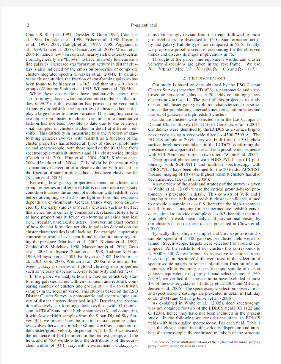
2.THE EDISCS DATASET
Our study is based on data obtained by the ESO Distant Cluster Survey(hereafter,EDisCS),a photometric and spec-troscopic survey of galaxies in20?elds containing galaxy clusters at z=0.4?1.The goal of this project is to study cluster and cluster galaxy evolution,characterizing the struc-ture,stellar populations,internal kinematics,luminosities and masses of galaxies in high redshift clusters.
Candidate clusters were selected from the Las Campanas Distant Cluster Survey(LCDCS)of Gonzalez et al.(2001). Candidates were identi?ed by the LCDCS as a surface bright-ness excess using a very wide?lter(~4500-7500?).The EDisCS sample of20clusters was built from the30highest surface brightness candidates in the LCDCS,con?rming the presence of an apparent cluster and of a possible red sequence with VLT20min exposures in two?lters(White et al.2005). Deep optical photometry with FORS2/VLT,near-IR pho-tometry with SOFI/NTT and multislit spectroscopy with FORS2/VLT have been obtained for the20?elds.ACS/HST mosaic imaging of10of the highest redshift clusters has also been acquired(Desai et al.2006).
An overview of the goals and strategy of the survey is given in White et al.(2005)where the optical ground–based pho-tometry is presented in detail.This consists of V,R and I imaging for the10highest redshift cluster candidates,aimed to provide a sample at z~0.8(hereafter the high-z sample) and B,V and I imaging for10intermediate–redshift candi-dates,aimed to provide a sample at z~0.5(hereafter the mid-z sample).1A weak-shear analysis of gravitational lensing by our clusters based on these data is presented in Clowe et al. (2005).
Typically4hrs–(high-z sample)and2hrs–exposure(mid-z sample)spectra of>100galaxies per cluster?eld were ob-tained.Spectroscopic targets were selected from I-band cat-alogues.At the redshifts of our clusters this corresponds to ~5000±500?rest frame.Conservative rejection criteria based on photometric redshifts were used in the selection of spectroscopic targets to reject a signi?cant fraction of non–members while retaininig a spectroscopic sample of cluster galaxies equivalent to a purely I-band selected one.A pos-teriori,we veri?ed that these criteria have excluded at most 1%of the cluster galaxies(Halliday et al.2004and Milvang-Jensen et al.2006).The spectroscopic selection,observations and spectroscopic catalogs are presented in detail in Halliday et al.(2004)and Milvang-Jensen et al.(2006).
As explained in White et al.(2005),deep spectroscopy was not obtained for two of the EDisCS?elds(Cl1122and Cl1238),hence they have not been included in the present study.In the following we consider the other18EDisCS ?elds with high quality spectroscopy.For each?eld,Table1 lists the cluster name,redshift,velocity dispersion and num-ber of spectroscopically con?rmed members of the structure 1In practice,the redshift distributions of the high-z and the mid-z samples partly overlap,as can be seen in Table1.
Star forming galaxies3 TABLE1
ED IS CS CLUSTERS.
Cluster Cluster zσ±δσN mem N[Oii]Imaging R200f[Oii]f uncorr
[Oii]f lens
[Oii]
f1Mpc
[Oii]
(Mpc)
N OTE.—Col.(1):Cluster name.Col.(2):Short cluster name.Col.(3)Cluster redshift.Col.(4)Cluster velocity dispersion.Redshifts and velocity dispersions are taken from Halliday et al.(2004)and Milvang-Jensen et al.(2006).Col.(5)Number of spectroscopically con?rmed members.Col.(6)Number of members used for computing the[O II]fraction of Col.(9).Col.(7)Available imaging.A+sign indicates those clusters with HST imaging.Col.(8)R200in Mpc.Col.(9)[O II]fraction within R200corrected for completeness.Col.(10)[O II]fraction within R200uncorrected for completeness.Col.(11)[O II]fraction computed within a radius R200derived from the lensing estimate ofσ(Clowe et al.2005).An asterisk indicates systems with additional mass structures along the line of sight,whose lensingσis probably overestimated.Col.(12)[O II]fraction computed within a radius=1Mpc.
that was targeted for spectroscopy and that forms the basis of our study.
3.DERIVING THE[OII]FRACTIONS IN CLUSTERS AT HIGH
REDSHIFT
In this paper we wish to investigate the incidence of ac-tively star–forming galaxies as a function of cluster velocity dispersion,and how this evolves with redshift.We do this by analyzing the proportion of galaxies with a signi?cant[O II] emission line at3727?,a reliable signal of ongoing star for-mation.Dust and metallicity variations affect signi?cantly the strength of the[O II]line,and a quantitative estimate of the star formation rate from the line?ux depends on slit coverage of the galaxy area and spectral extraction method.However, when the limit for line detection is suf?ciently low,the simple presence or absence of this line in emission provides a clean estimate of the incidence of star-forming galaxies in different environments and at different redshifts.2
EDisCS spectra have a dispersion of 1.32?/pixel and 1.66?/pixel depending on the observing run,with a FWHM resolution of~6?,corresponding to rest frame3.3?at z=0.8 and4.3?at z=0.4.The equivalent widths of[O II]were mea-sured on the spectra with a line-?tting technique that follows the one used by the MORPHS collaboration as in Dressler et al.(1999).With this method each1D spectrum is inspected interactively.Each2D spectrum was also inspected to con-?rm the presence of an eventual line in1D:this is especially useful to assess the reality of weak[O II]lines.
2If an AGN is present,this can contribute to the emission line?ux.How-ever,in the great majority of cases an AGN with an emission line spectrum is associated with some level of star formation activity(e.g.Heckman et al. 1995,Cid Fernandes et al.2004and references therein),therefore the con-tamination of the population of[O II]emitters from passive galaxies is bound to be negligible.
We classify as star–forming galaxies those with an equiva-lent width(EW)of[O II]and
For each EDisCS cluster,we have computed the fraction of star–forming cluster members as the fraction of spectroscop-ically con?rmed members3with a rest frame EW([O II])≤?3?.Errorbars on the fractions have been computed using Pois-sonian statistics.We consider only galaxies located within the projected radius delimiting a sphere with interior mean den-sity200times the critical density(R200)and with an absolute V magnitude brighter than M V lim.M V lim was varied with red-shift between-20.5at z=0.8and-20.1at z=0.4to account for passive evolution.Our spectroscopy would allow an anal-ysis for galaxies up to0.5mag fainter than these limits,but for this study M V lim was chosen to carry out a comparison with the Sloan dataset(see below).Rest frame absolute mag-nitudes were estimated for each EDisCS galaxy as in Rudnick et al.(2003)and are given in Rudnick et al.(2006).R200was computed from the cluster velocity dispersionσas in Finn et al.(2005):
R200=1.73
σ
4
Poggianti et al.
01000
200005001000150020002500
01000
20000500100015002000
250001000
2000
0500100015002000250001000
200005001000150020002500
01000
20000500100015002000
250001000
2000
0500100015002000250001000
20000
5001000150020002500X
01000
20000
5001000150020002500X
01000
2000
5001000150020002500X
F I
G .1.—XY pixel positions of objects with spectra in the EDisCs mid-z ?elds.Filled dots represent spectroscopically con?rmed cluster members.The circle with radius R 200,centered on the BCG,is shown.The axis units are pixels =0.2′′.
The cluster center was assumed to coincide with the Bright-est Cluster Galaxy (BCG),that was identi?ed interactively on the EDisCS VLT images.A list of the BCGs can be found in White et al.(2005).For most of the clusters,our spectroscopy samples at least out to the cluster R 200or beyond (Figs.1and 2).A few clusters have incomplete radial sampling due to their large projected radii (most notably,Cl 1232,Cl 1411and Cl 1138),or to the BCG location close to the FORS2?eld edge (Cl 1227):when relevant,these cases will be commented separately.
The fractions of [O II ]emitters were computed weighting each galaxy for incompleteness of the spectroscopic catalog,taking into account the completeness as a function of galaxy magnitude and position,as described in Appendix A.Ignor-ing these weights,however,does not affect signi?cantly our results,as discussed in §5.In Appendix B,we show that the color distributions of the ?nal spectroscopic sample and its parent photometric sample are indistinguishable according to a KS test,and therefore no color bias is present in the spec-troscopic sample we are using.
The exposure times of the EDisCS spectroscopy (4hrs and 2hrs of VLT for the high-and mid-z samples,respectively)were chosen to allow not only a redshift determination,but also a detailed spectroscopic analysis of emission and absorp-tion features.As a consequence,the fraction of spectroscopic targets for which no redshift could be derived is negligible:only 3%of the spectra brighter than the magnitude limit used here did not yield a redshift.4Hence,no correction is required to account for the success rate (percentage of spectra provid-ing a redshift)as a function of magnitude or color.
The [O II ]fractions derived as described above are given in column 9of Table 1.For comparison,the table also lists the [O II ]fractions computed without applying completeness cor-rections (column 10),or with different radial criteria:within R 200as derived from the σbased on the weak lensing analysis of Clowe et al.(2005)(column 11)and within a ?xed metric
4
As discussed in Halliday et al.(2004),the spectra show that most of these are bright lower redshift galaxies (non-members of our clusters)observed in a red rest-frame spectral region that is featureless and thus makes it hard to derive a secure redshift.
Star forming galaxies
5
01000
200005001000150020002500
01000
200005001000150020002500
01000
2000
0500100015002000250001000
200005001000150020002500
01000
200005001000150020002500
01000
2000
0500100015002000250001000
20000
5001000150020002500X
01000
20000
5001000150020002500X
01000
2000
5001000150020002500X
F I
G .2.—Same as Fig.1but for the high-z EDisCS ?elds.
radius equal to 1Mpc (column 12).For all structures except one (Cl 1420),the different estimates of the [O II ]fraction are compatible within the errors.
3.1.Other high-z cluster samples
The EDisCS dataset is homogeneous for cluster and galaxy selection and data quality,thus an internal comparison among clusters is straightforward.A comparison with other spec-troscopic surveys of distant clusters requires much more cau-tion,as a number of conditions need to be met:such a survey should cover out to R 200and be representative of a magnitude-limited sample of galaxies selected in the rest-frame at 4500-5500?.A reliable determination of the cluster velocity dis-persion should be available,as well as accurate EW([O II ])measurements highly complete down to 3?for galaxies down to the absolute magnitude limit M V lim .These are de-manding requirements that are largely ful?lled by surveys of just a few distant clusters in the literature.
The list of additional distant clusters we include in our anal-ysis is given in Table 2.Seven of these clusters are taken from
the MORPHS survey (Dressler et al.1999,Poggianti et al.1999,hereafter D99and P99)and are at redshifts covering the low redshift end of the EDisCS redshift range (z =0.38?0.55).Two other clusters are MS1054-03at z=0.83taken from van Dokkum et al.(2000)(hereafter vD00),and Cl1324+3011at z=0.76from Postman et al.(2001)(hereafter POL01).
Measurements of the EW([O II ])were taken from these au-thors,assuming their spectroscopic catalogs are highly com-plete for EW([O II ])
6Poggianti et al.
TABLE2
O THER DISTANT CLUSTERS.
Cluster zσ±δσN[Oii]Imaging R200(Mpc)FOV f[Oii]Ref1a Ref2b
N OTE.—Col.(1)Cluster name.Col.(2)Cluster redshift.Col.(3)Cluster velocity dispersion.Col.(4)Number of galaxies members of the cluster used for the calculation of the[O II]fraction.Col.(5)Photometric band used for selection of spectroscopic targets and magnitude limit we adopted to be compatible with EDisCS.Col.(6)R200in Mpc.Col.(7)Field-of-view of the spectroscopic coverage.Col.(8)[O II]fraction.Col.(9)-(10)References.An additional cluster presented in POL01has later been shown to be composed of4distinct clusters for which a spectroscopic catalog should become available in the future(Gal& Lubin2004).A cluster from Postman et al.(1998)was not included because its completeness function was not available.The cluster and the group at z=0.59 in the MS2053?eld of Tran et al.(2005)haveσ=865and f[Oii]=0.34,andσ=282and f[Oii]=0.67,respectively,where f[Oii]is given by the authors for galaxies with EW([O II])
a Source for the[O II]measurements and completeness functions.
D99=Dressler et al.1999;P99=Poggianti et al.1999;vD00=van Dokkum
et al.2000;PLO01=Postman,Lubin&Oke2001.
b Source for the cluster velocity dispersion.GM01=Girardi&Mezzetti
2001;LOP02=Lubin,Oke&Postman2002.
while the EDisCS and all other clusters used in this analy-sis were selected at~5000±500?rest frame.Though the estimate of the[O II]fraction in clusters in these external sam-ples cannot be carried out in a way that is fully homogeneous with the analysis performed on the EDisCS data,due to the slight differences in radial coverage,magnitude limit and so on,such differences are suf?ciently small to allow an interest-ing comparison with the EDisCS data:this will be presented in§5.
4.THE[OII]FRACTIONS AT LOW REDSHIFT:SLOAN
In order to compare with clusters at low redshift,we con-structed a local comparison sample from the spectroscopic Sloan Digital Sky Survey.Rather than trying to obtain a sam-ple with the largest possible number of clusters,we aimed to build a sample with selection criteria similar to EDisCS.For simplicity,we used the Abell cluster catalog.Its selection is based on(projected)overdensities of galaxies,which can be regarded as being similar to the selection of EDisCS clusters, that were chosen by their light excess over the background. Our Abell sample was built according to the following steps:
1)At the time of sample selection,the most comprehensive compilation of properties of Abell clusters was by Struble& Rood(1991).From this,we selected clusters with a redshift estimate based on at least two galaxies.This yields774clus-ters.
2)Only clusters with0.04
3)For each cluster,we identify galaxies from the spectro-scopic DR2SDSS catalog which lie within one Abell radius (R A=1.7′/z)from the cluster center quoted by Struble& Rood(1991).Only clusters with at least20matched galax-ies are retained(32clusters).
4)At this stage,the image of each cluster was inspected interactively.We restricted the sample to clusters that are well separated from the survey boundaries,and we identi?ed a BCG from the SDSS imaging data.Redshift histograms were also inspected to verify the presence of a concentration of galaxies at the redshift given by Struble&Rood(1991). These constraints yield a sample of24clusters,to which we add two clusters with redshifts slightly lower than0.04and two with redshifts slightly higher than0.085.The?nal list of 28clusters is presented in Table3.
5)As for the EDisCS sample,we rely on the biweight esti-mator of Beers et al.(1990)for determining the cluster red-shift and velocity dispersion,as described in Appendix C. Once our low–redshift comparison sample was selected,a number of steps were taken to ensure a meaningful compari-son with our high-z sample.
1)The Sloan spectroscopic target selection was performed in the r band(r<17.7).In order to more closely approximate the rest-frame EDisCS selection wavelength,we extracted a g-selected sample from the Sloan spectroscopic catalogs.This corresponds to the subset of galaxies with g≤18:brighter than this limit,99%of the galaxies have r<17.7and their g-magnitude distribution follows closely the distribution in the whole g-band photometric sample.Galaxies brighter than g=12and r=12were excluded,being brighter than any clus-ter member of the clusters considered.Therefore,the Sloan
Star forming galaxies
7
-10
-20
-30
-10
-20
-30
our EW([OII]) measurement
F I
G .3.—EW([O II ])s of Sloan spectra in plate #973.The measurement
obtained with the Ediscs method is compared with the EW listed by Sloan.The inset is a blow-up of the lower left corner of the plot,in which errorbars are omitted for clarity.In this plot,EDisCS EWs =0correspond to those spectra in which the line is not detected and the spectral ?uctuations in that region are considered noise.Since the Sloan measurements are fully auto-matic,these cases can yield a non-null negative or positive EW value,that is however consistent with zero within the errorbar in most cases.
spectroscopic sample we used is the subset of the Sloan cata-logs with 12 2)Each galaxy in the spectroscopic catalog was assigned completeness weights as a function of magnitude and posi-tion comparing,cluster by cluster,the number of galaxies in the Sloan spectroscopic and photometric (g -band)catalogs,as done for EDisCS (see Appendix A).As in EDisCS,essentially all targeted galaxies (99.9%)yield a reliable redshift (Strauss et al.2002),thus no correction is required to account for the spectroscopic success rate. 3)The analysis of the fraction of [O II ]-emitters was car-ried out on the Sloan data as for EDisCS.The center of each cluster was assumed to coincide with the BCG.Only galaxies within R 200were considered,down to an absolute V magnitude limit =?19.8,corresponding to the limit at which spectroscopic incompleteness sets in at these redshifts in the Sloan sample.This limit was used to determine the absolute magnitude limit in the distant clusters,once pas-sive evolution was taken into account.Galaxy absolute V magnitudes were obtained from the absolute Petrosian magni-tudes in the Sloan system using the transformation of Blanton (https://www.doczj.com/doc/f98161388.html,/?mb144/kcorrect/linear.ps). 4)The star-forming fraction was computed as the frac-tion of galaxies with EW([O II ]) TABLE 3S LOAN CLUSTERS . Cluster z σ±δσ N [Oii ]R 200 f [Oii ] f uncorr [Oii ] N OTE .—Col.(1):Cluster name.Col.(2)Cluster redshift.Col.(3)Cluster velocity dispersion.Col.(4)Number of members used for computing the [O II ]fraction.Col.(5)R 200in Mpc.Col.(6)[O II ]fraction corrected for completeness.Col.(7)[O II ]fraction uncorrected for completeness. son of the fraction of galaxies with EW([O II ])and To test our results on a larger control sample that,how-ever,resembles less closely the EDisCS sample for selection and characteristics,we also chose a second cluster sample in the SDSS from the C4catalog of Miller et al.(2005)at redshift 0.04≤z ≤0.08.The purity of the C4sample is discussed in Miller et al.(2005).Such a sample is more 5 As visible in the inset of Fig.3,only 2cases of small discrepancy are found among the 162galaxies:galaxy #506with EW(Sloan)=-2.6±0.6and EW(EDisCS)=-3.4±0.5?,and galaxy #369with EW(Sloan)=-3.5±1.1and EW(EDisCS)=0,because no line appears to be present from a visual inspec-tion of the spectrum. 8Poggianti et al. prone to be contaminated by?laments,sheets and multiple structures yielding an overestimatedσ.To minimize the con-tamination of structures with severely overestimated velocity dispersion,we retained only clusters withσ≤1500kms?1, σ≤σC4+200kms?1and a number of galaxies within3σfrom the cluster redshift and within R200equal or greater than7, whereσwas measured from the Sloan spectroscopic tables as described in Appendix C andσC4is the velocity dispersion given by Miller et al.(2005).Clusters with clear multiple peaks in the redshift histograms indicating that theσis unre- liable were excluded. Since all but one of the EDisCS structures have at least8 members within these magnitude and radial limits(N[Oii]in Table1),we included only C4clusters with at least8members usable to compute the[O II]fraction.Our?nal C4-based sam- ple consists of88clusters,whose centers were taken to coin- cide with the BCG listed by Miller et al.(2005).6The[O II] fraction of these clusters was computed from a g-selected sample of galaxies within R200and with M V was done for the Abell sample.For the C4-based sample we did not apply completeness weights,given that these cor- rections did not affect signi?cantly the[O II]fractions of the Abell clusters(see Table3). 5.RESULTS 5.1.Star formation activity at high redshifts as a function of the cluster mass Our main result is shown in Fig.4.The left panel presents the fraction of[O II]emitters as a function of cluster velocity dispersion for EDisCS clusters(?lled small circles),and for the other clusters at z=0.4to0.8whose data were taken from the literature as described in Sec.3.1. Most datapoints occupy a stripe in this diagram,indicating that most clusters follow a broad anticorrelation between the fraction of star-forming galaxies and the cluster velocity dis-persion:generally,more massive clusters have a lower frac- tion of star-forming galaxies.When including all clusters,a Kendall test shows that an anticorrelation between cluster ve- locity dispersion and star-forming fraction is present with a 97.1%probability.There are evident outliers that do not fol- low the[O II]-σtrend de?ned by the majority of clusters.The most evident outliers are Cl1119and Cl1420,two groups withσ<400kms?1that will be discussed further in§5.5.The Kendall probability becomes99.9%when excluding these two outliers.The probabilities excluding non-EDisCS data- points become48.0%and96.2%when the two outliers are included and excluded,respectively. Assuming that the cluster velocity dispersion is related to the mass of the system7,the[O II]-σrelation shown in the left panel of Fig.4suggests that it is the mass of the system, though with a signi?cant scatter,that largely determines what proportion of its member galaxies are forming stars at z~0.6. 6The BCG was chosen by Miller et al.to be the brightest entry in the SDSS catalog within500h?1kpc from the peak of the C4density?eld,with EW(Hα)>?4?and within4σfrom the cluster redshift,or with no spec- troscopy but brighter than m r=19.6and M r=?19.8with colors lying within the cluster color-magnitude sequence and no more than two magnitudes dim- mer than the BCG identi?ed based on the4σcriterion. 7We note that two EDisCs clusters,Cl1216and Cl1232,show evidence for substructure and therefore in principle their velocity dispersions may be a poor indicator of their masses(Halliday et al.2004).However,a subse- quent weak lensing analysis of EDisCS clusters has showed that substruc- ture does not strongly affect the spectroscopic measurement of their veloc- ity dispersion,con?rming within the errors the spectroscopic estimate ofσ (σ=1152+70 ?78for Cl1216,andσ=948+50 ?55 for Cl1232,Clowe et al.2005). Given the scatter and the outliers in this plot,however,it is uncertain whether this is better described as a broad relation between the[O II]fraction andσ,or as an upper envelope.In fact,the most notable feature of this diagram is the absence of datapoints in the upper right corner,above the most popu- lated stripe.This envelope in the[O II]fraction versusσplane seems to imply that at z=0.4?0.8a system of a given mass can have at most a certain fraction of star-forming galaxies or,equivalently,must have at least a given fraction of galax- ies that are already passive at this epoch.More massive sys- tems have a lower maximum-allowed fraction of star-forming galaxies or,equivalently,a higher minimum-allowed fraction of passive galaxies. The solid line in Fig.4is a"hand-drawn"description of this upper envelope8: f[Oii]=?0.74×( σ Star forming galaxies 9 0500 1000 0.20.40.60.81 Cluster velocity dispersion 0500 1000 0.2 0.4 0.6 0.8 1 Cluster velocity dispersion F I G .4.—Left.The [O II ]-σrelation in clusters at 0.4≤z ≤0.8.The fraction of cluster members within R 200with [O II ]emission is plotted versus the cluster velocity dispersion.Solid black dots represent EDisCS datapoints in each one of the 18?elds,as in Table 1.The red crosses are for MORPHS clusters;the red solid large circle is the cluster MS1054-03from van Dokkum et al.and the red empty circle is Cl1324+3011from Postman et al.Errorbars on the fractions are Poissonian.The solid line across the plot is taken as a description of the upper envelope of the high-z points (see text).The same line is repeated in the right panel,to illustrate the differences.At high-z,the majority of systems group around this line,while at low-z (right panel)the great majority fall well below the line.Right.The [O II ]-σrelation in low redshift clusters from Sloan described in §4.Empty circles indicate those Sloan clusters slightly outside of the preferred redshift range.The two dotted lines represent the eye-?tted most heavily populated region in the plot. are shown in Fig.6.These clusters con?rm the main trends observed in the Abell sample:for σ>550kms ?1,the [O II ]fraction does not seem to depend on σand is smaller than 0.3for the great majority of clusters.At σ≤500kms ?1,many systems have an f [Oii ]higher than 0.3,though there are also systems with low σand low f [Oii ].While from the Abell sam-ple there appears to be a trend of increasing average [O II ]fraction towards lower velocity dispersions,for the C4clus-ters it is unclear whether there is a trend at σ<500kms ?1,or simply a large scatter in the [O II ]fraction at low σ.We note that the trend of rising average f [Oii ]observed in the Abell sample is in excellent agreement with the results of Martinez et al.(2002)who found the average fraction of emission-line galaxies to decrease monotonically with virial mass for groups (1012?2×10¹⁴M ⊙)from the 2dF Galaxy Redshift Survey.The result from Martinez et al.(2002)parallels the trend of increasing early-type fractions towards higher ve-locity dispersion in the poor groups studied by Zabludoff &Mulchaey (1998),who noted that the early-type fractions in the most massive groups of their sample were comparable to those found in rich clusters.A rising fraction of “late-type galaxies”(de?ned on the basis of their color and star forma-tion from emission lines)towards lower velocity dispersions is also found below 500kms ?1in Sloan groups by Weinmann et al.(2006).Our low-z trends also agree with the fraction of passive galaxies in 2dF groups from Wilman et al.(2005b,see their Fig.7).9Keeping in mind the caveat of a larger scat-9 For clusters,Biviano et al.(1997)also found a trend with σin the fraction ter in the C4sample at low σ,in the following we will adopt as reference the rising trend observed in the Abell sample.As we will see,this does not in?uence our main conclusions.In fact,the most relevant and striking aspect of the Abell and C4comparison is that both samples show a break in the behaviour of the [O II ]fraction with σat the same velocity dispersion (~500kms ?1)and that most clusters above this σhave a fraction of star-forming galaxies around 20%.As we will discuss later,this critical threshold in σis an important observational landmark for inferring the effects of the envi-ronment on galaxy star formation histories.10 A schematic view of the evolution in the [O II ]–σdiagram is presented in Fig.7.The solid line and the two dotted lines illustrate the position of the most densely populated regions at high and low redshift,respectively,reproducing the average observed trends followed by most clusters in the two panels of Fig.4. The arrows in Fig.7indicate the average velocity dispersion of z =0.6progenitors of systems of different masses at z =0. of emission-line galaxies in the ESO Nearby Abell Cluster Survey between 400and 1100km s ?1.A direct comparison with our results cannot be carried out,due to the very different threshold of line strength adopted for identifying emission-line galaxies,but they found that on average the mean emission-line fraction in three bins of σdecreased towards higher σ.If we analyzed the [O II ]fraction for our Sloan clusters in three similarly wide bins of σ,instead of presenting the results cluster by cluster,we would obtain a similar trend.10We note that our low-z samples are composed for the great majority of structures with σbetween 350and 900km s ?1,therefore they do not allow an exploration of the properties of the most massive and the least massive systems. 10 Poggianti et al. 0.4 0.50.60.70.8 -1-0.5 0.5 1 Redshift F I G .5.—Residuals of the [O II ]fraction of EDisCS clusters with respect to the line drawn in the [O II ]-σrelation at high-z shown in Fig.4,plotted versus cluster redshift.The solid line is the least squares ?t having excluded the two outliers (Cl 1119and Cl 1420),which are the two points with residuals 0500 1000 0.2 0.4 0.6 0.8 1 Cluster velocity dispersion F I G .6.—The [O II ]-σrelation in Sloan clusters at 0.04 0500 1000 0.2 0.4 0.6 0.8 1 Cluster velocity dispersion F I G .7.—Evolution of the [O II ]-σrelation inferred from observations at different redshifts.The solid line and the two dotted lines represent the observed relations followed by the majority of clusters at high-and low-z,respectively.These are the same lines shown in the left and right panels of Fig.4.The arrows identify the average progenitors at z =0.6of clusters of different mass at z =0as expected from simulations,considering the fact that the cluster mass,hence its velocity dispersion,evolves too (see text for details).If σdid not evolve with time,the arrows would be vertical in this plot. This was computed from the assembly history given by high–resolution N-body simulations by Wechsler et al.(2002),adopting concentration parameters as in Bullock et al.(2001)and computing the relation between mass of the system and σas in Finn et al.(2005):M sys =1.2×10¹⁵( σ Star forming galaxies 11 0500 10001500 500 1000 1500 Velocity dispersion (z=0) F I G .8.—Relation between the velocity dispersion of systems at z =0and at z=0.76.Empty triangles are average values derived analytically from Wechsler et al.(2002)and eqn.4,as described in §5.2.Filled circles are results for 90haloes from the Millennium Run simulation (Springel et al.2005),as described in §5.2. of the velocity dispersions estimated from the two indepen-dent simulations.In the following,we use the average evo-lution of σderived from Wechsler et al.(2002)and eqn.(4)to establish the evolutionary link between low-z and high-z structures.11In Table 4,we list the average f [Oii ]fractions ob-served at high–and low–redshift as a function of the cluster velocity dispersion and mass at z =0,the corresponding aver-age σand mass of that structure at z =0.6,and the difference ?f in f [Oii ]between the two redshifts.12 Fig.7and Table 4show that the strongest evolution in mass and in velocity dispersion is expected for the most massive structures.The same ?gure and table also illustrate that the observed change in star–forming fraction between z =0.6and z =0is maximum instead for intermediate-mass structures ,those with σ~5?600kms ?1at z =0and ~450?500kms ?1at z =0.6.The evolution is smaller at both higher and lower masses,but is still signi?cant even for the most massive sys-tems in the Sloan sample.13In the mass range we observe, 11 We note that this is done selecting haloes at z =0and computing the av-erage projected velocity dispersion of their “main progenitor”at z =0.6.We have veri?ed that selecting haloes at z =0.6and following their descendants to z =0gives similar results,albeit the amount of evolution in σturns out to be slightly smaller in this case.The differences found with the two selection methods increase with the halo velocity dispersion ranging from less than 10km s ?1for systems up to 500km s ?1to about 100km s ?1for systems with 1000km s ?1. 12We stress that Table 4extends to lower and higher masses than those probed by our sample at low redshift.Therefore,for systems with σbelow 350and above 1000km s ?1at z =0the values listed are extrapolations of the observed trends,not con?rmed by any observational evidence.According to these extrapolations,no change in [O II ]fraction with redshift would be ob-served for systems below 200km s ?1.At these low masses also the evolution of σ(mass)is negligible (Table 4). 13It is worth noting that the star-forming fractions in clusters with σ>1000km s ?1on average are quite similar at z =0.6and z =0(compare the TABLE 4 M EAN EVOLUTION BETWEEN Z =0AND Z =0.6OF THE VELOCITY DISPERSION σ,THE MASS OF THE SYSTEM M sys AND THE [O II ] FRACTION .σz =0M sys z =0f [Oii ]z =0σz =0.6 M sys z =0.6f [Oii ]z =0.6?f km s ?1 M ⊙/h km s ?1 M ⊙/h N OTE .—Col.(1)Velocity dispersion of a system at z=0.Col.(2)Corre-sponding mass of the system at z=0in units of solar masses/h .The relation between σz =0and the mass is computed according to eqn.(4).Col.(3)Aver-age [O II ]fraction at z=0for a system of σz =0,derived from eqn.(3).Col.(4)Mean velocity dispersion at z=0.6of a system with σz =0as in col.1.σz =0.6is computed from Col.5according to eqn.(4).Col.(5)Mean mass at z=0.6of a system with M z =0as in col.2.The relation between mean mass at z=0and mean mass at z=0.6is computed according to Wechsler et al.(2002)(see §5.2).Col.(6)Average [O II ]fraction at z=0.6for a system of σz =0.6as in col.4,derived from eqn.(2).Col.(7)Difference between the [O II ]fractions at z=0.6and z=0(col.6-col.3). the change in the average star–forming fraction ?f ranges between 20-30%and 50%. It is essential to keep in mind that the trends in Fig.7and Table 4depict an average evolution apparently followed by the majority of systems,but a large scatter is present in the observed [O II ]-σrelation at all redshifts,and the evolution of the cluster masses is expected to proceed with a signi?cant scatter too,as shown in Fig.8. In this section we have shown that the fraction of star–forming (and,conversely,passive)galaxies in clusters has evolved signi?cantly between z ~0.6and z =0.For the ?rst time,we can quantify how the average evolution varies with the mass of the system.Why the proportion of passive/star–forming galaxies broadly correlates/anticorrelates with the ve-locity dispersion of the system for most clusters at high-z,why this proportion evolves with redshift,why the evolution is maximum for intermediate-mass systems and why there is no clear trend with σat z=0for systems more massive than ~550kms ?1are questions that will be addressed in §6. 5.3.Other environments at high-z About 35%of the galaxies in the EDisCS spectroscopic cat-alog reside in the 18structures that have been discussed so far.The other spectra can be used to investigate other envi-ronments at high redshift,such as groups and the “?eld”.We have identi?ed other structures in our spectroscopic sample as associations in redshift space.Given our selection left panel in Fig.4with the right panel in the same ?gure and with Fig.6).However,as shown in Fig.7and Table 4,clusters with σ>1000km s ?1at z =0are those whose mass evolved the most between the two redshifts.Their progenitors at z =0.6were ~800km s ?1systems,whose star-forming fraction was higher than that of their descendants at z =0.Thus,also the most massive systems at z =0on average have experienced a signi?cant evolution of their fraction of star-forming galaxies. 12 Poggianti et al. TABLE 5 O THER ED IS CS STRUCTURES . Cluster z σ±δσN mem N [Oii ] f [Oii ] Dist /σ N OTE .—Col.(1)Name of the structure.Col.(2)Redshift.Col.(3)Ve-locity dispersion.Col.(4)Number of spectroscopically con?rmed members.Col.(5)Number of galaxies members of the cluster used for the calculation of the [O II ]fraction,hence brighter than the adopted magnitude limit.Col.(6)[O II ]fraction.Col.(7)Distance from another structure in units of σof the most massive of the two. a named Cl 1103.7-1245a in White et al.(2005). 00.20.4 0.60.81 10 20 30 40 50 z 00.20.4 0.60.81 2 4 6 8 10 12 z F I G .9.—Left.Redshift distribution of our ?eld spectroscopic sample.Right.Redshift distribution of galaxies in our poor groups. criteria for spectroscopic targets (§2and Halliday et al.2004),we can treat the spectroscopic catalog in a redshift slice close to the redshift targeted in each ?eld as a purely I-band se-lected sample (Milvang-Jensen et al.2006).To ensure that no selection bias can be present,we choose conservative redshift limits and we only consider galaxies within ±0.1in z from the cluster targeted in each ?eld.With these criteria we can study two other clusters (σ>400kms ?1),listed in Table 5,and several groups (σ<400kms ?1). Two types of groups have been isolated.Six structures have at least 7member galaxies with spectroscopic redshifts.For these,velocity dispersions have been computed.In the fol-lowing we will refer to these as “groups”.These are listed in Table 5and are among the groups studied in detail in Halliday et al.(2006). Associations in redshift space with between 3and 6galax-ies in our spectroscopic catalog have been treated separately,and hereafter will be referred to as “poor groups”.In total our poor groups comprise 84galaxies,whose redshift distri-bution is shown in Fig.9.We did not attempt to derive veloc-ity dispersions for these systems given the small number of redshifts. Any other galaxy in our spectroscopic catalog that was not 05001000 0.2 0.4 0.6 0.8 1 Cluster velocity dispersion F I G .10.—Same as Fig.4,but now including also other environments.Empty triangles are other EDisCS structures with at least 7spectroscopically con?rmed members as in Table 5.The average [O II ]fraction and correspond-ing errorbars in poor groups (those between 3and 6spectroscopic members)are shown with green dashed lines.The [O II ]fraction among ?eld galaxies (see text)and its errorbars are shown as blue solid lines. a member of any of our clusters,groups or poor group as-sociations,will be hereafter named a “?eld”galaxy.Our ?eld sample is composed of 162galaxies,whose redshift distribution is shown in Fig.9.Our “?eld”sample should be dominated by galaxies in regions less populated than the clusters/groups/poor groups we isolated,but will also contain galaxies belonging to structures that were not detected in our spectroscopic catalog. The [O II ]fractions in these additional structures and in the ?eld have been computed for galaxies with absolute magni-tudes brighter than the limit adopted for the main 18structures described in §3.No radial distance criterion has been intro-duced for the additional structures (those presented in Table 5and the poor groups)and the ?eld.The lack of a radial crite-rion,however,does not signi?cantly affect the [O II ]fractions derived for these systems. The fraction of [O II ]emitters we ?nd in the “?eld”is f [Oii ]=0.74and is shown in Fig.10as a solid blue horizontal line with its errorbars.The [O II ]fraction in poor groups is even higher (87%,green dashed horizontal line in Fig.10),though still compatible with the fraction in the ?eld within the errors.The other structures for which we derived a velocity disper-sion are shown in Fig.10as empty triangles.Among these,there are 4systems with very high [O II ]fractions ranging be-tween 83and 100%.In redshift space,these systems are all far from any known cluster,always at least 17σclu away (see Table 5).The other 4additional structures in Fig.10have rel-atively low [O II ]fractions,around 40-50%.Two of these are quite close to other massive structures (7σclu from the most massive cluster in that ?eld,see Table 5). To summarize,both the ?eld and the poor groups contain a high proportion of star-forming galaxies (70to 100%),com- Star forming galaxies13 parable to that observed in more than half of the systems with σ<400kms?1,and in agreement with the line that traces the relation between f[Oii]andσup to the most massive systems. In addition,there are5other groups withσ<400kms?1(in-cluding Cl1119and Cl1420,previously discussed)that have [O II]fractions signi?cantly lower than the rest of the groups and the?eld.Their[O II]fractions are≤50%.We will come back to discussing these systems and describe their properties and those of their galaxy populations in§5.5. 5.4.EW([O II])distributions As shown above,the fraction of star-forming galaxies in high-redshift clusters depends on cluster velocity dispersion. It is interesting to investigate whether also the star formation activity in star-forming galaxies depends onσand,more gen-erally,on environment.In this section we analyze how the distributions of EW([O II])for star–forming EDisCS galaxies vary in the different environments.We do not attempt any comparison with the low-redshift sample,given that a quanti-tative comparison of the EW strength is affected by the uncer-tainties related to aperture effects between z=0.8and z=0. We consider the“environments”de?ned in§5.3,namely clusters,groups,poor groups and?eld.Clusters have been further subdivided into more and less massive clusters.We de?ne as“massive clusters”all clusters in Table1withσ> 800kms?1(Cl1216,Cl1232),and as“less massive clus-ters”those with400<σ<800kms?1(Cl1138,Cl1411, Cl1301,Cl1354,Cl1353,Cl1054-11,Cl1227,Cl1202, Cl1059,Cl1054-12,Cl1018,Cl1040).Among the groups, we consider separately groups with high and low[O II]frac-tions as discussed in the previous section.“Groups with low-emission”are those groups withσ<400kms?1and [O II]fractions signi?cantly below the line in Fig.4(Cl1420, Cl1119,G1_105412,G1_1301,G1_1103).“Groups with high-emission”are those groups withσ<400kms?1and [O II]fractions that roughly follow the line in Fig.4(Cl1037, Cl1103,G1_1040,G2_1040,G1_1054-11).The same radial, magnitude and EW limits and completeness weights used for computing the[O II]fractions have been applied to the EW distributions. We have studied the proportion of star–forming galaxies with strong(EW 15The presence of some galaxies with very high EWs in massive clusters is consistent with the detection of some spirals with enhanced star formation in rich clusters(see https://www.doczj.com/doc/f98161388.html,vang-Jensen et al.2003,Bamford et al.2005and references therein). F IG.11.—Fraction of star–forming galaxies with a strong,moderate and relatively weak equivalent width of[O II]in different environments.Environ-ments are located on the x-axis in order of increasing average[O II]fraction as from Fig.4.The fraction of galaxies with relatively low EW(?20 weighted and unweighted distributions(solid and empty sym-bols in Fig.11),except for the fraction of galaxies with strong EWs in the?eld which is signi?cantly reduced when the com-pleteness correction is ignored.The minimum errorbar for each point in Fig.11is computed from Poissonian statistics, while total errorbars have been increased to take into account the difference between weighted and unweighted values.To-tal errorbars are plotted in Fig.11. Thus,it is not only the proportion of galaxies with active star formation that changes as a function of environment,but also the star formation properties in star-forming galaxies. The two things are closely related to each other,following a parallel progressive trend:the distribution of EW([O II]) is more skewed towards high values for environments with higher[O II]fractions.This seems to be at odds with the uniformity of the EW(Hα)distribution as a function of en-vironment found by Balogh et al.(2004)for local samples, although a study analogous to ours has not been carried out at low-z. In principle,a different EW distribution could simply re?ect a different luminosity distribution of galaxies in the different environments,since lower luminosity star–forming galaxies are known to have on average higher EWs than bright star–forming galaxies.To investigate whether the differences in the EW([O II])distributions are due to a different luminos- 14Poggianti et al. ity distribution with environment,or whether it is the SF in galaxies of similar luminosity that changes with environment, we plot in Fig.12the number density distribution of star–forming galaxies in a two-dimensional space of galaxy abso-lute V magnitude and EW([O II]). Following a well known trend,galaxies occupy a charac-teristic triangular region in this diagram:in all environments, there are no or at most a few bright galaxies with EW([O II] )stronger than?20?,while going to fainter magnitudes the EW distribution extends to stronger and stronger EWs.In fact,fainter galaxies span a wide range of EWs,while the brightest galaxies are con?ned to small/moderate EWs. While these are the general trends,the maps also show some interesting variations with environment.Groups with low[O II]fractions(bottom left panel)lack a signi?cant pop-ulation of faint galaxies with moderate and strong EWs that are present in the other environments.In these groups,star–forming galaxies have weak EWs,regardless of their lumi-nosity.According to a KS test,considering only star-forming galaxies with M V=?20to?21.5,the EW distribution in groups with low[O II]emission is different from the summed distribution in all other environments at the99.9%con?dence level(99.4%if the EW distributions are not weighted for com-pleteness). Inspecting the histograms of EW([O II])(on the right side of each panel),the?eld and poor group environments(mid-dle and right top panels)display an excess of galaxies with intermediate and strong EWs compared to both massive and less massive clusters(middle and right bottom panels).This is the same effect seen in Fig.11,that shows that the frac-tion of galaxies with intermediate+strong EWs increases go-ing from clusters to poor groups and the?eld.The distri-butions of absolute magnitudes of star-forming galaxies are presented in the top histogram of each panel.These show that the magnitude distribution in the?eld and poor groups is skewed towards fainter average magnitudes than in clusters of all masses.In fact,the absolute magnitude distribution in the?eld+poor groups differ from that in clusters at the99.9% con?dence level.In this case,the difference is not signi?-cant if the distributions are unweighted.Moreover,at a given faint luminosity,galaxies in the?eld and poor groups tend to have stronger EWs on average than similarly luminous star-forming galaxies in clusters(see the variation of the Y posi-tion of the red/yellow highest peak at faint magnitudes in the maps of?eld/poor-groups versus clusters).The difference in the EW distribution for faint galaxies(M V=?20to?21.5)in ?eld+poor groups compared to massive+less massive clusters is signi?cant at the99.9%level(96.0%if unweighted). Thus,the behaviour of the EW([O II])distributions with environment seen in Fig.11appears to be the result of a com-bination of different EWs at a given faint luminosity(stronger EWs in environments with higher star-forming fractions)and different luminosity distributions of star-forming galaxies(a higher faint-to-bright galaxy number ratio in environments with higher star-forming fractions). 5.5.Outliers in the[O II]-σrelation It is worth analyzing separately the properties of outliers from the[O II]–σrelation.Here we consider as outliers those EDisCS structures with an[O II]fraction signi?cantly lower than the fractions of the majority of structures of similar ve-locity dispersion. The two most outstanding outliers are two groups,Cl1119 and Cl1420,withσ=165and225kms?1,respectively,and an [O II]fraction<30%.Both of these structures have quite a high number of spectroscopically con?rmed bright mem-bers(>20)within a small velocity dispersion.For Cl1119, the non-detection in the weak lensing analysis and the cor-responding upper limit onσcon?rm the low-mass nature of this system,while for Cl1420a meaningful comparison can-not be performed because the lensing-based estimate is likely contaminated by other mass structures(Clowe et al.2005). Thus,at least for Cl1119this seems to rule out the possibil-ity that the system deviates from the general trend due to its σmeasurement strongly underestimating its mass.Moreover, as shown in column12of Table1,these two systems remain outliers also if we relax the R200criterion and compute the [O II]fraction over a larger?eld.16 Interestingly,besides the low[O II]fractions,these two systems also stand out for their unsually high fraction of early-type galaxies for their velocity dispersion,as found by the analysis of galaxy structural parameters based on2D bulge+disk decomposition(Simard et al.2006),and for their low fractions of blue galaxies(De Lucia et al.2006).The evi-dence for the peculiarity of these outliers is further reinforced by the analysis of the[O II]equivalent width distributions.We have seen in§5.4that the EW distribution in star-forming galaxies of the groups with low[O II]fractions(including Cl1119and C1420)is different from that in any other en-vironment.The population of faint galaxies with strong EWs, common in other environments,is absent in these groups.All of these?ndings(low[O II]and blue fractions,high early-type fractions for their velocity dispersion,as well as pecu-liar equivalent width distribution of[O II])suggest that these groups are intrinsically peculiar when compared to the major-ity of other structures.In fact,the properties of their galaxies resemble those of galaxies in the core of much more massive clusters,as if they were“bare”massive–cluster cores lack-ing the less centrally-concentrated population of star–forming galaxies. Another point worth stressing concerns those systems that are relatively close in redshift to a cluster(within10σclu) without being part of it(at velocities>3σclu).There are two such systems in our sample,G1_105412and C2_1138in Ta-ble5.Both of these systems have a low star–forming fraction for their velocity dispersion.An intriguing hypothesis is that systems close to more massive structures,thus embedded in a massive superstructure,have a different galactic content than completely isolated systems of similar mass.On the other hand,the two other groups with a low[O II]fraction(G1_1301 and G1_1103)are much further away from any other structure detected within the?eld we observed(26and47σ,respec-tively). The[O II]–σtrend observed at high redshift is suggesting that the fraction of star–forming galaxies in clusters5-7Gyr ago depends on cluster mass–or on something that is closely related to the cluster mass.The existence and characteristics of the outliers,as well as the fact that the two systems close to other structures possess a low[O II]fraction,seems to sug-gest that the driving factor might be density(mass per unit volume),instead of mass.17Density and mass will be closely 16The[O II]fraction of Cl1420changes from0within R200to40%over the whole FORS2?eld.Even adopting this latter value,however,this system remains an outlier for its velocity dispersion. 17Interestingly,as shown by Gray et al.(2004)for the Abell901/902 supercluster,the local dark matter mass density measured from weak grav-itational lensing correlates with local galaxy number density,though with considerable scatter. Star forming galaxies 15 F IG.12.—Number density maps of star–forming galaxies in different environments as a function of galaxy absolute V magnitude and EW([O II]).Contours represent25,75and90percentiles,while the color scale is meant to guide the eye.The histograms on top and on the right present the number of galaxies in bins of absolute magnitude and EW([O II]),respectively.Numbers in this?gure have been corrected for spectroscopic incompleteness.The raw(uncorrected) numbers of galaxies are39(massive clusters),126(less massive clusters),31(groups with high emission),19(groups with low emission),51(poor groups)and 75(?eld). related for most systems,and the outliers might be those sys- tems of unusually high density for their mass,i.e.those re-gions that were very dense at high redshift but failed to ac- quire star-forming galaxies at later times,possibly due to the characteristics of their surrounding supercluster environment. 5.6.Star formation versus galaxy morphologies As shown in§5.2,the relation between the[O II]fraction and the cluster velocity dispersion changes signi?cantly be-tween z=0.8and z=0.Over the same redshift range,also galaxy morphologies have been observed to evolve in clus-ters.Distant clusters generally contain a higher proportion of spirals,and a correspondingly lower proportion of S0galax-ies,than low-z clusters(Dressler et al.1997,Couch et al. 1998,Fasano et al.2000,Treu et al.2003,Smith et al.2005, Postman et al.2005).Low S0fractions and high spiral frac-tions are found also in our sample and we refer to Desai et al. (2006)and Simard et al.(2006)for a detailed analysis of the morphological content of EDisCs clusters.It is then interest-ing to investigate whether galaxy morphologies evolve with redshift in the same way as the star-forming fraction does, and how the star formation histories of galaxies are related to the Hubble type. Fig.13presents the[O II]fraction versus the fraction of late-type galaxies(spirals+irregulars)for EDisCS clusters.The fraction of late-type galaxies has been derived with two dif- ferent methods:for clusters with HST imaging,from vi-sual morphological classi?cations(Desai et al.2006),and for all18systems using structural parameters derived from 2D bulge+disk decompositions of VLT images(Simard et al. 2006).A comparison of visual and automated classi?cations can be found in Simard et al.(2006).The plot shows that the proportions of late-type galaxies are roughly consistent with the star-forming fractions we?nd in this paper.We note for example that the two systems with the lowest[O II]fractions (Cl1119and Cl1420)are also those with the lowest late-type fractions. We now compare the evolution of the star–forming fraction with the evolution of the morphological types.In massive clusters(σ=800?1100kms?1)the fraction of late-type galax-ies evolves from30?50%at high-z to~20%at z=0(Desai et al.2006and Fasano et al.2000).18This corresponds to a comparable increase of the S0galaxy fraction.For clusters of this velocity dispersion we?nd that the star–forming fraction changes on average from30-50%at z=0.6to20%at z=0 (Fig.4).In massive clusters,the change in the star-forming fraction is therefore similar to the observed evolution of the 18The late-type fractions are computed for galaxies brighter than M V=?20.7. 16Poggianti et al. 00.20.40.60.81 0.2 0.4 0.6 0.8 1 Late-type fraction within 0.6R200 F I G .13.—[O II ]fraction of EDisCS clusters versus the fraction of late-type galaxies,both computed within 0.6R 200and down to M V =?20.0.The late-type fraction is computed as the fraction of spectroscopically con?rmed members.Empty dots represent the fraction of late-type galaxies obtained from structural parameters derived from 2D bulge+disk decompositions of VLT images (Simard et al.,2006).Filled dots represent the fraction of late-type galaxies (all galaxies excluded ellipticals and S0s)derived from visual morphological classi?cations of HST images (Desai et al.,2006).The 1:1line is shown for comparison. late-type population. In clusters with σ=400?700kms ?1,both the late-type and the star-forming fractions range from about 40to 80%at high redshift (Desai et al.2006,and this paper).Unfortunately,a detailed study of the elliptical/S0/spiral fractions as a function of the cluster velocity dispersion is not available at low red-shift for comparison.If the evolution of the star–forming frac-tion between z =0.6and z =0re?ects the evolution of spirals into S0s (and vice versa ),our results on the [O II ]evolution as a function of the system mass would imply that the evolu-tion of the S0population should be maximum in intermediate-mass clusters,those with ~600kms ?1at z =0. The agreement between the evolution of the star-forming and S0fractions suggests that star-forming late-type galaxies are being transformed into passive S0galaxies.However,it is necessary to stress that morphology and star formation his-tory can be partly decoupled in clusters:several of the cluster spirals at all redshifts do not have emission lines in their spec-tra,and both their spectra and their colors indicate a lack of current star formation activity (e.g.Poggianti et al.1999,Couch et al.2001,Goto et al.2003).These passive spirals are believed to be an intermediate stage in the transformation from star-forming spirals to passive S0galaxies.The exis-tence of passive spirals,and the fact that most of the post-starburst galaxies in distant clusters have spiral morphologies (Dressler et al.1999,Poggianti et al.1999)are strong indi-cations that the timescale for morphological transformation is 0.2 0.4 0.6 0.8 1 0.2 0.4 0.6 0.8 % of spirals that are passive F I G .14.—Fraction of late-type galaxies (spirals+irregulars from HST images)that are passive (lack emission lines in their spectra)versus [O II ]fraction for EDisCS systems. longer than the timescale over which the spectrophotometric signature of recent star formation disappers:galaxies are ?rst quenched,and then eventually their morphology changes on a longer average timescale (Poggianti et al.1999). Also in EDisCS clusters the population of star-forming(=emission-line)and late-type galaxies do not fully coincide.On average over all clusters,we ?nd that 15%of the star-forming galaxies are classi?ed as ellipticals or S0galaxies,and conversely that 13%of the morphologically late-type galaxies do not show any sign of ongoing star formation.A detailed one-to-one comparison between galaxy morphologies and star formation histories in EDisCS clusters is deferred to a later paper,but for the purposes of this paper we plot the fraction of spirals that are passive versus the [O II ]fractions in Fig.14.There is a hint that clusters with a lower [O II ]fraction also might have a higher proportion of their spirals that are passive,though this conclusion is mostly based on one cluster (Cl 1232)in which >50%of the spirals are passive. The decoupling of morphologies and star formation,how-ever,involves only a relatively modest proportion of galaxies in most clusters.In addition,those clusters with the highest fraction of spirals that are passive,also tend to be those with the lowest fraction of spirals,therefore the decoupling is not strongly affecting the global morphological budget.It remains true that the correspondence between the morphological evo-lution and the evolution in the star-forming fraction supports the hypothesis that the evolution observed between z =0.8and z =0concerns star-forming late-type galaxies evolving into passive S0galaxies. 6.DISCUSSION The results found in this paper provide for the ?rst time a quantitative description of the evolution of the star-forming galaxy population in clusters as a function of redshift and σ.These results highlight the need to study the evolution of the star–forming galaxy fraction as a function of system mass.Ignoring this dependence can lead to incorrect conclusions Star forming galaxies17 regarding the evolution.Low-z surveys lack large numbers of massive clusters withσ≥1000kms?1(due to their rar-ity)while most high-z samples include only the most mas-sive clusters.If the cluster mass dependence is not taken into account,1000kms?1high-z clusters end up being compared with500?700kms?1low-z clusters,making the evolution harder to detect. Our results also provide a likely explanation of why it has been so dif?cult to observe trends with cluster mass/σ.The way the data are distributed in Fig.4already shows that?nd-ing the general trends of star-forming fraction with system mass requires:a)a large number of clusters,with data as ho-mogeneous as possible;b)a sample covering a wide range of cluster masses;c)a high quality spectroscopic dataset,both in terms of the number of spectra per cluster and of the quality of the spectra themselves;and d)reliable and thoroughly con-trolledσ’s when using velocity dispersion as a proxy for mass. The most crucial requirement is the range of cluster/group masses that needs to be explored.For example,from Fig.4it is evident that sampling at high-z only half of the range inσ(only systems withσ>or<700kms?1)would result in the trend being buried in the scatter and unrecognizable.At low z,no trend can be observed when including only systems with σ>500kms?1. This might explain at least some of the contrasting results that have been found in the literature regarding the presence or absence of a relation between galaxy properties and system “mass”as determined from velocity dispersion,X-ray lumi-nosity or other global cluster properties.For example,the relatively limited range in cluster mass explored by X-ray se-lected samples might be the reason why several works could not?nd a trend of blue fraction with cluster X-ray luminosity (Smail et al.1998,Andreon&Ettori1999,Ellingson et al. 2001,Fairley et al.2002).Only sampling the whole mass range,from groups to massive clusters,trends at high–and low–z become recognizable.In this respect,the fact that the mass distribution of EDisCs clusters differs signi?cantly from the distribution of X-ray selected samples at high redshift,ex-tending to much lower masses(Clowe et al.2005),is an ad-vantage.Moreover,the range of masses sampled by EDisCS, when evolved to z=0,matches signi?cantly better the mass distribution of nearby clusters than X-ray high-z samples do, as the latter only contain the progenitors of the highest mass tip of the low redshift cluster mass distribution.It is also true that very low-mass/low-richness non-centrally concentrated systems could be under-represented in our sample,given the selection method of EDisCS.This type of systems are gener-ally those with the highest incidence of star-forming galaxies. Hence,though our selection criteria could not be responsi-ble for the[O II]–σtrend observed,they might in?uence the observed density of points in the[O II]–σdiagram.If any-thing,there should be more high-[O II]low mass groups and the[O II]–σrelation would then be even stronger than we have observed. 6.1.A possible scenario for the trends of the star formation activity as a function of environment Understanding the origin of the trends of star formation with velocity dispersion would represent a signi?cant step for-ward towards comprehending the link between galaxy evolu-tion and environment.If galaxy properties depend on the mass of the system where they reside or have resided during their evolution,there should be a connection between the trends observed and the way cosmological structures have grown in mass with redshift. In this section we investigate whether the trends in star for-mation activity correspond in some way to the growth his-tory of structure.To quantify the evolution of cosmologi-cal structures,we adopt two different https://www.doczj.com/doc/f98161388.html,ing a Press-Schechter formalism(hereafter,PS;Bower1991,Lacey &Cole1993),we analyze the growth history of systems of different mass.In particular,we study what fraction of the system mass was already in massive structures at different redshifts.In addition,we use the Millennium Simulation (Springel et al.2005)to study the growth history in terms of number fraction of galaxies instead of mass,to assess what fraction of the galaxies in systems of a given mass were al-ready in massive structures at different redshifts.This was computed by populating dark matter haloes with galaxies by means of semi-analytic models(De Lucia et al.2005,Croton et al.2005).We have chosen to employ both approaches be-cause it is important to examine the results both in terms of mass and of number of galaxies.The evolution of the mass of cosmological structures is totally independent of assump-tions regarding galaxy formation and evolution,therefore it is not affected by all the uncertainties inherent to these assump-tions.At the same time,it is important to ascertain whether the evolution in the number of galaxies follows the mass evo-lution,given that the former quantity is the one that is directly observed. In the following we will name“clusters”systems with masses>1014M⊙and“groups”systems with masses be-tween3×1012 In the comparison between observations and theory we are guided by four considerations: 1)So far,we have focused on the fraction of star-forming galaxies f[Oii].At each epoch and in each environment,the fraction of galaxies with no ongoing star formation is simply (1-f[Oii]),and we will refer to these as“passive galaxies”.Ob-servational studies of clusters suggest that there may be two distinct families of passive galaxies. ?The?rst family is composed of galaxies whose stars all formed at very high redshift(z>2)over a short timescale,that have been observed in clusters up to and beyond z=1(Bower et al.1992,Ellis et al.1997, Barger et al.1998,Kodama et al.1998,van Dokkum et al.2000,2001,Blakeslee et al.2003,De Lucia et al. 2004,Barrientos et al.,2004,Holden et al.2005).This family is largely composed of luminous cluster ellipti- cals(e.g.Ellis et al.1997). ?The second family corresponds to passive galaxies that have had a more extended period of star formation ac- tivity(with a longer star formation timescale).Star for- mation in these galaxies has been quenched when they were accreted into the dense environment(Dressler& Gunn1983,1992,Couch&Sharples1987,Balogh et al.1997,Poggianti et al.1999,Ellingson et al.2001, Kodama&Bower2001,van Dokkum&Franx2001, Tran et al.2003,Poggianti et al.2004,Wilman et al. 2005b).Most of these galaxies are spirals up to at least 1Gyr after the star formation is quenched(Dressler et al.1999,Poggianti et al.1999,Tran et al.2003).The passive nature of these galaxies is considered to be a consequence of the interaction with their environment. 18Poggianti et al. In the following we will refer to these two families as“pri-mordial passive galaxies”and“quenched galaxies”,respec-tively.As the growth of cosmological structures proceeds and clusters and groups accrete more galaxies,we should expect the relative proportion of the two types of passive galaxies to change.In those environments that ef?ciently quench star formation,quenched galaxies should progressively become a larger part of the passive population(going to lower redshifts) while primordial passive galaxies should dominate the passive population in systems at high redshift. 2)Observationally,primordial passive galaxies are prefer-entially located in the densest,more massive structures at all redshifts.At the epoch when they formed their stars(z≥2.5), essentially no system more massive than1014M⊙existed ac-cording to current hierarchical theories.The most massive structures at z=2.5had masses similar to those of systems that at low redshift we would call“groups”(>3×10¹²).Thus, when they had just completed their star formation,primor-dial passive galaxies were in systems of masses comparable to groups today. 3)Considering cluster crossing times(typically1Gyr), timescales associated with the various physical processes that might lead to the truncation of the star formation activity(e.g. harassment,ram pressure,strangulation,mergers-1-2Gyr at most)and the spectrophometric timescale for the evolution of the[O II]signature(~5×10⁷yr),a few Gyr should be suf-?cient for suppressing the[O II]emission in most quenched galaxies.We will then consider a timescale of3Gyr as a rea-sonable upper limit for the time required to totally extinguish star formation in newly accreted galaxies. 4)The existence of a break-point(~550kms?1)in the[O II]–σrelation observed at low redshift,above which essentially every system has a low[O II]fraction regardless of its mass, suggests that systems above this mass are highly ef?cient at quenching star formation in galaxies falling into them.A sys-tem with a velocity dispersion around~500kms?1at z=0 approximately corresponds to a system that3Gyr ago(see point(3))had a mass~1?2×10¹⁴M⊙(see Table4).As a working hypothesis it is then natural to adopt1014M⊙as the reference mass for ef?ciently quenching star formation, i.e.the mass above which the quenching is a widespread phe-nomenon affecting sooner or later(within3Gyr according to point3)all accreted galaxies. We?rst consider the family of primordial passive galaxies. In Fig.15we compare the[O II]observations at z=0.4?0.8 with the theoretical expectations for the growth history.The solid line(in both panels)is the line drawn in the[O II]–σdiagram observed at z=0.4?0.8(Fig.4).In the left panel, the dotted line is the fraction of mass of systems at z=0.6 that was in systems with M sys<3×10¹²M⊙at z=2.5as de-rived from the Press-Schechter formalism,averaged over100 haloes.Solid dots represent the fraction of galaxies within R200and with M V limits as for EDisCS that were in systems with M sys<3×10¹²M⊙at z=2.5obtained for90haloes in the Millennium Simulation.Haloes were in this case selected at z=0.6from the MS,similarly to how it was done for haloes at z=0in§5.2. Both the PS results and the MS upper envelope trace re-markably well the[O II]–σrelation observed at high redshift. The scatter of the MS points illustrates that for systems of any givenσat z~0.6there is a range in the fraction of galaxies that were already in groups at z=2.5.This scatter indeed re-sembles the scatter of the datapoints in the observed[O II]–σdiagram of distant clusters(see the left panel of Fig.4).This ?gure shows that the fraction of passive galaxies observed in z=0.4?0.8clusters of a givenσ/mass is comparable with the fraction of its galaxies(or its mass)that was already in dense environments(=groups)at z=2.5.We tentatively identify the latter with the population of primordial passive galaxies as described in point2)above.Identifying primordial pas-sive galaxies with galaxies already in groups at z=2.5implies that the great majority of galaxies belonging to environments more massive then3×1012M⊙at z=2.5completed their star formation activity at high redshift,and,vice versa,that those galaxies that completed their star formation at high redshift are mostly galaxies that were in environments more massive than3×1012M⊙at z=2.5. We note that among the90haloes extracted from the MS there are also a few“outliers”located in the lower left region of Fig.15.This means that a large fraction of their galax-ies resided in haloes of masses M sys>3×10¹²at z=2.5. The comparison between Fig.15and Fig.4then suggests that [O II]outliers at high redshift might represent systems that had a high fraction of their mass already in groups at z=2.5and did not accrete a large population of“?eld”galaxies between z=2.5and z~0.6. In the middle and right hand panels of Fig.15,we con-trast the observed fractions of passive galaxies with the trends expected for quenched galaxies.Open circles in the middle panel show the fraction of galaxies in z=0.6systems in the MS that were in haloes with mass<1014~3Gyr prior to z=0.6,thus at z=1.3(see points3)and4)above).For most systems withσ<700kms?1the fraction of galaxies that ex-perienced the cluster environment for at least3Gyr is zero, and the predicted trend is inconsistent with the observational results.In these systems,the passive galaxy population is not consistent with the fraction of galaxies/mass that was already in systems more massive than1014M⊙3Gyr prior to z=0.6. In the most massive systems(σ>700kms?1),the middle panel of Fig.15shows that there is already a considerable fraction of galaxies at z=0.6that have resided in a clusters at least since z=1.3.We?nd that only~50%of these galaxies were in groups at z=2.5,therefore there is a non-negligible proportion of galaxies that have experienced the cluster envi-ronment(=have been quenched according to point4))with-out being“primordial”passive galaxies.This suggests that, while the lower mass systems at z=0.6contain essentially no quenched galaxies,in more massive systems at these redshifts quenched galaxies can already account for more than1/3of the passive population. In the right panel of Fig.15,open circles show the frac-tion of galaxies in MS systems that were in haloes with mass <1014~3Gyr prior to z=0.8(the highest redshift in the sample we study here),thus at z=1.75.Few galaxies have experienced prolonged exposure to cluster-like environments since z=1.75.The comparison of the middle and right panel of Fig.15shows that between z=1.75and z=1.3in mas-sive systems there is a dramatic change in the fraction of mass/galaxies that have experienced environments more mas-sive than1014M⊙,hence z~1.5is an important epoch for the build-up of clusters and the beginning of the quenching process. Turning to low redshifts,in Fig.16we compare the trends observed in Sloan clusters(solid broken line)with the frac-tion of mass and galaxies in massive environments at previous redshifts.The left panel shows the fractions of mass and num-ber of galaxies in systems at z=0that were in systems with M sys<3×10¹²M⊙at z=2.5from the PS and MS(dotted line Star forming galaxies 19 F IG.15.—Clusters at high redshift.The solid line is the line drawn in the[O II]–σdiagram observed at high redshift.Left.Dots represent the fraction of galaxies in90haloes selected at z=0.6in the MS simulation that were in haloes with mass<3×10¹²at z=2.5.The dotted line is the prediction of the average fraction of mass in haloes<3×10¹²at z=2.5derived from the Press-Schecter formalism.Middle.Empty dots represent the fraction of galaxies in the MS simulation that were in haloes with mass<1014~3Gyr prior to z=0.6,thus at z=1.3.The dotted line is the prediction of the fraction of mass in haloes<1014 at z=1.3derived from the PS.Right.Empty dots represent the fraction of galaxies in the MS simulation that were in haloes with mass<1014~3Gyr prior to z=0.8,thus at z=1.75.The dotted line is the prediction of the fraction of mass in haloes<1014at z=1.75derived from the PS. and?lled dots),respectively.For the MS,only galaxies within R200and with M V limit as for Sloan are considered.In con- trast to the high-z clusters,the fraction of passive galaxies in systems at z=0does not agree well with the fraction of galax- ies residing in groups already at high redshift.While80% of galaxies in massive systems at z=0are passive,only20% were in groups at z=2.5. The right panel in Fig.16shows the fractions of mass and galaxies that were in systems of mass M sys<1014M⊙3Gyr prior to the observations(corresponding to z=0.28),from the PS and MS(dotted line and empty dots),respectively.In this case,the agreement between the observations of Sloan clus- ters(solid broken line)and the PS and MS results is remark- able.This shows that the observed fraction of passive galaxies in systems withσ>500kms?1at z=0is compatible with the fraction of galaxies that have resided in a cluster(M sys>1014 M⊙)for at least3Gyr,and therefore have had the time to have their star formation switched off(see points3)and4)above). The passive population in clusters at z=0amounts to about 80%of all galaxies19,of which20%(left panel in Fig.16) are“primordial”passive galaxies that have evolved passively since z=2.5and60%are galaxies which are“quenched”at lower redshift.20Also in this case the scatter in the growth history of MS haloes is similar to the observed scatter in the fraction of star-forming galaxies(compare the right panels of Fig.16and Fig.4).The scatter observed in the[O II]–σrela- tion at all redshifts probably simply re?ects the scatter in the growth histories of systems of any given mass. According to this discussion,while the passive galaxy pop- ulations of the distant clusters are predominantly composed 19Within R200and for magnitudes brighter than M V=?19.8. 20This is the case because we?nd that>90%of the galaxies that were in groups(haloes with masses M sys>3×10¹²)at z=2.5end up being in clusters(haloes with M sys>1014)at z=0.28.Thus,the population of galaxies in clusters at z=0.28(right panel of Fig.16)essentially contains the galaxy population that was in groups at z=2.5(left panel of Fig.16). of primordial passive galaxies,the populations of lower red- shift clusters are dominated by quenched galaxies.We con- sidered whether it is possible to obtain an agreement between the fraction of quenched galaxies and the high-z observations by choosing a lower reference mass for quenching star for- mation.However,the reference mass of~1014M⊙is set by the mass(3Gyr ago)of a system with a velocity dispersion at z=0corresponding to the break observed at~500kms?1in Sloan clusters.If the minimum mass of a system ef?ciently quenching star formation were much lower,such as for exam- ple3×1012M⊙,the fraction of passive galaxies would be too high(and the fraction of star-forming galaxies too low)com- pared to the low-z observations,as shown by the long dashed line in the right panel of Fig.16.Thus,under the assump- tion that physical processes operate at z=0.6as they do at z=0and adopting the same quenching reference mass at all redshifts,both the primordial and the quenched channels are required to simultaneously match the observed trends at high and low redshift. A key point to note from this discussion is that the be- haviour of the[O II]fraction withσat low redshift appears to rule out the possibility that the group environment universally quenches star formation.If the quenching was a widespread phenomenon in“groups”(systems with masses signi?cantly lower than~1014M⊙),then all groups and clusters at low redshift should contain much lower fractions of star-forming galaxies than is observed.We note that this does not exclude that star formation might be quenched in some galaxies in groups or all galaxies in some of the groups,but a trunca- tion affecting all galaxies within3Gyr from infall into sys- tems with masses?1014M⊙cannot be reconciled with the observations.Conversely,the1014M⊙reference mass indi- cates that the quenching of the star formation is not limited to very massive clusters,but is highly ef?cient also in low-mass clusters. Adopting the scenario depicted above as our working hy- 20Poggianti et al. 500 1000 00.20.40.60.8 10 500 1000 00.20.40.60.8 1F IG .16.—Clusters at low https://www.doczj.com/doc/f98161388.html,parison between the [O II ]–σrelation observed at low redshift (solid broken line)and results from the Millennium Simulation (dots)and from the Press-Schecter formalism (dotted lines).Left.The solid broken line traces the [O II ]–σrelation observed at low redshift.Dots represent the fraction of galaxies in 90haloes in the MS simulation that were in haloes with mass <3×10¹²at z=2.5.The dotted line is the prediction of the fraction of mass in haloes <3×10¹²at z=2.5for a system of a given σat z=0.0derived from the Press-Schecter formalism.Right.The solid broken line is repeated from the left panel.Empty dots represent the fraction of galaxies in 90haloes from the MS simulation that were in haloes with mass <1014~3Gyr prior to observations,thus at z=0.28.The short dashed line is the prediction of the fraction of mass in haloes <1014at z=0.28for a system of a given σat z=0.0derived from the Press-Schecter formalism.The long dashed line is the prediction of the fraction of mass in haloes <3×10¹²at z=0.28for a system of a given σat z=0.0derived from the Press-Schecter formalism. pothesis,we can address the questions raised in §5.2: a)Why does the proportion of passive/star-forming galaxies correlate/anticorrelate (with a large scatter)with the velocity dispersion of the system for the majority of clusters at z=0.4-0.8? Our previous discussion shows that the observed fractions of passive galaxies at z =0.4?0.8roughly agree with the frac-tion of mass/galaxies that were already in groups at z =2.5.Primordial passive galaxies make up most of the passive pop-ulation observed at z ~0.6,but in systems more massive than 700kms ?1the proportion of quenched galaxies is al-ready signi?cant.The anticorrelation observed arises because more massive systems tend to have a higher fraction of their mass/galaxies that were already in groups at z=2.5,and mas-sive systems also have a signi?cant population of quenched galaxies. b)Why does the proportion of passive/star-forming galax-ies evolve with redshift in the way observed?In other words,why is there a Butcher-Oemler effect? At any redshift,the star-forming population is made up of galaxies that were not in groups at z >2.5and were not in clusters in the last few Gyrs.In this scenario the proportion of star-forming galaxies varies with redshift because the pro-portion that was in groups at z >2.5and the proportion in clusters during the last 3Gyr change according to the growth history,the sum of the two growing towards lower redshifts.c)Why is there no clear trend with σat z =0for systems more massive than 500kms ?1? In clusters with σ>500kms ?1at z =0,about 80%of all galaxies are passive and have resided in clusters for at least 3Gyr.Of these,20%are primordial passive galaxies that formed in groups at z >2.5and 60%are quenched galaxies.At z =0,both the proportion of galaxies that were in groups at z =2.5and the proportion of galaxies that were quenched is ?at as a function of the system mass,as shown by Fig.16, and this gives rise to the observed plateau at σ>500kms ?1.In systems less massive than 400?500kms ?1,that are not as ef-?cient as more massive systems in quenching star formation in galaxies infalling into them,the passive population could in some cases still largely coincide with the population of pri-mordial passive galaxies formed at z >2.5.However,if all the passive population in low σsystems originated as primor-dial passive galaxies,systems at low-z on average would have higher starforming fractions than similar systems at high-z (compare the left panels of Fig.15and Fig.16).Hence,it is probable that either the same process active in clusters (but with a lower ef?ciency)and/or other mechanisms are at work suppressing star formation in some of the galaxies in groups,or in some of the groups.As discussed previously,if the most important factor were density instead of mass,the large scat-ter of the [O II ]fractions at low σcould be due to variations of density for haloes of similarly low masses.As discussed in the next section,the existence of S0galaxies in groups may be suggesting that star formation is indeed truncated also in groups under certain circumstances. The consistency between the observations and the theoreti-cal scheme outlined above does not constitute a de?nite proof of the validity of this scenario;this should be further tested by additional observations,especially at redshifts even higher than those considered here.It is suggestive,however,to ?nd that the observed star formation trends follow both qualita-tively and quantitatively the growth history of structure.If the scenario we have proposed above approximates the real situa-tion,its implications are far-reaching,as discussed in the next section. 6.2.Implications In the scenario outlined in the previous section there are two channels that “produce”passive galaxies in dense envi-ronments.“Primordial”passive galaxies form all of their stars 推进智慧城市建设,是上海加快实现创新驱动、转型发展的重要手段,深化实践“城市,让生活更美好”的重要举措,也是上海信息化新一轮加速发展的必然要求。上世纪90年代以来,上海把信息化作为覆盖现代化建设全局的战略举措,经过三个五年规划的持续推进,当前整体水平保持国内领先,部分指标达到发达国家先进水平,一批新兴技术创新成果在上海世博会上得到充分展示和示范应用,这些都奠定了建设智慧城市的基础。为继续合力推进智慧城市建设,依据《上海市国民经济和社会发展第十二个五年规划纲要》,制订本行动计划。 一、指导思想、推进原则、发展目标和任务概要 (一)指导思想。 高举中国特色社会主义伟大旗帜,以邓小平理论和“三个代表”重要思想为指导,深入贯彻落实科学发展观,围绕上海加快推进“四个率先”、加快建设“四个中心”和社会主义现代化国际大都市的战略目标,按照创新驱动、转型发展的总体要求,大力实施信息化领先发展和带动战略,以提升网络宽带化和应用智能化水平为主线,着力构建国际水平的信息基础设施体系、便捷高效的信息感知和智能应用体系、创新活跃的新一代信息技术产业体系、可信可靠的区域信息安全保障体系,充分发挥市场机制和企业主体作用,注重政府引导,完善市场监管,大力推进以数字化、网络化、智能化为主要特征的面向未来的智慧城市建设,全面提高城市现代化水平,让市民共享智慧城市建设成果。 (二)推进原则。 1、夯实基础,分步推进。把提升信息基础设施能级和夯实智慧应用基础放在突出位置,加强统筹规划、规范管理,加大投入和建设力度;通过分阶段发展,滚动推进实施计划,促进智慧城市建设持续深入发展。 2、创新发展,惠及民生。着眼于促进经济发展方式转变和市民生活改善,大力推进技术、应用、管理及体制机制的创新发展,探索新模式,培育新业态,不断提高城市运行效率和公共服务水平,促进经济社会协调发展,使广大市民、企业切实感受到智慧城市建设带来的实惠和便捷。 3、突出重点,聚焦项目。围绕经济建设、城市运行、社会管理、公共服务重点领域,突出针对性、实效性、可操作性,聚焦公共性、基础性、创新示范性、业务协同性项目,强化阶段目标和建设进度,加快信息技术在城市发展各领域的深入应用。 4、市区联动,示范带动。市和区县两级政府统筹协调推进,支持区县先行先试,加快重点领域、重点区域、重点项目的示范建设,增强辐射和带动作用,促进设施完善、应用渗透和产业发展。 我的老板黄光裕:揭开黄光裕鲜为人知的一面 黄光裕是我曾经的老板,这几年他深陷囫囵。虽然我远在非洲,却一直对案件保持着高度关注。现在案件审判完毕,一切尘埃落定,上帝的回归上帝,撒旦的还于撒旦。然而印象中的黄光裕在这个失眠的黎明时刻,轻轻地回到我的脑海中,并逐渐变得清晰起来。 黄光裕是潮汕人,偶像是他的老乡李嘉诚,作为生意人,把企业做大是他的终极目的。黄光裕的悲剧在于他没有把握好自己的角色,他应该知道自己是谁,适合做什么,不应该做什么。 我是谁?—这是一个困纠每个人的哲学问题,尼采认为自己是太阳,结果他疯了;黄光裕不是尼采,而他进了监狱。 他沉默地观察,犹如一只黑暗中的猎豹 十年前一个春天的早晨,位于北京(楼盘)东北四环霄云路鹏润大厦28搂那个宽大的办公室,我惴惴不安的站在门外。那时候鹏润大厦刚刚竣工,招租率不到50%,黄光裕刚从电器连锁行业涉足商业地产。 过五关斩六将之后,24岁的我带着简历,惴惴不安地推开门。黄光裕的办公室非常豪华,足有两百多平米,铺着厚厚的地毯,踩上去感觉自己的腿发软。黄光裕坐在紫檀红木的巨大的办公桌后面,一言不发地看着我。他的背后是巨大的书架,但只是稀稀拉拉放着几个文件夹,书架上面是一块大匾额,据说是启功手书的四个遒劲的大字—商者无域! 他沉默地观察,犹如一只猎豹在黑暗中蛰伏,等待着扑向猎物最好时机的到来。这种观察人与事物的方式成为黄光裕的特色。他等待商机,在等待的过程中思考、分析、判断、论证,当时机成熟时就毫不犹豫地纵身一跃,并直冲要害。 那天我感觉自己就是这个猎物,我带着伪装出的自信,向他亦步亦趋地走去。 其实我心里非常清楚,我能得到鹏润(中国)投资培训部部长的职位,先前那些过五关斩六将的经历完全可以忽略,关键就在于这20分钟,在于这位老板的首肯。 智慧城市指标体系 1.0 智慧城市是指综合利用各类信息技术和产品,以“数字化、智能化、网络化、互动化、协同化、融合化”为主要特征,通过对城市内人与物及其行为的全面感知和互联互通,大幅优化并提升城市运行的效率和效益,实现生活更加便捷、环境更加友好、资源更加节约的可持续发展的城市。智慧城市是新一轮信息技术变革和知识经济进一步发展的产物,是工业化、城市化与信息化深度融合的必然趋势。建设智慧城市,实现以“智慧”引领城市发展模式变革,将进一步促进信息技术在公共行政、社会管理、经济发展等领域的广泛应用和聚合发展,推动形成更为先进的区域发展理念和城市管理模式。 因此,在前期研究的基础上,特制定《智慧城市指标体系1.0 》(以下简称“指标体系”)。 一、相关说明 《智慧城市指标体系1.0 》主要是基于城市“智慧化”发展理念,统筹考虑城市信息化水平、综合竞争力、绿色低碳、人文科技等方面的因素综合而成,目的主要是为了较为准确的衡量和反映智慧城市建设的主要进度和发展水平,为进一步提升城市竞争力、促进经济社会转型发展提供有益参考。 相关指标的确定主要本着以下原则:一是指标具有可采集性,历史和当前数据采集是可靠方便和科学的;二是指标具有代表性,可较全面反映某个方面的总体发展水平;三是具有可比性,不同城市间、城市不同历史阶段可根据指标进行科学比较;四是指标具有可扩展性,可根据实际发展情况对指标体系内 容进行增减和修改。 二、指标体系 根据以上的原则以及现阶段智慧城市建设的主要内容,“指标体系”主要可分为智慧城市基础设施、智慧城市公共管理和服务、智慧城市信息服务经济发展、智慧城市人文科学素养、智慧城市市民主观感知等5 个维度,包括19 个二级指标、64 个三级指标。 1、智慧城市基础设施指保障智慧城市各项功能通畅、安全、协同运作的相关基础设施。主要包括3 个二级指标,8 个三级指标。 1.1宽带网络覆盖水平。指各类有线和无线形式的宽带网络在城市中的覆盖比例。包括4 个三级指标。 1.1.1家庭光纤可接入率。光纤接入是指局端与用户之间完全以光纤作 为传输媒体。光纤接入覆盖率是反映了城市基础网络设施发展水 平核心指标之一。智慧城市的家庭光纤可接入覆盖率应在99%以 上。 1.1.2无线网络覆盖率。指通过各种无线传输技术实现的无线网络连接 在城市区域的覆盖率。智慧城市的无线网络覆盖率应在95%以 上。 1.1.3主要公共场所WLAf覆盖率。指大专院校、交通枢纽、商业集中 区、公共活动中心等主要公共场所WLAf覆盖率。智慧城市主要 公共场所WLAr应达99%以上。 1.1.4下一代广播电视网(NGB覆盖率。指电信网、计算机网和有线电 视网融合发展、互通互联以及相关衍生业务的发展水平。智慧城 他们已不在江湖——黑帮教父陈启礼 他们已不在江湖——黑帮教父陈启礼 作者: 文晔 2008-04-10 14:38:00 在台湾“大选”前一星期,拥有四十万成员的大帮派洪门举办大游行,呼吁拒领公投票,并力挺马英九。这一讲究忠义的神秘组织,从来就不曾缺席过政治广场——它曾经的会员“洪棍”孙中山,就借洪门之力,一举发动辛亥革命。 政治与帮派从来莫相分离,它们是一体两面,有时甚至是共生结构。去年年底,台湾竹联帮精神领袖陈启礼客死他乡,他的世纪葬礼,万人空巷,让人又忆及当年那举世震惊的江南命案,那一场政治与帮派共谋的历史。 政治、帮派有组织,无信仰。那些可歌可泣的英雄悲歌,也许只有融化在神道之路上,方能找到归宿。 竹联帮领袖陈启礼举行公祭,陈启礼义兄弟是最大的公祭团体,在前帮主黄少岑(左三)的带领下,约有五百人参与。图陈易辰 生于外省官宦之家,形成刚烈豪爽性格,他把竹联帮带上国际舞台,成为“天下第一帮派”,却因效命 政治,制造举世震惊的江南命案而入狱、出逃,最终客死他乡。 他为黑帮赋予了政治人格,却又卷入政治纷争。他的一生,堪称另一部杜月笙传奇。 2007年11月8日,台北飘着绵绵细雨,邻近基隆河畔的大直商圈,弥漫着诡异的氛围,九千多位穿着黑衣的台湾、香港与日本的黑帮代表,八百位刑警人手一台摄影机严格搜证盘查,另有十多台卫星新闻转播车,全都涌入了竹联帮精神领袖陈启礼的公祭现场。 警方为避免帮派借此造势滋事,竟破天荒地在公祭前三天举行全台大扫荡黑道,仍无法遏止这一场黑社会的“世纪丧礼”。 “全台湾也只有陈启礼有这样的实力,公祭可以 动员到台港日的黑道老大。”一位主跑社会新闻的记 者感叹。公祭当天,台湾的九个新闻电视频道全都被陈启礼的新闻所占据,转到哪一台都是在报导陈启礼的生平与公祭,就连晚上最热门的九点谈话节目,也全都在谈陈启礼。 台湾最大的外省挂(指1949年前后从中国大陆来台湾 的民众)帮派竹联帮第一代帮主陈启礼,并非出身草莽,而是家教甚严的外省官宦家庭。 陈启礼在柬埔寨(图伍崇韬) 2020-2021上海上海外国语大学附属浦东外国语学校小学数学小升初第一次模 拟试卷附答案 一、选择题 1.加工一批零件,经检验有100个合格,不合格的有25个,这批零件的合格率是()A. 25% B. 75% C. 80% D. 100% 2.下面得数不相等的一组是()。 A. B. C. D. 3.若一个四位数6□8△,既是2的倍数,又是3和5的倍数,则这个数最大是(). A. 6980 B. 6880 C. 6780 4.比的前项扩大3倍,比的后项不变,比值() . A. 扩大3倍 B. 缩小3倍 C. 不变 5.某市规定每户每月用水量不超过6吨时,每吨价格为2.5元;当用水量超过6吨时,超过的部分每吨价格为3元。下图中能正确表示每月水费与用水量关系的是()。 A. B. C. D. 6.下列描述正确的是() A. 在图上可以找到-5、20、3.5三个数对应的点。 B. 上图中,直线上的数不是正数就是负数。 C. 在0和3之间的数只有1和2. 7.从6:00到9:00,时针()。 A. 逆时针旋转90° B. 顺时针旋转90° C. 逆时针旋转180° D. 顺时针旋转180° 8.把正方体的表面展开,可能得到的展开图是()。 A. B. C. D. 9.双十一,某件商品降价20%,降价前能买100件该商品的钱,降价后能买该商品()A. 80件 B. 100件 C. 120件 D. 125件10.长沙地铁1号线和地铁2号线总里程约为50千米,2019年5月随着地铁4号线的开通,长沙地铁总里程增加了67%,地铁4号线开通后,长沙地铁总里程约为() A. 67千米 B. 117.1千米 C. 33.5千米 D. 83.5千米11.学校有一块正方形草坪,正好能容纳100个小朋友做广播操。这块草坪的面积大约是()。 A. 150平方米 B. 1500平方分米 C. 1500平方米 12.笑笑在班级里进行了一项调查,并把调查结果制成如右图所示的统计图。笑笑可能进行的调查内容是()。 精心整理 中国十大顶级黑社会帮派排行榜 导读:NO10、竹联邦:竹联帮,是台湾着名也是国际性知名有组织性的广域黑社会团体,以台湾台北为主要据点。主要活动在台湾中部以北,全岛自北至南以及中、美、欧、澳皆有其据点。主要核心成员约2万人,一般 多,各堆份亦各自为政,更经常因争夺利益内讧,自己人打自己人。由於不团结关系,该帮会不少地盘已被新兴的“和胜和”、“和合图”及“新义安”等黑帮侵吞。据了解,原来总部设於广州西关宝华路十四号的洪门洪发山人马於四九年到港后,成立“14K”字头,在香港开发多个分堂发展地盘,及 后更开枝散叶。根据警方资料显示,“14K”目前共有四十五个分堆,不过,大部分分堆已没有活动,现时仍然活跃的有“实”、“孝”、“毅”、“义”、“德”、“信”、“梅”、“湃庐”、“胜”、“健”、“同”及“大圈”等。现时“德”字堆活跃於湾仔、铜锣湾、尖沙嘴、油麻地、旺角、黄大仙、观塘、葵涌、荃湾、元朗及大屿山等。 “和 “合桃” 设了代表处。十几年来,东星集团致力于娱乐和军火业,培育了颇受欢迎的“东星五虎”、“摇头宝”、“洗浴一卡通”、“酒吧保险”等知名品牌。2004年8月,交通银行引入战略投资者——潮州帮,并在盗车业务、酒店管理、洗钱管理及人身安全管理等领域开展了全面合作。2005年6月23日,东星集团在纳斯达克成功上市,成为中国社团境外上市第一股。截止2005 年末,东星集团的员工总数超过14万,首次超过洪兴社。装备质量和员工充足率居行业领先水平。东星集团曾先后多次被国际黑帮组织评为“中国最佳社团”。2006年列世界500家社团综合排名第65位,董事长骆驼先生与洪兴蒋天养先生共同荣获《教父》2006年度“中国最佳大佬”称号。有传言说,东星大佬是霍**。 “5T 党” 流域,声势和影响都很大的一个秘密结社组织。在四川的哥老会被称为袍哥。哥老会在湘军中影响巨大,对清朝末年的**有着巨大的影响。 NO1、洪门:洪门现在虽然很少有人知道,历史有是甚为悠久。但是也是客观事实的存在。洪门最初的出现在清朝,当时还不叫洪门,当时叫天地会。后来天地会覆灭以后,天地会的残余分子组建洪门出现。有传闻 上海外国语大学附属外国语学校是上海市乃至全中国知名的重点中学学校,是众多学生和家长为之向往的理想教育机构。 在上海经济建设日益繁荣、发展,国际大都市地位日益凸显的今天,作为全市仅有被批准可招收外籍学生并设立国际部四所中学之一,如何为在沪工作的外籍人子女提供良好的教育环境,从创办一流的国际学校方面进一步优化投资软环境,已成为政府相关职能部门和教育界有识之士共同关注的问题。上海外国语大学附属外国语学校立足自身教育基础与办学特色,高瞻远瞩地提出了“为社会培养国际化人才”的国际部教育理念,正是从实践出发积极探索和总结国内学校进行国际化教育、办学的经验与思路。 为了更好地实现这一教育理念和办学目标,“拓展生源市场、扩大办学规模”就成为上海外国语大学附属外国语学校国际部面临的当务之急。本方案即是从这一前提基础出发,按照市场经济的原理,同时遵循“教育产业化”的指导思想,就上海外国语大学附属外国语学校国际部如何走向市场进行项目行销策划。 1、拓展目标生源市场,扩大招生、办学规模; 2、树立上海外国语大学附属外国语学校国际部的品牌知名度与 美誉度; 3、综合提升上海外国语大学附属外国语学校的品牌价值,培育 “国际学校”的新品牌形象基础。 三、市场分析 1、潜力巨大的市场需求,尤以港澳台侨学生为主 据教育部门有关统计,目前在沪就读的境外人士子女人数已达5000余人:其中港澳台侨胞学生为4200余名,外籍人士子女近1000人;在港澳台侨胞学生中,台胞子女人数最多,约占50%;然后依次为香港同胞子女、侨胞子女和澳门同胞子女,分别约占35%、10%与5%。 随着上海城市经济建设的持续高速增长,外来投资比重的继续不断扩大,有关部门预计在未来几年内,境外人士子女在沪就读人数仍将保持近30%的高速增长态势,这将是一股巨大的市场需求。 2、单一外国模式的市场供给和本地现行教育体制无法满足不同 学生的个性需求 据上海教委公布的资料显示,上海共有22所国际学校可以为外籍人士及港澳台侨胞子女提供从幼儿园、小学、初中至高中的正规教育,而其中一半以上为外国人开办的学校,以招收本国学生或英语母语的学生为主。而港澳台侨胞学生更希望能在中国接受到更多的中文教育,因此他们愿意选择优秀的上海本地学校就读。目前上海有100余所学校可以接受港澳台侨胞子女入学就读,但上海实行的“就近入学”政策使得许多港澳台侨胞学生实际上无法进入优质、重点学校的。此外,澳台侨胞对于上海入学收费“一刀切”、子女入学不能单独编班等问题都表示不能理解。 因此,上海外国语大学附属外国语学校国际部优势显而易见,它可以在政策允许的范围内为澳台侨胞子女提供更多的入学选择。 上海外国语大学秀洲外国语学校 全新的校舍,蜿蜒的长廊、错落的石桌、雅致的凉亭、宽阔的操场、葱茏的绿意……在秀洲区育英路,在静静流淌的运河之畔,在静谧的居民社区之间,一处洋溢着诗情画意的校园让人流连忘返。她就是刚刚落成的上海外国语大学秀洲外国语学校。2012年8月31日,她终于在无数人的殷殷期盼中掀起了“盖头”。学校布局合理,设计别致,环境幽雅,是一所十二年一贯制公办学校。 2010年12月18日,嘉兴市秀洲区人民政府与上海外国语大学合作办学签约仪式在秀洲区会展中心隆重举行,标志着上外秀洲外国语学校正式落户秀洲新区。2011年9月1日,上外秀洲外国语学校“寄居”秀洲实验小学举行开学典礼,4个初中班共127名学生成为首批入学者。2012年8月31日,位于秀洲新区二期的新校舍一期正式揭牌。2012学年共设小学3个班和初中10个班。外国语、小班化、国际化、活动化——这些都是上外秀洲外国语学校最引以为豪的教育特色。作为秀洲新区学校的典型代表,该校实施小班化管理模式、尝试开展多国语言选修课、沿袭上外传统校园社团文化等特色,给秀洲区的孩子和家长一个又一个惊喜。 领导关怀篇:精神家园 从学校筹办到2011年9月开学至今,无论是前期校舍的筹建工作、师资力量的调配还是招生,学校的每一步发展都得到了各级领导的关心和支持,这让上外秀洲人倍受鼓舞,同时也深感责任重大。 筹办初期,上海外国语大学附属外国语学校校长崔德明先生等一行人来到我区,在陈明根局长、朱小观科长及洪福珍校长等的陪同下对学校筹办工作进行交流。崔校长就自己在上外附中实践多年的教育理念,对大到学校浓郁文化特色的锻造,小到教师梯队的合理设置、小语种的开设都提出了中肯的意见,言语间对新生婴儿般的秀洲外国语学校充满了美好的展望。 2011年9月开学典礼上,张国平副区长,陈明根局长,山陈云副局长、俞春明主任、朱小观科长、王尧忠科长、凌水良科长、金关明馆长等学校筹备小组领导出席了学校的开学典礼,与首届师生、家长共同见证和分享了这场盛典。 不日,祝亚伟书记、胡建丰主任、张国平副区长、陈明根局长等领导再次来到学校,实地参观教学环境。祝书记表示,社会关注、青睐上海外国语大学秀洲外国语学校,因此必将举全区之力将上外秀洲这篇文章做好;并希望学校能把上外附中自身的文化和嘉兴当地的特色相融合,从而将秀洲教育提升到一个新的台阶。 2012年5月,全国外国语学校工作研究会秘书长邢三多先生来到上外秀洲,结合上外附中成功考入哈佛等名校学子的学习历程,给全体师生作了的精彩讲座。不难看出,邢老师希望上海外国语大学秀洲外国语学校的学生能和上外附中的孩子一样出色,一样成功,这是一份怎样的期待和厚望! 2012年8月31日,来自上外大及上外附中的领导和嘉兴市、秀洲区的重要领导也参加学校举行盛大的揭牌仪式,见证了上外秀洲的又一次蜕变。 领导们对学校发展的细节如此关注,不能不让我们深受感动,全体上外秀洲人也必将以此为起点和动力,将每一步都走得更踏实、更精彩! [专题]旧上海黑社会老大杜月笙的经典语录 1、当你超过别人一点点,别人会嫉妒你;当你超过别人一大截,别人就会羡慕你。 2、如果你喜欢热闹,很可能是因为你灵魂感到寂寞,需要用喧嚣来填补心灵世界;如果你喜欢孤独,很可能是因为你内心世界充实丰富,并且不需要旁人介入。 3、同学聚会时,混得特别差和混得特别好的人一般都不会参加。前者或许是因为不好意思,后者则是实在太忙。 4、你被别人嫉妒,说明你卓越;你嫉妒别人,说明你无能。 5、恭维你的人越来越多,不一定是他们喜欢恭维人,而是因为你喜欢被恭维。 6、十十榴社区上看来的:喝酒时,想巴结你的人和想你出丑的人会一直找你干杯。 7、真正了解你的人,除了你的朋友外,就是你的对手。所以,请重视对手,因为他们能最早发现你的过失;请感谢对手,因为他们能使你不断改进自己的工作。 8、不管你爬到多么高的位置,掌握多么大的权力,永远不要在故友面前摆架子,那是不尊重自己的表现。 9、不管你对抽烟喝酒的态度是赞成、反感还是无所谓,它们都是把现代人情感拉近的最快方式。 10、不论你如何了解一个人,那都是片面的,不是全部。 11、名声是个很奇怪的东西:你不花精力去追求它,它会找上门来;你拼命去追求它,它倒摆起架子来了。 12、如果一个人什么生活嗜好都没有,那么他往往也没有好朋友。 13、男人最怕女人问他爱不爱她,如果答得太快,她会说他草率;答得太慢,她又会说他不坚定。 14、如果上帝和魔鬼同时去追求一个美丽的少女,那么最终赢得少女芳心的很可能是魔鬼。 15、看完贴不回帖的人有两种:一种是自以为是抱着无所谓的态度走马观花的,另一种是整天忙忙碌碌却又一事无成的人~ 】【做自己命运的主人】智慧和聪明是两回事。自古至今,聪明的人非常多,但伟人却很少。智慧不是一种才能,而是一种人生觉悟,是一种开阔的胸怀和眼光。一个人在社会上也许成功,也许失败,如果他是智慧的,那么他就不会把这些看得过于很重要,而能够站在人世间 一切成败之上,成为自己命运的主人。 【23】别让自己活得太累。应该学着想开、看淡,学着不强求,学着深藏。别让自己活得太累。适时放松自己,寻找宣泄,给疲惫的心灵解解压。人之所以会烦恼,就是记性太好,记住了那些不该记住的东西。所以,记住快乐的事,忘记令你悲伤的事. 24】昨天再美好,终究压缩成今天的回忆;我们再无奈,也阻挡不了时间匆忙的步履;今天再精彩,也会拼凑成明天的历史;我们再执着,也拒绝不了岁月赋予的伤痕。我们想念昨天,因为它融解了一切美好的向往,流逝了所有倾情的追求。过去已经定格,就让它尘封吧,努力书写今天,让明天的怀念多一些亮色~【12】【处理人际关系的十五条法则】1、学会换位思考;2、学会适应环 境;3、学会大方;4、学会低调;5、嘴要甜;6、有礼貌;7、言多必失;8、学会感恩;9、遵守时间;10、信守诺言;11、学会忍耐;12、有一颗平常心;13、学会赞扬别人;14、待上以敬,待下以宽;15、经常检讨自己。 上海外国语大学中外合作办学(联合培养项目)管理办法(试行) 为进一步推进我校国际化教育的发展,加强对外合作与交流,规范中外合作办学(联合培养项目)的管理,实现学校整体发展目标,根据国务院《中华人民共和国中外合作办学条例》(以下简称《条例》)、教育部《中华人民共和国中外合作办学条例实施办法》(以下简称《实施办法》)及上海市教委的相关规定,结合我校实际情况,特制定本办法。 第一章总则 第一条本办法所称中外合作办学,是指以上海外国语大学的名义,同外国具有相应的办学资格的教育机构在中国境内合作举办或合作开展的,以中国公民为主要招生对象的教育机构或项目,实施教育、教学的活动。中外合作办学包括设立“中外合作办学机构”和举办“中外合作办学项目”。 第二条中外合作办学是我国教育对外开放的重要组成部分,必须遵守我国的宪法和有关法律、法规,维护国家的教育主权。中外合作办学应坚持我国的教育方针,符合中国教育事业发展的需要和人才培养的要求,保证教育质量,不得以盈利为目的,不得损害国家和社会公共利益。 第三条中外合作办学的宗旨是引进国外优质教育资源,借鉴国外先进办学经验,调整优化学科、专业结构和人才培养模式,增加教育的多样性和选择性,促进教育改革,努力培养国际化创新型人才。 第四条与我校进行中外合作办学的外国教育机构在其所在国家的教育水平或科研地位应高于或者相当于我校在国内的教育水平或科研地位。引进国外优质资源应立足于提高学校的教育、教学质量,着重发展我国急需的新兴、幼稚学科以及空白学科,但不得举办实施军事、警察、政治等特殊性质教育的机构,或者与外国宗教组织、宗教机构、宗教院校和宗教教职人员在国内从事合作办学活动。中外合作办学机构和项目不得进行宗教教育和开展宗教活动。 第五条上海外国语大学是对外签署合作协议、开展国际交流与合作活动和合作办学的主体。作为学校法人代表,校长对外行使协议签字权。各院(系、所)是中外合作办学的具体承办单位,可由校长授权的代表与外国教育机构签订协议。各院(系、所)未经校长授权,无权对外签署法律文件。 第六条本办法所称联合培养项目,是指除教育部批准设立或举办的中外合作办学机构或项目之外的,以联合培养、互认学分的方式与外国教育机构开展学生交流的活动,如3+1、2+2、1+1、本硕连读、硕博连读等,其校内立项、申报程序和管理方法参照本办法执行。 黑社会性质组织犯罪是近年来比较突出的犯罪之一,也是2001年4月开始“严打”整治斗争的重点。为了打击日益猖獗的黑社会性质组织犯罪,1997年修订后的刑法第二百九十四条为打击黑社会性质组织犯罪提供了法律依据。在此,笔者对实践中反映较为突出的几个问题提出一些探讨意见。 一、黑社会性质组织的特征。 依照最高人民法院《关干审理黑社会性质组织犯罪的案件具体应用法律若干问题的解释》(2000年12月4日最高人民法院审判委员会第1148次会议通过)(以下简称《解释》)第一条规定,笔者认为,黑社会性质组织不同于一般共同犯罪,也不同于普通刑事犯罪集团,有其自身的特征,主要表现在组织结构、经济实力、非法保护、行为方式四个方面: (一)组织结构。黑社会性质组织的组织结构比较紧密,人数较多,有比较明确的组织者、领导者,骨干成员基本固定,有较为严格的组织纪律。关于“人数较多”的下限标准,从司法实践看,一般掌握有10人左右; (二)经济实力。黑社会性质组织,大都通过违法犯罪活动或者其他手段获取经济利益,聚敛不义之财,具有一定的经济实力; (三)非法保护。黑社会性质组织经常通过贿赂、威胁等手段向国家机关渗透,引诱、逼迫国家工作人员参加黑社会性质组织活动,或者为其提供非法保护,或者直接向国家机关安插成员; (四)行为方式。黑社会性质组织往往在一定区域诸如一个城市、一个县、一个乡镇、一个村街,或者在一定行业诸如建筑业、运输业、手工业等范围内,以暴力、威胁、滋扰等手段,大肆进行敲诈勒索、欺行霸市、聚众斗殴、寻衅滋事、故意伤害等违法犯罪活动,称王称霸,欺压残害群众,严重破坏经济、社会生活秩序。 具备上述四个方面的特征,就可以认定为黑社会性质的组织。 二、黑社会性质组织的组织结构。 《解释》第三条规定,组织、领导、参加黑社会性质的组织又有其他犯罪行为的,根据刑法第二百九十四条第三款的规定,依照数罪并罚的规定处罚;对于黑社会性质组织的组织者、领导者,应当按照其所组织、领导的黑社会性质组织所犯的全部罪行处罚;对于黑社会性质组织的参加者,应当按照其所参与的犯罪处罚。对于参加黑社会性质的组织,没有实施其他违法犯罪活动的,或者受蒙蔽、胁迫参加黑社会性质的组织,情节轻微的,可以不作为犯罪处理。 依照该《解释》,在司法实践中,对于黑社会性质组织的组织者、领导者,应当按照其所组织、领导的黑社会性质组织所犯的全部罪行处罚;对于不同层次、不同等级的组织者、领导者,应当按其直接组织、领导的层次和等级的黑社会性质组织所犯的全部罪行处罚。黑社会性质组织犯罪的一个非常重要的特点是组织者、领导者往往不亲自实施犯罪,而是逐级下达命令由最底层的小头目和一般成员实施具体犯罪,以逃避打击。因此,《解释》作出这样 智慧城市 上海市智慧城市建设情况 上海智慧城市建设第一轮三年行动计划自2011年9月发布以来,在社会各界的共同努力下,到2013年底已全面完成各项目标任务,在工信部组织的中国信息化发展水平评估中,上海以综合指数111.02排名全国第一,在网络就绪度、信息通信技术应用等两个二级指数排名全国第一。 上海信息基础设施服务能级显著提升,截至2013年底,光纤到户覆盖总量约800万户,是2010年的6.7倍,实现城镇化地区覆盖;家庭光纤宽带入户率和平均带宽分别达42%和17M;完成535万有线电视用户NGB网络改造,比2010年底增长4倍,基本覆盖中心城区和郊区部分城镇化地区;基于TD-SCDMA、WCDMA、CDMA2000三种制式的3G网络全市域覆盖,用户普及率达48%;全面启动基于TD-LTE、FDD-LTE两种制式的4G网络建设;WLAN覆盖场所达2.2万处(AP16万个),是2010年的3倍,456处公共场所开通i-Shanghai免费服务。 涵盖各领域的智能应用进一步深化,着力推动数字惠民、智慧城管、两化融合和电子政务行动,初步实现智慧城市建设应用领域全覆盖。卫生信息化工程实现市区及医联等多平台互联互通,动态采集维护3000多万份健康档案;建立统一的食品安全投诉举报热线,办理时间从30天缩减到19天;在43个社区试点开展以生活服务、智能家居等为重点的“智慧社区”建设;网格化管理模式从城市建设向综合管理拓展,有效推动大联动、大联勤;公共交通综合信息服务渠道向移动网络拓展,ETC建设基本覆盖全市主要道口;两化融合指数从2011年的75.5提高到2013年的80.4;2013年电子商务交易额达到1.06万亿元,是2010年的1.6倍;推动政府数据资源向社会开放,开通国内首个“政府数据服务网”;网上行政审批平台在内资企业设立、建设工程等领域实现并联审批;“12345”市民服务热线、法人数字证书“一证通用”等渠道整合不断深化。 新一代信息技术产业竞争力不断增强,高端软件取得快速发展,在操作系统、数据库、中间件等方面形成完整产业链;实施“云海计划”,金融云、中小企业服务云等示范项目进展顺利;物联网在水质监测、智能消防、环境监测、公共安全和智能照明等方面试点应用。截至2013年底,上海信息产业总规模达到1.09 2018-2019学年上外附中初二第一学期期中考试 Ⅱ. Choice10% 16. Which of the following DOESN’T belong to the same category as the others? A. Snow White and the Seven Dwarfs B. The Red Shoes C. The Little Red Riding Hood D. The Crafty Fo 17. --- There’s no chocolate mil left in the fridge. You _________ it all. --- Oh, I didn’t. It _________ somewhere else. Let me find it. A. must have drun; may be B. must drin; must be C. can drin; might be D. may have drun; can be 18. It too them about one month to _________ how to start the equipment. A. search for B. figure out C. chec out D. loo for 19. Joseph is the student who always ass the teachers _________ questions before they go. Which of the following CAN’T be used in the sentence? A. a few B. some C. an amount of D. a couple of 20. --- Do you thin robots will tae the place of human beings in the far future? --- _________ Which is NOT the correct response? A. I hope not. B. I thin not. C. It’s possible, but I really doubt it. D. I’m afraid not. 21. Regular eercise can help people _________ pressure and fatigue (疲劳). A. let go off B. catch hold of C. let go of D. beware of 22. Which of the following is CORRECT? A. Lily was annoyed with herself for being careless again. B. Mum always told a bedtime story and sang me to asleep when I was small. C. Jane put up her best smile and raised to greet her customer. D. Fanny is not a guest. She is supposed not to be here. 23. He doubt _________ he had seen was true. A. if that B.that what C. how that D. whether what 24. It’s too late to invite Tim. _________, you now how he hates parties. A. Besides B. It’s even worse C. By the way D. In other words 25. The two officers were etremely lucy to _________ serious injury. A. gallop B. chase C. escape D. miss 全球七大黑帮一一曝光:最神秘组织竟在中国 青帮也称洪门青帮,青帮也是由洪门的分支演变而来,30年代正是青帮的鼎盛时期,上海成为青帮的圣地,杜月笙则是青帮史最显赫的教父... 罗斯切尔德3巨头 知道美元是怎么来的吗?很多人都会说是美联储印的呗。 但你知道美联储的幕后老板吗? 罗斯切尔德家族-欧洲唯一的强权也是全球最大最神秘的社团 倒霉美国前总统约翰.肯尼迪,做了件愚蠢的事,他想把罗斯切尔德家族给办了,可是他低估了这个家族结果死在了车上。 当国际媒体成天炒作身家500亿美元的比尔.盖茨,蝉联世界首富宝座的时候,如果你信以为真,你就上当了。人们耳熟能详的所谓富豪排行榜上,你根本找不到"大道无形"的超级富豪们的身影,因为他们早已严密地控制了西方主要的媒体。 所谓"大隐,隐于朝",罗斯切尔德家族今天仍在经营着银行业务,但是如果我们随机在北京或上海的街头问100个中国人,其中可能有99个知道美国花旗银行,而不见得有1个知道罗斯切尔德银行。 究竟谁是罗斯切尔德?如果一个从事金融行业的人,从来没有听说过"罗斯切尔德"(Rothschild)这个名字,就如同一个军人不知道拿破仑,研究物理学的人不知道爱因斯坦一样不可思议。奇怪却并不意外的是,这个名字对绝大多数中国人来说是非常陌生的,但它对中国人民乃至世界人民的过去、现在和未来的影响力是如此的巨大,而其知名度却是如此之低,其隐身能力让人叹为观止。罗斯切尔德家族究竟拥有多少财富?这是一个世界之迷。保守的估计是30 万亿美元! 洪门 2003年洪门选举 排名第二的当能是我们中国的洪门了其人数超过了世界上任何一个社团。 据统计截至到2005年洪门在世界各地的帮众超过了90多万人。 洪门由明清时期的"天地会"演变而来现今以成立400多年。 2019-2020上海上海外国语大学附属双语学校数学中考试卷含答案 一、选择题 1.已知一个正多边形的内角是140°,则这个正多边形的边数是( ) A .9 B .8 C .7 D .6 2.如图,在热气球C 处测得地面A 、B 两点的俯角分别为30°、45°,热气球C 的高度CD 为100米,点A 、D 、B 在同一直线上,则AB 两点的距离是( ) A .200米 B .2003米 C .2203米 D .100(31)+米 3.下表是某学习小组一次数学测验的成绩统计表: 分数/分 70 80 90 100 人数/人 1 3 x 1 已知该小组本次数学测验的平均分是85分,则测验成绩的众数是( ) A .80分 B .85分 C .90分 D .80分和90分 4.如图,在ABC V 中,90ACB ∠=?,分别以点A 和点C 为圆心,以大于 1 2 AC 的长为半径作弧,两弧相交于点M 和点N ,作直线MN 交AB 于点D ,交AC 于点E ,连接 CD .若34B ∠=?,则BDC ∠的度数是( ) A .68? B .112? C .124? D .146? 5.函数21y x =-中的自变量x 的取值范围是( ) A .x ≠ 12 B .x ≥1 C .x > 12 D .x ≥ 12 6.如图,AB ,AC 分别是⊙O 的直径和弦,OD AC ⊥于点D ,连接BD ,BC ,且 10AB =,8AC =,则BD 的长为( ) A.25B.4C.213D.4.8 7.如图,菱形ABCD的两条对角线相交于O,若AC=6,BD=4,则菱形ABCD的周长是() A.24B.16C.413D.23 8.若关于x的方程 3 33 x m m x x + + -- =3的解为正数,则m的取值范围是() A.m<9 2 B.m< 9 2 且m≠ 3 2 C.m>﹣9 4 D.m>﹣ 9 4 且m≠﹣ 3 4 9.如图,是由四个相同的小正方体组成的立体图形,它的左视图是() A.B.C.D. 10.如图,菱形ABCD的对角线相交于点O,若AC=8,BD=6,则菱形的周长为 () A.40B.30C.28D.20 11.“绿水青山就是金山银山”.某工程队承接了60万平方米的荒山绿化任务,为了迎接雨 智慧城市指标体系1.0 智慧城市是指综合利用各类信息技术和产品,以“数字化、智能化、网络化、互动化、协同化、融合化”为主要特征,通过对城市内人与物及其行为的全面感知和互联互通,大幅优化并提升城市运行的效率和效益,实现生活更加便捷、环境更加友好、资源更加节约的可持续发展的城市。智慧城市是新一轮信息技术变革和知识经济进一步发展的产物,是工业化、城市化与信息化深度融合的必然趋势。建设智慧城市,实现以“智慧”引领城市发展模式变革,将进一步促进信息技术在公共行政、社会管理、经济发展等领域的广泛应用和聚合发展,推动形成更为先进的区域发展理念和城市管理模式。 因此,在前期研究的基础上,特制定《智慧城市指标体系1.0》(以下简称“指标体系”)。 一、相关说明 《智慧城市指标体系1.0》主要是基于城市“智慧化”发展理念,统筹考虑城市信息化水平、综合竞争力、绿色低碳、人文科技等方面的因素综合而成,目的主要是为了较为准确的衡量和反映智慧城市建设的主要进度和发展水平,为进一步提升城市竞争力、促进经济社会转型发展提供有益参考。 相关指标的确定主要本着以下原则:一是指标具有可采集性,历史和当前数据采集是可靠方便和科学的;二是指标具有代表性,可较全面反映某个方面的总体发展水平;三是具有可比性,不同城市间、城市不同历史阶段可根据指标进行科学比较;四是指标具有可扩展性,可根据实际发展情况对指标体系内容进行增减和修改。 二、指标体系 根据以上的原则以及现阶段智慧城市建设的主要内容,“指标体系”主要可分为智慧城市基础设施、智慧城市公共管理和服务、智慧城市信息服务经济发展、智慧城市人文科学素养、智慧城市市民主观感知等5个维度,包括19个二级指标、64个三级指标。 1、智慧城市基础设施 指保障智慧城市各项功能通畅、安全、协同运作的相关基础设施。主要包括3个二级指标,8个三级指标。 1.1宽带网络覆盖水平。指各类有线和无线形式的宽带网络在城市中的覆盖比例。包括4个三级指标。 1.1.1家庭光纤可接入率。光纤接入是指局端与用户之间完全以光纤作 为传输媒体。光纤接入覆盖率是反映了城市基础网络设施发展水 平核心指标之一。智慧城市的家庭光纤可接入覆盖率应在99%以 上。 1.1.2无线网络覆盖率。指通过各种无线传输技术实现的无线网络连接 在城市区域的覆盖率。智慧城市的无线网络覆盖率应在95%以上。 1.1.3主要公共场所WLAN覆盖率。指大专院校、交通枢纽、商业集中区、 公共活动中心等主要公共场所WLAN覆盖率。智慧城市主要公共场 所WLAN应达99%以上。 1.1.4下一代广播电视网(NGB)覆盖率。指电信网、计算机网和有线电 视网融合发展、互通互联以及相关衍生业务的发展水平。智慧城 市的NGB覆盖率应在99%以上。 1.2宽带网络接入水平。指城市居民通过各类宽带接入渠道可实际享受的 上外小升初面试往届真题 (一) 一、快听快答 (1.2题忘记了!不过是不能准备的,都是生活里的之类的) 3. He left his umbrella here again. (用完整的感叹句回答) 答案:How careless he is! ; What a careless man! 之类的 4. 先是一个女的读5个单词,第二遍一个男的读四个单词,问男的漏读了哪个词? 第一遍:computer, number, picture, 后面两个忘记了 第二遍:(漏读了picture) 5. 听几个单词,思考属于哪一个种类,再举两个例子 Tokyo, Paris (应该还有一个词,也是首都) 举例:首都就可以了(没提到过的) 二、模仿(单词、词组、句子各读两遍) 两个单词我也不认识,只管模仿 句子是英语,挺短的,最多十个词语,像谚语、俗语这种似的 三、听短文,填空(短文读两遍) 这是一篇关于撒哈拉大沙漠的,没记错的话小科学家上有,我背过的,不过有较大的删减改动的 The Biggest Desert The Sahara is one of the world's biggest desert. It covers a substantial part of northern Africa and includes parts of eleven different countries. Many people think that it has always been a desert, but they are mistaken. At one time the Sahara was under water, and them the water went away and plants grew. However, hot winds made everything very dry and then nothing could grow. During the day the Sahara can be the hottest place in the world. One day in 1924, it was 136.4F° or 58C°! At night it is not so hot and in winter it can be very cold. Not many big animals can live in the desert because there is insufficient water. But camels can survive for as long as seventeen days without water. There are also people living in the desert who are called Bedouins. They are nomads, which means that they do not live in the same place all the time, but move about from place to place. 四、看一篇阅读(能准备的),回答问题 关于三个人就一个小女孩 1.朗读短文(读到一半就让你停了) 2.找出表现Wise Head聪明的句子 3.忘了 4. 回答三个听到的问题(不能看卷子) 五、看一首儿歌,想像说话智慧城市发展-上海
我的老板黄光裕(孙佳勋)
上海智慧城市指标体系完整版1
他们已不在江湖 黑帮教父陈启礼
2020-2021上海上海外国语大学附属浦东外国语学校小学数学小升初第一次模拟试卷附答案
中国十大顶级黑社会帮派排行榜
上海外国语大学附属外国语学校国际部项目策划方案
上海外国语大学秀洲外国语学校
[专题]旧上海黑社会老大杜月笙的经典语录
上海外国语大学中外合作办学
黑社会性质组织犯罪有关问题的探讨
上海智慧城市&智慧商圈
上海外国语大学附属外国语学校2018-2019学年八年级上学期期中考试英语试题
全球七大黑帮一一曝光
2019-2020上海上海外国语大学附属双语学校数学中考试卷含答案
上海智慧城市指标体系完整版
(精品)2020上海外国语大学附属外国语学校小升初往届真题整理
相关主题
文本预览