10Reading Computer-Aided Design(CAD)Data into PFC3D
10.1Introduction
PFC3D is valued for its ability to model complex physics.However,most engineering applications also feature complex shapes in the form of complex containers,screws,baf?es,hoppers,etc.While PFC3D offers many options for de?ning walls,creating complex walls with PFC3D may become tedious at times.
In this section we describe how a complex geometry de?ned by Computer-Aided Design(CAD) may be imported into PFC3D as wall elements.We then illustrate this functionality with several example applications.
All of the corresponding?les are located in the“ExampleApplications\ImportCAD”folder and sub-folders.Some familiarity with PFC3D and FISH is necessary to take full advantage of this document.Some basic understanding of CAD tools,such as Rhino,AutoCAD or Pro/E,is also helpful.
10.2Brief Overview of Computer-Aided Design(CAD)
CAD is the process of creating curves,surfaces and volumes in space.CAD is sometimes called geometry modeling,surface modeling or solid modeling.There are two approaches to creating a CAD model:free-form and solid-based.In practice,most CAD designs follow a combination of these two approaches.
In a free-form approach,points are created and linked together with curves.Curves are extruded along other curves to create surfaces.Surfaces may also be de?ned by closed curves.A collection of surfaces may be sewn together to form a shell or poly-surface,which can be either open or closed. Shells may be extruded along curves,or rotated around axes to create closed shells.Closed shells can also be obtained by sewing several shells together.Closed shells are sometimes called solids. In a solid-based approach,ready-made closed shells called primitives(such as parallelpipeds, cylinders,spheres,cone sections,etc.)are used as a starting point.Union and intersection operations (also referred to as Boolean operations)are then used to subtract,combine or intersect primitives in order to create more complex solids.
A CAD model is a mathematical description of the objects it contains.For instance,a disk is described as a plane passing through a given point,having a given normal,and trimmed by a circle described by a given radius and centered on a given point.
Triangulation consists of computing points on a surface and connecting them together to create a collection of triangles tiling the surface.Such a tiling is also referred to as a surface mesh. Triangulation,or facetization in general,amounts to discretizing the equation of a surface and replacing it with a table of x-,y-and z-values;some loss of information results from this.
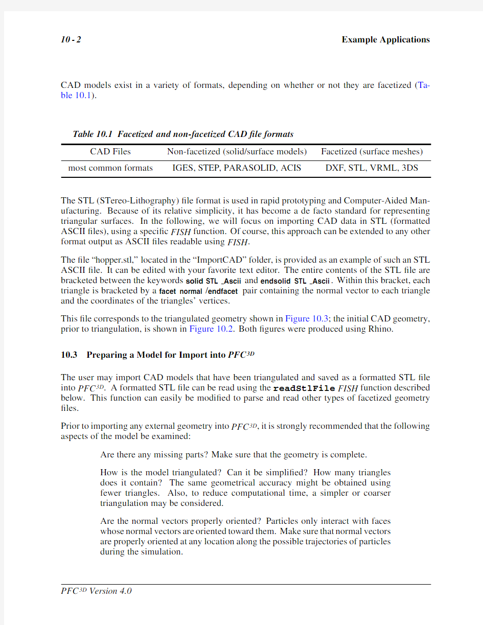
CAD models exist in a variety of formats,depending on whether or not they are facetized(Ta-ble10.1).
Table10.1Facetized and non-facetized CAD?le formats
CAD Files Non-facetized(solid/surface models)Facetized(surface meshes) most common formats IGES,STEP,PARASOLID,ACIS DXF,STL,VRML,3DS
The STL(STereo-Lithography)?le format is used in rapid prototyping and Computer-Aided Man-ufacturing.Because of its relative simplicity,it has become a de facto standard for representing triangular surfaces.In the following,we will focus on importing CAD data in STL(formatted ASCII?les),using a speci?c FISH function.Of course,this approach can be extended to any other format output as ASCII?les readable using FISH.
The?le“hopper.stl,”located in the“ImportCAD”folder,is provided as an example of such an STL ASCII?le.It can be edited with your favorite text editor.The entire contents of the STL?le are bracketed between the keywords solid STL Ascii and endsolid STL Ascii.Within this bracket,each triangle is bracketed by a facet normal/endfacet pair containing the normal vector to each triangle and the coordinates of the triangles’vertices.
This?le corresponds to the triangulated geometry shown in Figure10.3;the initial CAD geometry, prior to triangulation,is shown in Figure10.2.Both?gures were produced using Rhino.
10.3Preparing a Model for Import into PFC3D
The user may import CAD models that have been triangulated and saved as a formatted STL?le into PFC3D.A formatted STL?le can be read using the readStlFile FISH function described below.This function can easily be modi?ed to parse and read other types of facetized geometry ?les.
Prior to importing any external geometry into PFC3D,it is strongly recommended that the following aspects of the model be examined:
Are there any missing parts?Make sure that the geometry is complete.
How is the model triangulated?Can it be simpli?ed?How many triangles
does it contain?The same geometrical accuracy might be obtained using
fewer triangles.Also,to reduce computational time,a simpler or coarser
triangulation may be considered.
Are the normal vectors properly oriented?Particles only interact with faces
whose normal vectors are oriented toward them.Make sure that normal vectors
are properly oriented at any location along the possible trajectories of particles
during the simulation.
The last two items are illustrated in the following.The best way to examine a model is to use a CAD tool and visually inspect the content of the model,check for missing or duplicate parts, weed out irrelevant details or parts that are not likely to come into contact with particles,and check the orientation of the normals prior to saving the model as a formatted STL?le.Please note that particles only“see”walls if the wall normal is pointing at them;if not,they will pass right through them.
10.3.1Model Simpli?cation
An imported model may be large and https://www.doczj.com/doc/f97471071.html,ing it directly may require prohibitively large computational resources because of the large number of triangles involved.It is recommended that the model be simpli?ed to remove details irrelevant to the PFC3D simulation.
For instance,Figure10.1(left)shows a model of a stirred tank reactor in which the tank wall has a certain thickness.In simulating the mixing of particles,the outer wall is irrelevant since it never interacts with particles.Figure10.1(right)shows the same model where only the inner wall of the tank has been kept.
Figure10.1Original model with thick walls(left)and simpli?ed model(right)
10.3.2Model Triangulation
A solid model represents a mathematical description of the entities it contains.Surfaces must be triangulated before they can be read as wall elements into PFC3D.Most CAD systems allow the user to choose how?nely a surface is to be triangulated.The most common measure of how?nely a surface is triangulated is chord error or offset.
Figure10.2shows the CAD de?nition of a hopper prior to triangulation.
Figure10.2CAD model of hopper
Figure10.3is the result of triangulating the CAD de?nition with a chord error of0.1.The resulting surface mesh contains64triangles.
Figure10.3Triangulation with a chord error of0.1results in64triangles
Figure10.4represents the same object triangulated with a chord error of0.001.The total number of triangles is now4680.Clearly,a slight degradation in geometrical accuracy can cause a substantial (almost100-fold)decrease in the number of wall elements,and results in a signi?cant speed-up of the simulation.
Figure10.4Triangulation with a chord error of0.001results in4680triangles Also,the same geometrical accuracy may sometimes be obtained with fewer triangles,as illustrated in Figure10.5:the triangulation on the right-hand side contains fewer triangles than the triangulation on the left-hand side,although no geometrical information is lost in this simpli?cation.
Figure10.5The triangulation on the right contains fewer triangles than the
one on the left,but without any loss of geometrical accuracy
10.3.3Checking Normal Orientation
In PFC3D,the orientation of the walls determines the side the particles will interact with.A particle will pass through a wall if the wall normal does not point toward it.Figure10.6(left)shows the original normal vectors of each triangle in the model(each normal is represented at the center of gravity of each triangle).As a consequence of the original orientation of the various lines used in the construction of the surface,certain surfaces may be oriented differently.Prior to saving the triangulated surface,all triangles must be oriented in a coherent fashion so that normals point toward the particles.Figure10.6(right)shows the results of such a modi?cation.
Figure10.6Normal orientations before and after correction.Triangle nor-
mals are incorrectly oriented(left).All normals point toward the
particles(right).
10.4Importing a CAD Geometry into PFC3D
As mentioned above,here we focus on the importation of CAD data in the STL format,and illustrate this functionality with several example applications.Each example application uses speci?c STL ?les and FISH data?les located in a corresponding sub-folder of the“ImportCAD”folder.However, the STL import functionality,as well as other shared FISH functions,are implemented in the?le “CAD support.?s,”located in the folder“ImportCAD.”This?le is shown in Example10.1: Example10.1CAD import support FISH function
;fname:CAD_support.fis
;
;Itasca Consulting Group,Inc.
;====================================================================== ;Support functions for CAD Examples for PFC3D
;
;-------------------------------------------
;----------------STL Support functions-------------
;----------
;setArray
;----------
def setArray
array arr(60000)xtri(19000,3)ytri(19000,3)ztri(19000,3) end
;----------
;Reads an ASCII STL file composed of triangles
;----------
def readStlFile
wl_=max_wid
command
set echo off
end_command
oo=open(fn_stl,0,1)
nret=read(arr,60000)
oo=out(’Lines input=’+string(nret))
oo=close
ntri=0
loop n(1,nret)
if InTriangle=1
if parse(arr(n),1)=’vertex’
nver=nver+1
xtri(ntri,nver)=parse(arr(n),2)
ytri(ntri,nver)=parse(arr(n),3)
ztri(ntri,nver)=parse(arr(n),4)
endif
if parse(arr(n),1)=’endloop’
InTriangle=0
endif
else
if parse(arr(n),1)=’outer’
InTriangle=1
ntri=ntri+1
nver=0
endif
endif
endLoop
oo=out(’Triangles=’+string(ntri))
loop n(1,ntri)
x1=xtri(n,1)
y1=ytri(n,1)
z1=ztri(n,1)
x_=x1
y_=y1
z_=z1
getMaxMin
x2=xtri(n,2)
y2=ytri(n,2)
z2=ztri(n,2)
x_=x2
y_=y2
z_=z2
getMaxMin
x3=xtri(n,3)
y3=ytri(n,3)
z3=ztri(n,3)
x_=x3
y_=y3
z_=z3
getMaxMin
command
wall face x1y1z1x2y2z2x3y3z3
endCommand
endLoop
command
set echo on
end_command
;Below,we associate the color wcolor_to all the walls of the newly ;read object
wu_=max_wid
_iniWallColor
wcolor_=wcolor_+1
end
;-----------
;getMaxMin
;-----------
def getMaxMin
if x_>x_max
x_max=x_
end_if
if y_>y_max
y_max=y_
end_if
if z_>z_max
z_max=z_
end_if
if x_ x_min=x_ end_if if y_ y_min=y_ end_if if z_ z_min=z_ end_if end ;----------- ;_iniWallColor ;----------- def_iniWallColor wu_=wu_ wl_=wl_ wcolor_=wcolor_ wp_=wall_head loop while wp_#null if w_id(wp_)<=wu_ if w_id(wp_)>wl_ w_color(wp_)=wcolor_ endif endif wp_=w_next(wp_) endloop end ;----------------Simulation Support functions------------- def simini command set random ;set local damping to zero in order to allow unimpeded free flight damp default local0.0 ;activate viscous damping damp default viscous normal0.7notens on shear0.7 ;When PFC3D knows that there will be no more than20,000balls,it ;can optimize its search algorithm accordingly set max_balls20000 ;PFC3D won’t stop with an error message if it cannot pack all the ;balls we are asking it to generate set gen_error off end_command filename=’test’ time_sav=0. dt_sav= 1.0e-1 end def simloop msg=’The simulation will now start and\ncreate a number of SAV files.’msg=msg+’\nThese files can then be used by\nPFC3D or Iv to generate animations.’ o=msgbox(msg,’Start of simulation’,1) loop_i(0,500) if_i<10 _zeros=’000’ else if_i<100 _zeros=’00’ else _zeros=’0’ endif endif _file=string(filename)+string(_zeros)+string(_i) command ;setting ratio to a small value forces PFC3D to continue stepping in ;time until time_sav is reached solve time time_sav ratio 1.0e-8 colorBallsBasedOnVelocity save_file endcommand time_sav=time_sav+dt_sav endloop end def_iniWallVel command wall prop x0.y0.z0. set echo off end_command wp_=wall_head loop while wp_#null if w_color(wp_)=0 wid=w_id(wp_) w_xvel(wp_)=wxvel_ w_yvel(wp_)=wyvel_ w_zvel(wp_)=wzvel_ w_rxvel(wp_)=wrxvel_ w_ryvel(wp_)=wryvel_ w_rzvel(wp_)=wrzvel_ endif wp_=w_next(wp_) endloop command set echo on end_command end ;----------------Plotting Support functions------------- def colorBallsBasedOnVelocity if flg_colorBallsBasedOnVel#0then vmin=0. vmax=2 bp_=ball_head loop while bp_#null bvmag=b_xvel(bp_)*b_xvel(bp_) bvmag=bvmag+b_yvel(bp_)*b_yvel(bp_) bvmag=bvmag+b_zvel(bp_)*b_zvel(bp_) bvmag=sqrt(bvmag) b_color(bp_)=int(((bvmag-vmin)/vmax)*16.) bp_=b_next(bp_) endloop endif end ;----------- ;plotWalls ;----------- def plotWalls wcolor_last=wcolor_-1 loop counter_(0,wcolor_last-1) command pl add wall range col counter_ end_command endloop command pl add wall range col wcolor_last transp80 end_command end define plot_view command plot create the_system end_command plotWalls command pl add ball orange lgreen pl set perspective off pl set background white pl set caption off pl show end_command end ;====================================================================== ;EoF:CAD_support.fis The FISH function readStlFile parses and reads formatted STL?les.Each call to this function, in turn,calls iniWallColor,which assigns a different color to the part that is read so that,later on,color can either be used as a range criterion to assign distinct attributes or kinematics to each wall,or to represent various parts with different levels of transparency or color. In Section10.4.1,we will illustrate and detail the use of the functions implemented in “CAD support.?s”for the case of a stirred tank reactor application.Since the structures of the?les used for the additional examples are the same,these examples will not be discussed in detail. Note that,for purposes of illustration,the number of balls generated in these examples is kept low. These data?les should be modi?ed according to the requirements of each problem. 10.4.1A Stirred Tank Reactor A stirred tank reactor(Figure10.1)is an industrial-size beaker used in the chemical industry to produce compounds through continuous mixing of several chemical reactants.The simpli?ed reactor used in this example is made of two parts:a tank,which is?xed(stator),and a rotating part (rotor)composed of four baf?es. The stirred-tank reactor model is?rst simpli?ed and triangulated in Rhino,which is the CAD tool used in this project.The normal orientations are checked,and the?xed and rotating components of the reactor are saved as two separate STL?les:“STRSTATOR.STL”and“STRROTOR.STL.”The simulation is driven by the data?le“STR.DAT”(Example10.2). The simulation is initialized by calling simini,implemented in“CAD support.?s.”General conditions for the simulation are set therein.All of the situations presented here are dynamic. Therefore,local damping is turned off,and viscous damping at contacts is used to dissipate energy. An estimate of the maximum number of balls is speci?ed to help optimize the PFC3D search algorithm,and gen error is turned off to ensure that the calculation does not stop due to any error during ball generation. “STRSTATOR.STL”is read?rst,followed by“STRROTOR.STL.”As each component is read into PFC3D,a unique color is assigned to it so that it can be identi?ed through a color range function later on.The kinematics of the rotor are prescribed through a call to iniWallVel. Balls are created with a call to makeAssembly(which is speci?c for each example,and therefore implemented directly in“STR.dat”),and ball and wall properties are set. Finally,ball and wall properties are set,and a rotation speed equal to1/2turn per second is imposed around the vertical axis. The actual computation is done by calling simloop.Calculations are done in chunks of dt sav seconds,followed by the output of a save?le.The resulting save?les will be post-processed with Iv.The parameter ratio 1.0e-8is used in the SOLVE command to make sure that SOLVE does not stop prematurely,before dt sav is completed. Figure10.7shows a snapshot of the simulation.The original rotor design is shown in Fig-ure10.8(left).An additional STL?le,“STRROTOR2.STL,”representing a different design(Fig-ure10.8(right)),is also included,and can be substituted in place of“STRROTOR.STL.” Example10.2Main routine of“STR.DAT” ;fname:STR.DAT ; ;Itasca Consulting Group,Inc. ;====================================================================== ;Importing CAD geometry data in PFC3D ;Stirred Tank Reactor example ;------------------------------------------- new ;Load support function call../CAD_support.fis ;-------------- ;makeAssembly ;-------------- def makeAssembly dens_b=1000.0 s_stiff= 2.0e7 n_stiff= 2.0e7 s_stiffw= 2.0e7 n_stiffw= 2.0e7 x_min=0.65 x_max= 2.15 y_min=0.65 y_max= 2.15 z_min=-2.29 z_max= 2.29 r1=0.075 ;---Create assembly--- ;We create4set of balls in2colors num1=0 num2=0 num=500 num1=num2+1 num2=num1+num-1 bc=wcolor_ command gen id=num1,num2x=x_min,x_max y=y_min,y_max z=z_min,z_max& rad=r1,r1 prop color bc range id num1num2 end_command temp=x_min x_min=-x_max x_max=-temp num1=num2+1 num2=num1+num-1 command gen id=num1,num2x=x_min,x_max y=y_min,y_max z=z_min,z_max& rad=r1,r1 prop color bc range id num1num2 end_command bc=wcolor_+1 temp=y_min y_min=-y_max y_max=-temp num1=num2+1 num2=num1+num-1 command gen id=num1,num2x=x_min,x_max y=y_min,y_max z=z_min,z_max& rad=r1,r1 prop color bc range id num1num2 end_command temp=x_min x_min=-x_max x_max=-temp num1=num2+1 num2=num1+num-1 command gen id=num1,num2x=x_min,x_max y=y_min,y_max z=z_min,z_max& rad=r1,r1 prop color bc range id num1num2 end_command ii=out(string(num)+’particles were created’) end ;---------------------------MAIN ROUTINE----------------------------- ;initialize the simulation simini ;Read the STL files set fn_stl=’STRrotor.stl’ readStlFile set fn_stl=’STRstator.stl’ readStlFile ;Generate balls makeAssembly prop dens dens_b ks=s_stiff kn=n_stiff fric=0.4 wall prop ks=s_stiffw kn=n_stiffw ;set wall velocity set wxvel_=0.wyvel_=0.wzvel_=0.;translation set wrxvel_=0.wryvel_=0.wrzvel_= 1.57;rotation _iniWallVel ;set gravity set grav00-10.0 ;plot view set pint100 plot_view ;run the simulation loop set dt_sav= 1.0e-1 set flg_colorBallsBasedOnVel=0 simloop ;------------------------------------------- return ;====================================================================== ;EoF:STR.dat Figure10.7Simulation of a stirred tank reactor with PFC3D(“STR.DAT”) Figure10.8Two baf?e designs represented by“STRROTOR.STL”(left)and “STRROTOR2.STL”(right) 10.4.2Additional Examples The following examples are not described in detail.The data?les used to run the simulations have the same structure as“STR.DAT,”described above.The makeAssembly FISH function is speci?c to each case,and thus de?ned in a speci?c data?le.All examples make use of simini and simloop,de?ned in the?le“CAD support.?s.” 10.4.2.1Ball Mill A ball mill is used to grind particles.The following?les are used in this application:“BALLMILL.DAT,”“BALLMILLBODY.STL”and“BALLMILLCAP.STL.”“BALLMILLBODY.DAT”represents the geometry of the mill.“BALLMILLCAP.DAT”is an end cap holding the particles inside the mill.The cap is rendered transparent to make the interior visible.“BALLMILL.DAT”contains a function that colors balls according to the magnitude of velocity (Figure10.9(bottom)). Figure10.9Ball mill(BALLMILL.DAT):the geometry(top)in operation, with balls colored according to the magnitude of their velocity (bottom) 10.4.2.2Blade Mill A blade mill is also used to grind particles.The following?les are used in this application:“BLADEMILL.DAT,”“BLADEMILLSTATOR.STL”and“BLADEMILLROTOR.STL.”Particles are created in two different colors in order to illustrate the mixing process(Figure10.10). Figure10.10Blade mill 10.4.2.3Bulldozer The following?les are used in this application(Figure10.11):“BULLDOZER.DAT,”“BULL-DOZER.STL”and“FLOOR.STL.” Figure10.11Bulldozer
相关主题
文本预览