当前位置：文档之家› sample average approximation and dual decomposition

sample average approximation and dual decomposition

Production,Manufacturing and Logistics

Supply chain design under uncertainty using sample average approximation and dual decomposition q

Peter Schütz a,*,Asgeir Tomasgard a,b ,Shabbir Ahmed c

Department of Industrial Economics and Technology Management,Norwegian University of Science and Technology,7491Trondheim,Norway b

SINTEF Technology &Society,7465Trondheim,Norway c

School of Industrial and Systems Engineering,Georgia Institute of Technology,Atlanta,GA 30332,USA

a r t i c l e i n f o Article history:

Received 4October 2007Accepted 21November 2008

Available online 7December 2008Keywords:

Supply chain design

Stochastic programming

Sample average approximation Dual decomposition

a b s t r a c t

We present a supply chain design problem modeled as a sequence of splitting and combining processes.We formulate the problem as a two-stage stochastic program.The ?rst-stage decisions are strategic loca-tion decisions,whereas the second stage consists of operational decisions.The objective is to minimize the sum of investment costs and expected costs of operating the supply chain.In particular the model emphasizes the importance of operational ?exibility when making strategic decisions.For that reason short-term uncertainty is considered as well as long-term uncertainty.The real-world case used to illus-trate the model is from the Norwegian meat industry.We solve the problem by sample average approx-imation in combination with dual https://www.doczj.com/doc/ef17133947.html,putational results are presented for different sample sizes and different levels of data aggregation in the second stage.

1.Introduction

Supply chain management includes design of,planning for and operation of a network of suppliers,production facilities,warehouses,and distribution centers in order to satisfy customer demand.Strategic decisions regarding the design of supply chains affect the ability to ef?ciently serve customer demand.The design decisions should therefore not be taken without considering the effect on the operational decisions (Lee and Billington,1992).In this paper we examine the impact different modeling choices of the supply chain operations have on the strategic decisions regarding its design and structure.

The importance of supply chain design was recognized already in the early 1970s (see,e.g.Geoffrion and Graves,1974).The early mod-els however assume the parameters that in?uence the design decisions to be deterministic.For long planning horizons this assumption is unlikely to hold.Demands,prices for raw materials,components and ?nished products,locations of markets,etc.are usually highly uncer-tain over the lifetime of the supply chain and thus require a supply chain that is robust and ?exible enough to cope with the challenges of a changing environment.These challenges lead to an increased interest in stochastic programming models over the past 10–15years.

Traditionally,the research literature focused on the facility location component of supply chain management.Schütz et al.(2008)is a recent example of the facility location approach with uncertain demand,non-convex,non-concave ?rst-stage costs and convex second-stage costs.For a broader overview over stochastic facility location,we refer to the reviews by Louveaux (1993)and Snyder (2006).

We consider a model which covers several levels of the supply chain in contrast to the classical one level facility location models or location–allocation models.In this class of models,there is less literature on stochastic models.MirHassani et al.(2000)present a solution method for a supply chain design problem under uncertain demand that is based on scenario analysis.They also discuss the use of Benders decomposition in a parallel implementation.Lucas et al.(2001)consider a similar capacity planning problem,but develop a solution meth-od based on Lagrangean relaxation and scenario analysis.In Alonso-Ayuso et al.(2003),a supply chain planning model is presented with binary ?rst-stage decisions and continuous second-stage decisions.They use an algorithmic approach based on branch-and-?x to solve their problem.Alonso-Ayuso et al.(2005)present several models for supply chain design and production planning and scheduling.Differ-ent formulations for the problems are discussed.They also provide computational experience for the supply chain design problem.Santoso et al.(2005)consider a supply chain design problem and a solution method based on sample average approximation (SAA)and Benders

This research is sponsored by the Research Council of Norway through the Smartlog project.The authors also wish to thank Dash Optimization for sponsoring the licenses for the Xpress runtime libraries used in the computational cluster.*Corresponding author.Tel.:+4773551371;fax:+4773590260.

E-mail addresses:peter.schutz@iot.ntnu.no ,peter.schutz@sintef.no (P.Schütz).European Journal of Operational Research 199(2009)

409–419

Contents lists available at ScienceDirect

European Journal of Operational Research

j o u r n a l h o m e p a g e :w w w.e l s e v i e r.c o m /l o c a t e /e j o

https://www.doczj.com/doc/ef17133947.html,putational results from a real-world case are also presented.Our paper extends this literature both in terms of solution method and model scope,as explained below.

Our case is from the Norwegian meat industry,based on cooperation with Nortura (www.nortura.no )and studies the effect on the stra-tegic decisions of including the operation of the supply chain under uncertain and highly variable demand.The case is based on work car-ried out in 2005and 2006in restructuring their production network.In Tomasgard et al.(2005),the operational aspects of the same supply chain are modeled,but no computational results are presented.That paper does not look into strategic decisions regarding locations and capacities;the supply chain structure is ?xed.Schütz et al.(2008)present a stochastic one level facility location model for the same supply chain.There,the operational part is aggregated into a single time period and the model handles only a single commodity and only the ?rst part of the supply chain.

The main contribution of this paper is to model and solve a stochastic multi-commodity supply chain design problem with a detailed description of operational consequences from the strategic decisions.It has the same level of detail on the operational side as Tomasgard et al.(2005)and handles in addition strategic decisions regarding location and capacities at every level in the supply chain.Because de-mand in the meat industry can exhibit huge variations over short periods,the supply chain is not only subject to long-term demand uncer-tainty,but also considerable short-term demand uncertainty.The long-term uncertainty covers trends and the development of national demand for meat products over a longer time horizon,whereas the short-term uncertainty deals with weekly demand variations.We study in this paper alternative models where the level of detail used to describe the operational decisions varies and discuss the impact on the strategic decisions.To our knowledge,our paper is the ?rst one to examine whether or not the level of aggregation in the second stage affects the ?rst-stage solution in supply chain design models.Our analysis also examines how the use of a stochastic model in?uences the decisions as compared to a deterministic model.

Modeling operational decisions in the second stage increases the model size considerably.For our model we can only solve problem instances with three or four scenarios when using a single processor computer with 6gigabyte of memory.To solve the model we combine sample average approximation (SAA)(Kleywegt et al.,2001)with dual decomposition (Car?e and Schultz,1999).A second contribution of the paper is therefore to investigate how the approach of combining SAA with dual decomposition scales when distributed processing on a higher number of processors is used to increase the number of scenarios in the formulation.We also examine if increasing the number of scenarios have effect on the quality of the ?rst-stage solution.

In Section 2,we present a supply chain model for the Norwegian meat industry.The scenario generation procedure and the different cases for uncertain demand are discussed in Section 3.In Section 4,we then give a generalized two-stage stochastic programming formu-lation for a supply chain design problem where the supply chain is modeled as a sequence of splitting and combing processes.The solution scheme is presented in Section https://www.doczj.com/doc/ef17133947.html,putational results and an analysis of these results follow in Section 6.We conclude in Section 7.2.The supply chain

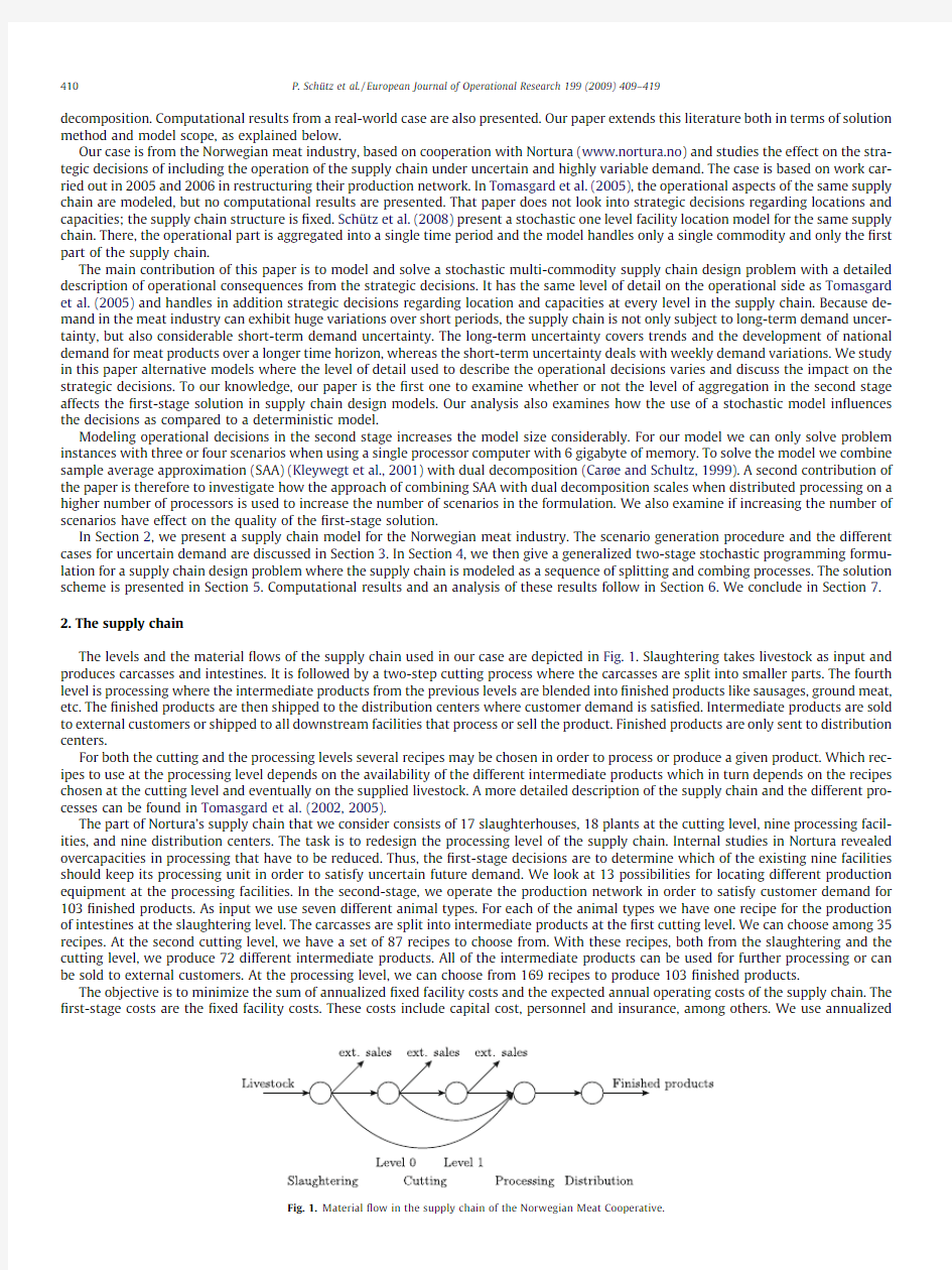
The levels and the material ?ows of the supply chain used in our case are depicted in Fig.1.Slaughtering takes livestock as input and produces carcasses and intestines.It is followed by a two-step cutting process where the carcasses are split into smaller parts.The fourth level is processing where the intermediate products from the previous levels are blended into ?nished products like sausages,ground meat,etc.The ?nished products are then shipped to the distribution centers where customer demand is satis?ed.Intermediate products are sold to external customers or shipped to all downstream facilities that process or sell the product.Finished products are only sent to distribution centers.

For both the cutting and the processing levels several recipes may be chosen in order to process or produce a given product.Which rec-ipes to use at the processing level depends on the availability of the different intermediate products which in turn depends on the recipes chosen at the cutting level and eventually on the supplied livestock.A more detailed description of the supply chain and the different pro-cesses can be found in Tomasgard et al.(2002,2005).

The part of Nortura’s supply chain that we consider consists of 17slaughterhouses,18plants at the cutting level,nine processing facil-ities,and nine distribution centers.The task is to redesign the processing level of the supply chain.Internal studies in Nortura revealed overcapacities in processing that have to be reduced.Thus,the ?rst-stage decisions are to determine which of the existing nine facilities should keep its processing unit in order to satisfy uncertain future demand.We look at 13possibilities for locating different production equipment at the processing facilities.In the second-stage,we operate the production network in order to satisfy customer demand for 103?nished products.As input we use seven different animal types.For each of the animal types we have one recipe for the production of intestines at the slaughtering level.The carcasses are split into intermediate products at the ?rst cutting level.We can choose among 35recipes.At the second cutting level,we have a set of 87recipes to choose from.With these recipes,both from the slaughtering and the cutting level,we produce 72different intermediate products.All of the intermediate products can be used for further processing or can be sold to external customers.At the processing level,we can choose from 169recipes to produce 103?nished products.

The objective is to minimize the sum of annualized ?xed facility costs and the expected annual operating costs of the supply chain.The ?rst-stage costs are the ?xed facility costs.These costs include capital cost,personnel and insurance,among others.We use

annualized

410P.Schütz et al./European Journal of Operational Research 199(2009)409–419

?xed costs in order to be able to compare them with the operating costs in the second stage.For our problem instances,the second-stage costs cover the variable costs of one year operating the production network.The operating costs include production,transportation,and shortfall costs.Production costs cover both direct and indirect costs like ingredients,packaging,personnel,and energy.The transportation costs are given by contracts between Nortura and the different transportation companies.They depend both on origin and destination as well as the pallet type used for transporting the products.

Our supply chain has as a set of facilities or plants which are possible locations for different production processes.The production pro-cesses can be different production lines,technologies or production phases.A production process is either a splitting processes or a combin-ing https://www.doczj.com/doc/ef17133947.html,bining processes are common in manufacturing and assembling and often described by means of a bill of material (BoM).The BoM lists which and how many input products p i are needed to produce one unit of output product p o (see Fig.2a).The splitting pro-cesses are described in a similar manner.The process industry (e.g.the chemical and petroleum industry)uses a so-called reversed bill of material (rBoM)that de?nes in which output products p o a unit of input product p i can be split (see Fig.2b).The meat processing industry can be seen as an example of a supply chain consisting of subsequent splitting and combining processes (see,e.g.Tomasgard et al.,2002,2005).Our formulation allows for choosing from different BoMs for the same process.In our model,each BoM is assigned to the production of one speci?c output product in one speci?c process.Correspondingly each rBoM is assigned to the processing of one speci?c input product.For each location in our supply chain model we will have a set of possible production processes and for each process,a set of possible products.3.Modeling uncertainty

Here we describe the modeling of short-term and long-term uncertainty,the temporal structure of the second-stage and the different demand cases.

3.1.Short-term vs.long-term uncertainty

One of the main purposes of our analysis is to examine the importance of modeling the short-term operations and corresponding de-mand uncertainty when making strategic decisions.There can be high variations in weekly demand for meat products over the year.The products we consider in our problem instances belong to three different product groups.Weekly demand per product group is shown in Fig.3.We see that demand per product group changes by as much as 50%within 1–2weeks,demand for a single product as used in our problem may exhibit even greater variations.

We refer to weekly changes in demand as short-term variations.Some of the variations are due to seasonal changes in the demand pat-tern,but also daily variations,for example due to weather,can have a signi?cant impact on demand.These short-term variations are ne-glected when demand is aggregated in longer time periods (or even a single period)in the second stage.The term long-term uncertainty is used to describe changes in the total level of demand over a longer time horizon like 5–10years.This uncertainty is for example the market share of the company,the total market size or trends in demand for meat products.

In order to study the effect of short-term uncertainty and operational decisions on the strategic decisions,we have to generate scenarios for the short-term demand.We then combine these scenarios with scenarios for changes in the total demand level,i.e.the long-term uncer-tainty.The methods used to generate the demand scenarios are described

below.

P.Schütz et al./European Journal of Operational Research 199(2009)409–419411

Short-term supply chain planning is based on demand forecasts.To capture the short-term uncertainty we use a methodology that com-bines forecasting and scenario-generation (Nowak et al.,2007).We will brie?y describe the steps for the short-term scenario generation here:

(1)For each product,we parametrize an autoregressive process of N th order,AR(N )-process,on historical data (see,e.g.Hamilton,1994).

For our problem instances,we use an AR(1)-process.

(2)We then ?nd the distribution of the historical prediction error for each product.We assume that the error term for a given product is

i.i.d.between different time periods.The historically observed prediction errors then give us a multivariate discrete distribution for all the products’error terms.

(3)On this empirical distribution,we perform a principal component analysis.For the P products we get P principal components and

sort them by the share of variance they explain for the error distribution.

(4)We calculate the ?rst four moments of the empirical distribution of these principal components and choose the K principal compo-nents explaining the highest part of variance as stochastic in the further scenario generation process.For the P àK remaining com-ponents we use their expected value.

(5)We then generate S scenarios for the K stochastic principal components using a moment matching procedure ensuring that the ?rst

four moments in the scenarios are the same as in the historical distribution.The scenarios are equally likely.The method used here is a modi?ed version of the method developed by H?yland et al.(2003).

(6)The scenarios for the principal components are then transformed back into scenarios for the prediction error.

(7)Finally,we combine the forecasting method with the scenario tree for the prediction error to get demand scenarios rather than pure

prediction error scenarios.This procedure is illustrated in detail in Fig.4:Using a deterministic AR(N )-process as forecasting method,

predicted demand in period t +1is given by the formula ^x t t1?a tP N

i ?1b i x t t1ài .In our case,we add a realization of the error term

s t t1as represented in the scenario tree to the ?rst prediction.Thus,the ?rst prediction ^x s t t1?a tP N

i ?1b i x t t1ài t s t t1is based on his-torical data and the error scenario s t t1.When demand for several periods is predicted,the prediction may be based on both historical

demand,predicted demand,and the error scenarios as shown in Fig.4.The advantage of this method is that correlations between stochastic variables are taken care of through principal component analysis.Also,the principal component analysis makes it possible to reduce the number of stochastic variables used.In our case by using 150prin-cipal components for 821stochastic variables we still explain 93%of the variance in the multivariate error distribution.

For the long-term uncertainty we choose a different approach.For reasons of simpli?cation,we model a possible change in long-term demand level without differentiating between the different demand regions.We also assume that an increase in total demand and a de-crease in total demand are equally likely.We use a uniform distribution to describe the demand level,with todays demand as the expec-tation.The scenarios for long-term uncertainty are generated by sampling a factor from a uniform distribution on [0.5;1.5].By multiplying this factor with the demand in any demand scenario we model a change in the long-term demand level.Alternatively,a long-term trend,for example a general increase or decrease in demand level,would be easy to model by changing the interval.3.2.Demand uncertainty

To properly catch all weekly demand variations,one would have to model the second-stage with 52time periods.However,due to restrictions in both solution time and model size,this is not practical.We have to reduce the number of time periods in the second-stage by aggregating them while ensuring that we capture the effect of short-term demand variations.

Demand in the Norwegian meat market follows typical seasonal patterns:during the summer months,demand for barbecue products increases and both Easter and Christmas have distinct demand patterns.We therefore split the year in four seasons,each three

months

412P.Schütz et al./European Journal of Operational Research 199(2009)409–419

https://www.doczj.com/doc/ef17133947.html,ually,there is no correlation in demand between different seasons.We aggregate the ?rst two months of each season into one per-iod and model the last month of each season with a weekly time resolution (four weeks).This way,we capture the weekly demand vari-ations around Easter,early and late summer,and Christmas in detail.

We describe here the problem instances based on three criteria:long-term uncertainty,short-term uncertainty,and aggregation.STU The ?rst problem instance we use is only taking short-term uncertainty into consideration.We choose to generate 200scenarios for

each of the four-week periods using the scenario generation method described above.As we assume no temporal correlation between the different quarters,we can use any combination of these scenarios,resulting in a total of 2004possible demand scenar-ios.Demand in the cumulated two-month periods is represented by its expected value.No long-term uncertainty is modeled.

LTU The second case only takes long-term uncertainty into account.We use expected weekly demand to represent the demand variations

over the year.This demand data is then multiplied with a random factor drawn from a uniform distribution on [0.5;1.5]to model the long-term changes in demand level.The scenarios may be viewed as possible demand realization at a point in the future where all scenarios are equally likely.Alternatively the scenarios may be viewed as realizations of yearly demand over a set of years.No short-term uncertainty is modeled.

LSTU The third case is a combination of long-term and short-term uncertainty.We use the scenario tree from STU and multiply each sce-nario with a random factor that is uniformly distributed on [0.5;1.5].This way,we capture both effects.For each of these non-aggregated cases,we de?ne a corresponding aggregated problem instances.In these aggregated problem in-stances (ASTU,ALTU,and ALSTU),we replace the 20-period second stage problem by a single period problem.All demand,supply,and capacities are cumulated.4.Optimization model

Let us introduce the following notation for our two-stage stochastic programming formulation: Sets F c set of possible facility locations for combining processes F s set of possible facility locations for splitting processes W set of possible warehouse locations

L set of all possible locations,L ?F c [F s [W C set of customer locations

U ej Tset of upstream locations able to send products to location j ,j 2L [C

D ej Tset of downstream locations able to receive products from location j ,j 2L O c ej Tset of combining processes that can be performed at location j ,j 2F c O s ej Tset of splitting processes that can be performed at location j ,j 2F s O ej Tset of all processes that can be performed at location j ,j 2L ,O ej T?O c ej T[O s ej TO set of all processes,O ?S j 2L O ej TP set of products

P i eo Tset of input products for process o ,o 2O P o eo Tset of output products of process o ,o 2O

B eo ;p Tset of (reversed)bills of materials that can be used for processing product p in process o ,o 2O ;p 2P S set of scenarios T

set of time periods

Indices and superscripts o process index,j 2L ;o 2O ej Tb bill of materials index,o 2O ;p 2P ;b 2B eo ;p Tj ,k location indices,j ;k 2L [C p ,q product indices,p ;q 2P s scenario index,s 2S t time period index,t 2T

Parameters,constants,and coef?cients A b p o ;p i

yield of product p o in case one unit p i is processed with reversed bill of materials b ,o 2O s ;p i 2P i eo T;p o 2P o eo T;b 2B eo ;p i TB b p o ;p i amount of product p i needed to produce one unit p o using bill of materials b ,o 2O c ;p i 2P i eo T;p o 2P o eo T;b 2B eo ;p i TC os jt

capacity of process o at location j in scenario s at time t ,j 2F c [F s ;o 2O ;s 2S ;t 2T D ps jt demand for product p at customer location j in scenario s at time t ,j 2C ;p 2P ;s 2S ;t 2T

F o j ?xed cost of locating process o at location j ,j 2F c [F s ;o 2O

H ps jt penalty for not satisfying one unit of demand of product p at customer location j in scenario s at time t ,j 2C ;p 2P ;s 2S ;t 2T P ps jbt cost of processing one unit of product p at location j using (reversed)bill of material b in scenario s time t ,j 2F c [F s ;o 2O ej T;p 2P ;b 2B eo ;p T;s 2S ;t 2T

S ps jt supply of product p at location j in scenario s at time t ,j 2F c [F s ;p 2P ;s 2S ;t 2T

T ps jkt cost of transporting one unit of product p from location j to location k in scenario s at time t ,j 2L ;k 2D ej T;p 2P ,s 2S ;t 2T i ps j 0initial inventory of product p in scenario s at location j ,j 2W ;p 2P ;s 2S p s

probability of scenario s ,s 2S

P.Schütz et al./European Journal of Operational Research 199(2009)409–419413

Decision variables v ps jt inventory of product p at location j in scenario s at period t ,j 2W ;p 2P ;s 2S ;t 2T w ps jkt amount of product p transported from location j to location k in scenario s at time t ,j 2L ;k 2D ej T;p 2P ;s 2S ;t 2T

x ps jbt amount of product p processed/produced at location j using bill of material b in scenario s at time t ,j 2F c [F s ;o 2O ej T,p 2P ;b 2B eo ;p T;s 2S ;t 2T

y o j 1if process o is located at facility location j ,0otherwise,j 2F c [F c ;o 2O ej T

z ps jt

unsatis?ed demand for product p at customer location j in scenario s 2S in period t ,j 2C ;p 2P ;s 2S ;t 2T

We now model our supply chain as two-stage stochastic program with recourse.For reasons of simplicity,we denote the set of feasible combinations of ?rst-stage decisions y o j by Y .The uncertain parameters in this formulation are the costs,supply,capacity,and demand.By n ,we denote the vector of these parameters.For our problem we have n ?eP ;T ;H ;S ;C ;D T,where n s is a given realization of the uncertain parameters

min

X j 2L X

o 2O ej T

F o j y o j t

s 2S

p s Q ey ;n s T

e1T

subject to

y 2Y #f 0;1g j L jáj O j

e2T

with Q ey ;n s Tbeing the solution of the following second-stage problem:

Q ey ;n s T?min

X j 2L X p 2P X

o 2O ej TX b 2B eo ;p TX

t 2T

P ps jbt x ps

jbt tX p 2P X j 2L X k 2D ej TX

t 2T

T ps jkt w ps

jkt t

X p 2P X j 2C X

t 2T

H ps jt z ps

e3T

subject to

S ps jt tX

k 2U ej T

w ps kjt ?X o 2O s ej TX

b 2B eo ;p Tx ps jbt j 2F s ;p 2[

o 2O s ej T

P i eo T;t 2T ;e4TX o 2O s ej TX q 2P i eo TX

b 2B eo ;q T

A b p ;q áx qs

jbt ?

k 2D ej T

w ps jkt

j 2F s ;p 2[

o 2O s ej T

P o eo T;t 2T ;

e5TX

p 2P i eo TX

b 2B eo ;p T

x ps jbt 6C os jt áy o

j 2F s ;o 2O s ej T;t 2T ;e6T

S ps jt tX

k 2U ej T

w ps kjt ?

X o 2O c ej TX q 2P o eo TX

b 2B eo ;q T

B b q ;p áx qs

jbt

j 2F c ;p 2

[

o 2O c ej T

P i eo T;t 2T ;e7TX o 2O c ej TX b 2B eo ;p Tx ps jbt ?X k 2D ej T

w ps jkt j 2F c ;p 2

[

o 2O c ej T

P o eo T;t 2T ;

e8TX

p 2P o eo TX

b 2B eo ;p T

x ps jbt

C os jt

áy o j j 2F c ;o 2O c ej T;t 2T ;e9Tv ps jt à1t

X k 2U ej T

w ps kjt ?v ps

jt t

k 2D ej T

w ps jkt

j 2W ;p 2P ;t 2T ;

e10TX

k 2U ej T

w ps kjt t

z ps jt

D ps jt

j 2C ;p 2P ;t 2T ;

e11Tv ;w ;x ;z P 0

e12T

The objective function (1)is the sum of the ?rst-stage costs and the expected second-stage costs.The ?rst-stage costs represent the costs

of installing a given process at location j .The objective function of the second stage (3)consists of three parts:?rstly,the production costs,secondly,the transportation costs,and thirdly,the shortfall penalty for unsatis?ed demand.Restriction (2)de?nes the feasible set for the binary ?rst-stage variables.Constraints (4)–(6)describe the splitting processes.Constraints (4)ensure that the external supply and all prod-ucts transported into the splitting node are processed.Restrictions (5)force all produced products to be transported to a downstream node.Restrictions (6)limit production to the available capacity in the splitting node.Constraints (7)–(9)describe combining processes in a similar way.Constraints (7)ensure that all products needed in the combining process are supplied at the combining node.Constraints (8)make sure all produced products are transported to downstream nodes and restrictions (9)take care of the capacity restrictions in the combining nodes.Restrictions (10)are the mass balance constraints for the inventory.With Eq.(11),we make sure that the sum of all products transported into a demand node and shortfall is equal to customer demand.Constraints (12)are the non-negativity constraints,the indices are omitted.5.Solution scheme

For the model (1)–(12)off-the-shelf solvers can typically solve instances with 3–4scenarios (the amount of memory is in our experience the limit).A typical problem instance in a practical case would have thousands of scenarios.We handle this using sample average approx-imation (Kleywegt et al.,2001)and dual decomposition (Car?e and Schultz,1999).These procedures are described in the following subsections.

5.1.Sample average approximation

We use sample average approximation (SAA)to reduce the size of problem (1)–(12)by repeatedly solving it with a smaller set of sce-narios.We generate random samples with N

by the sample average function 1

N P N n ?1Q ey ;n n T.The problem (1)–(12)is then approximated by the following SAA problem:

414P.Schütz et al./European Journal of Operational Research 199(2009)409–419

min y 2Y

ey T:?X j 2L X

o 2O ej T

F o j y o

t1N X N n ?1

Q ey ;n n T()

:e13T

The optimal solution of (13),^y

N ,and the optimal value,v N ,converge with probability one to an optimal solution of the original problem (1)–(12)as the sample size increases (Kleywegt et al.,2001).Assuming that the SAA is solved to an optimality gap d P 0,we can estimate the sample size N needed to guarantee an e -optimal solution to the true problem with a probability of at least 1àa as

N P

3r 2max ee àd Tej L jj O jelog 2Tàlog a T

e14T

with e P d and a 2(0,1).

In (14),r 2max is related to the variability of Q ey ?;n Tat the optimal solution y ?

(see Kleywegt et al.(2001)for details).One would in practice choose N taking into account the trade-off between the quality of the solution obtained for the SAA problem and the computational effort needed to solve it.Solving the SAA problem (13)with independent samples repeatedly can be more ef?cient than increasing the sample size N .This procedure can be found in Santoso et al.(2005),but we include it here for the sake of completeness:(1)Generate M independent samples of size N and solve the corresponding SAA

min y 2Y

ey T:?X j 2L

o 2O ej T

F o j y o

j t1N X n

Q ey ;n n T(

)

:We denote the optimal objective function value by v m N and the optimal solution by ^y m N ;m ?1...M .

(2)Compute the average of all optimal objective function values from the SAA problems, v

N ;M and its variance,r 2 v

N ;M : v

N ;M ?1M X

m ?1v m

and

r 2 v

N ;M ?1eM à1TM X M m ?1

ev m N à v N ;M T2

:The average objective function value v

N ;M provides a statistical lower bound on the optimal objective function value for the original problem (1)–(12)(Norkin et al.,1998;Mak et al.,1999).

(3)Pick a feasible ?rst-stage solution y 2Y for problem (1)–(12),e.g.one of the solutions ^y m N .With that solution,estimate the objective

function value of the original problem using a reference sample N 0

N 0e y T:?X j 2L X

o 2O ej T

F o j y o j

t1N 0X N 0

n ?1

Q ey ;n n T:The estimator ~g

N 0e y Tserves as an upper bound on the optimal objective function value.The reference sample N 0is generated indepen-dently of the samples used in the SAA problems.Since the ?rst-stage solution is ?xed,one can choose a greater number of scenarios for N 0than for N as this step only involves the solution of N 0independent second-stage problems (3)–(12).We can estimate the variance of

N 0e y Tas follows:r 2N 0e y T?

eN 0

à1TN 0

X N 0n ?1

X j 2L X

o 2O ej T

F o j y o j tQ ey ;n n

Tà~g N 0e y T

(4)Compute the estimators for the optimality gap and its https://www.doczj.com/doc/ef17133947.html,ing the estimators calculated in steps 2and 3,we get

gap N ;M ;N 0e y

T?~g N 0e y Tà v N ;M and

r 2gap ?r 2N 0e y Ttr 2 v

N ;M :The con?dence interval for the optimality gap is then calculated as

~g N 0e y Tà v N ;M tz a er 2N 0e y Ttr 2 v

N ;M T1=2with z a :?U à1e1àa T,where U (z )is the cumulative distribution function of the standard normal distribution.

5.2.Dual decomposition and Lagrangean relaxation

Step (1)of the SAA algorithm outlined above involves solving a two-stage stochastic mixed-integer problem (13)with N scenarios.Even

though the number of scenarios in this problem is considerably lower than in the original problem (1)–(12),it is still a large problem.To solve each of the SAA problems,we decompose the problem in scenarios (see,e.g.Car?e and Schultz,1999).In order to do this,we intro-duce ?rst-stage variables y 1;...;y n for each scenario n =1,...,N and add non-anticipativity constraints y 1?ááá?y n to the problem (Rock-afellar and Wets,1991).For each j 2L ;o 2O ej T,we implement the non-anticipativity constraints by the equation P N n ?1K n y on

j ?0where K 1?1àN and K n

?1for n =2,...,N .

We de?ne k as the vector of Lagrangean multipliers associated with the non-anticipativity constraints and relax these.The resulting Lagrangean relaxation is

LR ek T?min y 2Y 1X N n ?1X j 2L X o 2O ej T

eF o j y on j tk o j K n y on j TtQ ey n

;n n T !(

)e15T

with Q ey n ;n n Tbeing the solution to the second-stage problem (3)–(12)given realization n of the random parameters.Note that problem (15)

is separable in scenarios.

P.Schütz et al./European Journal of Operational Research 199(2009)409–419415

We ?nd the best lower bound for our problem by solving the Lagrangean dual

LD ?max

LR ek T:

To solve LD ,we use cutting planes (Kelley,1961)in a bundle method with box constraints (see,e.g.Lemaréchal,1986).Let k denote the

superscript for the current iteration and let r k ?P N n ?1K n y

be the subgradient of (15)with respect to k k in iteration k .Further,de?ne L k ?LR ek k Tàk k ár k as the value of (15)without the Lagrangean penalty term.By D we denote the allowed change in the Lagrangean mul-tiplier.The Lagrangean multipliers are then updated solving the following linear problem:

max

k k t1;/

/e16T

subject to

8i ?1;...;k :/6L i tr i ák k t1;e17Tk k t16k k tD ;e18Tk k t1P k k àD ;e19T/2R ;k k t12R j L jáj O j :

e20T

The Langrangean multipliers are optimal once /is no longer changing.To speed up the process of ?nding the optimal Lagrangean multipliers,we solve the single-scenario subproblems only with an optimality gap c P 0in the ?rst iterations.We then reduce c while we proceed with the iterative procedure and eventually solve all the subproblems to optimality.The idea behind this is that the solutions from the ?rst iter-ations provide an initial search direction,whereas we need a better accuracy in the later iterations to determine the optimal value of the multipliers.

The solution y k produced in iteration k is in general not feasible for the SAA problem (13)as the non-anticipativity constraints may be violated.Step (3)of the SAA procedure requires a feasible solution for the original problem (1)–(12),so we use a simple heuristic to turn the infeasible Lagrangean solution into a feasible,but possibly not optimal solution.We generate a feasible solution by ?xing the binary ?rst-stage variables at 1,if they are 1in more than 50%of the optimal single-scenario solutions and 0otherwise.This heuristic may produce feasible solutions far away from the optimal solution,thus increasing the necessary number of iterations.However,it ?nds good enough solutions for our problem instances.Once the ?rst-stage variables are ?xed,we solve the second-stage problem (3)–(12)for each scenario and get an upper bound on the optimal objective function value.5.3.Quality of the solutions

We choose not to solve the Lagrangean subproblems to optimality during the ?rst iterations.During these iterations,we may not get a lower bound on the optimal objective function value.In fact,the calculated lower bound may actually be above the optimal objective func-tion value of the SAA problem.It may also be bigger than the upper bound from a feasible solution.However,we can still guarantee the quality of the feasible solution found.

If we solve all Lagrangean subproblems with an relative optimality gap c P 0and stop the SAA procedure once the relative gap between upper and lower bound estimator is less or equal to P 0,then the feasible solution providing the upper bound is a e tc t c T-optimal solution to the original SAA problem (13).

Let LR c be a the c -optimal upper bound on the solution of the Lagrangean relaxation LR (k )(15).With v N being the optimal objective

function value of (13)and ~g

N 0e y Tbeing an upper bound provided by the feasible solution y ,we get the following three cases:(1)LR c 6v N 6~g

N 0e y T:LR c is a lower bound for v N ,i.e.the solution y providing ~g N 0e y Tis -optimal for the SAA problem.(2)v N 6LR c 6~g

N 0e y T:LR c overestimates v N ,but not by more than c .The difference between LR c and ~g N 0e y Tdoes not exceed ,thus the feasible solution y

is e tc t c T-optimal for the SAA problem.(3)v N 6~g

N 0e y T6LR c :The difference between v N and LR c is at most c .This means,that y is a c -optimal solution for the SAA https://www.doczj.com/doc/ef17133947.html,putational results

The calculations were carried out on a Linux cluster,running kernel 2.6.9with each node consisting of two 1.6GHz Dual-Core Intel Xeon

5110processors and 8GB RAM.The solution scheme is implemented in C++using the library functions of the message passing interface (MPI)for distributed processing and Xpress 2006runtime libraries as solver for the SAA problems.Xpress 2006is also used to solve the linear program updating the Lagrangean multipliers.6.1.Problem instances

We choose to solve all cases using M =20SAA problems.For the SAA problems,we use sample sizes of N =20,40,and 60scenarios.Dual decomposition is combined with a simple heuristic as described in Section 5.2for the non-aggregated cases.The heuristic is used every ?ve iterations to generate a feasible solution to the SAA problem.We stop once the objective function value is within 5%of the lower bound estimator.The best feasible solution of each SAA is then stored as a candidate solution for valuation in the reference sample.For the aggre-gated cases,each SAA problem is solved to optimality,so we store the optimal solutions for evaluation in the reference sample.The size of the reference sample is set to N 0?1000scenarios.

Due to the size of the non-aggregated cases (STU,LTU,and LSTU),we use one processor core per single-scenario subproblem.The single-scenario subproblems have approx.740,000variables and 1650,00constraints.The aggregated problems (ASTU,ALTU,and ALSTU)are

416P.Schütz et al./European Journal of Operational Research 199(2009)409–419

P.Schütz et al./European Journal of Operational Research199(2009)409–419417 much smaller in size,so we can solve stochastic two-stage problems with60scenarios without having to decompose them.The aggregated problems with60scenarios have approx.2,825,000variables and926,000constraints.

Solving the reference sample with a given?rst-stage solution provides a statistical upper bound on the optimal objective function value of the original problem.For the aggregated problem instances,the statistical lower bound is provided by the average of the M optimal objective function values of the SAA problems.

For the disaggregated problem instances,we normally get an optimality gap of less than5%after5–10iterations when using a c-optimal solution of LR(k)to calculate the estimator for the lower bound on the SAA problem.As c>0during these iterations,we cannot guarantee that this estimator is a true lower bound on the optimal objective function value of the SAA problem(see Sections5.2and 5.3).To provide a valid lower bound on the SAA problem and a valid estimate for the optimality gap,we recalculate the lower bound estimator after the SAA procedure is completed using the lower bound on the objective function value of the Lagrangean relaxation.Test runs indicated that this procedure provides good enough solutions considerably faster than using the lower bound on LR(k)directly or solving LR(k)to optimality.

The statistical lower and upper bounds are shown in Table1.We compare the results of the different problem instances with the solu-tion to the expected value problem(EVP),i.e.the solution to the problem where the uncertain parameters are replaced by their expected value.We compute the upper bound provided by the EEV(see,e.g.Birge and Loveaux,1997),the expected value of the EVP solution,by ?nding the expected value of implementing the EVP?rst-stage solution for the different cases.For each disaggregated case,we also give the upper bound when using the solution from the corresponding aggregated case(ASTU,ALTU,and ALSTU).

Firstly,we note that the feasible solutions from the SAA problems give an upper bound that is approx.16%lower than the EEV.The value of the stochastic solution(VSS,see Birge and Loveaux,1997)is at least180mill NOK.Secondly,using the?rst-stage solution from the cor-responding aggregated case as a solution for the disaggregated case works better than the solution from the EVP.However,the solutions for the aggregated case still give expected results that are approx.50mill.NOK worse than the best solutions from the disaggregated cases. Thirdly,the estimator for the lower bound is increasing in the number of scenarios while its variance is decreasing.

In Table2,we present the estimator for the optimality gap as well as the upper and lower limit of the90%-con?dence interval for the best solution from solving the SAA problems with the different sample sizes.The estimator for the optimality gap is calculated by subtract-ing the lower bound(the SAA procedure)from the upper bound(the reference sample).The optimality gap for the EEV and the aggregated cases is calculated using the best lower bound from the SAA problems.

The con?dence interval for the optimality gap is getting narrower as we increase the number of scenarios in the SAA problem.This is mainly due to a smaller variance of the lower bound.Thus,increasing the number of scenarios,we can give a better guarantee with respect to how close we are to the optimal solution.The results for the optimality gap indicate that the solutions produced by our scheme are good enough to be used in a practical application.

The average CPU-time per processor core for solving a single scenario in the SAA problem varies between34min(STU,N=60)and 62min(LTU,N=60).For cases STU and LSTU the CPU-time is slightly decreasing in the number of scenarios,whereas it is slightly increas-ing for case LTU.The CPU-time for the aggregated cases is increasing in the number of scenarios per SAA problem.This is not surprising,as these problems are not decomposed.The CPU-time required for these problems increases for case ASTU from46min(N=20)to206min

Table1

Statistical lower and upper bounds of the SAA problems for M=20and N0?1000.

Case N Lower bound Upper bound

Average r LB Average r UB

STU201,182,82927841,218,2301871 401,185,93128351,217,1201947

601,186,20619201,225,7301946

EEV1,484,7901939

ASTU1,269,5701950

LTU201,288,11137,1071,384,23028,545 401,331,21828,0181,349,84028,158

601,306,37825,9711,381,64029,665

EEV1,630,18030,180

ALTU1,439,33030,175

LSTU201,334,35944,2361,327,40028,671 401,310,12425,2111,340,13028,927

601,314,99522,9011,382,57028,540

EEV1,569,50030,660

ALSTU1,383,14030,595

ASTU201,118,16023961,119,3901653 401,119,70021491,116,7601657

601,119,53014961,116,2501653

EEV1,393,7401670

ALTU201,268,77047,0031,298,21027,811 401,244,49042,3821,301,49028,011

601,277,34024,3301,305,56027,699

EEV1,513,60028,456

ALSTU201,226,48031,0671,235,24028,100 401,249,04035,0421,251,81027,826

601,251,20027,6471,246,13028,574

EEV1,443,54028,875

418P.Schütz et al./European Journal of Operational Research199(2009)409–419

Table2

Estimated optimality gap and con?dence interval with M=20and N0?1000.

Case N Estimated optimality gap90%Con?dence interval

[1000NOK]%r gap Min.%Max.%

STU2035,401 2.99335430,573 2.5840,230 3.40 4031,189 2.63343926,239 2.2136,139 3.05

6039,524 3.33273435,589 3.0043,459 3.66

EEV298,58425.172728294,65724.84302,51225.50

ASTU93,3647.03273779,425 6.7087,3047.36

LTU2096,1197.4646,81728,725 2.23163,51312.69 4018,622 1.4039,722à38,559à2.9075,804 5.69

6075,363 5.7639,42818,504 1.42109,1628.36

EEV298,96222.4641,181239,68218.00358,24326.91

ALTU108,1128.1241,17748,837 3.67167,38812.57

LSTU20à6959à0.5252,715à82,843à6.2168,926 5.17 4030,006 2.2938,371à25,231à1.9385,243 6.51

6067,575 5.1436,59214,899 1.13120,2519.14

EEV235,14117.6253,822157,66211.82312,62023.43

ALSTU48,731 3.6653,785à28,645à2.15126,2079.46

ASTU2012300.112911à2960à0.2654200.48 40à2940à0.262714à6847à0.619670.09

60à3280à0.292229à6489à0.58à71à0.01

EEV274,04024.472721270,12324.12277,95724.82

ALTU2029,440 2.3254,614à49,179à3.88108,0598.52 4057,000 4.5850,802à16,131à1.30130,13110.46

6028,220 2.2136,867à24,851à1.9581,291 6.36

EEV236,26018.5037,439182,36614.28290,15422.72

ALSTU2087600.7141,890à51,543à4.2069,063 5.63 4027700.2244,746à61,643à4.9467,183 5.38

60à5070à0.4139,635à62,125à4.9751,985 4.15

EEV192,34015.3739,852134,97210.79249,70819.96 (N=60),for case ALTU from32min(N=20)to148min(N=60),and from36min(N=20)to166min(N=60)for case ALSTU.Evaluating a given candidate solution in the reference sample requires approximately150min for the disaggregated cases when using20processor cores.The candidate solutions of the aggregated cases need10–15min of CPU-time.

6.2.Solution properties

When we compare the stochastic solutions to the expected value solution,we see that the solutions from the SAA problems open facil-ities with more capacity than the EVP solutions.The solutions of the disaggregated problem instances also install more capacity than the solutions of the aggregated cases.Case LTU is an exception,as the best solution from the SAA problems installs less capacity for ground meat than both the EVP solution and the ALTU solution.In Table3,we show the amount of capacity installed per product group for the solution providing the lowest upper bound for each case.

Opening facilities with more capacity incurs higher?xed costs.The total costs of operating the value chain however are lower for the stochastic solutions that install more capacity.The additional capacity provides a?exibility in the second stage that reduces the expected second-stage costs by more than the?rst-stage costs increase.

One of the purposes of solving several samples in the SAA approach is to?nd good candidates for?rst-stage solutions to be tested in the reference sample.The solution scheme produces19candidate solutions for case STU with N=20and N=40.When we solve this case with N=60,we get18candidate solutions.For case LTU,the number of candidate solutions produced by our heuristic decreases from20for N=20to7when N=60.Case LSTU with combined long-term and short-term uncertainty is solved with20candidate solutions for N=20,15candidate solutions for N=40,and20candidate solutions for N=60.The upper bounds from these candidate solutions do not vary a lot,indicating rather?at objective functions.The solution from the expected value problem however performs poorly in all cases. The aggregated cases are all solved to optimality and produce a single solution over all samples.The optimal solution of the aggregated cases is the same for all problem instances,independent of the number of scenarios or the type of uncertainty modeled.

7.Conclusions

In this paper,we have presented a supply chain design problem from the Norwegian meat industry.The mathematical formulation of the problem can be applied to any supply chain that consists of subsequent levels of splitting and combining processes.It is also possible to adapt the model for supply chains that consist only of splitting processes(e.g.the processing industry)or combining processes(e.g.man-ufacturing and assembly-based industries).We model both detailed operations of the supply chain and aggregated operations in the sec-ond-stage of the problem and examine the effect of this modeling choice on the?rst stage decisions.Due to the size of the non-aggregated problem instances,we use sample average approximation in combination with dual decomposition to solve our https://www.doczj.com/doc/ef17133947.html,paring the results from both types of second-stage models to their corresponding expected value problem,we see that the?rst-stage decisions from the stochastic problems result in considerably lower costs than the solution of the EVP.We also note that the?rst-stage solutions from the aggregated problem instances have higher expected costs than those from the disaggregated problem instances in the disaggregated data-sets,though not as high as the EVP solution.

P.Schütz et al./European Journal of Operational Research199(2009)409–419419

Table3

Installed capacities for the different product groups.

Case Installed capacity(tons/year)

Ground meat Sausages Cold cuts

EVP18,21614,06511,381 STU23,10023,04111,381 LTU17,60023,04111,381 LSTU18,21633,64511,381 AEVP18,21610,6047920 ASTU18,21614,1687920 ALTU18,21614,1687920 ALSTU18,21614,1687920

The results also show that our solution scheme produces good?rst-stage solutions already for small sample sizes in the SAA problem. Increasing the sample size improves the lower bound on the optimal objective function value,thus improving the quality guarantee on the optimality gap.Due to the distributed processing of the solution scheme,we can increase the size of the SAA problems by using more pro-cessors.For our problem instances,we see that increasing the number of scenarios in the SAA problems even reduces the total CPU-time,as the bigger problems produce fewer candidate solutions that have to be evaluated in the reference sample.

Even though we get good solutions for our problem instances,it might be worthwhile to investigate if a more sophisticated heuristic for ?nding feasible solutions produces even better results.We also need to reduce the runtime further in order to include more product fam-ilies and add more facilities to the supply chain design decisions.

For the end-user in the meat industry,variations of this model have been used in the strategy process to examine structural decisions.A traditional supply chain model would not give the same insight as it lacks the operational detail.As the results show:high variations at the operational level will in?uence the strategic decisions.This cannot be captured properly in aggregated models.In addition,even when it comes to pure operational models,we do not know any alternative model that handles a combination of splitting processes and combining processes.This is essential in the meat industry,in order to capture the value creation of the cutting stage and the processing stage.Finally, one of the main advantages for Nortura in practical use has been the ability to examine a set of supply chain con?gurations that are almost equally good.This way,Nortura is more?exible with respect to the future design of the supply chain,knowing that the chosen design might not be optimal,but also that it will not be far away.

References

Alonso-Ayuso,A.,Escudero,L.F.,Garín,A.,Ortu?o,M.T.,Pérez,G.,2003.An approach for strategic supply chain planning under uncertainty based on stochastic0–1 programming.Journal of Global Optimization26(1),97–124.

Alonso-Ayuso,A.,Escudero,L.F.,Ortu?o,M.T.,2005.Modeling production planning and scheduling under uncertainty.In:Ziemba,W.T.,Wallace,S.W.(Eds.),Applications of Stochastic Programming,MPS-SIAM Series on Optimization.Society for Industrial and Applied Mathematics,Philadelphia,PA,pp.217–252(Chapter13).

Birge,J.R.,Loveaux,F.V.,1997.Introduction to Stochastic Programming.Springer-Verlag,New York.

Car?e,C.C.,Schultz,R.,1999.Dual decomposition in stochastic integer programming.Operations Research Letters24(1–2),37–45.

Geoffrion,A.M.,Graves,G.W.,1974.Multicommodity distribution system design by benders decomposition.Management Science20(5),822–844.

Hamilton,J.D.,1994.Time Series Analysis.Princeton University Press,Princeton,NJ.

H?yland,K.,Kaut,M.,Wallace,S.W.,2003.A heuristic for moment-matching scenario https://www.doczj.com/doc/ef17133947.html,putational Optimization and Applications24(2–3),169–185. Kelley,J.E.,1961.The cutting-plane method for solving convex programs.Journal of the Society for Industrial and Applied Mathematics8(4),703–712.

Kleywegt,A.,Shapiro,A.,de Mello,T.H.,2001.The sample average approximation method for stochastic discrete optimization.SIAM Journal on Optimization12(2),479–502. Lee,H.L.,Billington,C.,1992.Managing supply chain inventory:Pitfalls and opportunities.MIT Sloan Management Review33(3),65–73.

Lemaréchal,C.1986.Constructing bundle methods for convex optimization.In:Hiriart-Urruty,J.-B.(Ed.),FERMAT Days85:Mathematics for Optimization,number129in ‘North-Holland Mathematics Studies’,North-Holland,Amsterdam,pp.201–240.

Louveaux,F.V.,1993.Stochastic location analysis.Location Science1(2),127–154.

Lucas,C.,MirHassani,S.A.,Mitra,G.,Poojari,C.A.,2001.An application of Lagrangian relaxation to a capacity planning problem under uncertainty.Journal of the Operational Research Society52(11),1256–1266.

Mak,W.-K.,Morton,D.P.,Wood,R.K.,1999.Monte Carlo bounding techniques for determining solution quality in stochastic programs.Operations Research Letters24(1–2), 47–56.

MirHassani,S.A.,Lucas,C.,Mitra,G.,Messina,E.,Poojari,C.A.,https://www.doczj.com/doc/ef17133947.html,putational solution of capacity planning models under uncertainty.Parallel Computing26(5),511–538.

Norkin,V.I.,P?ug,G.C.,Ruszczyn′ski,A.,1998.A branch and bound method for stochastic global optimization.Mathematical Programming83(3),425–450.

Nowak,M.,Tomasgard,A.,2007.Scenario generation and forecasting,Working paper,Department of Industrial Economics and Technology Management,Norwegian University of Science and Technology,Trondheim,Norway.

Rockafellar,R.T.,Wets,R.J.-B.,1991.Scenarios and policy aggregation in optimization under uncertainty.Mathematics of Operations Research16(1),119–147.

Santoso,T.,Ahmed,S.,Goetschalckx,M.,Shapiro,A.,2005.A stochastic programming approach for supply chain network design under uncertainty.European Journal of Operational Research167(1),96–115.

Schütz,P.,Stougie,L.,Tomasgard,A.,2008.Stochastic facility location with general long-run costs and convex short-run https://www.doczj.com/doc/ef17133947.html,puters and Operations Research35(9), 2988–3000.

Snyder,L.V.,2006.Facility location under uncertainty:A review.IIE Transactions38(7),537–554.

Tomasgard,A.,H?eg,E.,2002.Supply chain optimization and demand forecasting.In:Olhager,J.,Persson,F.,Seldin,E.,Wikner,J.(Eds.),Produktionslogistik2002–Modeller for Effektiv Produktionslogistik,Link?pings tekniske h?gskola.

Tomasgard,A.,H?eg,E.,2005.A supply chain optimization model for the Norwegian meat cooperative.In:Ziemba,W.T.,Wallace,S.W.(Eds.),Applications of Stochastic Programming,MPS-SIAM Series on Optimization,vol.5.Society for Industrial and Applied Mathematics,Philadelphia,PA,pp.253–276(Chapter14).

模拟联合国大会策划案

第四届模拟联合国大会策划书主办：承办：

二O 一三年十月

目录一、活动背景、意义和目标二、所需会议资源三、活动时间及地点四、会议筹备五、模拟联合国大会具体流程六、奖项设置七、经费预算

一、活动背景、意义和目标 1、什么是模拟联合国大会模拟联合国大会是一项国际性的大学生组织和活动，以拓宽学生视野，锻炼学生综合性能力为宗旨，以培养国际性人才为目标，有利于提高大学生组织管理、研究写作、公开发言、与人沟通、求同存异等多面的能力，是一项健康积极、极富教育意义的学生活动。 2、模拟联合国在常理工为丰富我校校园文化，增进我校学生对于当前重大国际议题的理解认识，提高我校学生综合能力，特举办常熟理工学院第三届模拟联合国大会。 3、活动简介学生白由组队、扮演成所代表国的外交官，参与到“联合国会议” 中，按联合国的规则讨论国际热点问题，模拟联合国会议的全过程。模拟联合国中所探讨的涉及人权、环保和社会发展等诸多面的国际议题有助于拓展学生的视野，培养学生以国际眼光看待问题的良好思维模式。同时此次活动以全中文的形式进行，让更多有兴趣的同学能够有机会参与其中。 4、活动目的和意义

哈佛大学全美模拟联合国大会的会议介绍中，第一句话就提至V: “Our primary goal is to provide students interested in exploring the difficulties and complexities of international relations with best possible simulation of diplomacy and negotiation ”。参与模拟联合国活动，最初的目的就是让参与者拥有一种对错综复杂的国际关系的基本认识，伴随着这种认识，参与者将展现出更高水平的外交谈判能力。我们认为，这也就是参与模拟联合国活动的意义和最终目的，即是在对国际社会、间关系有一种基本了解的基础上，能够通过语言表达、文件写作和白身的魅力维护本国利益，达到会议目标。并通过整个的活动，重新认识白己，认识白己的，认识到白己的在将来世界的位置。

《模拟联合国》社团课

《模拟联合国》社团课名称：模拟联合国科目：英语课程类型：选修适合对象：高一、二学生课程开发类型：自编讲义授课教师：卢洋一、课程简介：模拟联合国（Model United Nations，简称MUN）是对联合国以及其它国际组织和机构的会议流程进行模拟的一种活动，简称模联。在模拟联合国会议中，参与者主要是青年学子们，他们扮演各国的外交官，依据联合国及其它国际组织的议事规则，讨论当今国际上的热点问题。作为各国代表，参与者在会议中代表的是一个“国家”（双代表制），在会议主席团的主持和引导下，他们通过演讲阐述“自己国家”的立场和观点，与其它国家的代表沟通与协作，共同解决矛盾与冲突。二、课程意义：模拟联合国社团课的目的在于使青年学生们对联合国的运作方式和议事规则有更加深入的了解，同时通过扮演各国外交官、模拟联合国会议流程、讨论国际热点问题的方式。同时，模拟联合国社团课着重于培养青年学生们进行有效演讲、有效辩论、有效沟通的能力以及锻炼参与者们解决问题的能力。此外，在模拟联合国会议中，各位代表所代表的国家并非是自己真正所属的国家，对其他国家政治、经济、外交政策以及一些具体问题的调研，有助于增进国家之间的理解以及加强对多元文化的认同及包容性。三、课程目标： 1、了解联合国的相关知识及模拟联合国的基本知识； 2、能围绕某一过意热点话题，收集资料，并形成自己的观点，撰写立场文件； 3、掌握辩论和游说的技巧； 4、拓展国际视野、激发学习能力、培养领袖气质和合作精神； 5、培养团队合作精神，培养风度、气质、领导力； 6、提高沟通和表达的能力，增强社会责任感四、课程内容： 1、了解联合国和“模拟联合国”相关知识运用资料和视频简述“模拟联合国”会议的流程和联合国常识；运动资料说明“模拟联合国”会议文件写作要求、时事要点、逻辑分析常识。 2、撰写立场文件简述搜集资料的方法和途径；分小组搜集资料并汇总；举例说明撰写立场文件的方法；根据某一话题独立撰写立场文件。 3、正式会议流程的学习熟悉“模拟联合国”会议的具体流程；辩论技巧及游说技巧的专项学习；草案、修正案的撰写指导；选择话题开展完整的“模拟联合国”会议。五、课程评价：本课程以小组和个人相结合的方式开展评价，以等级制（A、B、C、D）来表示。平时表现包括：1.上课发言和专注情况；2.分工合作情况；3.文件撰写质量； 4.正式活动时的活动表现。

小学数学新课标解读

小学数学新课标解读《全日制义务教育数学课程标准（修定稿）》（以下简称《标准》）是针对我国义务教育阶段的数学教育制定的。根据《义务教育法》.《基础教育课程改革纲要（试行）》的要求，《标准》以全面推进素质教育，培养学生的创新精神和实践能力为宗旨，明确数学课程的性质和地位，阐述数学课程的基本理念和设计思路，提出数学课程目标与内容标准，并对课程实施（教学.评价.教材编写）提出建议。《标准》提出的数学课程理念和目标对义务教育阶段的数学课程与教学具有指导作用，教学内容的选择和教学活动的组织应当遵循这些基本理念和目标。《标准》规定的课程目标和内容标准是义务教育阶段的每一个学生应当达到的基本要求。《标准》是教材编写.教学.评估.和考试命题的依据。在实施过程中，应当遵照《标准》的要求，充分考虑学生发展和在学习过程中表现出的个性差异，因材施教。为使教师更好地理解和把握有关的目标和内容，以利于教学活动的设计和组织，《标准》提供了一些有针对性的案例，供教师在实施过程中参考。二、设计理念数学是研究数量关系和空间形式的科学。数学与人类的活动息息相关，特别是随着计算机技术的飞速发展，数学更加广泛应用于社会生产和日常生活的各个方面。数学作为对客观现象抽象概括而逐渐形成的科学语言与工具，不仅是自然科学和技术科学的基础，而且在社会科学与人文科学中发挥着越来越大的作用。数学是人类文化的重要组成部分，数学素养是现代社会每一个公民所必备的基本素养。数学教育作

为促进学生全面发展教育的重要组成部分，一方面要使学生掌握现代生活和学习中所需要的数学知识与技能，一方面要充分发挥数学在培养人的科学推理和创新思维方面的功能。义务教育阶段的数学课程具有公共基础的地位，要着眼于学生的整体素质的提高，促进学生全面.持续.和谐发展。课程设计要满足学生未来生活.工作和学习的需要，使学生掌握必需的数学基础知识和基本技能，发展学生抽象思维和推理能力，培养应用意识和创新意识，在情感.态度与价值观等方面都要得到发展；要符合数学科学本身的特点.体现数学科学的精神实质；要符合学生的认知规律和心理特征.有利于激发学生的学习兴趣；要在呈现作为知识与技能的数学结果的同时，重视学生已有的经验，让学生体验从实际背景中抽象出数学问题.构建数学模型.得到结果.解决问题的过程。为此，制定了《标准》的基本理念与设计思路。基本理念数学课程应致力于实现义务教育阶段的培养目标，体现基础性.普及性和发展性。义务教育阶段的数学课程要面向全体学生，适应学生个性发展的需要，使得：人人都能获得良好的数学教育，不同的人在数学上得到不同的发展。课程内容既要反映社会的需要.数学学科的特征，也要符合学生的认知规律。它不仅包括数学的结论，也应包括数学结论的形成过程和数学思想方法。课程内容要贴近学生的生活，有利于学生经验.思考与探索。内容的组织要处理好过程与结果的关系，直观与抽象的关系，生活化.情境化与知识系统性的关系。课程内容

模拟联合国大会流程

模拟联合国大会流程委员会结构 Committee Structure 一个委员会由一个主席团（Members of the Dais）负责。主席（The Chair）主持会议，主席的任务是按照联合国正式的程序规则监督并推动会议进程(Oversees Debate and Guides Delegates Through the Rules of Procedure)。会议指导(Director)负责审阅代表提交的会议文件。主席助理(Rapporteur)负责点名、录入发言人名单(Speakers' list)。流程与规则 Rules of Procedures 一、正式辩论 Formal Debate 1、点名 Roll Call 在这一阶段，主席助理会按国家字母顺序依次点出国家名，被点到的国家举起国家牌(Placard)，并回答：“present(到)”。 E.g. The rapporteur: Honorable delegates, now we are going to have the roll call. Those countries called please raise your placards and answer PRESENT. Afghanistan...... 2、确定议题 Setting the Agenda 本次会议将会有两个议题供代表们选择，代表们通过讨论、投票，确定出要首先讨论的议题。在确定议题的阶段，主席分别在赞成首先讨论议题A和赞成首先讨论议题B的国家中，各随机点出3名代表（即，共6名）进行发言，阐述选择先讨论该议题的原因、动机等，发言时间为90秒。6名代表都发言完毕后，将进行投票，投票原则为简单多数，即50％＋1。 E.g. The Chair: Since we have two topic areas, we are going to set the agenda first. Those countries in favor of talking about topic area A first please raise your placards... China, Russia, Singapore, thanks. Those countries in favor of talking

(完整版)心理学研究方法

福建省高等教育自学考试应用心理学专业（独立本科段）《心理学研究方法》课程考试大纲第一部分课程性质与目标《心理学研究方法》是福建省高等教育自学考试应用心理学专业（独立本科段）的一门专业基础必修课程，目的在于帮助考生了解和掌握心理学研究的理论基础和主要方法，检验考生对心理学研究理论基础与主要方法，检验考生对心理学研究方法的基本知识和主要内容的掌握水平与应用能力。心理学研究的对象是心理现象。它的研究主题十分广泛：即涉及人的心理也涉及动物的心理；即涉及个体的心理也涉及群体的心理；即涉及有意识的心理也涉及潜意识的心理；即涉及与生理过程密切相关的心理也涉及与社会文化密切相关的心理。心理学研究是一种以经验的方式对心理现象进行科学探究的活动。由于心理学的研究方法是以经验的或实证的资料为依据的，因而使心理学与哲学相区别，也与人文学科相区别。设置本课程的具体目的要求是，学习和掌握心理学研究方法的基本理论和基本技能，将有助于学生们理解心理学的基本概念、基本原理和基本理论。理解心理学家在探索心理与行动时所做的一切，有助于考生将来为心理学的发展做出有益的贡献。第二部分考核内容与考核目标第一编心理学研究基础第一章心理学与科学一、学习目的与要求通过本章学习，要求考生了解心理学的性质，了解心理学科学研究的方法、特征及基本步骤，理解心理学研究的伦理问题和伦理规范。二、考核知识点与考核目标 1、识记：（1）心理学的含义；（2）心理学科学研究的特征：系统性、重复性、可证伪性和开放性；（3）知情同意。 2、领会：（1）一般人探索世界的常用方法；（2）心理学研究主要包含哪几个步骤；（3）科学研究的开放性主要表现在哪几方面； 3、应用：（1）根据科学研究的特征来分析某些心理学的研究；（2）心理学研究的伦理问题及以人为被试的研究的伦理规范来分析是否可以在心理学研究中使用欺骗的方法。

模拟联合国大会总结

模拟联合国大会总结为了扩展学生的眼界,使学生对国际时事有更多的关注和了解，提高学生的政治修养，我院特举办了第二届模拟联合国大会。 19号19:00，大会准时开始。在介绍了评委和嘉宾后，播放了开幕视频，主席团就座，大会正式开始。主席助理按照国家名单依次点名，共有11个国家出席本次会议。之后，大会主席主持了辩论会。各国家代表团积极参与会议，场面十分热烈，在自由磋商阶段，各国家代表团积极主动的协商，就利比亚战争问题展开了广泛而深入的讨论。从整体上看，本次会议十分成功。会议过程中出现了这样几点可圈可点的地方。第一是主席团很好的主持了本次会议，引导了会议的进程。第二是志愿者辛勤的劳动和热情的服务是本次活动的一大亮点本次会议一共有8名志愿者，他们在会议中负责接待嘉宾评委、传递意向条、维持会场秩序、发放文件、为各位代表提供帮助等工作，很好的阐释了志愿者的奉献精神，他们感动了各代表团的代表。赢得了全场所有人的尊敬和赞赏。第三，各国家代表团的代表在充分准备的基础上积极地参与会议，并且很好的运用了各种会议规则，推动会议走向一个又一个的高潮。代表们能够按照培训中所学到的知识，不断提出动议来推动会议的进程，为本次会议的成功召开作出了代表所应有的贡献。总之，是会议工作人员和各位代表共同努力，促成了本次模拟联

合国大会的成功召开。但在活动过程中也产生了很多的不足。第一是会议前草案的印发不是很仔细，以至于将英国草案印发错误。第二是邀请评委和嘉宾的工作没有安排好。本次活动得到了团委和学生会的大力支持和同学们的积极参与，模拟联合国大会举办的十分成功。活动极大的提高了同学们的实践能力。很多参与者表示，在准备这次会议中，他们对世界都有了一次全新的认识。他们学到了很多关于国家和世界的知识，体会到了作为外交官为国家争取利益的那种国家荣誉感，演讲和辩论水平也得到了很大的提高。工作人员在这次活动中也受益匪浅。主席团、起草委员会、秘书处和志愿者都积极参与到活动中，从会议的筹备工作到会议召开时的各项准备，无不让他们体会到集体协作的力量。也许，这就是他们参与活动最大的收获。

模拟联合国会议规则流程

模拟联合国会议规则流程 1.点名（Roll Call） ?点名的作用：确定到场国家总数，由此计算简单多数（1/2多数）和三分之二多数。这些数据决定了表决通过的标准。 ?点名的方式：主席助理按照国家名单上的顺序点名，点到的国家高举国家牌并答“到(Present) ”。主席助理重复“某某国代表出席”。 2.设定议题（Setting the Agenda） ?设定议题的条件：一个委员会同时有两个或两个以上的议题待讨论。 ?设定议题的目的：确定多数国家感兴趣的议题为优先讨论的议题。 3.正式辩论（Formal Debate） ?辩论的概念：不同于平时的辩论比赛，模联中的发言、磋商、游说等均被视为辩论。 ?正式辩论：按照发言名单顺序进行的辩论叫正式辩论。 ?发言名单(Speakers’ List) ?发言名单的产生：确定议题后，正式辩论开始。主席会请需要发言的代表举国家牌，并随机点出国家名，当代表听到自己国家被点到后，放下国家牌。主席助理同步记录，代表便可在大屏幕上看到发言名单。 ?发言名单的作用：供各国代表根据自己既定的发言主题发表讲话。 ?发言名单的缺点：各讲各的，主题分散，不利于促进共识的形成。 ?追加发言机会（国家名未在发言名单上或已经完成发言），可向主席台传意向条（Page）要求在发言名单上添加其代表国家，主席会将该国家名加在发言名单最后。如代表已在发言名单上并还未发言，则不能追加发言机会。 ?发言时间：每位代表有120秒的初始发言时间（Speaking Time），可通过动议（Motion to Set Speaking Time）更改。 ?让渡：代表在发言时间内结束发言，可将剩余时间让渡 ?让渡给他国代表（Yield Time to Another Delegate）：让渡国A代表和被让渡国B代表协商一致后（传意向条，会前游说等），B代表在A代表剩余的时间内进行发言。如B代表发言结束还有时间剩余，不能再次让渡，主席将继续主持会议。 ?让渡给问题（Yield Time to Questions）：代表将剩余时间让渡给问题，主席会请需要提问的代表举牌，并随机点出代表进行提问，发言代表可在剩余时间内回答任何被提出的问题，提问时间不占用剩余时间，提问内容必须根据发言者的意思来问。这种方式可以体现发言代表的思辨、反应和口语表达能力。 ?让渡给评论（Yield Time to Comments）：代表将剩余时间让渡给评论，主席会请需要评论的代表举牌，并随机点出代表进行评论，让渡者没有权利再一次进行观点

小学数学新课程标准(修改稿——)解读

小学数学新课程标准(修改稿)解读一、前言《全日制义务教育数学课程标准（修改稿）》（以下简称《标准》）是针对我国义务教育阶段的数学教育制定的。根据《义务教育法》、《基础教育课程改革纲要（试行）》的要求，《标准》以全面推进素质教育，培养学生的创新精神和实践能力为宗旨，明确数学课程的性质和地位，阐述数学课程的基本理念和设计思路，提出数学课程目标与内容标准，并对课程实施（教学、评价、教材编写）提出建议。《标准》提出的数学课程理念和目标对义务教育阶段的数学课程与教学具有指导作用，教学内容的选择和教学活动的组织应当遵循这些基本理念和目标。《标准》规定的课程目标和内容标准是义务教育阶段的每一个学生应当达到的基本要求。《标准》是教材编写、教学、评估、和考试命题的依据。在实施过程中，应当遵照《标准》的要求，充分考虑学生发展和在学习过程中表现出的个性差异，因材施教。为使教师更好地理解和把握有关的目标和内容，以利于教学活动的设计和组织，《标准》提供了一些有针对性的案例，供教师在实施过程中参考。二、设计理念数学是研究数量关系和空间形式的科学。数学与人类的活动息息相关，特别是随着计算机技术的飞速发展，数学更加广泛应用于社会生产和日常生活的各个方面。数学作为对客观现象抽象概括而逐渐形成的科学语言与工具，不仅是自然科学和技术科学的基础，而且在社会科学与人文科学中发挥着越来越大的作用。数学是人类文化的重要组成部分，数学素养是现代社会每一个公民所必备的基本素养。数学教育作为促进学生全面发展教育的重要组成部分，一方面要使学生掌握现代生活和学习中所需要的数学知识与技能，一方面要充分发挥数学在培养人的科学推理和创新思维方面的功能义务教育阶段的数学课程具有公共基础的地位，要着眼于学生的整体素质的提高，促进学生全面、持续、和谐发展。课程设计要满足学生未来生活、工作和学习的需要，使学生掌握必需的数学基础知识和基本技能，发展学生抽象思维和推理能力，培养应用意识和创新意识，在情感、态度与价值观等方面都要得到发展；要符合数学科学本身的特点、体现数学科学的精神实质；要符合学生的认知规律和心理特征、有利于激发学生的学习兴趣；要在呈现作为知识与技能的数学结果的同时，重视学生已有的经验，让学生体验从实际背景中抽象出数学问题、构建数学模型、得到结果、解决问题的过程。为此，制定了《标准》的基本理念与设计思路基本理念。（一）总：六大理念 1、人人学有价值的数学，人人都能获得必需的数学，不同的人在数学上得到不同的发展 2、数学是人们生活、劳动和学习必不可少的工具，数学是一切重大技术发展的基础，数学是一种文化。 3、数学学习的内容要有利于学生主动地进行观察、实验、猜测、验证、推理、与交流，动手实践、自主探索与合作交流是学生学习数学的重要方式。 4、学生是数学学习的主人，教师是数学学习的组织者、引导者、合作者。 5、评价的目的—了解学生的数学学习历程，改进教师的教学；目标多元，方法多样；重过程，轻结果；关注情感态度。 6、把现代信息技术作为学生学习数学和解决问题的强有力的工具。（二）分六大理念的解读: 数学课程应致力于实现义务教育阶段的培养目标，体现基础性、普及性和发展性。义务教育阶段的数学课程要面向全体学生，适应学生个性发展的需要，使得：人人都能获得良好的数学教育，不同的人在数学上得到不同的发展。 1、关于数学课程的功能（1）“人人学有价值的数学”是指作为教育内容的数学，应当是适合学生在有限的学习时间里接触、了解和掌握的数学。怎样理解有价值的数学?

全球模拟联合国大会的议事规则

全球模拟联合国大会的议事规则本议事规则将指导全球模拟联合国会议模拟举行大会全体会议和各主要委员会会议。这些规则改编自实际的《联合国大会议事规则》，供全球模拟联合国使用。一、议程常会临时议程第1条全球模拟联合国(模拟联合国)会议的临时议程应由模拟联合国秘书长草拟，至迟于会议开幕前两个月传递给各代表团第2条会议的临时议程应包括： (a)关于为每届会议选定主题的报告； (b)模拟联合国秘书长认为需要向模拟联合国大会提出的所有项目。议程的通过第3条每届会议的临时议程应在会议开幕式上提请模拟联合国大会批准。二、代表团组成第4条

会员国代表团应由不超过六名代表组成。三、大会主席和副主席选举第5条除非模拟联合国大会另有决定，模拟联合国大会应选举主席一人，副主席五人，并至少在由其主持的会议开幕前三个月选出。在选举模拟联合国大会主席和副主席时，应考虑尽可能将这些职务分配给下列区域，以确保模拟联合国总务委员会的代表性：非洲、亚洲、东欧、拉丁美洲和加勒比地区、西欧和其他国家。他们的任期应自当选之日开始，并应在选举出模拟联合国大会下一届会议新的主席团成员时为止。如果某个成员在他或她任期届满之前不再属于模拟联合国总务委员会，应单独举行补选，来为剩余的任期选举一名新成员。临时主席第6条大会主席因故不能出席某次会议或会议的一部分时，应指定副主席一人代行主席职务第7条副主席代理大会主席时，其权力和职责与主席相同。大会主席的一般权力第8条大会主席除行使本规则其他条款所赋予的权力外，应宣布本届会议每次全体会议的开会和散会、主持全体会议的讨论、确保对本规

模拟联合国大会活动策划书(完整版)

策划编号：YT-FS-3912-17 模拟联合国大会活动策划书(完整版) Develop Detailed Rules Based On Expected Needs And Issues. And Make A Written Plan For The Links To Be Carried Out T o Ensure The Smooth Implementation Of The Scheme. 深思远虑目营心匠 Think Far And See, Work Hard At Heart

模拟联合国大会活动策划书(完整版) 备注：该策划书文本主要根据预期的需求和问题为中心，制定具体实施细则，步骤。并对将要进行的环节进行书面的计划，以对每个步骤详细分析，确保方案的顺利执行。文档可根据实际情况进行修改和使用。一．活动主题 “模拟联合国大会”活动二．活动目的旨在通过本次活动来增加同学们对联合国组织的认识，同时培养让大家以国际的眼光来观察问题的能力，提高同学们组织策划管理能力和自身交际能力。三．活动对象电子学院全体学生四．活动时间（1）学院选拔时间：XX.11.18——XX.11.21 （2）全校活动时间：XX.12.5下午1：30 五．活动开展

（一）学院选拔（1）宣传方式：大一新生中到班宣传（2）选拔方式： 1.自己选取一则英语小演讲进行演讲； 2.接受现场评委临场提问之后有评委通过综合评定，选出两名选手代表电子学院参加全校活动。（二）全校活动（1）活动议题：农业发展和食品安全（2）活动目标：激发热情 generating young passion 社会责任 social responsibility 想象创新 imagination for innovation 勇于尝试 willing to try 追求卓越 excellence in execution （3）活动大概：学院自己内部选出两个代表（一个是正外交官，

2011版小学数学课程标准解读(全)

解读《义务教育小学数学课程标准》（2011年版）一【新旧课标比较】与旧课标相比，新课标从基本理念、课程目标、内容标准到实施建议都更加准确、规范、明了和全面。具体变化如下：一、总体框架结构的变化 2001年版分四个部分：前言、课程目标、内容标准和课程实施建议。 2011年版把其中的“内容标准”改为“课程内容”。前言部分由原来的基本理念和设计思路，改为课程基本性质、课程基本理念和课程设计思路三部分。二、关于数学观的变化 2001年版：数学是人们对客观世界定性把握和定量刻画、逐渐抽象概括、形成方法和理论，并进行广泛应用的过程。数学作为一种普遍适用的技术，有助于人们收集、整理、描述信息，建立数学模型，进而解决问题，直接为社会创造价值。 2011年版：数学是研究数量关系和空间形式的科学。数学作为对于客观现象抽象概括而逐渐形成的科学语言与工具。数学是人类文化的重要组成部分，数学素养是现代社会每一个公民应该具备的基本素养。三、基本理念“三句”变“两句”，“6条”改“5条” 2001年版“三句话”：人人学有价值的数学，人人都能获得必需的数学，不同的人在数学上得到不同的发展。 2011年版“两句话”：人人都能获得良好的数学教育，不同的人在数学上得到不同的发展。 “6条”改“5条”：在结构上由原来的6条改为5条，将2001年版的第2条关于对数学的认识整合到理念之前的文字之中，新增了对课程内容的认识，此外，将“数学教学”与“数学学习”合并为数学“教学活动”。 2001年版：数学课程——数学——数学学习——数学教学活动——评价——现代信息技术 2011年版：数学课程——课程内容——教学活动——学习评价——信息技术四、理念中新增加了一些提法要处理好四个关系数学课程基本理念（两句话）数学教学活动的本质要求培养良好的数学学习习惯注重启发式正确看待教师的主导作用处理好评价中的关系

模拟联合国会议主要流程

模拟联合国会议主要流程一、点名 roll call 在这一阶段，主席助理会按国家字母顺序依次点出国家名，被点到的国家举起国家牌(placard)，并回答：present(到)。点名为每一个session都需要做的。二、确定议题 setting agenda 本次会议将会由两个议题供代表们选择，代表们通过讨论、投票，确定出要首先讨论的议题。在确定议题的阶段，主席分别在赞成首先讨论议题A和赞成首先讨论议题B的国家中，各随机点出2名代表（即，共4名）进行发言，发言顺序为一正一反交叉进行。阐述选择先讨论该议题的原因、动机等，发言时间为90秒。4名代表都发言完毕后，将进行投票，投票原则为简单多数,50％＋1。三、发言名单Speakers’ list 代表们确定议题之后，正式辩论开始。主席会请需要发言的代表举国家牌（也就是所有的国家都举牌），并随机读出国家名，代表们发言的顺序即主席点名的顺序，当代表们听到自己国家被点到之后，便放下国家牌。每个代表有120秒的发言时间（初始时间，可更改），代表可在大屏幕上看到发言名单。如果需要追加发言机会（国家名未在发言名单上或已经完成发言），代表可向主席台传意向条(page)要求在发言名单上添加其代表的国家，主席会将该过的名字加在发言名单的最后。如果代表已在发言名单上，并且还没有发言，则不能在其发言之前追加发言机会。一旦发言名单上所有国家已发言，并且没有任何代表追加发言，会议直接进入投票表决阶段。四、让渡时间 yield time

代表在发言时间内结束发言之后，可将剩余时间让渡（让渡时间仅出现在120秒的发言名单中），让渡对象如下： ——让渡给他国代表(yield time to another delegate)这是我们最提倡的一种让渡方式。让渡国a代表和被让渡国b代表私下协商一致后（传意向条，会前游说等），b代表在a代表剩余的时间内进行发言。如果b代表发言结束还有时间剩余，b代表不能将其再次让渡，主席将继续主持会议。 ——让渡给问题(yield time to questions) 一旦代表将剩余时间让渡给问题，主席会请需要提问的代表举牌，并随机点出代表进行提问，提问时间不占用剩余时间，提问内容必须根据发言者的意思来问。发言代表可在剩余时间范围内回答任何被提出的问题，提问不占用时间。这种让渡方式可以体现发言代表的思辩、反应及口语表达能力，但如果代表水平还有一定差距，选择这种让渡方式就是比较不明智的。 ——让渡给评论(yield time to comments) 一旦代表将剩余时间让渡给评论，主席会请需要评论的代表举牌，并随机点出代表进行评论，让渡时间给评论的代表没有权利再一次进行观点的陈述或者对评论进行反驳。这种让渡方式是比较冒风险的。如果发言代表和盟国交涉成功让盟国进行有利评论，且盟国保证他到时会举牌并让主席点到他，这样会对发言代表比较有利。但如果评论机会落入反对国手中，该国将会对发言代表的立场进行反驳及批判，这样就会使发言代表进入比较被动的劣势状态。所以，请代表们慎重选择。 ——让渡给主席(yield time to the chair)

(完整版)人教版四年级数学新课标解读

人教版小学数学四年级下册新课标解读崔庙镇实验小学四年级

人教版小学数学四年级下册新课标解读一、教材的主要内容: 小数的意义与性质，小数的加法和减法，四则运算，运算定律与简便计算，三角形，位置与方向，折线统计图，数学广角和数学综合运用活动等。其中小数的意义与性质，小数的加法和减法，运算定律与简便计算，以及三角形是本册的重点教学内容。二、教材的学习目标 1、理解小数的意义和性质，体会小数在日常生活中的应用，进一步发展数感，掌握小数点位置移动引起小数大小变化的规律，掌握小数的加法和减法。 2、掌握四则混合运算的顺序，会进行简单的整数四则混合运算;探索和理解加法和乘法的运算定律，会应用它们进行一些简便运算，进一步提高计算能力。 3、认识三角形的特性，会根据三角形的边、角特点给三角形分类，知道三角形任意两边之和大于第三边以及三角形的内角和是 180°。 4、初步掌握确定物体位置的方法，能根据方向和距离确定物体的位置，能描述简单的路线图。 5、认识折线统计图，了解折线统计图的特点，初步学会根据统计图和数据进行数据变化趋势的分析，进一步体会统计在现实生活中的作用。

6、经历从实际生活中发现问题、提出问题、解决问题的过程，体会数学在日常生活中的作用，初步形成综合运用数学知识解决问题的能力。 7、了解解决植树问题的思想方法，培养从生活中发现数学问题的意识，初步培养探索解决问题有效方法的能力，初步形成观察、分析及推理的能力。 8、体会学习数学的乐趣，提高学习数学的兴趣，建立学好数学的信心。 9、养成认真作业、书写整洁的良好习惯。三、教材的编写特点: 本册实验教材具有内容丰富、关注学生的经验与体验、体现知识的形成过程、鼓励算法多样化、改变学生的学习方式，体现开放性的教学方法等特点。同时，本实验教材还具有下面几个明显的特点。 1. 改进四则运算的编排，降低学习的难度，促进学生的思维水平的提高。四则运算的知识和技能是小学生学习数学需要掌握的基础知识和基本技能。以往的小学数学教材在四年级时要对以前学习过的四则运算知识进行较为系统的概括和总结，如概括出四则运算的意义和运算定律等。对于这些相关的内容，本套实验教材在本册安排了“四则运算”和“运算定律与简便计算”两个单元。“四则运算”单元的教学内容主要包括四则混合运算和四则运算的顺序。而关于四则运算的意义没有进行概括，简化了教学内容，降低了学习的难度。

(完整版)06059心理学研究方法复习题

心理学研究方法复习题一、重要概念 1、研究的效度：即有效性，它是指测量工具或手段能够准确测出所需测量的心理特质的程度。 2、内部一致性信度：主要反映的是测验内部题目之间的信度关系，考察测验的各个题目是否测量了相同的内容或特质。内部一致性信度又分为分半信度和同质性信度。 3、外推效度：实验研究的结果能被概括到实验情景条件以外的程度。 4、半结构访谈：半结构化访谈指按照一个粗线条式的访谈提纲而进行的非正式的访谈。该方法对访谈对象的条件、所要询问的问题等只有一个粗略的基本要求，访谈者可以根据访谈时的实际情况灵活地做出必要的调整，至于提问的方式和顺序、访谈对象回答的方式、访谈记录的方式和访谈的时间、地点等没有具体的要求，由访谈者根据根据情况灵活处理。 5、混淆变量：如果应该控制的变量没有控制好，那么，它就会造成因变量的变化，这时，研究者选定的自变量与一些没有控制好的因素共同造成了因变量的变化，这种情况就称为自变量混淆。 6、被试内设计：每个被试接受接受自变量的所有情况的处理。 7、客观性原则：是指研究者对待客观事实要采取实事求是的态度，既不能歪曲事实，也不能主观臆断。 8、统计回归效应：在第一次测试较差的学生可能在第二次测试时表现好些,而第一次表现好的学生则可能相反,这种情形称为统计回归效应.。统计回归效应的真正原因就是偶然因素变化导致的随机误差，以及仅仅根据一次测试结果划分高分组和低分组。 9、主体引发变量：研究对象本身的特征在研究过程中所引起的变量。 11、研究的信度：测量结果的稳定性程度。换句话说，若能用同一测量工具反复测量某人的同一种心理特质，则其多次测量的结果间的一致性程度叫信度，有时也叫测量的可靠性。 12、分层随机抽样：它是先将总体各单位按一定标准分成各种类型（或层）；然后根据各类型单位数与总体单位数的比例，确定从各类型中抽取样本单位的数量；最后，按照随机原则从各类型中抽取样本。13、研究的生态效度：生态效度就是实验的外部效度，指实验结果能够推论到样本的总体和其他同类现象中去的程度，即试验结果的普遍代表性和适用性。 14、结构访谈：又称为标准化访谈，指按照统一的设计要求，按照有一定结构的问卷而进行的比较正式的访谈，结构访谈对选择访谈对象的标准和方法、访谈中提出的问题、提问的方式和顺序、访谈者回答的方式等都有统一的要求。 15、被试间设计：要求每个被试者（组）只接受一个自变量处理，对另一被试者（组）进行另一种处理。

模拟联合国大会优秀立场文件范例修订稿

模拟联合国大会优秀立场文件范例 WEIHUA system office room 【WEIHUA 16H-WEIHUA WEIHUA8Q8-

模拟联合国大会优秀立场文件范例 (2011-09-07 17:31:53) 标签：这是两篇很好的立场文件，大家可以参考~ ? ? 范文一代表：陈卫杰学校：向明中学国家：马达加斯加共和国委员会：联合国经济和社会发展理事会议题：国际移民和城市发展 ? 现今，世界上很多国家都面对着国际移民与城市发展的问题。由于世界经济全球化，地缘政治发展，通讯技术革命，低价商业运输和人口结构变动等原因，国际移民的数量正在不断地增长中。国际移民很大程度上影响了各国城市发展，对目的国的城市经济、社会、环境、文化诸方面发展产生越来越显着的影响，有积极的一面，也有消极的一面。移徙与发展有着千丝万缕的联系，发展主导移徙，移徙反过来又影响发展。所以，如何使国际移民规范化，对城市发展起到积极作用，成了一个需要我们共同探讨的问题。

? 联合国《国际移徙与发展》报告指出：“在最理想的情况下，移民可以使接受国、原籍国和移徙者本人都得到好处。向外移徙与许多人最终回归一样，对于振兴国家经济发挥了决定性的作用。”为达到这种最理想的情况，国际社会都做出了很大的努力。1946年通过的《世界人权宣言》和1990年通过的《保护所有移徙工人及其家庭成员权利国际公约》为移徙者的人权保护奠定了基础。国际移民组织也通过与各国合作处理移民问题，确保移民有秩序地移居接收国。国际移徙问题全球委员会在2005年10月发布的报告中提出33条建议，旨在加强对国际移徙问题的国家、区域和全球治理。欧盟等区域集团提出了区域性倡议，有些国家制定了双边协定，来确保移民流动在有关国家互惠的情况下进行。 ? 作为一个非洲的发展中国家，马达加斯加在国际移民与城市发展问题上做出了巨大的努力。我们主张充分发挥移徙者与本地工人的互补性，促进接受国的经济。通过立法来消除种族歧视、歧视妇女、歧视移徙工人。必要时，我们创建特别移民区来保护文化多样性发展。同时，我们也设法克服与其他国家的分歧并改变外交政策的战略。 ? 马达加斯加政府提倡发达国家采取更加宽松的移民政策，这样一方面使得发展中国家可以通过侨汇增加本国的外汇收入，同时学习和引进发达国家先进的科学技术，另一方面也使得发达国家的劳工市场得到有效的补充。我们建议发达国家应该消除移民人数增加会导致目的国失业率增加的这一顾虑。在目的地国，多数不同背景的研究都表明，国际移徙的增加对总体工资水平和失业影响甚微。移徙者的职业分布与非移徙者迥异，也充分表明两者的互补性，而不是竞争性。我们也提倡发展中国家放宽投资移民的政策，这样可以实现较好的招商引资，加快目的国的城市经济发展。同时，也为发达国家拓宽全球市场提供了绝好的商机。我们同样不能忽视一个问题，无论是发达国家还是发展中国

文档之家

sample average approximation and dual decomposition

模拟联合国大会策划案

《模拟联合国》社团课

最新小学数学课程标准(完整解读).

小学数学新课标解读

模拟联合国大会流程

最新小学数学课程标准(完整解读)

(完整版)心理学研究方法

模拟联合国大会总结

模拟联合国会议规则流程

小学数学新课程标准(修改稿——)解读

全球模拟联合国大会的议事规则

模拟联合国大会活动策划书(完整版)

2011版小学数学课程标准解读(全)

模拟联合国会议主要流程

(完整版)人教版四年级数学新课标解读

(完整版)06059心理学研究方法复习题

模拟联合国大会优秀立场文件范例修订稿