a r X i v :0805.0059v 1 [a s t r o -p h ] 1 M a y 2008
Mon.Not.R.Astron.Soc.000,1–26(2006)Printed 1May 2008
(MN L A T E X style ?le v2.2)
Populating the Galaxy with pulsars I:stellar &binary
evolution
Paul D.Kiel 1?,Jarrod R.Hurley 1,Matthew Bailes 1and James R.Murray 1
1
Centre for Astrophysics and Supercomputing,Swinburne University of Technology,Hawthorn,Victoria,3122,Australia
Accepted xxx.Received xxx;in original form xxx
ABSTRACT
The computation of theoretical pulsar populations has been a major component of
pulsar studies since the 1970s.However,the majority of pulsar population synthesis has only regarded isolated pulsar evolution.Those that have examined pulsar evolu-tion within binary systems tend to either treat binary evolution poorly or evolve the pulsar population in an ad-hoc manner.Thus no complete and direct comparison with observations of the pulsar population within the Galactic disk has been possible to date.Described here is the ?rst component of what will be a complete synthetic pulsar population survey code.This component is used to evolve both isolated and binary pulsars.Synthetic observational surveys can then be performed on this population for a variety of radio telescopes.The ?nal tool used for completing this work will be a code comprised of three components:stellar/binary evolution,Galactic kinematics and survey selection e?ects.Results provided here support the need for further (ap-parent)pulsar magnetic ?eld decay during accretion,while they conversely suggest the need for a re-evaluation of the assumed typical MSP formation process.Results
also focus on reproducing the observed P ˙P
diagram for Galactic pulsars and how this precludes short timescales for standard pulsar exponential magnetic ?eld decay.Fi-nally,comparisons of bulk pulsar population characteristics are made to observations displaying the predictive power of this code,while we also show that under standard binary evolutionary assumption binary pulsars may accrete much mass.
Key words:binaries:close –stars:evolution –stars:pulsar –stars:neutron –Galaxy:stellar content
1INTRODUCTION
Since the tentative suggestion that neutron stars (NSs)form from violent supernova (SN)events (Baade &Zwicky 1934a,1934b)and the discovery of pulsars by Hewish et al.(1968)the number of observed pulsars has risen dramatically.Sur-veys for radio pulsars have discovered over 1500objects including a rich harvest of binary and millisecond pulsars (Manchester et al.2005;Burgay et al.2006).Precision tim-ing of pulsars in binary systems has not only allowed precise tests of theories of relativistic gravity (e.g.van Straten et al.2001),but also given insights into their masses and the nature of the binary systems they inhabit (for example Ver-biest et al.2007;Bell,Bailes &Bessell,1993).Of the ?rst 300or so pulsars to be discovered,only 3were members of binary systems,despite the progenitor population having an extremely high binary fraction (>50%;Duquennoy &Mayor,1991).This paucity of binary pulsars was an impor-tant clue about the origin and evolution of pulsars.Clearly
?
E-mail:pkiel@https://www.doczj.com/doc/aa14730271.html,.au (PDK)
something about pulsar generation was contributing to the disruption of binary systems.We now believe that the super-novae in which pulsars are produced impart signi?cant kicks to the pulsars,that make their survival prospects within bi-nary systems bleak.
Today,there are well over 100binary pulsars known,and their spin periods and inferred magnetic ?eld strengths o?er the opportunity to attempt models of binary evolution and pulsar spin-up that explain their distribution in the pul-sar magnetic ?eld-spin period (B s -P )diagram.To do this properly,one should take models of an initial population of zero-age main-sequence (ZAMS)single stars and binaries,trace the binary and stellar evolution,including neutron star spin-up e?ects,calculate their Galactic trajectories and ini-tial distribution in the Galaxy,and then perform synthetic surveys assuming a pulsar luminosity and beaming function.This is what we wish to achieve.The large number of as-sumptions that we require to complete this e?ort caution against the absolute predictive power of such a model.For instance,it is easy to demonstrate that trying to use such a model to predict something like the merger rate of NS-
2P.D.Kiel,J.R.Hurley,M.Bailes and J.R.Murray
black hole(BH),or double pulsars/NSs based solely on a consideration of the total number and mass distributions of un-evolved ZAMS binaries would be folly.However,the rel-ative numbers of two or more populations can often only depend upon relatively few model assumptions(as shown in HTP02;Belczynski,Kalogera&Bulik2002;O’Shaughnessy et al.2008).With enough observables in time we might hope to build up a self-consistent theory of binary and pulsar evo-lution.This paper,the?rst in a series,aims to address the above suggested binary and stellar pulsar evolution popu-lation synthesis https://www.doczj.com/doc/aa14730271.html,ter work will combine this product with the kinematic and selection e?ect components, facilitating direct comparison of theory with observations. Therefore this paper is only a?rst step towards such a com-plete description but one that,as we will show,can already constrain models of neutron star magnetic?eld evolution and spin-up.
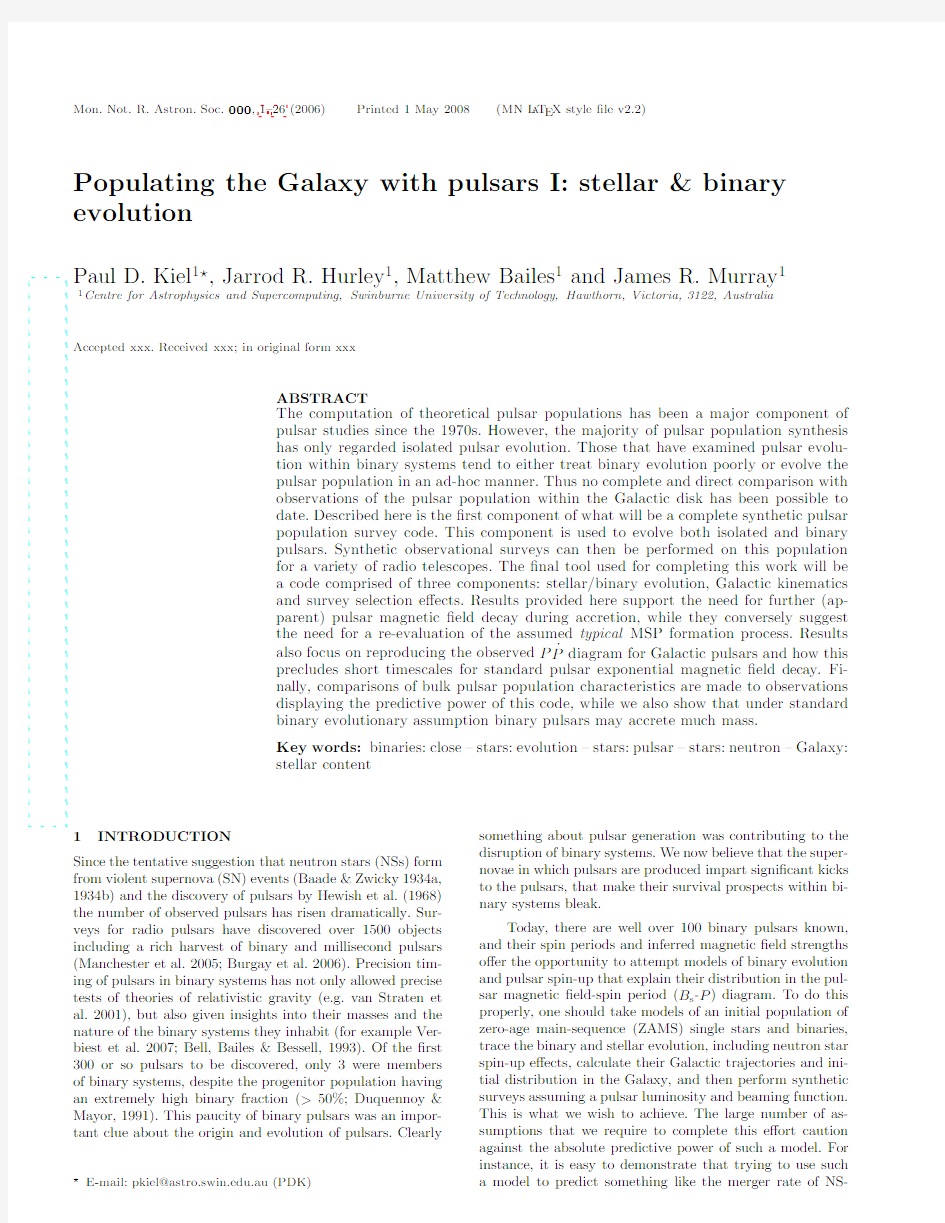
As alluded to above,observations of pulsars take the form of spin measurements–both the spin period P and spin period derivative˙P–in which the surface magnetic ?eld B s and characteristic age of the pulsars are inferred (details are discussed when we introduce our model of pul-sar evolution).It is instructive to plot˙P vs P(hereafter P˙P)and B s vs P diagrams and any theoretical model must be
able to reproduce these if it is to be successful.In Fig-ure1we show the B s vs P diagram of~1400pulsars taken from the ATNF Pulsar Catalogue1(Manchester et al.2005). We see three distinct regions of the parameter space being populated.A large island of relatively slow spinning pul-sars with high surface magnetic?elds(and thus high˙P s)is joined via a thin bridge of pulsars to another,smaller,island of relatively rapid rotators with low magnetic?elds.
The present theoretical explanation for the distinct groups of observed pulsars is rotating magnetic neutron stars that are either isolated or reside in a binary system(see Wheeler1966;Pacini1967;Gold,1968;Ostriker&Gunn 1969;Gunn&Ostriker1970;Goldreich&Julian1969,van den Heuvel1984,Colpi et al.2001;Bhattacharya2002; Harding&Lai2006).It is those NSs that evolve within a binary system that may attain the low surface magnetic ?elds and low rotational periods,i.e.rapid rotators,as men-tioned above.The double pulsar binary J0737-3039A&B (Burgay et al.2003;Lorimer2004;Lyne et al.2004;Dewi& van den Heuvel2004)shows the distinction between rapid rotators and slow rotators clearly.Here we have a binary system consisting of a millisecond pulsar(MSP:P=22.7 ms and B s=7×10⁹G)and its‘standard’pulsar com-panion(P=2.77s and B s=6×10¹²G).Although it seems likely that it is the process of accretion onto the NS that induces NS magnetic?eld decay(or apparent mag-netic?eld decay)this evolutionary phase is still highly con-tentious and theories abound on how the decay may occur. One such theoretical argument is of accretion-induced?eld decay via ohmic dissipation of the accreting NSs crustal cur-rents.This is due to the heating of the crust which in turn increases the resistance in the crust(Konar&Bhattacharya 1997,1999a,1999b;Geppert&Urpin1994;Urpin&Gep-pert1995;Romani1990;Urpin,Geppert&Konenkov1997). An alternative explanation of accretion-induced?eld decay 1http://www.atnf.csiro.au/research/pulsar/psrcat/Figure 1.Magnetic?eld vs spin period of observed pulsars within the Galaxy(stars,including some within globular clus-ters).The observations are overlaid with a cartoon depiction of the reason for the particulars of the pulsar parameter space distribution.The area covered by vertical bars primarily arises from the canonical pulsar birth properties and spin-down due to magneto-rotational energy losses.The horizontal barred re-gions are formed for the most part by deviation of pulsar birth properties from the average values from whence pulsar spin-down evolution commences.Forward leaning horizontal bars depict the region in which a luminosity law or loss of obliquity of beam direc-tion(or a combination of these)induces a decrease of numbers in the observed population.The?nal observed pulsar region arises from binary evolution,although a number of these systems are isolated it is possible they were formed in binaries which disrupted due to the explosion or ablation of the secondary star. consists of screening or burying the magnetic?eld with the accreted material(Lovelace,Romanova&Bisnovatyi-Kogan 2005;Konar&Choudhuri2004;Choudhuri&Konar2002; Cumming,Zweibel&Bildsten2001;Melatos&Phinney 2001;Bisnovatyi-Kogan&Komberg1974;Taam&van den Heuvel1986).While yet another argument considers vortex-?uxoid(neutron-proton)interactions.Here the neutron vor-tices latch on and then drag the proton vortices(which bear the magnetic?eld)radially,the radial direction is induced by either spin-up(inwards)or spin-down(outwards)of the NS(Jahan-Miri2000;Muslimov&Tsygan1985;Ruderman 1991a,b&c).
Below is a general overview of pulsar evolutionary paths.A greater level of detail is given within the very in-formative reviews presented by Colpi et al.(2001),Bhat-tacharya(2002),Choudhuri&Konar(2004),Payne& Melatos(2004),Harding&Lai(2006)and references therein.There are a number of possible binary and stellar evolutionary paths one can conceive that allow the forma-tion of a pulsar.If the end product is an isolated‘standard’pulsar,the star may have always been isolated and evolved from a massive enough progenitor star(mass greater than ~10M⊙)with no evolutionary perturbations from outside in?uences.However,it may have been that the progenitor
Pulsar Population3
pulsar was bound in an orbit and depending on the orbital parameters when the NS formed,mass loss and the veloc-ity kick during the asymmetric SN event(Shklovskii1970) could contrive to disrupt the binary,allowing us to observe a solitary pulsar.Alternatively,if the secondary star was also massive(but originally the less massive of the two stars) disruption may occur in a second SN event.The creation of a millisecond(re-cycled;Alpar et al.1982)pulsar requires the accretion of material onto the surface of the NS at some point during its lifetime.For this to occur the primary star is ?rst required to form a NS and the binary must survive the associated SN event.Then,some time later,the secondary star evolves to over?ow its Roche-lobe and initiate a steady mass transfer phase.Any accretion of the donated material onto the NS will increase its spin angular momentum,thus spinning up the pulsar,potentially to a millisecond spin pe-riod.The companion of the resultant MSP will typically be a low-mass main sequence star,a white dwarf(WD:a MSP-WD binary)or another pulsar.Formation of a double pulsar binary is problematic because if more than half of the sys-tems mass is lost in the second SN event the binary will be disrupted.This is unless a kick is directed toward the vicin-ity of the companion MSP with just the right magnitude to overcome the energy change owing to mass loss but not too strong as to disrupt the binary.If instead the binary is disrupted by the SN then there would be both a solitary ‘standard’pulsar and a single MSP.One other suggested method for producing a single millisecond pulsar is for the donor star to be evaporated or ablated by the extremely ac-tive pulsar radiation(which may be modelled in the form of a wind).The pulsar is then said to be a black widow pulsar (van Paradijs et al.1988).
As mentioned above,the theories of pulsar evolution can be tested in a statistical manner by comparing observations to population synthesis results.This theoretical approach has been adopted previously for pulsars and other stellar systems(some examples are:Dewey&Cordes1987;Bailes 1989;Rathnasree1993;Possenti et al.1998;Portegies Zwart &Yungelson1998;Possenti et al.1999;Willems&Kolb 2002;O’Shaughnessy et al.2005;Kiel&Hurley2006;Dai, Liu&Li2006;Story,Gonthier&Harding2007and numer-ous works based on StarTrack,presented in Belczynski et al.2008).The level of detail in the population synthesis cal-culations varies,along with the methodologies the authors implemented.For example,Bailes(1989)considered pulsar selection e?ects in some detail,however,only roughly con-sidered binary evolutionary phases and the method in which this a?ects pulsar evolution.Willems&Kolb(2002)consid-ered NS populations and how these a?ect the resultant NS populations,however,they were not able to directly com-pare with observations as no selection e?ects were modelled. In a slightly di?erent approach(empirically based)Kim, Kalogera&Lorimer(2003)estimated the merger rate(via gravitational waves)of double NS(DNS)binaries within the Galaxy by selecting the physical observable DNS pulsar properties from appropriate distribution functions for many pulsars and weighting these against the observed Galactic disk DNS pulsars PSR B1913+16and PSR B1534+12.Tak-ing into account selection e?ects of the pulsar population for large scale surveys and producing many pulsar models they were able to give con?dence levels for their merger rate esti-mates.In comparison,we will select the initial
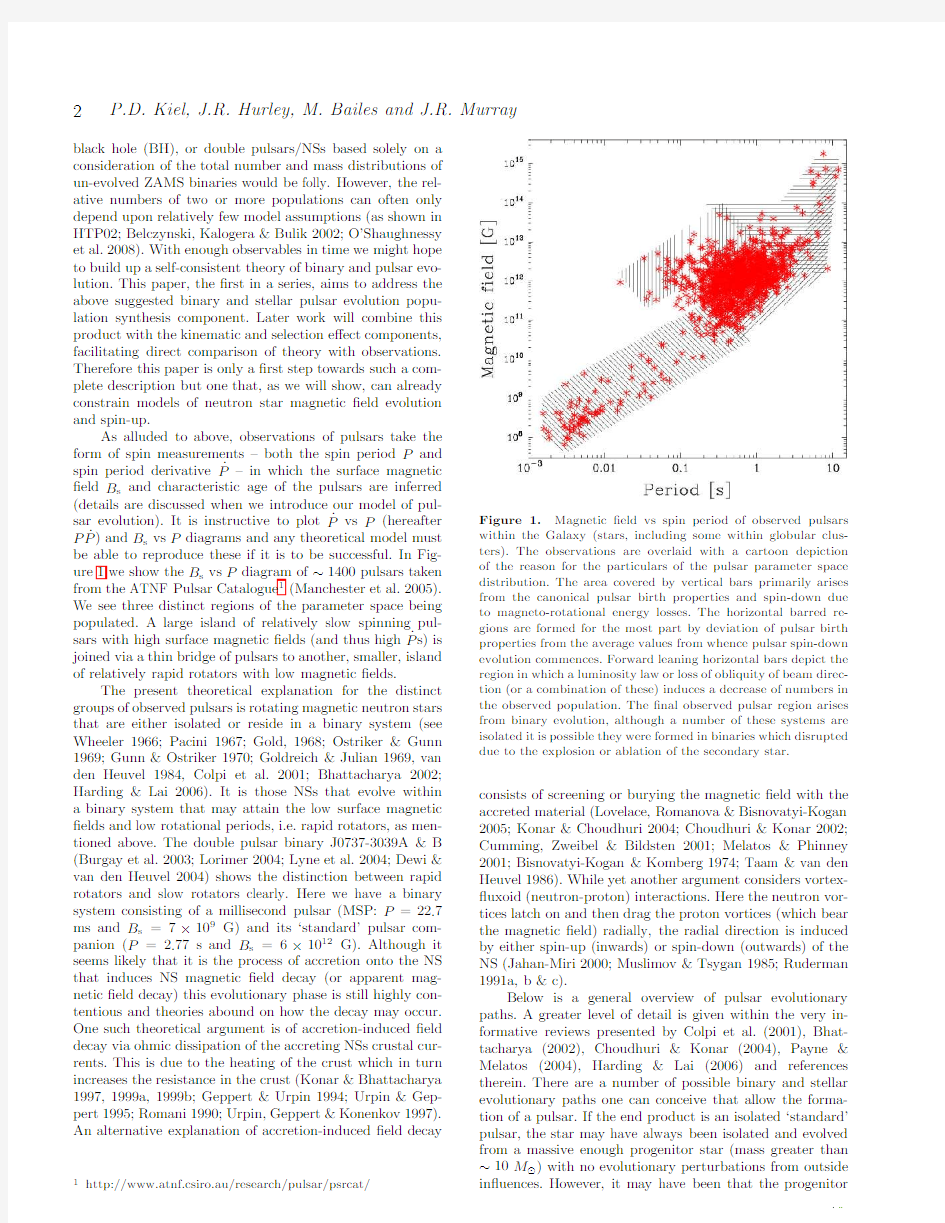
evolutionary Figure2.Flow chart of our synthetic pulsar population survey process.The work presented here focuses on the?rst module, binpop(see text for details).
parameters from distribution functions and evolve all stars forward in time from stellar birth on the ZAMS through un-til the current time.This gives us the ability to constrain many stellar and binary evolutionary features while lending us the?exibility to,for example,compare di?erent popula-tions of stars with each other and observations.In this way we can aim to further constrain uncertain parameter values. However,even at this early stage we must place a strong word of caution regarding the issue of parameter variation –strong degeneracies can apply amongst parameters(e.g. O’Shaughnessy et al.2005),where a succession of parameter changes can mask the e?ect of another,so extensive mod-elling is required before de?nite conclusions can be made.
Our goal is to create a generic code for producing syn-thetic Galactic populations.This will comprise three mod-ules:binpop,binkin and binsfx(see the?ow chart in Fig-ure2for a representation of how these?t together).The ?rst module,binpop,covers the stellar and binary evolu-tion aspects and as such is a traditional population synthesis code in its own right.The second module,binkin,follows the positions of both binary systems and single stars within the Galactic gravitational potential.The third module im-poses selection e?ects on the simulations,thus giving simu-lated data that can compare directly to observations.This last consideration is in some regards the most important as without detailed modelling of selection e?ects any compar-ison of population synthesis simulations to observations is crude(Kalogera&Webbink1998).This paper focuses on a description of the binpop module and,in particular,the pulsar population that it produces.We consider in depth modelling of pulsar evolution in terms of the spin period and the magnetic?eld coupled with mass accretion.Sim-ulating these processes will help in constraining the stellar birth properties of NSs and also lead to a greater under-standing of aspects of NS evolution such as the formation event itself–the supernova.It will also allow predictions of the composition of the Galactic pulsar population.Follow-up work will discus binkin with a focus on the kinematic evolution of the pulsar distribution within the Galaxy,and SN veolicty kicks–and binsfx.
This paper is organised as follows.Section2gives an overview of the rapid binary evolution population synthesis code used in this research.This is followed in Section3by a detailed description of the pulsar modelling techniques that have been added to this code to create binpop.Section4 gives examples of the pulsar evolutionary pathways that can be followed with binpop and how these can be a?ected by
4P.D.Kiel,J.R.Hurley,M.Bailes and J.R.Murray
choices in the algorithm.Population synthesis results in the form of P˙P comparisons are given in Section5followed by a discussion in Section6.In particular we wish to draw the readers attention to the results shown in Section5.8.5which extend beyond the basic P˙P description.
2RAPID BINARY EVOLUTION&
POPULATION SYNTHESIS
The research presented here makes use of the?rst mod-ule of our synthetic Galactic population code.This is called binpop and wraps the Hurley,Tout&Pols(2002:HTP02) binary stellar evolution(bse)code2(with updates as described in Section3)within a population synthesis pack-age.
The bse algorithm is described in detail by HTP02and an overview is given in Kiel&Hurley(2006).The aim of bse is to allow rapid and robust,yet relatively detailed, binary evolution based on the most up-to-date prescrip-tions/theories for the various physical processes and scenar-ios that are involved.In its most basic form the bse algo-rithm can be thought of as evolving two stars forward in time–according to the single star evolution(sse)pre-scription described in Hurley,Pols&Tout(2000)–while up-dating the orbital parameters.After each time-step the algo-rithm checks whether either star has over-?owed its Roche-lobe and depending on the result the system is evolved ac-cordingly,i.e.as a detached,semi-detached,or contact bi-nary.During these phases the total angular momentum of the system is conserved while orbital and spin changes ow-ing to tides,mass/radius variations,magnetic braking and gravitational radiation are modelled.
Within bse an e?ort is made to model all relevant stellar and binary evolutionary processes,such as mass transfer and common-envelope(CE)evolution.Invariably this involves making assumptions about how best to deal with elements of the evolution that are uncertain.An example that is rele-vant to pulsar evolution is the choices made for the nature of the star produced as a result of the coalescence of two stars, where at least one NS is involved.If the merger involves a NS and a non-degenerate star then a Thorne-˙Zytkow object (T˙ZO:Thorne&˙Zytkow1977)is created.Detailed mod-elling of these objects must deal with neutrino physics and processes such as hypercritical accretion and currently the ?nal outcome is uncertain(Fryer,Benz&Herant1996;Pod-siadlowski1996).Possibilities include rapid ejection of the envelope(the non-degenerate star)to leave a single NS that has not accreted any mass or collapse of the merged object to a BH.In bse the former is currently invoked–an unsta-ble T˙ZO.On the other hand,the coalescence of a NS with a degenerate companion is assumed to produce a NS with the combined mass of the two stars,unless the companion is a BH in which case the NS is absorbed into the BH.For steady transfer of material onto a NS–in a wind or via Roche-lobe over?ow(RLOF)–it is assumed in bse that the NS can accrete the material up to the Eddington limit(Cameron& Mock1967).However,there is some uncertainty as to what 2See also https://www.doczj.com/doc/aa14730271.html,.au/~jhurley/and relevant links.extent this limit applies as there may be cases where energy generated in excess of the limit can be removed from the sys-tem(e.g.Beloborodov1998).For this reason the Eddington limit is included as an option in bse(HTP02).Another area of uncertainty is what happens to a massive oxygen-neon-magnesium WD when it accretes enough material to reach the Chandrasekhar limit–does it explode as a mass-less su-pernova or form a NS?Currently bse follows the models of Nomoto&Kondo(1991)which suggest that electron cap-ture on Mg24nuclei leads to an accretion-induced collapse (AIC)and a NS remnant(Michel1987).In the formation of a NS via the AIC method bse assumes that no velocity kick is imparted onto the NS while some other population synthesis works have assumed a small but non-zero velocity kick for these NSs(Ivanova et al.2007;Ferrario&Wickramasinghe 2007).These examples illustrate some of the decision making involved with creating a prescription-based evolution algo-rithm and the interested reader is directed to HTP02for a full description as well as a list of options included within the bse code.
Subsequent to HTP02the following changes have been made to the bse algorithm:
?an option to calculate supernova remnant masses us-ing the prescription given in Belczynski,Kalogera&Bulik (2002)which accounts for the possibility of the fall-back of material during core-collapse supernovae(this is now the preferred option in bse);
?an algorithm to compute the stellar envelope structure parameter,λ,(required in CE calculations)from the results of detailed models(Pols,in preparation)–previously this was set to a constant whereas models show that it varies with mass and evolution age(Dewi&Tauris2001;Podsiadlowski et al.2003);
?the addition of equations to detect,and account for,the existence of an accretion disk during mass transfer on to a compact object(following Ulrich&Burger1976);and,?an option to reduce the strength of winds from helium stars.
These changes are documented in greater detail by Kiel& Hurley(2006).Further additions to the bse algorithm relat-ing to pulsar evolution will be described in the next section.
There are also a number of areas where the bse al-gorithm could be improved in the future.The integration scheme used for the di?erential equations in bse(and for the equations introduced here)employs a simple Euler method (Press et al.1992)with the time-step depending primarily on the nuclear evolution of the stars.It has been suggested that this will lead to inaccurate results for the orbital evo-lution,in particular when integrating the tidal equations (Belczynski et al.2008),and an implementation of a higher-order scheme will be a priority for the next revision of the bse code.It will also be desirable to include a RLOF treat-ment for eccentric binaries and the addition of an option for tidally-enhanced mass-loss from giant stars close to RLOF (along the lines of Bonaˇc i′c Marinovi′c,Glebbeek&Pols 2008).Another area of uncertainty is the strength of stellar winds from massive stars(Belczynski et al.2008).This is a feature which can be varied within bse but we do not utilise it or examine its e?ect on compact object formation in this work.
Re?ecting the variety of processes involved in binary
Pulsar Population5
evolution,and the uncertain nature of many of these,there are inevitably a substantial number of free parameters asso-ciated with a binary evolution code.Unless otherwise speci-?ed we assume the standard choices for the bse free param-eters as listed in Table3of HTP02.This includes setting αCE=3for the CE e?ciency parameter.In addition we use the variableλfor CE evolution and the remnant mass rela-tion of Belczynski et al.(2002),as described above.We also useμnHe=0.5in the expression for the helium star wind strength(see Kiel&Hurley2006for details)and we impose the Eddington limit for accretion onto remnants.Where ap-plicable(Sections4and5)we will take care to note our choices for any bse parameters that we vary.
Our aim is to produce a Galactic population of pul-sars.We do this using the statistical approach of population synthesis.The?rst step is to produce realistic initial popu-lations of single and binary stars.For each initial binary the primary mass,secondary mass and orbital separation are drawn at random from distributions based on observations (see Section5.1for details).For single stars only the stellar mass is required for each star.We then set a random birth age for each binary(or star)and follow the evolution to a set observational time.By selecting those systems that evolve to become pulsars we can produce a P vs˙P diagram for the Galactic pulsar population–assuming(at least initially) that all generated pulsars are observable.This is repeated for a variety of models and comparisons made to observa-tions.This is the method we use here.However,it is possible to determine the initial parameters from a set grid and then convolve the results with the above mentioned initial distri-bution functions to determine if the binary contributes to the Galactic population.For more information on the grid method see Kiel&Hurley(2006).
3MODELLING A PULSAR
We now describe our methods for evolving pulsars–both isolated and within a binary system.This requires a num-ber of additions to the bse algorithm.We point out here that although most important phases of stellar and binary evolution are modelled we still draw the initial pulsar evolu-tionary parameters–spin period and magnetic?eld–from distributions.This is the method employed in all previous pulsar population synthesis simulations.The need for this arises because there is no complete theoretical method for modelling the SN event(Janka et al.2006),and thus no strong link between the pre-SN star and post-SN star.As-pects such as the initial NS mass,however,are better deter-mined.Also,kick velocities imparted to NSs at birth are gen-erally selected from distributions that match observations of NS space velocities.We investigate the initial NS spin period and magnetic?eld distributions and extend previous studies by linking these to this kick velocity(see Sections3.4and 5.5).We also note that although some previous pulsar popu-lation synthesis studies take into account selection e?ects to allow direct comparison with observations we do not do this here in any detail.As a?rst step we do consider beaming e?ects but mainly we leave this for future work.Our wish at this stage is to test that our evolution algorithm can pop-ulate the required regions of the observed parameter space. Considering direct number and birth rate comparisons with observations will follow when the full three module code is complete.
3.1Previous e?orts
There have been many attempts at modelling NS evolu-tion.Some,as given in the introduction,try to generalise or parametrise the evolution to allow rapid computation for statistical considerations.Another method,however,is to perform detailed modelling of a single NS.Debate on NS evolution has concentrated mainly on the structure of NSs and the evolution of the magnetic?eld.Most statisti-cal studies have considered only those NSs that are isolated pulsars and here concern is,generally,on the magnetic?eld decay timescale or space velocity and magnetic?eld correla-tion.The semi-analytical studies of Gunn&Ostriker(1970), Phinney&Blandford(1981),Vivekanand&Narayan(1981) and Lyne,Manchester&Taylor(1985)found a magnetic ?eld decay timescale of order a few million years.In compar-ison,studies by Taylor&Manchester(1977),van den Heuvel (1984)and Stollman(1987)found the decay timescale to be>100Myr.More recently population studies of pul-sars have tended towards a greater level of detail in the treatment of pulsar evolution and modelling of selection ef-fects.Again,di?ering studies?nd a variation of magnetic ?eld decay time-scales.Those such as Bailes(1989),Rath-nasree(1993);Bhattacharya et al.(1992),Hartman et al. (1997),Lorimer et al.(1993),Lorimer,Bailes&Harrison (1997),Regimbau&de Freibas Pacheco(2000),Regimbau &de Freibas Pacheco(2001),Dewi,Podsiadlowski&Pols (2005)and Faucher-Giguere&Kaspi(2006)conclude that ?eld decay occurs on timescales comparable to the age of old pulsars.While Gonthier et al.(2002)and Gonthier,Van Guilder&Harding(2004)suggest NSs evolve with shorter decay time-scales(~few Myr).However,Faucher-Giguere &Kaspi(2006)suggest this later result is an artifact of the pulsar radio luminosity law assumed by Gonthier et.al. (2002)and Gonthier,Van Guilder&Harding(2004).The ?eld decay time-scale is a parameter within our models that is allowed to vary.As we will here,Dewey&Cordes(1987), Bailes(1989),Rathnasree(1993),Dewi,Podsiadlowski& Pols(2005)and Dai,Liu&Li(2006)take into consideration pulsars that may evolve within binary systems and follow the orbital properties along with the pulsar spin and magnetic ?eld.Previously either the treatment of binary evolution or pulsar evolution has been limited,although the work of Dai, Liu&Li(2006)utilises the bse and a limited form of pulsar physics.No published work to date has fully considered the e?ect of magnetic?eld decay within both single and binary pulsar evolution in such detail as presented here.
3.2Single or wide binary pulsar evolution
We?rst consider the evolution of a NS that does not accrete any material,either an isolated NS or one in a wide enough orbit to allow single star-like evolution.Although,in the latter case we note that aspects of binary evolution such as tidal interaction are followed in step with the pulsar spin evolution.We evolve a solitary pulsar by assuming a pulsar magnetic-braking model of the form,
6P.D.Kiel,J.R.Hurley,M.Bailes and J.R.Murray
˙P=K B2s
τB ,(2) where B s0is the initial NS surface magnetic?eld,T is the age of the pulsar,τB is the magnetic?eld decay time-scale and t acc is the time the pulsar has spent accreting matter via RLOF.Allowing the magnetic?eld to decay is inspired by observations,where older isolated pulsars are shown to have lower magnetic?elds than younger pulsars and is now a standard evolutionary model within the literature(Gunn &Ostriker1969;Stollmen1987).This apparent magnetic ?eld decay is still observed even when detailed modelling of selection e?ects are taken into account(Faucher-Giguere& Kaspi2006),though as mentioned above the timescale varies due to assumptions used within the modelling.To integrate these equations into the bse we must follow the angular momentum of the NS using the magnetic-braking model of Equation1.Di?erentiating the angular velocity with time and applying the chain rule we have the angular velocity time derivative,
˙?=??
P2
B2s(4) =?
K
5
MR2˙?,(7) which is the angular momentum equation for a solid spher-ical rotator with radius R,mass M and angular velocity?. This is then removed from the total NS angular momentum, the system is updated(this includes the NS spin-down being transfered to the orbital angular momentum via tides)and we step forward in time.
In the work presented here we are evolving the surface magnetic?eld,B s of the NS.Strictly speaking if we were to compare our theoretically calculated magnetic?eld to ob-servations we should use the magnetic?eld strength at the light cylinder radius–that is the radius at which if the mag-netic?eld is considered a solid rotator it is rotating at the speed of light.When observations of the spin period and spin period derivative are made it is the magnetic?eld at this ra-dius that is being sampled.When we calculate the period derivative this assumed change of magnetic?eld is taken into account and as such we have two reasons for comparing our theoretical models to observations in the period-period derivative parameter space.Firstly,it is˙P that is actually being measured observationally and secondly the˙P calcula-tion naturally takes into account the light cylinder magnetic ?eld(as it makes use of the pulsar magnetic moment).
3.3Pulsar evolution during accretion
Allowing the decay of a NSs magnetic?eld during an ac-cretion event is believed to be the cause of the observed pulsar P˙P distribution(see Section1).Until now this has not been tested with any detailed modelling of binary,stel-lar and pulsar evolutionary physics.During any accretion phase angular momentum is transfered to the accreting ob-ject and it is spun-up.To follow this evolution we use the standard equations describing the system angular momen-tum as given in HTP02.While steady mass transfer occurs we do not allow any decrease in the NS rotational veloc-ity due to the magnetic-braking process described by Equa-tion6.Instead the NS angular momentum increases while the magnetic?eld decays exponentially with the amount of mass accreted,
B s=B s0exp ?k?M
1+?M
Pulsar Population7
the NS but instead of following the magnetic?eld lines to the surface the material is ejected from the system by the rapidly rotating magnetic?eld lines.The magnetic?eld acts as a propeller,changing rotational energy of the NS into ki-netic energy for the now outgoing matter.This phase has a noticeable e?ect on the NS.Due to the loss of rotational energy by the NS it spins down.This is therefore an im-portant evolutionary phase to consider during accretion and we have implemented a method for modelling it within bse. We follow Jahan-Miri&Bhattacharya(1994)who allow the di?erence between the Keplerian angular velocity,?K,at the pulsar magnetic radius R M and the co-rotation angular velocity,??,(V di?=?K(R M)???)to decide whether the accretion phase spins the NS up or down.The magnetic ra-dius is assumed to be half the Alfven radius,R m,the radius at which the magnetic pressure balances the ram-pressure, B2s R6
4πR5/2
m
.(10) This gives
R m=3.4×10?4R⊙ B2s R6
3
Ξwind?MR22?2,(13) where J wind is the angular momentum transferred in the wind,?M is the accreted mass,R2is the companion stel-lar radius and?2is the companion star angular velocity. Basing the variability ofΞwind on the assumption that the NS magnetic?eld plays an integral part when NS angular momentum accretion occurs,we allowΞwind to vary as,Ξwind=MIN 1,0.01 2×10¹¹/B s +0.01 .(14) By assuming the above form ofΞwind we allow larger mag-netic?elds to dominate the?ow of angular momentum, while the simplicity depicts our lack of knowledge of the physical processes in such an evolutionary phase.An exam-ple of the uncertainty is shown in the work of Ru?ert(1999) who estimates an angular momentum accretion e?ciency between0.01and0.7(hence our lower limit forΞwind).
3.4Initial pulsar parameter selection
As mentioned earlier previous pulsar population synthesis work begin by selecting the initial period,magnetic?eld, mass,etc,of the pulsar from distributions,ignoring any ear-lier evolutionary stages the star may have passed through.If the distributions for each parameter are realistic this method is considered robust to?rst order.This is the method fol-lowed here for the initial spin period of the pulsar,P0,and the initial surface magnetic?eld,B s0.We select from?at distributions between P0min and P0max for the initial spin pe-riod and between B s0min and B s0max for the initial magnetic ?eld.Typical values for these parameters are P0min=0.01s, P0max=0.1s,B s0min=1012G and B s0max=3×10¹³G, although these can vary(see Table1).
In actual fact the exact initial pulsar spin period and magnetic?eld distributions are unknown.However,Spruit &Phinney(1998)have previously suggested that there is a connection between the three pulsar birth characteristics: imparted velocity,spin period and magnetic?eld strength.
A parameter linked to the SN event and one in which we claim to have some form of observational contraint is V kick. The velocity kick is randomly selected from a Maxwellian distribution with a dispersion of Vσ(as in HTP02and Kiel &Hurley2006).With this in mind we trial a method in which the initial pulsar birth parameters P0and
B s0are linked to V kick.In this‘SN-link’method we have,
P0=P0min+P0av(V kick/Vσ)n p,(15) and
B s0=B s0min+B s0av(V kick/Vσ)n b,(16) where P0av is the average initial period and B s0av is the av-erage initial magnetic?eld.The exponents n p and n b allow us to parameterise the e?ect the SN event has on the initial pulsar period and magnetic?eld but we take both equal to one throughout this work.An assumption here is that a more energetic explosion would be able to impart a greater initial angular velocity onto the proto-NS than a lesser explosion, which may in turn introduce a more e?ective dynamo action increasing the initial magnetic?eld strength.
We note here that due to the lack of a complete under-standing of SNe,we are at present not attempting to?nd the true pulsar initial period and magnetic?eld distributions but trying to depict how modifying the initial pulsar birth region in the P˙P distribution a?ects the?nal pulsar P˙P distri-bution.Previous population synthesis models have di?ered on their preferred initial parameter distributions(compare Faucher-Giguere&Kaspi2006and Gonthier,Van Guilder &Harding2004;Story,Gonthier&Harding2007),however, any complete pulsar population synthesis must be able to re-produce the observed pulsars associated with SN remnants.
8P.D.Kiel,J.R.Hurley,M.Bailes and J.R.Murray
3.5Electron capture supernova
An important phase in NS evolution which we have touched
on brie?y already is the birth of NSs in SN events.Previ-
ous numerical models of SNe suggested that convection may drive the formation of assymetries in SNe(Herant,Benz
&Colgate1992;Herant et al.1994).More recently there
have been exciting developments in this area driven by the successful modelling of SN explosions in multi-dimensional
(spatially)hydrodynamic simulations(Mezzacappa et al.
2007;Marek&Janka2007;Fryer&Young2007).These models show high levels of convection due to the stationary
accretion shock instability(found numerically by Blondin&
Mezzacappa2003).This instability leads to an asymmetry in the explosion event and provides a mechanism for deliver-
ing large SN velocity kicks.Observationally,proper motion
studies of pulsars have detected large isolated pulsar space velocities of order1000km/s(e.g.Lyne&Lorimer1994).
Furthermore,mean pulsar space velocities appear to be in
excess of the mean for normal?eld stars(e.g.Hobbs et al. 2005).These results show the necessity of imparting veloc-
ity kicks to NSs.As such most previous population synthesis
works have assumed a Maxwellian SN velocity kick distri-
bution with Vσ~200?500km/s(see above in Section3.4).
Of late however,there has been a body of evidence that
some NSs must have received small velocity kicks,of order 50km/s(Pfahl et al.2002;Podsiadlowski et al.2004).Ob-
servationally Pfahl et al.(2002)found a new type of high-
mass X-ray binary which exhibited low eccentricities and
wide orbits,suggesting a low velocity kick imparted during the SN event.This is backed up by evidence of the relatively
large amount of NSs within globular clusters compared to
the estimated number if one considers they receive an av-erage velocity kick of Vσ>200km/s(Pfahl,Rappaport
&Podsiadlowski2002;and more recently in the theoreti-
cal studies of Kuranov&Postnov2006and Ivanova et al. 2007).The type of SN explosion that theoretically causes
small velocity kicks,and is in vogue at present,is the elec-
tron capture(EC)method.Basically this is the capture of electrons in the stellar core by the nuclei24Mg,24Na and 20Ne(Miyaji et al.1980,see their Figure8and Table1). This results in a depletion of electron pressure in the core, facilitating the core collapse to nuclear densities if the?nal
core mass is within the mass range of1.4to2.5M⊙(Nomoto
1984;1987).The bounce of material due to the halt of the collapse by the strong force thus drives the traditional SN event.Taking into account both single star evolution(Poe-larends et al.2007)and binary evolution(Podsiadlowski et al.2004)suggests that the initial mass range of stars that may explode via the EC SN mechanism resides somewhere within6?12M⊙,with some dependence on metallicity and assumptions made in stellar modelling.Early work on the EC SN explosions suggested that it is a prompt event, in which any asymmetries would not have time to occur. Thus allowing the nascent NS a small SN kick velocity.This is in contrast to SN explosions from more massive initial mass stars(>12M⊙)which produce rather slow explo-sions(many hundreds of ms;Marek&Janka2007).We note that the latest oxygen-neon-magnesium SN explosions(ini-tial stellar mass range of8?12M⊙)by Kitaura,Janka& Hillebrandt(2006)show that the EC SN is not so prompt as previously thought(few hundred ms)and also energy yields are a factor of10less.However,these authors still?nd low recoil velocities for the nascent NS,again because hydrody-namic instabilities are unlikely to form.
As detailed in Ivanova et al.(2007)there are a number of stellar and binary evolutionary pathways which may lead to EC SN.Although EC SN may occur from processes of sin-gle star evolution we concentrate here on a relatively newly recognised binary evolution example(Podsiadlowski et al. 2004).A primary star with a zero-age-MS mass between ~8?12M⊙that lives in the appropriate binary system may experience a mass transfer phase in which its convec-tive envelope is stripped from it before the second dredge-up phase on the asymptotic giant branch.This lack of second dredge-up leaves behind a more massive helium core than would otherwise have remained if the hydrogen-rich enve-lope had not been stripped o?.Yet it is a less massive core than is left behind for stars>12M⊙(see Podsiadlowski et al.2004,Figure1).Depending upon the rate of mass loss via a wind the helium core may then evolve through the relevant phases to explode as an EC SN(Podsiadlowski et al.2004).The ability for a binary system to produce a he-lium star with a mass within the assumed range of1.4to 2.5M⊙as given above is much greater than for a single star (Podsiadlowski et al.2004).
The possibility of EC SNe is included as an option in bse for the following cases:
?a giant star with a degenerate oxygen-neon-magnesium core that reaches the Chandrasekhar mass–for the stellar evolution models used in bse this coresponds to an initial mass range of~6?8M⊙(for solar metalicity:HTP02);
?a helium star with a mass between1.4M⊙?2.5M⊙(as set by Podsiadlowski et al.2004based on the work of Nomoto1984;1987).
When a NS forms in these cases we use an electron capture kick distribution with Vσ=20km/s(see NS kick distribu-tion of Kiel&Hurley2006).
3.6NS magnetic?eld lower limit
Most detailed magnetic?eld decay models show a‘bottom’or lower limit value of the magnetic?eld in which no further decay is possible.Here,this lower limit is a model parameter, B bot,and,as given in Zhang&Kojima(2006),should be of order107?108G.We use5×107G throughout this work.
3.7Radio emission loss:The death line Generally,it is believed electron-positron pairs are the par-ticles that,when accelerated within the magnetic?eld of a NS,produce the observed radio emission.These pairs are assumed to form in the polar cap(PC)region of the NS (PC model:Arons&Scharlemann1979;Harding&Mus-limov1998)or in the outer NS magnetosphere beyond the polar caps(as in the outer gap model:Chen&Ruderman 1993).Depending upon the chosen model it is possible to predict when or under what circumstances a NS will turn o?its beam mechanism and thus stop being observable as a pulsar.These predictions form a region in the P˙P parameter space where the NS is not able to sustain pair production. The edge of this region is commonly referred to as the pul-sar death line.Until recently e?orts within pulsar population
Pulsar Population9 synthesis calculations for simulating the death-line have only
considered isolated pulsars.Such models have been based on
the work by Bhattacharya et al.(1992)who,following Ru-
derman&Sutherland(1975),give the condition,
B s
8
log(P)?
7
2
log(I)+
19
2
log(P)?2log ˉf min prim (22)
?
3
7 1?2.42×10?6M R2
?1MR2(24)
and
R=2.126×10?5M?1/3.(25)
Here,I is taken from Tolman(1939)and as shown in Figure6
of Lattimer&Prakash(2001)this equation is a good?t
to detailed models of NSs for di?ering equation of states
down to M
10P.D.Kiel,J.R.Hurley,M.Bailes and J.R.
Murray
Figure3.The evolution of pulsar particulars,P,B s and˙P for di?ering initial parameter P and B s values.There are two isolated pulsar evolutionary pathways depicted here,these are the dotted paths.Two binary pulsar evolutionary paths are also shown(pluses and circles).See text for further details.
spin period,magnetic?eld and period derivative are shown in Figures3a),b)and c)respectively(the lower dotted curves in each plot).The evolution in the P˙P diagram is shown in Figure3d).
After10Gyr the stellar spin period,magnetic?eld and period derivative are‘observed’as,0.76s,3.7×108G and 2.04×10?22s/s respectively.No pulsar has ever been ob-served with such parameters,so it is safe to assume that this NS,after10Gyr,would be beyond the pulsar death line.In fact,if we assume a death line of the form given by Equation17then the pulsar would die after a system time of4555Myr.This is the case if we assumeτB=1000 Myr.However,if we assume instead that the magnetic?eld decays on a much faster time-scale,say,τB=5Myr,then the NS parameters evolve to a somewhat di?erent con?g-uration.In this case the NS ends with P=6.9×10?2s, B s=5×10⁷G and˙P=3.6×10?23s/s.Here the NS mag-netic?eld reaches the lower limit of5×107G in just over 600Myr which is about the same time that the pulsar would cross the death line.If we assume the star has a metallicity of0.001or0.0001then a BH is born directly.This is be-cause the boundary between NS and BH formation(which is governed by the asymptotic giant branch core mass which collapses to a3M⊙remnant)varies slightly with metallic-ity.In terms of initial stellar mass this is about21M⊙for
Pulsar Population
11 Figure4.The evolution of pulsar particulars,P,B s and˙P for di?ering evolutionary assumptions,τB(plus),k(circles)and propeller (cross).
solar metallicity whereas for a Z=0.0001population it is 19M⊙.
4.2A binary MSP
We now consider the same NS/pulsar as before but place it within a binary system.The initially20M⊙primary star(NS progenitor)has a5.5M⊙companion in a circu-lar P orb=32day(a=125R⊙)orbit.Initially the stars are assumed to reside on the ZAMS.Due to the greater mass of the primary star it evolves more quickly than its secondary companion,leaving the MS at the same time as its isolated counterpart of the previous example(as compared to the secondary,who leaves the MS after540Myr).The primary evolved to?ll its Roche-lobe at a system time of8.8Myr. At this point it is in the HG phase of evolution and has lost ~1M⊙in a stellar wind–the secondary accreted0.285M⊙of this and was spun up accordingly.At the onset of RLOF mass transfer occured on a dynamical timescale and lead to formation of a common-envelope.During the common en-velope phase the MS secondary and the primary core spiral in toward each other with frictional heating expelling the CE.This phase is halted when the entire envelope is re-moved(~14M⊙)and the two stars are just8R⊙apart.At this stage the MS secondary star is extremely close to over-?owing its Roche-lobe radius,however,the primary star–now being a naked helium star–continues to release mass in the form of a wind(which we assume has the form given in
12P.D.Kiel,J.R.Hurley,M.Bailes and J.R.Murray
Kiel&Hurley2006)and due to conservation of angular mo-mentum begins to increase the distance between the stars. The secondary star accretes a small fraction of this wind material and grows to a mass of5.815M⊙.Then,after just 10Myr the primary star goes SN ejecting a further3M⊙instantly from the system to become a1.7M⊙NS.An ec-centricity of0.4is induced into the orbit and the separation is now increased to15R⊙.By the time the secondary star evolves enough to initiate steady mass transfer,at a sys-tem time of67Myr,the orbit has been circularised by tidal forces acting on the secondary stars’envelope.The accretion phase lasts for2800Myr.Within this time the secondary star evolves from the MS to the HG and then onto the?rst giant branch.During accretion the secondary loses5.6M⊙, the NS accretes1.1M⊙and the separation increases out to32R⊙.Beyond this the system does not change greatly. After a short time(~30Myr)the secondary evolves to be-come a0.2M⊙helium WD(HeWD)–being stripped of its envelope the WD does not develop any deep mixing to form a higher metalicity content in its envelope(e.g.such as carbon-oxygen or oxygen-neon-magnesium WDs).At the end of the simulation we are left with a2.885M⊙NS with a0.2M⊙WD companion in an~10day orbit.This is typical of the parameters of observed pulsar-HeWD binaries (van Kerkwijk et al.2004).We have assumed a maximum NS mass of3M⊙,however this mass limit is not well con-strained.If we were to assume a maximum NS mass of only 2M⊙the system would end as a WD orbiting a BH.
In terms of pulsar evolution,the magnetic?eld ver-sus period parameter space covered by the NS is shown in ?gures3and4for a variety of parameter value changes. To begin we look at how simply changing the initial pe-riod and magnetic?eld changes the NS particulars over time.We direct the reader to Figure3which shows the clear di?erences in the binary pulsar life if it starts its life with P0=2.5×10?2s,B s0=5×10¹²G and therefore ˙P
=9×10?13s/s(pluses)or if it starts its life with P0=9.3×10?2s,B s0=1.4×10¹²G and˙P0=2×10?14s/s (circles).There is a marked di?erence between the spin evo-lution of the pulsars–the evolutionary pathways depend greatly on the strength of the pulsars magnetic?eld.It is obvious from these curves where accretion began and be-yond this the pulsar evolution is similar for the two stars. Comparison can also be made with the isolated pulsar evo-lution given in the previous example(lower dots),initially these two pulsars evolve similarly until accretion occurs. Another isolated pulsar is shown(higher dots),with P0= 3.4×10?2s,B s0=4.1×10¹³G and˙P0=4.9×10?11s/s. This isolated pulsar spins down much faster than the other three pulsars(see Figure3a)and shows the e?ect a greater magnetic?eld has on the spin evolution of a pulsar.Once ac-cretion occurs the spin and magnetic?eld evolution for both binary pulsars changed dramatically.The NSs are eventu-ally spun-up and both possess sub-millisecond spin periods, while the magnetic?elds decay rapidly and both reach their lowest limits(5×10⁷G)in~30years.The˙P and P param-eter space covered by the three pulsars is given in Figure3d.
At this stage we have not considered allowing the NS to receive a velocity kick during the SN event.If we allow a large,randomly orientated velocity kick of~190km/s to occur during the SN then the system is disrupted.However, if a smaller velocity kick is given,say,~50km/s not only does the system survive but it passes through a complex set of mass transfer phases including two RLOF phases and a handful of symbiotic phases.The?rst RLOF mass transfer phase,which began at a system time of75Myr,caused the NS to be spun up to0.02s,accrete0.04M⊙and lasted for0.2Myr.The secondary star lost4.8M⊙of mass and the separation reduced to5.8R⊙.During this phase the magnetic?eld decayed to its bottom value during the?rst Roche-lobe phase and the pulsar crosses any assumed death line and can not be observed beyond this evolutionary point.
4.3Binary evolution variations
The examples of binary MSP formation above assumed evo-lutionary parameters ofτB=1000Myr,k=10000and no propeller evolution.We now reconsider the example with P0=2.5×10?2s and B s0=5×10¹²G and vary these assumed parameters one at a time.The variations are(see Figure4):
?AssumeτB=5Myr(plus symbols within Figure4);
?Decreasing k to0(circles);
?Allow propeller evolution to occur(crosses);
As expected a lower value ofτB forces the magnetic?eld to decay rapidly while causing little spin-down of the pulsar spin period to occur.The binary evolution is not noticeably in?uenced due to this evolutionary change.
Decreasing k a?ects the rate of magnetic?eld decay during accretion(see equation8)as depicted clearly in Fig-ure4b.This parameter change seems one we would de?-nitely regard with skepticism because it populates entirely the wrong region of the P˙P parameter space,in terms of what observation suggest.The binary evolution,again,does not change signi?cantly.
Generally it is thought that if there is going to be a pro-peller phase it will occur at the beginning of the accretion phase(Possenti et al.1998),when the pulsar is rotating rapidly enough and the magnetic?eld is su?ciently large enough.This is what occurs here,however,unlike the pro-peller phase considered by Possenti et al.(1998),our method causes it to initiate multiple times during this evolutionary example.During the?rst propeller phase the NS is spun-down,reaching a spin period of5×104s before the phase ends and accretion onto the NS begins.Although the RLOF phase lasts for~2000Myr–shorter than without a pro-peller phase–the accretion of mass onto the slowly rotating NS occurs extremely rapidly and unfortunately is only cal-culated by the bse over a single time-step.This is the reason for the large ammount of magnetic?eld decay in one step. Modifying the time-stepping around this region does not af-fect the evolution greatly,however,it does slow the speed at which we may evolve many systems.The?rst propeller phase although very e?cient in braking the NS spin was short lived,lasting only~2.3Myr.While beyond the?rst mass transfer phase the system moved once again into pro-peller evolution,this time lasting for~550Myr and spin-ning the NS down to a~1000s spin period.Once again,at a system time of~580Myr the NS accretes material and is spun in one time-step up to~0.04s spin period.The third propeller phase,initiated directly after the accretion phase, continues until the end of the RLOF mass transfer phase and manages to spin the NS to a period~0.08s.At the
Pulsar Population13
end of the RLOF phase the companion,now on the?rst gi-ant branch and40R⊙away from the NS,loses~0.001M⊙of matter the majority of which is collected by the NS.This spins up the pulsar to0.07s.We end with a0.3M⊙HeWD, slightly greater than that created without the propeller in-cluded.While the NS is1.78M⊙,slightly smaller than when we do not assume the propeller phase to occur.
From the simple analysis above we can see how e?ective the propeller phase is at braking the pulsar spin.Although the propeller phase arrests the majority of spin-up,and in fact obstructs the formation of a MSP(that would otherwise have formed),it is an important evolutionary assumption to test on populations of NSs.We have also shown that both the accretion-induced?eld decay parameter k and the stan-dard magnetic?eld time-scale parameterτB are important parameters to regard when modeling the entire pulsar pop-ulation.We next consider populations of pulsars and how parameter changes a?ect the morphology of these popula-tions.
5RESULTS AND ANALYSIS
5.1Method
A binary system can be described by three initial parame-ters:primary mass,M,secondary mass,m,and separation, a(or period,P orb).A fourth parameter,eccentricity,may also vary,however,for simplicity we assume initialy circular orbits.For the range of primary mass we choose a minimum of5M⊙and a maximum of80M⊙.To?rst order this covers the range of initial masses that will evolve to become NSs via standard stellar evolution.Stars below~10M⊙will generally become WDs and stars above~20M⊙will end up as BHs.However,binary interactions tend to blur these stellar mass limits.As sugested in HTP02the production of stars with M>80M⊙is rare when using any reasonable IMF,hence the choice of upper mass limit.The lower limit is one that should allow the production of all interesting NS systems to be formed,that is,all systems which have interac-tion between the NS and its companion.This includes stars with initial masses below10M⊙that accrete mass and form a NS instead of a WD.Expanding the upper limit accounts for stars with M>20M⊙that lose mass and become a NS instead of a BH.The secondary mass range is from0.1M⊙to40M⊙.The lower limit here is approximately the mini-mum mass of a star that will ignite hydrogen-burning on the MS.These mass ranges will allow the production of the ma-jority of NS binaries and enable us to investigate complete coverage of the P˙P diagram.For the initial orbital period we consider a range between1and30000days.The birth age is randomly selected between0and10Gyr where the latter re?ects an approximate age of the Galaxy.
Instead of calculating birth rates and numbers of sys-tems of interest,our focus,here,is on comparison with the observed pulsar P vs˙P diagram and what this can teach us about uncertain parameters in pulsar evolution.These include parameters such as the magnetic?eld decay time constants in both the isolated and accreting regimes along with the e?ectiveness of modelling propeller systems to spin-down pulsars to observed periods.We also aim to test how di?erent evolutionary parameter changes a?ect the relative populations of binary and isolated pulsars.
In distributing the primary masses we use the power law IMF given by Kroupa,Tout&Gilmore(1993),Φ(M)= 0.035M?1.3if0.08 M<0.5,
0.019M?2.2if0.5 M 1.0,
0.019M?2.7if1.0 M<∞.
(26)
This is the probability that a star has mass M[M⊙].The dis-tribution of secondary star masses is not as well constrained observationally.We assume that the initial secondary and primary masses are closely related via a uniform distribu-tion of the mass-ratio(Portegies Zwart,Verbunt&Ergma 1997;HTP02),
?(m)=
1
14P.D.Kiel,J.R.Hurley,M.Bailes and J.R.Murray
assuming the age of the Galaxy is10Gyr.In mass,we are only evolving~0.1%of the Galaxy assuming it contains ~1×10¹¹M⊙.This is something that in the future we will wish to increase.
5.2A starting model
We start by demonstrating the results of pulsar population synthesis when no?eld decay owing to the accretion of ma-terial
onto a NS is allowed.This is done by setting k=0in Equation8.The result is Model A for which the pulsar evo-lutionary parameters are given in Table1and the P˙P distri-bution is shown in Figure5.Clearly from Figure5there are a great number of rapidly rotating pulsars with large spin period derivatives.This is not observed which means that this model fails to decay the magnetic?eld quickly enough during accretion.Therefore,Model A seems physically un-realistic.One may be skeptical of this result based on one model,however,similar P˙P distributions occur even if we vary additional parameters such asΞwind(to lower the an-gular momentum transfered during accretion)and/or using lower values ofτB.It is interesting to observe the di?erent
levels of pulsar densities in the spun-up region of Figure5–there is almost a wave-front e?ect towards MSP periods. The pulsars in these regions have di?ering companion types and orbital con?gurations indicating di?erent mass transfer histories.Here the fastest rotating pulsars generally have MS companions and circular orbits.In these cases mass transfer occurs via RLOF.For the pulsars located in the spin-up re-gion truncated at P~0.002s companion types are mainly giant and white dwarfs and include many cases of eccen-tric orbits.This indicates mass transfer via a stellar wind from a giant star in a binary with a relatively long orbital period.Systems which have a shorter orbital period and ini-tiate RLOF from a MS companion can accrete a greater ammount of material and hence are spun-up further to left in the P˙P diagram.
5.3Magnetic?eld decay during accretion
Model A shows that some form of accretion induced mag-netic?eld decay is required to suitably populate the recy-cled region of the P˙P diagram.A?rst attempt at mod-elling this physics is completed in Model B(see Table1), where we k=10000in Equation8.The resultant P˙P pa-rameter space is shown in Figure6.This simulation gives good coverage of the observed pulsar regions–the standard and recycled islands.However,there is an over-production of systems linking the two pulsar P˙P islands.Many of these pulsars are paired with early type stellar companions(pre-degenerate stars)with strong winds that may disrupt the radio beam(see Section5.8.2).A number of these systems are also beyond what is considered the general‘spin-up’line. The spin-up line is a theoretical construct which suggests that an accreting pulsar will eventually reach some equilib-rium spin period and therefore end pulsar spin-up during the accretion phase.The spin-up line,however,is a very uncer-tain model and the majority of assumptions that go into it are highly variable(see Arzoumanian,Cordes&Wasserman 1999and references therein for details),and the line is sen-sitive to changes for many parameter values.We do not di-rectly impose the spin-up line in our models but instead aim Figure5.The P˙P diagram for Model A.The relevant parameter values are given in Table1and on the?gure.Plus symbols repre-sent the observed pulsars,while grey dots represent each pulsar the simulation produces.
to have its e?ect replicated by the physical processes that make up our binary/pulsar evolution algorithm.As such we would clearly want to limit the production of medium-low period high-˙P pulsars that appear in Model B.This is a mo-tivator for testing the a?ect of including propeller physics. One may also notice the line of MSPs at the bottom right of Figure5.This line appears in all the P˙P?gures shown here and is caused by the assumed limit of magnetic?eld decay (Section3.6).
5.4Propeller evolution
Propeller evolution(Section3.3)is permitted in Model C, which is otherwise the same as Model B.The results are shown in Figure7which exhibits three main features that make modelling the propeller evolution bene?cial.The?rst is the slight bump from the standard pulsar island in slower spin period pulsars(P>5s).This slight bump is directly caused by the propeller phase,and allows us to model those pulsars who reside next to the standard pulsar island.Al-though,we note that those pulsars could also be modelled if we assume that the magnetic?eld does not decay other than during accretion.The second feature of interest is the cut o?of millisecond pulsars with period derivatives between10?21 and10?18,as compared to Model B.Although this cut-o?occurs too soon(in terms of pulsar period)it does provide a method for producing this observed limit in period.The third feature is lack of pulsars with period derivatives be-tween10?16and10?13and spin periods of around0.01. Therefore,when considering P˙P parameter space,we?nd that including the propeller phases provides much better agreement with models that impose a spin-up line directly to restrict pulsars appearing above the observed pulsar bridge.
Pulsar Population15 Table1.Characteristics of the main set of models used in this work.The?rst column gives an identifying
letter for each model.Within the second column we indicate the value of the magnetic?eld decay time-scale
which is followed by the choice of accretion induced magnetic?eld decay parameter.The fourth and?fth
columns indicate whether or not propeller evolution is considered and whether a link between SN strength
and initial magnetic?eld and pulsar period is assumed.The next four columns indicate the maximum and
minimum values for the initial distributions of pulsar spin period and magnetic?eld.We then modify the
ammount of angular moment accreted by a NS when the companion is lossing mass in a wind,this is governed
by the parameterΞwind.The penultimate column indicates if the electron capture SN kick distribution is
considered and the?nal column indicates whether beaming and accretion selection e?ects are considered.
A10000No No0.010.11×10123×10131No No B100010000No No0.010.11×10123×10131No No C100010000Yes No0.010.11×10123×10131No No D510000Yes No0.010.11×10123×10131No No E20003000Yes Yes0.020.165×10114×10121No No F20003000Yes Yes0.020.165×10114×1012variable No No Fb20003000Yes Yes0.020.165×10114×1012variable Yes No Fc20003000Yes Yes0.020.165×10114×1012variable Yes Yes Fd20003000No Yes0.020.165×10114×1012variable No No
16P.D.Kiel,J.R.Hurley,M.Bailes and J.R.
Murray
Figure8.The pulsar P˙P parameter space for observed and those simulated pulsar produced by Model D.This facilitates comparison between a large and smallτB when compared to Fig-ure7.Plus symbols represent the observed pulsars,while grey dots represent each pulsar the simulation produces.
5.6Updated initial pulsar distribution:SN link With the propeller phase producing what seems to be a more realistic population in Model C than that which occurred in Model B,while also constrainingτB 100Myr in Model D,we now conduct a trial to see what e?ect linking the SN velocity kick magnitude with the initial period and mag-netic?eld(see Section3.4)has on the pulsar distribution in P˙P.To do this we make use of equations15and16,as-suming n p and n b are unity.The corresponding values of P0av and B0av are given in Table1(see Model E).Note that the distribution of initial pulsar period and magnetic ?eld is modi?ed(as compared to Models A through C)to allow better coverage of the standard pulsar island in the observed P˙P space.The value of the lower initial magnetic ?eld limit,B s0min,was used due to suggestions that there are NSs which are born weakly magnetised(~5×10¹¹G; Gotthelf&Halpern2007).We also allow a greater coverage of the slower rotating pulsars by assumingτB=2000Myr. The previous value ofτB=1000Myr under populated the slower pulsars when used in conjunction with this model. Conversly if the value ofτB is greater than2000Myr the lower region of the standard pulsar island is increasingly truncated–the magnetic?eld decays too slowly to su?-ciently decrease the period derivative.These changes result in Model E and its P˙P diagram is shown in Figure9.There are now striking similarities between the observed and sim-ulated P˙P parameter spaces,particularly at the standard pulsar island.Three main features in Figure9of worthy note are as follows:(1)the production of a wall of young pulsars,which indicates that those pulsars born with strong magnetic?elds also initially spin at a faster rate to those born with lesser magnetic?elds(which is what we expect from Equations15and16);(2)the only method for pul-sars to have periods of~4seconds or slower,in this model, is to pass through a propeller phase;and(3)the observed group of high˙P(~10?14?10?12[s/s])but moderately rapid rotating pulsars(~0.01?0.2[s])are reasonably well modelled.It should be pointed out here that within Model E there is a di?erent reason why the P˙P area described in point three is populated as compared to the explanation given for Figure1.Within Model E these systems arise due to mass transfer,while the assumed formation mechanism of these pulsars(for Figure1)was that these where newly formed NSs and born there.
In terms of the shape of the P˙P parameter space,we are able to simulate some regions of the observations rather accurately.To begin we only slightly over-estimate the cut-o?of pulsars at small spin periods.This cut-o?arises from a combination of the assumption of k and the propeller evo-lutionary phase.The death line does a satisfactory job at limiting the semi-recycled pulsars however it fails in limit-ing both the slower rotating pulsars and the fully recycled pulsars.This failure is not unexpected because the curva-ture radiation death line is not a completely realistic model when considering the full pulsar population(see Section6 for futher discussion on this point).
What is not noticable in Figure9is the number of pul-sars that evolve through a Thorne-˙Zytkow object phase.As explained earlier a T˙ZO is a remnant core(NS or BH)sur-rounded by an envelope formed from the non-compact star with which it has merged.In bse these objects are treated as unstable so that the envelope is ejected instantaneously. However,we are left with the question of what to do with the pulsar parameters.For now we keep this evolutionary phase consistent with our CE phase were we assume that the spin period and magnetic?eld are re-set by this pro-cess.This assumption is prefered at this stage because if we assume the pulsar is left unchanged we?nd many isolated pulsars rotating near their assumed break-up spin velocities (P~4×10?4s)with a large range of spin period derivatives (˙P<10?15).We note here that our assumption regarding these objects is purposefully simplistic to re?ect our lack of knowledge about what occurs during the formation and evolution of a T˙ZO but other possibilities are discussed in Sections5.8.2and6.
Once again,there is an over production of pulsars above the observed pulsars which link the two pulsar islands.In the next section we again increase the detail of our model in an attempt to constrain this P˙P region.
5.7Testing wind angular momentum accretion,
theΞwind parameter
The e?ect of modifyingΞwind(Model F)is shown in Fig-ure10and is dramatic when compared with Figure9.This modi?cation truncates the width of the pulsar bridge which was the aim of this model.The pulsar bridge that stretches between the two pulsar islands compares rather accurately to the observations(in terms of P˙P area covered).This is our prefered model and we now perform an in depth analy-sis of this model,including further parameter changes(see Table1).
Pulsar Population
17
Figure 9.The pulsar P ˙P
parameter space for Model E.Plus symbols represent the observed pulsars,while grey dots represent each pulsar the simulation
produces.
Figure 10.The pulsar P ˙P
parameter space for Model F.Plus symbols represent the observed pulsars,while grey dots represent each pulsar the simulation produces.
5.8Model F:analysis and further additions
Before we embark on our further examination of Model F we must remind the reader that –at this stage –our pa-rameter space analysis is incomplete.Therefore,although we provide evidence for the formation of such systems as:isolated MSPs,eccentric double neutron stars and possi-ble existence of Galactic disk eccentric MSP-BH
binaries;
Figure 11.The binary (circles)and isolated (stars)pulsar P ˙P
parameter space for Model F.
we must stress that it is possible for many realistic model parameter changes to modify the resultant formation prob-ability of these systems.However,we provide this section as an example of typical binary,stellar and pulsar features that our future complete pulsar population synthesis pack-age will be able to constrain when one is able to compare theoretical results directly with observations.This section also provides evidence of how some evolutionary assump-tions further modify the ?nal pulsar population.
Figure 11depicts the isolated and binary pulsar systems
in the P ˙P
parameter space for Model F.Focusing on MSPs,the relative number of binary to isolated MSPs is 0.49.Note that we are restricting our comparison to those pulsars that have a magnetic ?eld greater than 6×10⁷G and less than 1×10⁹G (model pulsar period region is P <0.02;see Fig-ure 1for observational comparison).In doing this we are ignoring those pulsars that sit on the bottom magnetic ?eld limit.To examine the MSP population of Model F in fur-ther detail we show the initial primary and secondary mass distributions of the isolated and binary MSPs in Figure 12a and see that these di?er.Notably the average initial mass of the secondary stars is typically greater for binaries that go on to produce isolated MSPs.What this is showing is that the isolated MSPs are passing through two SN events and it is the second SN that disrupts the system.This pro-vides us with a simple method for producing isolated MSPs rather than requiring the addition of some ad-hoc model where the MSP is destroying the companion.This suggested formation mechanism of isolated MSPs is not restricted to Model F alone but to all models completed so far,in fact,due to our restriction of the accreted wind angular momen-tum we are now producing less isolated MSP systems than previously.Therefore,we believe this is an important evolu-tionary phase that should be placed under further scrutiny within the community.
18P.D.Kiel,J.R.Hurley,M.Bailes and J.R.
Murray
Figure12.The binary(circles)and isolated(dots)MSP initial mass parameter space for Model F in a and Model Fb in b.All systems here ful?ll the6×107 B s 1×10⁹G and P<0.02 criterion.
A number of these disrupted MSPs arise from systems which contain initial secondary masses lower than the as-sumed upper mass limit for the EC SN model as shown in Figure12.This suggests that if we allow EC SNe and adopt the associated lesser Vσvalue(see Section3.5)that many of the now isolated MSPs may retain their binary compan-ion.This leads us to consider the e?ect the combined EC SN and standard SN velocity kick distribution has on our model pulsar population.
5.8.1A new supernovae velocity kick distribution:
electron capture supernovae
We have repeated Model F with the electron capture SN kick distribution taken into consideration to produce Model Fb.We?nd that Models F and Fb do not di?er greatly from each other in terms of the regions of the P˙P param-eter space covered(hence we do not show Model Fb).Sur-prisingly the binary to isolated MSP ratio has only risen to 0.53in comparison to Model F.However,Model Fb does contain a greater number of binary MSPs.The initial mass parameter range of MSPs that arise in Model Fb is shown in Figure12b).It is obvious that many more binary MSP systems are now being born in and around the~10M⊙primary mass and~7?10M⊙secondary mass range as expected.Not so expected was the number of newly formed isolated MSPs that are also derived from this primary and secondary mass region.It appears that many primary mass stars are forming NSs via the electron capture method,al-lowing them to remain within a binary system and receive angular momentum from their companion which then also goes SN,disrupting the system.In particular as Figure12b) shows,there are a greater number of isolated(and binary) MSPs being born from the20M⊙primary mass region than in Model F(Figure12a).A thorough analysis of the ECSN model can not be completed at this stage as considerations of NS space velocities are required for any complete exami-nation of this assumption.However,we have demonstrated some e?ects the ECSN model imparts on the pulsar popu-lation.As such it seems likely that the EC assumption will play an important role in future NS population synthesis works.Especially if comparison to observations of orbital period,eccentricity and space velocities are attempted.
5.8.2Beaming e?ect and accretion:a start on selection
e?ects
The source of radio emission from a pulsar occurs at the magnetic poles,otherwise known as the polar caps.The ra-dio waves are well collimated and form a beam.This beam sweeps across the sky(as observed from the pulsar)and may be observed if the beam crosses the observer line of sight. Some regions of the pulsar sky are not covered by the beam –the beaming e?ect considers the chance that a particular pulsar is beaming across our line of sight.Tauris&Manch-ester(1998)examined this and found the fraction f(P)of pulsars beaming towards us in terms of pulsar spin period, f(P)=0.09(log(P)?1)2+0.03.(28) This equation shows that the faster the pulsar rotates the greater the chance that it is beamed towards us.The basic reason for this is that the pulsar cap angle(beam size or beam angle)is larger for fast rotators.A full explanation relies on details of the magnetic?eld and beam emission mechanism and we suggest the reader consider Tauris& Manchester(1998).However,the pulsar still may not be ob-served if selection e?ects conspire against our observing it. In fact there are some systems that we can rule out directly as not being observable in the radio regime.These are ac-creting systems or those in which the companions wind is energetic(Illarionov&Sunyaev1975;Jahan-Miri&Bhat-tacharya1994;Possenti et al.1998).Thus,using Equation28 we ignore those pulsar that are beamed away from us in combination with ignoring those that have a non-degenerate companion(including stars on the main sequence,although this may be too strict and could possibly be relaxed),or a pulsar which is accreting material.We also assume that it takes time for a pulsar to be observed(at radio wave-lengths)after the end of an accretion phase–here we as-sume it takes1Myr.Furthermore,any system which passed through a T˙ZO phase is considered to be unobservable owing to the ejected nebulous material inhibiting radio transmis-sion.Model Fc results from these considerations.
Because this model only culls the number of pulsars in the P˙P parameter space we do not show a comparison?g-ure.It is reassuring that the inclusion of beaming does not alter the good agreement found between the model and the observations in terms of the P˙P diagram.With the inclu-sion of beaming and the assumption that pulsars can not be observed for some time after accretion we?nd the bi-nary/isolated MSP ratio is0.38for Model Fc with the ma-jority of MSPs produced by wind accretion.
Pulsar Population19
5.8.3Propeller physics appraisal
Here we examine further the e?ect propeller physics(de-scribed in Section3.3)has on the pulsar population.Moti-vation for this arises from the lack of binary MSPs coming from the RLOF channel in Model Fc.This arises because the propeller phase halts and then reverses the majority of spin-up phases(as seen in Figure4).In other words,many Roche-lobe over?ow NS systems are having their spin-up phases truncated at some medium to slow spin period and therefore are not being‘observed’by binpop as they reside below the death line within the P˙P parameter space(at spin periods of~0.03or slower).This is in stark contrast to the standard method of assumed MSP formation,which is thought to occur via a low-mass X-ray binary phase(see Sec-tion1and references therein;although see also Deloye2007 for an interesting discussion on the low-mass X-ray binary-MSP connection).This result begs the question‘what would these later models(that is,say,Model F)produce if pro-peller evolution was not included?’.To answer this we have repeated Model F with the propeller option turned o?to create Model Fd.
In comparison to Model F we?nd that the P˙P parame-ter space of Model Fd is similar,the most notable exception being a slight increase in the width of the pulsar bridge (in˙P).We certainly feel it is a plus to have the propeller option in our evolution algorithm,especially when one con-siders the claims of Winkler(2007),who suggests a new class of high-mass X-ray binary with the massive compan-ions losing mass in winds yet the NSs have spin periods of order100?1000s.Conversely,observations of X-ray binaries that contain a rapidly rotating NS,including the growing range of observed millisecond X-ray powered pulsars(Gal-loway2007;Krimm et al.2007),which we can produce in Model Fd,con?rm that care must be taken when implement-ing propeller evolution.This suggests that improvements are required in how,and to what extent,propeller evolution is modelled.Our work presented here also corresponds to the claims made by Kulkarni&Romanova(2008).They show that unstable transfer of mass onto the accretor may occur –even during stable mass transfer events.Therefore,further investigation in this area is required,especially with regard to the possibility of transient pulsar mass accretion in X-ray binaries.
It is interesting to note that with the increased number of RLOF binary MSPs in Model Fd that the binary/isolated ratio is1.6.This compares well to the observed ratio(Huang &Becker2007).However,it is too early on in our study to make conclusions based on such a comparison and there may well be a set of parameter changes that a?ect this result that we have yet to consider.
5.8.4Primordial parameter range
Up until now the majority of our focus has been on pulsar evolution and how modifying the parameter values used in the assumed evolution of pulsars a?ects the distribution of pulsars that are produced.However,one of the advantages in coupling pulsar evolution with a full binary evolution al-gorithm is that it allows us to quantify the range of initial bi-nary parameters from which pulsars and particularly MSPs are generated.It also faciliates the investigate of how uncer-tain assumptions in binary evolution a?ect these ranges and the nature of the pulsar population.
In Figure13we show the distributions of initial binary parameters that lead to pulsar production in Models B,Fb and Fc.In these distributions we consider only those pul-sars that are plotted in their respective model P˙P diagrams –that is only those pulsars above the death line and for Model Fc those pulsars that satisfy the assumed selection e?ects.Also,a binary system is only considered once,even if that system produces two pulsars in the observable P˙P region(although this is relatively rare).We also include pul-sars that lie on the lower magnetic?eld limit.All three pri-mary mass distributions peak at around8M⊙.This value is the minimum mass in which a star is guaranteed to form a NS(based on the stellar evolution algorithm).As we have addressed previously(Section3.5),the production of a NS from stars in the~6?8M⊙primary mass range will depend upon the evolutionary pathway,particularly any associated mass loss/gain.The drop o?at around11M⊙in the mass distributions is chie?y a stellar evolution feature–for solar metallicity models stars with M>11M⊙ignite core-helium burning before the giant branch which gives a change in the radius evolution and stellar lifetime.Formation of NSs with primary masses less than6M⊙can only occur via mass accretion or coalescence.The di?erence in the peak in and around8M⊙between Model B and Fb is due to propeller evolution.Those NSs that accrete mass and go on to collapse further into BHs,in Model B,instead accrete less material due to the propeller phase in Model Fb and thus live longer lives as NSs and as such are more likely to be‘observed’within binpop.Although not examined in much detail here, at?rst glance one may consider this process to have a highly detrimental e?ect on the birth rate of BH low mass X-ray binaries when compared to NS low mass X-ray binaries(see Kiel&Hurley2006for discussion).However,because the NS is in a propeller phase for up to hundreds of millions of years –and will not be counted as a NS low mass X-ray binary during this time–these systems will not add greatly to the birth-rate calculations of these X-ray systems.In comparison to Models B and Fb,Model Fc producess a lower number of pulsars,as expected.The distribution of secondary masses for all three models peaks at around5M⊙and covers the range from0.1?33M⊙.This peak is due to a combination of the lower limit of5M⊙for primary stars,the fact that dynamic or long lived mass transfer events occur most of-ten in binary systems in which the mass ratio is near unity and that the coelescence of two~5M⊙stars leaves one that is able to form a NS.Finally we come to the orbital period distribution where we?nd that short orbital periods are favoured.Bearing in mind that the initial distribution of periods is?at in log P,and thus,the relative number of bi-nary systems born with periods in the1?10d and10?100 d ranges are the same,it is interesting to see that the period distribution of pulsar progenitors does not follow that of all binaries.This indicates that close binary evolution is instru-mental in increasing the number of observable pulsars.With the advent of detailed pulsar evolution in combination with rapid binary evolution it is now possible(as demonstrated here)to consider the underlying main sequence stellar pop-ulation that generates the complete observed radio pulsar distribution.
20P.D.Kiel,J.R.Hurley,M.Bailes and J.R.
Murray
Figure13.Pulsar primordial parameter space distributions for primary mass,secondary mass and orbital period.The full squares represent the distribution of Model B,diamonds Model Fb and the plain line Model Fc.Distributions are normalised to the max-imum of each parameter across the three models.
5.8.5Observational constraints and predictions Conclusions on how complete our knowledge truly is for as-pects of binary evolution theory may be drawn if we com-pare certain pulsar population features directly with obser-vations.This may be completed in some limited form even though we do not yet consider selection e?ects fully.To do this we explore in greater detail the accretion physics at play in Model Fd.In particular,we examine MSP mass ac-cretion showing that under standard accretion physics as-sumptions the RLOF-induced MSPs accrete enough mate-rial for their magnetic?elds to decay beyond observed values (in
this model we assume a bottom?eld of5×107G).Fig-ure14shows that many MSPs that were spun-up via RLOF accreted greater than~0.1M⊙worth of mass.Which, according to the prescription presented here is enough ac-creted material to decay/bury the?eld.In fact we?nd that ~0.004M⊙is enough mass for a NS to accrete and sit on or close to the bottom?eld,or if we assume no bottom?eld it is enough mass that the NS will not be observable as a pulsar.We note that the MSP spin periods calculated in this work should be considered lower limits.The bse algorithm takes care to conserve angular momentum and the spin pe-riod resulting from the accretion of material is based on the angular momentum transfered by the material.We also per-form a check that this does not violate energy conservation (which a?ects the lower left-hand region of Figure14),how-ever,this check currently assumes that all the gravitational potential energy of the accreted mass is converted into rota-tional energy for the accreting star.Re?ning this treatment will be investigated further in the future.
We also consider the mass range of pulsars produced in the above suggested model and compare this with observa-Figure14.Mass accreted since SNe for all pulsars rotating with spin periods faster than0.02s excluding those that fail our energy conservation check(see text for details).These pulsars are formed from Model Fd(with out propeller physics included). Black points represent those unobservable pulsars whose magnetic ?eld has decayed to the assumed bottom magnetic?eld limit.All other points represent potentially observable MSPs.
tions.Figure15depicts the distribution of NS mass against spin period and provides the number density of pulsars over the entire mass range.Note that in our models we assume a maximum NS mass of3M⊙,which explains the upper cut-o?in the mass distribution(and also a?ects how much mass a NS can accrete before becoming a BH).Overlaid on our model mass distribution is the observed pulsar masses with their errors as quoted from Table2of Nice(2006;and refer-ences therein)and Table1of Freire(2007;except for pulsar J1748-2021B).We also include the latest mass estimate of MSP J0437-4715by Verbiest et al.(2007)and updates of J0705+1807,J0621+1002and J1906+0746from Nice,In-grid&Kasian(2008),while we make use of Lattimer& Prakash(2007)for pulsars J0045-7319and J1811-1736.At this stage,due to the lack of observational constraints,we believe it would be inadvisable to put forward strong views on this matter.It is also instructive to see what occurs if we ignore those MSP-like NSs that would most likely be unobservable due to accretion induced?eld decay(again see Figure15).We see that a large number of the highly recycled pulsars are now removed from the mass distribution.When only considering those potentially observable re-cycled NSs the apparent overlap of observed to theoretically produced pulsars,in the spin period~0.003to0.01range,is now more prominent.Beyond this spin range the number den-sity of observable model pulsars drops o?somewhat.
In keeping with our discussion on MSPs we now con-sider what MSP companion types are produced by Model Fd and the ratio of eccentric to circular orbits in MSP binaries. MSP binary systems comprise much of the interesting binary evolutionary phases in their histories and as such will play an important role in constraining binary and stellar evolu-
电动汽车拆解分析报告 精品汇编资料 【电动汽车拆解】PCU(一):采用双面冷却构造实现小型化 电装已开始向丰田汽车的部分混合动力车型提供PCU(功率控制单元)。丰田汽车现在的混合动力系统全部为水冷式,而非空冷式。混合动力车在前格栅的发动机室内配置了不同于发动机用散热器的混合动力系统专用散热器。混合动力系统采用冷却水来冷却PCU和驱动马达。 图2:PCU(功率控制单元)主体由控制底板电路、双面散热的功率半导体元件、层叠型冷却器及电容器等构成。PCU内的功率半导体从两面进行冷却。过去采用的是单面冷却。 过去,丰田汽车的“普锐斯”及“皇冠Hybrid”等车型一直利用水冷单面冷却PCU内的功率半导体。 而“雷克萨斯LS600h”采用的最新PCU虽然同样是水冷式,但采用的是双面冷却构造(图1,2)。由于散热面积增大,因此比单面冷却更容易冷却。单位体积的输出功率比原来提高了60%。在相同的输出功率情况下,体积则可比原来减小约30%,重量减轻约20%。 PCU具有逆变器和升降压转换器的作用。逆变器具有将充电电池的直流电压转换成马达驱动用交流电压的功能以机将马达再生的交流电压转换成直流电压的功能。升降压转换器用来升高和降低充电电池供应给马达的电压。 向雷克萨斯LS600h等高功率混合动力车提供PCU,需要提高逆变器和升降压转换器的输出功率,也即需要增大电流。解决方法之一是增加PCU的功率半导体元件数量或使元件比原来流过更大电流。PCU存在问题是散热。现在的车载用功率半导体最高可耐150℃高温,因此需要采用始终将温度保持在150℃
以下的冷却结构。雷克萨斯LS600h需要提高PCU的性能,同时减小PCU尺寸。由于不能增加元件数量,因此采用了支持更大电流的功率半导体。 图3:过去的PCU构成(单面冷却)每个功率半导体元件流过200A,元件散热措施设想采用单面冷却时。 图4:新型PCU的构成(双面冷却)通过采用高性能功率半导体,每个元件流过300A以上的电流。采用支持大电流的元件,减少元件数量以实现小型化。通过双面冷却进行散热。( 这样,单面冷却就不足以解决大电流功率半导体的散热问题,因此采用了双面冷却结构。过去,每个元件可流过200A的电流,而雷克萨斯LS600h采用了每个元件可流过300A以上电流的高性能功率元件(图3、4)。由此逆变器和升降压转换器均减少了功率半导体的数量。新型功率半导体为富士电机元件科技制造的产品。(未完待续:特约撰稿人:金子高久,电装EHV机器技术部组长) 【电动汽车拆解】PCU(二):实现了与铅蓄电池相当的尺寸 雷克萨斯LS600h是在高级轿车“雷克萨斯LS460”基础上追加混合动力系统而成。如果是混合动力专用车,PCU的尺寸或许会更大一些,而雷克萨斯LS600h 最优先强调的就是要减小PCU的尺寸。LS460将置于车辆前部的铅蓄电池移至车辆后部,PCU的尺寸只能与空出的铅蓄电池容积相当。
报废汽车回收拆解行业情况汇报为切实加强报废汽车回收拆解行业管理,规范交易行为,营造良好秩序,维护公共安全和社会稳定,提升报废汽车回收拆解行业安全生产管理水平。现将县报废汽车回收拆解行业现状汇报如下。 一、基本情况 为了加强报废汽车回收拆解行业规范管理,5月19日县商务局组成检查组,会同县公安局、县工商质监局和县环保局认真开展报废汽车回收拆解行业专项摸底、检查工作。主要检查企业的经营资格、证照资质持证情况和安全生产管理情况。 经过检查,目前,全县有两家报废汽车回收企业在进行报废汽车回收拆解业务,分别是市智发物资再生利用有限公司报废汽车回收站和市再生资源利用有限公司县分公司两家企业。市智发物资再生利用有限公司报废汽车回收站公司地址位于:县太和大道北段,该企业具备营业执照、省商务厅的批文和公安治安管理备案,xx年未办理环境影响评价资料;市再生资源利用有限公司县分公司地址位于:县沱牌镇五显楼村,该企业只有营业执照,没有其他相关证照。 二、处理情况 12345热线举报市再生资源利用有限公司县分公司,在没有商务厅的备案准入资质和环保手续的情况下擅自开展回收拆解报废汽车业务。通过县商务局调查了解后,分别于6月5日和6月25日给县车管所、县工商和质监管理局送去商函,要求停止对市再生资源利用有限公司县分公司的回收拆解报废汽车监消业务和违规经营行为。
在7月9日至7月13日期间连续4次接到12345热线举报市智发物资再生利用有限公司报废汽车回收站环境污染问题,反映该公司生产期间有烟雾、臭味和油污污染等现象。7月9日和7月16日县商务局会同县环保局执法大队的同志一道到城北智发报废汽车回收拆解站现场调查了解该企业的环保问题,证实:该企业回收的废旧轮胎统一码放在一起储存,没有焚烧轮胎等塑料制品的现象;在平时氧气切割时,保证先拆除可燃易燃物体后再进行氧割,在氧割期间不会产生很大的烟雾;在报废汽车拆解过程中产生的废柴油和废机油,企业全都自用了,没有用完的机油都是用油桶装放,没有油污泄漏现象,更没有油污横流街道影响居民出行的现象。该报废汽车站离居民小区距离甚远,厂区内的基本作业操作不会有上述影响。该企业在报废汽车处理流程中虽未产生环境影响现象,但我们和环保执法大队执法检查过程中发现该企业xx年未作环境影响评价资料,根据环政法函[xx]31号精神,责令该企业停止经营活动,依法依规做好环境影响评价。根据我们走访调查,这几起12345信访投诉属于行业间的恶性竞争采取的报复性举报,不是周边居民的举报。 三、整改规范 县商务局通过对报废汽车回收拆解行业调查处理后,要求企业停业整改,并对整改工作提出五个方面的明确要求:一是在我县设立合法的报废汽车回收拆解站点资格需得到省、市商务主管部门进行备案认定。二是进一步规范车辆收购、拆解行为,加强安全作业管理,确保拆解人员的安全。三是要落实整改,要严格按照技术规范和环保要
汽车拆装心得体会 篇一:拆汽车心得体会 为期一周的汽车基础科学实验已经接近尾声了,两天的拆装发动机以及汽车底盘构件也算是对汽车有了一个系统的了解。 汽车拆装实习周用她缓慢的蹒跚似地脚步终于走过来了,我心情自然十分的激动,要知道作为一名车辆工程专业的学生,我觉得汽车构造非常的重要,是以后学习工作的基础,经过很长一段时间的理论学习之后,进行汽车拆装的实习可以加强我们对汽车构造的更深一步的了解,让很多的疑问得到解决,以及书上的一些抽象的知识具体化,让我们更深入的学习了这些知识。 第一天下午是动员大会,其实不用动员我们都已经很激动了。但是跟周老师熟悉熟悉也是好事,也便于明天的拆装工作能够顺利地进行。老师给人的第一印象就是,有激情。幸亏不是什么文质彬彬的理论哥来给我们知道,我们需要的是拥有大量实践经验的指导老师,而不是纸上谈兵的研究者。动员大会上了解到实习流程和规矩就回去准备明儿的实干了。 第二天,带着组员兴高采烈地奔往汽车大楼。来到了实习大楼的实习车间,进去后看到里面的发动机的时候,我的心中有种兴奋感,我很喜欢跟汽车打交道的,就像是跟一
个好朋友在一起的感觉似的。在老师的带领下熟悉了车间,然后老师讲解了流程和工具的操作和用途。这天我们进行了发动机的拆装。这次是在想好拆装的顺序,以及搞懂其工作原理之后进行的拆装,这样达到了事半功倍的效果,不仅速度快了,而且每一步都清楚的了解了其功用以及工作的原理。知道了配气机构的构成以及正时齿轮和正时皮带轮的安装,对曲柄连杆机构也有了具体的认识,清楚的认识了工作气缸的顺序,以及活塞连杆组的基本构成和安装顺序,点火系统的基本构成,以及工作原理,还有分电器的工作原理。因为之前的金工实习也有了解过发动机,但是没有拆过,所以激动的心情还是久久不能平静。 第二天是拆汽车底盘上的一些机构:变速器,转向器,制动器三个。变速器在金工实习时候拆过了,所以做起来比较熟手,而转向器和制动器的机构都很简单所以不到两小时就基本搞定了,就在看墙上的一些其他机构,像汽车的悬架,ABS系统等。还有旁边有一个电喷型的汽油发动机,比昨天拆的化油器式发动机是先进了点的东西,也进行了一番了解,也算不枉此行。但总的来说没有第一天的激动了。中午吃过饭在实验室休息了一下就回宿舍补觉了。 三个难忘片段: 一:拆发动机时的激动片段,全组人员都激动得差点不能自已。但是还是强行将自己激动的心情给压制下来了,
汽车电气拆装实习报告 汽车电器拆装实习报告 实习内容: 一、传统点火系统的检测 点火系统有点火开关控制,点火开关有四个接线柱一般为B+、ACC、IG、STA。通过万用表对这四个接线柱进行判断,将万用表调至欧姆档通过表笔检测任意两个接线柱,常火线为主电源线B+,开关转动一档测量B+与剩下的线柱有显示的为ACC,依次则为IG、STA。然后将点火开关与传统点火系统相连接,接通电源观察点火放电现象。 二、电子点火系统 电子点火系统由分电器、点火线圈、点火模块等组成。分电器又分为磁电式和霍尔式,一般磁电式有两根接线柱均为信号线,霍尔式有三根接线柱为信号线、搭铁、正极线。将分电器、点火线圈、点火模块与电源相连,观察点火现象。点火模块通过信号线控制点火线圈点火。 三、微机点火系统 微机点火系统通过输出正极或负极信号控制点火。 四、起动机的测量与拆解检修汽车起动机的控制装置包括电磁开关、起动继电器和点火起动开关灯部件,其中电磁开关于起动机制作在一起。 、电磁开关 1.电磁开关结构特点电磁开关主要由电
磁铁机构和电动机开关两部分组成。电磁铁机构由固定铁心、活动铁心、吸引线圈和保持线圈等组成。固定铁心固定不动,活动铁心可以在铜套里做轴向移动。活动铁心前端固定有推杆,推杆前端安装有开关触盘,活动铁心后段用调节螺钉和连接销与拨叉连接。铜套外面安装有复位弹簧,作用是使活动铁心等可移动部件复位。电磁开关接线的端子的排列位置如图所示 2.电磁开关工作原理当吸引线圈和保持线圈通电产生的磁通方向相同时,其电磁吸力相互叠加,可以吸引活动铁心向前移动,直到推杆前端的触盘将电动开关触点接通势电动机主电路接通为止。当吸引线圈和保持线圈通电产生的磁痛方向相反时,其电磁吸力相互抵消, 在复位弹簧的作用下,活动铁心等可移动部件自动复位,触盘与触点断开,电动机主电路断开。 、起动继电器起动继电器的结构简图如图左上角部分所示,由电磁铁机构和触点总成组成。线圈分别与壳体上的点火开关端子和搭铁端子“E”连接,固定触点与起动机端子“S”连接,活动触点经触点臂和支架与电池端子“BAT”相连。起动继电器触电为常开触点,当线圈通电时,继电器铁心便产生电磁力,使其触点闭合,从而将继电器控制的吸引线圈和保持线圈电路接通。 、控制电路 1、控制电路包括起动继电器控制电路和起动机电磁开关控制电路。
题目:废旧汽车拆解回收产业调研分析报告 学生姓名:郭盛 学院:机械与汽车工程学院 专业:车辆工程 班级1401 学号:1410340093 课程名称:废旧汽车拆解回收产业调研分析
一、废旧汽车拆解回收产业概述 废旧汽车是指汽车在达到一定使用年限或者车辆在一段时间的时候失去了使用价值或消费者认为它已经不能满足需求。这些废旧汽车如果不能得到很好的回大量的废旧汽车被随处丢弃、拼装车黑市流通、车辆中的某些物质对环境污染严重。而且汽车中富含大量的资源 金属、可重复利用材料等等不被很好的利用就会造成很大的资源浪费。所以废旧汽车拆解回收产业越来越受到各界的重视。废旧汽车的回收就是把这些资源重新利用起来 将有利用价值的材料和零部件从中分离出来 以新的产品或者经检验合格后重新投入市场 二、废旧汽车拆解回收产业主要特征 废旧汽车拆解回收的特征最主要表现在首先待回收汽车的分散性 具体是汽车回收产品的地点、时间和数量难以确定 因而回收运作的难度大 具有分散性和多对一的结构。其次表现在废旧汽车处理方法的不确定性 根据回收汽车损坏情况不同 需要对其进行不同处理。同时 回收汽车情况的不确定性造成产品加工时间的不确定和原材料需求的不确定。最后就是价值递增性 对于需要回收的汽车产品而言 它对消费者没有使用价值 但经过再处理 又重新获得其价值。 三、废旧汽车拆解回收产业发展的作用 1、经济效应 首先 提高资源的利用率 降低生产成本。汽车产业是一个
高耗能产业 能源、钢材的耗用很大 而且这些都是稀缺资源。在当今能源紧缺的情况下 汽车生产企业如何有效利用和配臵资源关系到企业的发展战略。充分发挥汽车回收产业的作用 能给企业带来巨大的效 益。 2、环境效应 随着社会环保运动的兴起、消费者环境意识的增强以及企业自身发展的需要和环境政策法规的制约 开展废旧汽车回收活动势在必行。不仅是企业自身实现可持续发展的重要推动力量 也是整个社会可持续发展的重要保证。通过对废旧汽车的有效回收管理 尽可能提高资源的利用率 减少对环境的破坏 由此产生良好的环境效应。 3、社会效益 废旧汽车回收是以实现资源使用的减量化、产品的反复使用和废弃物的资源化为目的 强调“清洁生产” 是一个“资源-产品-再生资源”的环状反馈式循环过程 最终实现“最优生产 最适消费少废弃”。是一种保护环境、降低资源消耗的可持续发展策 具有重要的社会价值。另外 汽车回收产业作为新兴的产业具有良好的发展前景 创造更多的就业机会 使社会生活稳定 有利于获得更多的政府支持和树立良好的企业形象。 四、我国废旧汽车拆解回收产业现状 在2010年7月国务院法制办发布《报废机动车回收拆解管
2017年报废汽车拆解行业分析报告 2017年1月
目录 一、行业发展概况 (4) 1、我国报废汽车拆解行业发展概况 (4) 2、国外报废汽车拆解行业发展概况 (7) 二、行业市场空间 (10) 1、汽车拆解行业潜力无限,未来市场发展空间巨大 (10) 2、汽车拆解行业在环保行业中的地位提升,得到政府的高度重视 (11) 3、黄标车整治将成为汽车拆解行业的催化剂 (11) 三、行业发展趋势 (13) 1、今后的十年汽车报废将呈持续增长趋势 (14) 2、报废汽车回收拆解企业全部实施升级改造 (14) 3、报废汽车回收拆解行业结构优化,有条件的建立区域性破碎示范中心 .. 15 4、汽车零部件再制造业务,将和报废汽车回收拆解行业更紧密的结合 (15) 5、加快建立起功能齐全的网络服务平台 (15) 四、行业监管体系和产业政策 (16) 16 1、行业监管体系 .................................................................................................. 17 2、行业相关法律法规规章 .................................................................................. 22 3、质量标准 .......................................................................................................... 五、进入行业的主要障碍 (22) 22 1、行政许可证资格 .............................................................................................. 22 2、环保规模 .......................................................................................................... 23 3、技术人才 ..........................................................................................................
(此文档为word格式,可任意修改编辑!)
正文目录 一、国内汽车拆解市场基础逐步夯实,汽车保有量仍将持续增长 . 4 1.近年国内汽车行业继续呈现高速发展势头,年产销量屡创新高 4 2.我国千人汽车保有量仍远低于发达国家,汽车存量发展空间大 5 二、报废汽车回收拆解行业:未来2-3年有望进入较快发展阶段 . 6 1.汽车拆解:通过可用零部件、废金属获得回收受益 (6) 2.我国报废汽车回收拆解业有望进入新的发展阶段 (7) 3.目前我国报废汽车回收拆解行业稳步发展 (9) 4.政策松绑助推行业发展 (11) 四、汽车拆解市场空间广阔,未来有望逐步达千亿元 (12) 1.中短期的市场依靠黄标车和老旧车的淘汰 (13) 2.长期市场依靠存量车的淘汰和正规回收率的提高 (15) 五、主要公司分析 (16) 六、风险提示 (18)
图表目录 图表1:2016年国内汽车产销量均突破2800万辆 (4) 图表2:2017Q1,全国汽车保有量突破2亿辆 (5) 图表3:我国千人汽车保有量低于世界平均水平,远低于发达国家 (6) 图表4:汽车注销、报废、拆解的流转过程 (7) 图表5:国内报废汽车回收拆解行业发展稳步推进 (9) 图表6:2014年起开始报废汽车回收量明显增加 (10) 图表7:近年国内的汽车回收量稳中有升,实际回收率依旧偏低11 图表8:近年我国关于汽车拆解出台的系列政策 (12) 图表9:正规渠道回收车辆占比只有近一半 (13) 图表10:车辆拆解产值中钢铁占比最大,7成左右 (13) 图表11:中国黄标车数量2013年约有1300万辆 (15) 图表12:中国汽车注销比例远低于发达国家 (15) 图表13:预计2020年汽车回收行业产值将约千亿元 (16) 图表14:国内报废汽车回收拆解行业的相关上市公司 (18)
废旧汽车拆解处理项目可行性报告 废旧汽车拆解回收及加工项目可行性研究报告 ############零点企业管理咨询中心 二零一一年十二月
目录 第一章总论··············错误!未定义书签。 1.1项目概况··················错误!未定义书签。 1.2建设单位概况················错误!未定义书签。 1.3建设内容及规模···············错误!未定义书签。 1.4投资估算及资金筹措·············错误!未定义书签。 1.5报告编制依据················错误!未定义书签。 1.6项目实施周期················错误!未定义书签。 1.7主要经济技术指标表·············错误!未定义书签。 1.8编制原则及指导思想·············错误!未定义书签。 1.9结论····················错误!未定义书签。第二章产业政策及项目建设必要性····错误!未定义书签。 2.1我国面粉加工业产业政策···········错误!未定义书签。 2.2我国面粉行业的现状·············错误!未定义书签。 2.3当地面粉行业现状··············错误!未定义书签。 2.4项目建设的必要性··············错误!未定义书签。第三章市场分析与营销方案······错误!未定义书签。 3.1市场分析··················错误!未定义书签。 3.2项目产品的市场竞争优势分析·········错误!未定义书签。
第四章项目建设条件··········错误!未定义书签。 4.1厂址选择原则················错误!未定义书签。 4.2项目厂址··················错误!未定义书签。 4.3建设条件··················错误!未定义书签。第五章技术方案、设备方案和建设方案··错误!未定义书签。 5.1建设规划和布局原则·············错误!未定义书签。 5.2工艺技术方案················错误!未定义书签。 5.3主要设备方案················错误!未定义书签。 5.4总平面布置·················错误!未定义书签。 5.5工程建设方案················错误!未定义书签。 5.6配套工程··················错误!未定义书签。第六章环境影响分析··········错误!未定义书签。 6.1编制依据··················错误!未定义书签。 6.2施工期污染源及污染物············错误!未定义书签。 6.3施工期的环境保护对策············错误!未定义书签。 6.4运营期污染源及污染物············错误!未定义书签。 6.5项目运营期污染物治理············错误!未定义书签。第七章节能措施············错误!未定义书签。
汽车发动机拆装报告
————————————————————————————————作者:————————————————————————————————日期: 2
汽车发动机拆装 实训报告 班级:汽电1501 姓名:缪维广 学号:201530051 西南科技大学城市学院机电工程系 2016年4月
AJR发动机拆装实训报告 一、实训项目 (一)对桑塔纳2000发动机进行拆卸,安装 (二)对气缸体平面度的检测 (三)气缸磨损检测 二、实训目的 (一)掌握AJR发动机的结构组成与工作原理 (二)发动机主要部件的装配关系与运动情况 (三)掌握发动机的拆装流程 (四)工具量具和仪器的名称及使用。 三、实训器材 (一)桑塔纳2000GSI型轿车 (二)拆装翻架和可正常运行的发动机 (三)汽车维修常用工具和大众专用拆装工具:桑塔纳2000上的AJR发动机、工具箱、零件摆放桌。大号、中号荆轮扳手,11mm.10mm六角公制套筒,接杆,中号万向接头,大转中接头,扳手,扭力扳手,活塞环压缩器,扳手,中孔花型旋具头。内六角扳手。金属刷子或刮刀,刀口型直尺,塞尺,游标卡尺,千分尺,百分表,量缸表。 (四)存放零部件工作台 四、实训时间及地点 (一)时间:2016年3月—4月周二上午及周四下午
(二)地点:二教107 五、小组成员与分配情况 (一)小组成员:赵艺杨、李奕谷、尹航宇、彭启瑞、缪维广、黄鑫 (二)分配情况:黄鑫主要拆装发动机支架,进气歧管,排气歧管,正时同步带。缪维广主要拆卸气缸部分。彭启瑞和李亦谷主要拆卸油底壳,机油泵,挡油板发动机活塞连杆机构。赵艺杨负责工具的寻找,提醒工作顺序。尹航宇负责记录在拆卸过程中零部件的损失情况,查漏补缺,装配时谁拆谁装配。 六、实训内容 (一)AJR发动机的拆解过程 1.拔下机油尺 2.拆卸进气(排气、水泵支架、发动机支架): (1)先用扳手扭松进气(排气、水泵支架、发动机支架)歧管紧固螺栓(从两端向中间松) (2)再用快速扳手拆卸进气(排气、水泵支架、发动机支架)歧管紧固螺栓、螺母 (3)取下进气(排气、水泵支架、发动机支架)歧管(将衬垫、螺栓、进气歧管放在一起,避免与其他的螺栓混淆) 3.松开卡扣,取下正时同步带上防护罩 4.拆卸皮带盘 (1)预松曲轴皮带盘紧固螺栓(对角线松) (2)拆卸下曲轴皮带盘紧固螺栓 (3)取下曲轴皮带盘 5.拆卸中间防护罩
第一章总论 第一节项目背景 一、项目名称及承办单位 项目名称:报废汽车拆解再生利用项目 承办单位:江苏博华环保科技有限公司 建设地点:响水县陈家港沿海经济区 建设性质:新建 企业类型:有限责任公司 隶属行业:废弃资源和废旧材料回收加工业 法定代表人:李霏 项目负责人:李霏 二、承办单位情况 江苏博华环保科技有限公司成立于2015年12月15日,是由自然人李霏、王兆娣等人共同投资组建的环保科技有限公司,拟建设30万辆/年报废汽车拆解再生利用生产线。项目选址于响水县陈家港沿海经济区,注册资本金2000万元,计划总投资7.2亿元,占地面积401亩。企业经营范围:废弃资料和废旧材料的回收、加工、销售;环境污染处理剂生产、销售;再生物质回收、销售;废弃资源循环利用技术的研究、信息咨询服务;水污染治理;固体废物治理;节能环保领域设备、技术的推广、咨询、转让、服务。 三、研究工作依据 1、《中华人民共和国土地管理法》; 2、《中华人民共和国土地管理法实施细则》; 3、《国务院关于投资体制改革的决定》,国发[2004]20号; 4、《产业结构调整指导目录(2011年本)》(2013年修正版);
5、《江苏省工业和信息产业结构调整指导目录(2012年本)》;苏政办发〔2013〕9号文; 6、《江苏省企业投资项目备案暂行办法》;苏政发[2005]38号; 7、《江苏省建设用地指标体系》(2010年版); 8、《投资项目可行性研究指南》; 9、《建设项目经济评价方法与参数》(第三版); 10、《建设项目经济评价方法与参数及使用手册》(第三版); 11、《中华人民共和国国民经济和社会发展第十三个五年规划纲要(十三五规划)》; 12、《中华人民共和国固体废物污染环境防治法(2015年修正)》; 13、《中华人民共和国节约能源法》; 14、《中华人民共和国可再生能源法》; 15、《中华人民共和国清洁生产促进法》; 16、《国家中长期科学和技术发展规划纲要(2006-2020)》; 17、《现代财务会计》; 18、《工业投资项目评价与决策》; 19、国家公布的相关设备及施工标准; 20、项目咨询合同书及企业提供的其它相关资料。 四、编制原则 1、坚持技术、设备的先进性、适用性、合理性、经济性原则,采用国内最先进的信息系统技术,确保产品质量,以达到企业的高效益。 2、认真贯彻执行国家基本建设的各项方针、政策和有关规定,执行国家及各部委颁发的现行标准和规范。 3、设计中尽一切努力节能降耗,节约用水,提高能源的重复利用率。 4、设计中注重环境保护及节能降耗,在建设过程中采用行之有效的环境综合治理措施。 5、注重劳动安全和卫生,设计文件应符合国家有关劳动安全、劳动卫生及消防等标准和规范要求。
废旧机动车拆解回收利用项目可行性研究报告 上海华然投资咨询有限公司 二O一二年二月
第一章概述 (1) 一、 项目概况 ............................................................... 1.. 二、 编制依据 ............................................................... 2. 、报废汽车回收拆解再利用是建设资源节约型社会的重要途径 (4) 第三章 项目建设的必要性分析 (5) 一、 是*****社会经济快速发展的客观需求 (5) 二、 是汽车行业健康发展的客观需要 (9) 第四章 项目建设的可行性分析 (12) 一、废旧汽车回收利用现状 (12) 二、 废旧汽车拆解回收利用发展潜力广阔 三、 立足***,辐射周边,区位优势明显 第五章建设条件 ......................... 一、 地理位置及区域环境 .............. 二、 项目建设条件 ..................... 第六章建设规模和建设方案 ............... 、建设规模和产品方案 ................................................... 19 、技术方案 .. (19) 三、 设备方案 (24) 第二章 项目建设背景 (3) 、报废汽车数量日益增多 .................................................................................. 3 ................................................ 13 ................................................ 14 16 ................................................ 1.6 ................................................ .7 . (19)
汽车电器拆装实习报告1
————————————————————————————————作者:————————————————————————————————日期: 2
汽车电器拆装实习报告 实习内容: 一、传统点火系统的检测 点火系统有点火开关控制,点火开关有四个接线柱一般为B+、ACC、IG、STA。通过万用表对这四个接线柱进行判断,将万用表调至欧姆档通过表笔检测任意两个接线柱,常火线为主电源线B+,开关转动一档测量B+与剩下的线柱有显示的为ACC,依次则为IG、STA。然后将点火开关与传统点火系统相连接,接通电源观察点火放电现象。 (点火开关) 二、电子点火系统 电子点火系统由分电器、点火线圈、点火模块等组成。分电器又分为磁电式和霍尔式,一般磁电式有两根接线柱均为信号线,霍尔式有三根接线柱为信号线、搭铁、正极线。将分电器、点火线圈、点火模块与电源相连,观察点火现象。点火模块通过信号线控制点火线圈点火。 三、微机点火系统 微机点火系统通过输出正极或负极信号控制点火。 四、起动机的测量与拆解检修 汽车起动机的控制装置包括电磁开关、起动继电器和点火起动开关灯部件,其中电磁开关于起动机制作在一起。 (一)、电磁开关 1.电磁开关结构特点电磁开关主要由电磁铁机构和电动机开关两部分组成。电磁铁机构由固定铁心、活动铁心、吸引线圈和保持线圈等组成。固定铁心固定不动,活动铁心可以在铜套里做轴向移动。活动铁心前端固定有推杆,推杆前端安装有开关触盘,活动铁心后段用调节螺钉和连接销与拨叉连接。铜套外面安装有复位弹簧,作用是使活动铁心等可移动部件复位。电磁开关接线的端子的排列位置如图所示 2.电磁开关工作原理当吸引线圈和保持线圈通电产生的磁通方向相同时,其电磁吸力相互叠加,可以吸引活动铁心向前移动,直到推杆前端的触盘将电动开关触点接通势电动机主电路接通为止。当吸引线圈和保持线圈通电产生的磁痛方向相反时,其电磁吸力相互抵消,
德尔福汽车仪表拆解报告 1、汽车仪表后盖图 后盖上可以看到电源及总线接口以及预留RGB串行化显示的接口。 2、卸掉后盖螺丝之后,可以看到PCB的正反面全貌,整体比较整洁,采用一块PCB 板,所有的元器件采用类似苹果产品的方法,去掉了丝印。 正面 反面
3、整机的ESD及结构设计 无论是PCB还是外壳,我们可以看到,ESD设计非常好,主机板的放电回路无论是正面还是反面都通过8个螺丝孔与外壳充分的接触。 ESD放电螺丝孔金属垫片设计
LED指示灯并非传统的通过排线引出PCB的设计,而是采用导光槽,LED光通过导光槽之后,均匀的投射到碳膜指示区域。 LED导光槽设计 4、整机硬件架构分析 1)CPU:Freescale i.mx51车规级芯片(MCIMX514AJM6C) 主频:600MH z 2) DDR: micron DDR2 256M 3) eMMC: ST 16G 4) Norflash: Spanion 256M 5) 电源方案: B+电源方案: B+电源进入之后的方案较为简单,通过两个防反接的二极管之后,分别使用了2颗470UF的铝电解和一颗cooper的电感,具体参数如下。
DRA 系列磁性屏蔽磁鼓芯电感器,具有高功率密度和高效性,适用于汽车应用。 DRA 系列电感器设计带有铁氧体磁芯,可牢固安装,适用于高冲击和振动环境。 DRA 系列的应用包括:汽车电子(用于罩盖下,内部/外部);车载信息服务;直流到直流转换器;降压、升压、正向和谐振转换器;噪音过滤和滤波器扼流圈,165°C 最高工作温度。 第一级电源方案(12V降压到5V): 一部分提供给MCU工作,另外一部分提供给其他的DC/DC电源作为输入电源
https://www.doczj.com/doc/aa14730271.html, 汽车拆解线项目可行性研究报告(用途:发改委甲级资质、立项、审批、备案、申请资金、节能评估等) 版权归属:中国项目工程咨询网 https://www.doczj.com/doc/aa14730271.html, 编制工程师:范兆文
https://www.doczj.com/doc/aa14730271.html,/ 【微信公众号】:中国项目工程咨询网或 xmkxxbg 《项目可行性研究报告》简称可研,是在制订生产、基建、科研计划的前期,通过全面的调查研究,分析论证某个建设或改造工程、某种科学研究、某项商务活动切实可行而提出的一种书面材料。 项目可行性研究报告主要是通过对项目的主要内容和配套条件,如市场需求、资源供应、建设规模、工艺路线、设备选型、环境影响、资金筹措、盈利能力等,从技术、经济、工程等方面进行调查研究和分析比较,并对项目建成以后可能取得的财务、经济效益及社会影响进行预测,从而提出该项目是否值得投资和如何进行建设的咨询意见,为项目决策提供依据的一种综合性的分析方法。可行性研究具有预见性、公正性、可靠性、科学性的特点。 《汽车拆解线项目可行性研究报告》主要是通过对汽车拆解线项目的主要内容和配套条件,如市场需求、资源供应、建设规模、工艺路线、设备选型、环境影响、资金筹措、盈利能力等,从技术、经济、工程等方面进行调查研究和分析比较,并对汽车拆解线项目建成以后可能取得的财务、经济效益及社会影响进行预测,从而提出该汽车拆解线项目是否值得投资和如何进行建设的咨询意见,为汽车拆解线项目决策提供依据的一种综合性的分析方法。可行性研究具有预见性、公正性、可靠性、科学性的特点。 《汽车拆解线项目可行性研究报告》是确定建设汽车拆解线项目前具有决定性意义的工作,是在投资决策之前,对拟建汽车拆解线项目进行全面技术经济分析论证的科学方法,在投资管理中,可行性研究是指对拟建汽车拆解线项目有关的自然、社会、经济、技术等进行调研、分析比较以及预测建成后的社会经济效益。 北京国宇祥国际经济信息咨询有限公司是一家专业编写可行性研究报告的投资咨询公司,我们拥有国家发展和改革委员会工程咨询资格、我单位编写的可行性报告以质量高、速度快、分析详细、财务预测准确、服务好而享有盛誉,已经累计完成6000多个项目可行性研究报告、项目申请报告、资金申请报告编写,可以出具如下行业工
废旧汽车拆解回收及加工项目可行性研究报告 ***零点企业管理咨询中心 二零一一年十二月
报废汽车拆解回收项目可行性研究报告 项目建设单位:***报废汽车拆解回收有限公司***分公司项目编制单位:
目录 第一章、总论 (1) 1.1项目概况 (1) 1.2编制依据及编制原则 (2) 1.3项目背景、投资的必要性和经济意义 (3) 1.4项目建议和指导思想 (7) 第二章全球报废汽车拆解和回收行业现状 (9) 2.1国外废旧汽车拆解以及废旧汽车产业概述 (9) 2.2各国废旧汽车回收体系及运营模式 (11) 2.3拆解和回收市场最新动态 (12) 2.4美国汽车报废市场 (13) 2.5德国汽车报废市场 (16) 2.6日本汽车报废市场 (19) 2.7我国废旧汽车回收利用和拆解的现状 (23) 第三章市场预测 (26) 3.1国内外市场情况预测 (26) 3.2回收拆解利用市场的初步预测 (28) 3.3汽车回收利用分析 (30) 第四章项目建设条件及总体规划 (37) 4.1***概况 (37) 4.2项目选址条件 (37) 4.3建设标准 (41) 4.4建设目标 (41) 4.5发展战略 (42) 第五章工艺流程、设备选型及配套工程 (43) 5.1工艺流程 (43) 5.2废旧汽车企业作业程序 (45) 5.3工程方案 (48) 5.4设备方案 (49) 5.5配套工程 (52)
第六章环境保护与安全卫生 (53) 6.1环境保护 (53) 6.2安全与卫生 (55) 6.3消防 (56) 第七章节能、节水 (58) 第八章生产组织和劳动定员及项目招投标 (62) 8.1生产班制和定员 (62) 8.2人员的来源和培训 (62) 8.3项目实施管理 (62) 8.4工程招投标 (63) 第九章项目实施计划 (64) 9.1安排原则与设想 (64) 9.2项目实施计划 (64) 第十章总投资估算及其资金来源 (65) 10.1固定资产投资估算 (65) 10.2流动资金估算 (66) 10.3总投资估算及其资金来源 (67) 第十一章财务评价 (68) 11.1产品成本估算 (68) 11.3财务现金流量及财务状况分析 (70) 11.4不确定性分析 (70) 11.5结论 (71) 第十二章结论与建议 (73) 12.1结论 (73) 12.2建议 (73) 第十三章声明 (74) 第十四章财务报表 (75) ii
xxxx机动车报废拆解项目 可 行 性 报 告 xxxx再生资源回收利用有限公司
二0一0年一月 第一章项目概况 项目名称:xxxx机动车报废拆解项目 建设性质:新建 建设地点:xxx北路 建设单位:xxxx再生资源回收利用有限公司 法人代表:xxx 一、项目区概况 1.项目地点选择 xx地区总人口40.19万人,xx是中共xx地委、行政公署所在地,是全地区的政治、经济、文化、交通和贸易中心。本项目位于xx地区超丹北路(地区环保局附近),占地面积6000平方米。 2.本行业及关联产业发展现状 近年来随着全球一次性资源日益紧缺,同时生产和生活产生的废旧垃圾及产品再利用程度仍不是很高,国家对再生资源利用不仅给予了高度重视而且给再生资源利用企业提出了许多扶持措施和优惠政策,国际资源开发利用的发展趋势带动了再生资源产业的较快发展,20世纪90年代国内在
湖南、广东、福建、山东、天津等地涌现出了一大批再生资源利用企业,现已经形成了产业链发展模式。 报废汽车也蕴含着巨大的回收利用价值。一辆报废汽车,金属材料占80%左右(其中有色金属占到3%—4.7%),因此,其拆解回收利用潜力巨大。 二、项目建设的有利条件 1.在经营规模方面:本公司回收废旧金属、塑料、玻璃、纸张等众多品种,与多内地家回收加工企业有着良好的业务往来,无销售上的后顾之忧。 2.在管理服务方面:本企业严格按照现代企业制度要求规范管理,资金到位,同时有着专业的拆解设备及技术人员。 3.在政策环境方面:地委、行署高度重视和支持资源在回收利用项目的的建设发展,本项目的建立有利于推进产业化的发展,必将受到地区相关部门的重视和支持。 4.在行业发展方面:目前,xx还没有报废机动车拆解回收企业,同时每年又有着200辆左右的市场,因此,潜力巨大。 三、项目建设规模 本项目充分依托政策条件、市场需求,按照报废车辆拆解回收要求,本着“高起点、多功能”的原则,统一规划、合理布局、引进技术设备和管理办法,将本企业建设成为多功能再生资源回收企业。 四、投资结构及资金来源
重庆机电职业技术学院 汽车发动机拆装与检测实训报告 系别 专业 班级 姓名 学号 指导教师 实训时间20 -20 学年第期 车辆工程系编制
前言 汽车发动机拆装与检测实训是《汽车发动机构造与检修》课程的重要实践教学环节。通过实训,巩固学生的汽车发动机构造与原理知识;使学生熟悉汽车发动机总成及各大机构系统的拆装规范,掌握检测与调整方法;学会常用拆装工具的正确选择与操作;提高学生的动手能力;增强学生的组织纪律观念,养成吃苦耐劳及团队合作精神。 为完善教学,促进学生理论知识的强化和操作技能的提高,特编制本实训报告,使学生在实训过程中目的明确,内容清楚。 学生应认真结合教材相应内容,了解各个实训项目的实训目的、内容、步骤及要求,在实训过程中认真执行,并认真完整地填写实习报告。 编写人:王永伦
实训目的与基本要求 一、实训目的 1、通过实训教学,使书本知识紧密联系实际。 2、通过学生亲自动手拆装发动机,可有效提高实践操作技能,更好地适应社会需要。 3、通过实训教学,逐步培养学生热爱专业、热爱劳动、学会学习、 团结互助的品德。 二、实训基本要求 1、学会发动机常用拆装工具和仪器设备的正确选用。 2、学会发动机总体拆装、调整和各系统主要零部件的正确拆装。 3、学会发动机主要零部件的检测。 4、掌握发动机的基本构造和基本工作原理。 5、掌握发动机各组成机构及系统的结构、工作原理。 三、其他要求 1、操作前,应在理论知识复习的基础上,并在实训教师指导示范下, 由学生独立完成。 2、报告书的书写要做到字迹工整、排列整齐,回答问题准确、简明 扼要。 3、实训时,注意操作步骤、操作规程,了解并初步掌握仪器设备及 工、量具的正确使用方法。 4、在实训过程中,应做好实训记录,并进行认真整理归纳后,再将 有关内容(包括附图)书写到报告书中。
汽车拆装实习报告 专业汽车电子技术 班级Z11006 姓名赵本峰 学号29 2013年5月
实验一、发动机认识实习 一、实验目的 1.掌握常用拆装工具的名称与使用方法。 2.掌握发动机主要零部件名称。 3.了解发动机主要零部件相互位置关系。 二、实验设备与工具 1.电喷发动机总成。 2.常用拆装工具。 三、实验报告 1.常用拆装工具名称。 1,普通扳手: (1 )开口扳手 (2 )梅花扳手 (3 )套筒扳手 (4 )活动扳手 (5 )扭力扳手 ( 6 )内六角扳手 2 .起子: (1 )一字起子 (2 )十字形起子 3 .手锤和手钳: (1 )钳工锤 (2 )鲤鱼钳和钢丝钳 (3 )尖嘴钳 2.发动机主要零部件名称。 1)机体组:气缸盖、气缸体、油底壳 2)曲柄连杆机构:活塞,连杆,带有飞轮的曲轴 3)配气机构:进气门、排气门、摇臂、气门间隙调节器、凸轮轴、凸轮轴定时带轮 4)供给系统:油箱、汽油泵、汽油滤清器、化油器、空气滤清器、进气管、排气管、排气消声器 5)冷却系统:水泵、散热器、风扇、分水管、气缸体、气缸盖里铸出的空腔----水套 6)润滑系统:油泵、机油集滤器、限压阀、润滑油道、机油滤清器 7)点火系统:蓄电池、发电机、分电器、点火线圈、火花塞 8)起动系统:起动机及其附属装置 3.简述发动机工作原理。 四冲程发动机的工作循环包括四个活塞行程,即进气行程、压缩行程、膨胀行程和作功行程。 1)进气行程:汽油机将空气与燃料先在气缸外部进行混合形成可燃混合气后再被吸入气缸。 此过程中,进气门开启,排气门关闭。随着活塞从上止点向下止点移动,活塞上方的气缸容积增大,气缸内的压力下降。当压力降低到大气压以下时,即在气缸内形成真空吸力。这样,可燃混合气便经进气门被吸入气缸。由于进气系统有阻力,进气终了时气缸内的气体压力约为0.075~0.09MPa。流进气缸内的可燃混合气,因为与气缸壁,活塞顶等高温部件表面接触并与前一循环留下的高温残余废气混合,所以温度可升高到370~400K。 2)压缩行程:为使吸入气缸的可燃混合气能迅速燃烧,以产生较大的压力,从而增加发动机输出功率,必须在燃烧前将可燃混合气压缩,使其容积缩小,密度加大,温度升高,都需要有压缩过程。在这个过程中,进、