GRANULAR INFORMATION-BASED DECISIONS
Alexander Valishevsky, valisevskis@inbox.lv
Institute of Mathematics and Computer Science, University of Latvia
Abstract
This paper proposes to use granular bodies of evidence to model uncertainty of our world. One of the advantages of granular information is that it incorporates fuzzy information and probabilities, which also can be represented with the help of fuzzy values. Moreover, these paradigms enable one to use natural language to describe the problem, which facilitates modelling of the decision to be made. However, generally fuzzy logic and probability theory is not used together to deal with uncertainty. We show some of the advantages of using two of these paradigms together and compare our results to the traditional approaches towards the modelling of uncertainty. Special attention is paid to the risk analysis, as it is closely related to that of uncertainty.
Keywords: decision analysis, risk analysis, fuzzy-granular information.
1 Introduction
We live in the world where uncertainty is inherent in the vast majority of decisions that we have to make. It is no surprise that uncertainty prevails decisions, which are made in almost every field of human activity, from deciding whether to take an umbrella or not when going outside to managerial and political decisions, especially in a country like Latvia, which is in its transition period. This requires the development of more robust decision models. There are several analytical approaches to deal with uncertainty. This paper proposes to use granular bodies of evidence to model uncertainty of our world. One of the advantages of granular information is that it incorporates fuzzy information and probabilities, which also can be represented with the help of fuzzy values. Moreover, these paradigms enable one to use natural language to describe the problem, which facilitates modelling of the decision to be made. However, generally fuzzy logic and probability theory is not used together to deal with uncertainty.
We show some of the advantages of using two of these paradigms together and propose a method for the risk analysis based on this model. Furthermore, we compare our approach to some of the traditional risk analysis approaches.
Generally speaking, uncertain events can be considered as opportunities or risks, depending of whether they turn out to be favourable or not. The main tool for dealing with uncertainties is risk analysis. In the following chapters we consider several approaches towards risk analysis.
2 Different Approaches towards Risk Analysis
First let us consider what approaches there are for the analysis of uncertainty and risks and what is meant by risk in these approaches. It should be kept in mind that different approaches have different aims and th e only common thing among them is that all of them try to deal with uncertainty and to model risk. We will give just a short explanation of each approach.
2.1 Expected Monetary and Utility Value
This approach is based on the utility theory. The basic idea behind this approach is to model person’s attitude towards risk: a person can be risk neutral, risk averse or risk seeking.
Expected value-based decisions are usually made if we use decision trees to model a decision problem. Thus, in order to make a deci sion at a decision node, we calculate the expected values for each of the subtrees.
However, if we use the expected monetary value (or EMV for short), we are not able to model person’s attitude towards risk. If we use just the monetary values, we consider that everything that matters for a person is money, the more – the better. Unfortunately, this is not the case in the real world, as many people tend to become more risk averse, if stakes increase.
We can use the expected utility value (EUV) instead to model person’s attitude towards the risk. In order to do this we need to transform monetary units or money into the utilities. The transformation is accomplished according to the utility function, that we define for a person and which reflects person’s attitu de towards the risk.
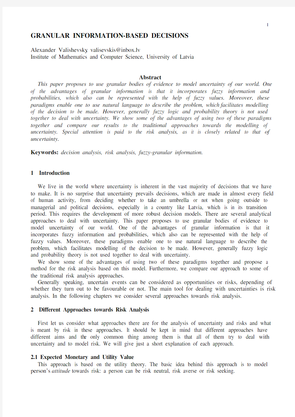
Several examples of utility function are presented in Figure 1. If the utility function is concave, which means that the increase in the utility decreases for bigger amount of money, the person is risk averse. If the utility function i s convex, the person is risk seeking, as the derivative of the utility function monotonically increases, thus higher monetary values result in higher acceleration of the utility value growth. If the utility function is linear, it means that monetary values are transformed into the utilities according to a linear function, thus the person is risk neutral and he can use the EMV to make his decisions.
Wealth
Figure 1. Different types of utility function
In this approach risk premium is used for the assessment of r isk. Technically speaking, risk premium is the difference between EMV and certainty equivalent, where certainty equivalent is amount of money equivalent to an uncertain situation. In other words, it is the price we would like to sell some lottery for. For example, if we are ready to sell for $50 a lottery where we have equal chances of winning $100 and loosing $25, then $50 is our certainty equivalent. Thus, the risk premium is amount of money we are ready to pay to avoid risk.
This approach is very subjective and its idea is to model person’s attitude towards risk. The assessment of risk based on risk premium is subjective as well.
One of the disadvantages of this method is that the assessment of the utility function takes pretty much time interviewing the expert. Further information on the utility theory you can find in [1].
2.2 Standard Deviation
Somewhat different approach towards the risk is exposed in [2]. This book considers risk of a portfolio. According to the idea exposed in this book, if you consider risk that is related to your portfolio, you should be concerned about the features of the probability distributions of the portfolio parameters (for example, share prices in the future). One of the features that you should be concerned with is dispersion, as it shows to what extent values of a parameter can vary.
If you try to model uncertain events using normal distribution, you should consider the standard deviation as the measure of the risk in your portfolio. Several issues and concerns are pointed out in [2]. For example, deviation does not "contain" only bad cases, e.g. when a share price goes down, but also cases when a share price increases and therefore the overall portfolio value increases.
Some of the disadvantages are evident: we have to model probability distribution for each share. Moreover, the real probability distribution is usually fitted to some theoretical model, which decreases the accuracy.
In this approach evaluation of the probabilistic parameters is used for risk assessment, not the investor’s subjective approach towards risk. However, assessment of probabilistic parameters (e.g. probability distributions) can be subjective, especially if there is not much historic data available.You can refer to [2] for further information on this approach towards risk analysis.
2.3 Entropy – Uncertainty about the Event
In this paper we consider an innovative approach towards risk assessment. In this approach we try to relate risk to the entropy.
Usually risk is related to the uncertainty of the future events. In other words, risk is related to the lack of knowledge about the future events. So it would be natural to define the risk as the amount of the lacking information. Thus, in this approach we adapt the idea that the risk reflects how much we do not know about the future.
Entropy is the basic notion in the information theory field. Informally we can define entropy as the measure of the uncertainty of some system that at a given moment can be in one of the states, where set of all the possible states is defined and the probability that system is in some state is known.
We can define entropy formally as follows. Let us assume that there are n different states that a system can be in:
s 1, s 2, … , s n .
With formula (1) we will denote that the probability that system is in state s i is p i .
P(S ~ s i ) = p i , i = 1 .. n
(1)If values of all p i in (1) are known, then system entropy can be calculated according to (2).
∑=?=n i i i p p H 1log .
(2)
For further information on entropy and information theory you can refer to a book on probability theory.
In the following chapters we consider the idea behind fuzzy and granular information and we show how the entropy can be calculated when values of the probabilities are interval valued.3 Fuzzy Information
In this section we will consider the idea behind fuzzy information. We will give just the basic details, but you are encouraged to refer to [4, 6] for further information on fuzzy sets and fuzzy logic.
The basic idea behind fuzzy logic is that in the real world one can rarely obtain numerically precise measurements, as measurement devices have only a limited precision and humans perceive and process information, which is fuzzy rather than precise numerically. For example, we usually say "there are a lot more small cars than big cars at a parking place" or "it is likely that it will rain today", but we rarely give a precise probability value, which denotes our confidence level that it will really rain.
Thus, we can use fuzzy values and quantifiers such as "big", "small", "old", "not very young", "most", "likely" etc. to describe perceptions of the events and processes in the real world. It is obvious that fuzzy values are more suitable in description of the real world, than the "common"
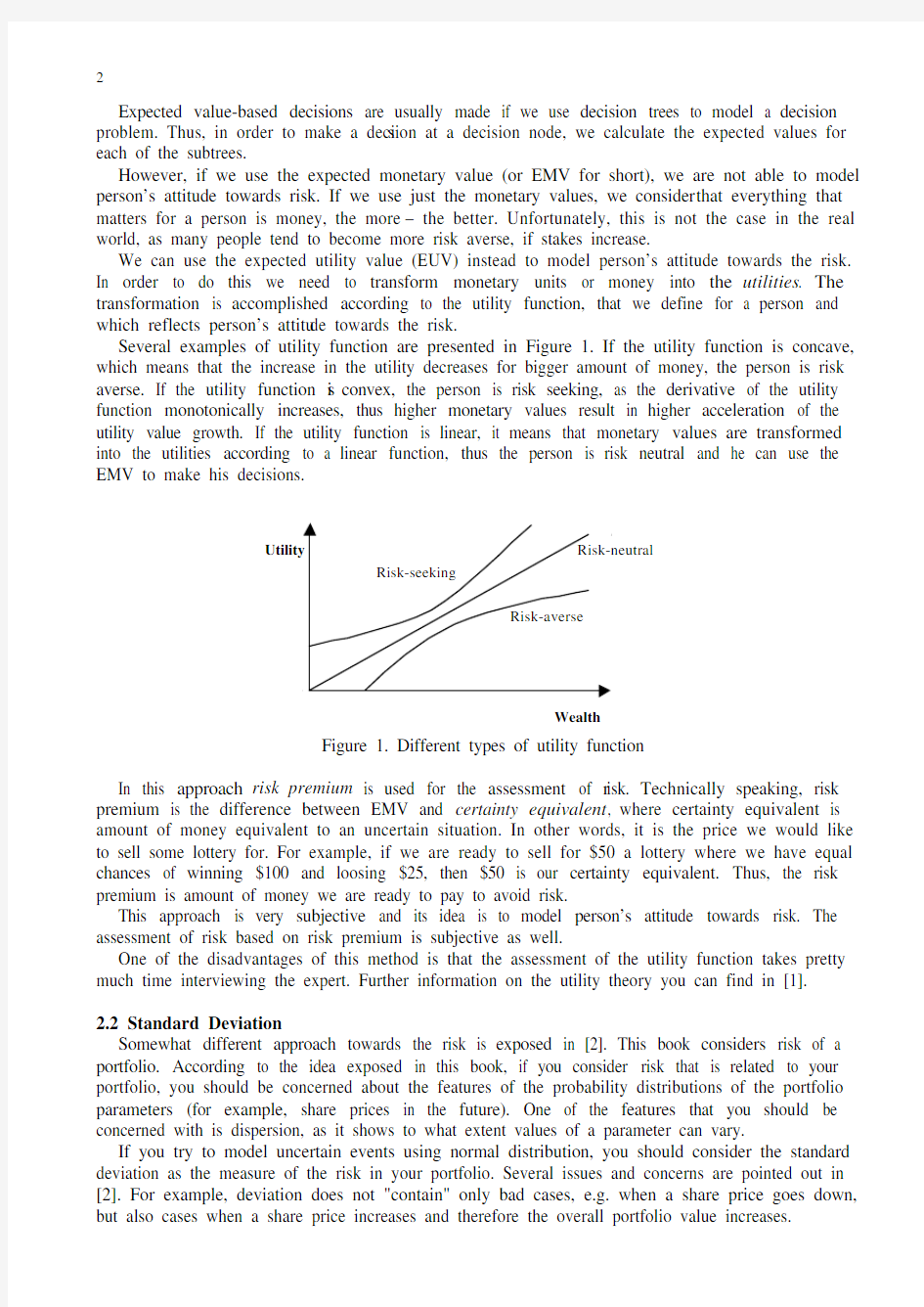
numbers or the crisp values. However, we need a lot more computational power if we are using fuzzy values. Each fuzzy value is given by a fuzzy subset represented with a membership function, which shows to what extent an element belongs to this set 1. For example, consider mem bership function of the fuzzy value "big" shown in Figure 2.
Figure 2. Fuzzy value "big"
As you can see in Figure 2, all values starting from 30 are "full" members of the fuzzy subset "big", but membership of values from 15 to 30 gradually increases from 0 to 1 (i.e. from non -membership to being full members).
Fuzzy logic is the basic component of the "soft computing" paradigm. In contrast to "hard" computing, we can use soft computing to do calculations when the data available is incomplete or imprecise, as well as if we do not need high degree of precision in our calculations, e.g. if they imply high costs of computing and/or modelling.
3.1 Fuzzy Granular Information
The idea of information granularity and its application in the context of fuzzy logic is presented in [5]. The idea of information granularity is very close to that of fuzzy information. Information is granular in the sense that, (a) the perceived information is fuzzy and, (b) the perceived information is granular with a granule being a bunch of values drawn together by similarity or indistinguishability.
In this paper conditioned π-granules are considered which are characterised by propositions of the following form:
i i i G Y u X g is then If ==?,
where G i is a fuzzy subset of V which is dependent on u i . Evidence E can be regarded as a collection of these granules:
E = {g 1, …, g N }.
Variable X assumes its value with a specified probability. Thus, evidence is probability distribution X P of conditional π-granules. Moreover, each granule can be regarded as conditional possibility ()i u X Y G i =Π=|. Hence, evidence can be regarded as conditional possibility distribution
()X Y |Π. Thus, evidence can be considered as the following construction:
()},{|X Y X P E Π=.
Given a collection of bodies of evidence },...,{1K E E E =, one would like to ask some questions
about the information contained in these evidences. The main question is: "what is the probability of (Y is Q )?", where Q is a fuzzy subset of V . The probability of such an event is an interval value in 1 Note, that in the crisp set theory, values of a membership function are either 1 or 0, i.e. an element either belongs to a
set or does not belong. In fuzzy set theory an element can belong to a set with a certain degree.
which the expected possibility )(E Q Π is regarded as the upper boundary, and the expected certainty )(EC Q is regarded as the lower boundary of the probability sought. In [5] the following formulae are proposed:
()
j i j i ij H G Q p Q ∩∩=Π∑sup )(E ,,
)(E 1)(EC Q Q ′Π?=,
where Q' is a complement of set Q . These formulae are for a special case in which there are two evidences in the system but it would not present any difficulty to induce a more general form of the formula.
In paper [3] you can find description of an adaptive network, which can be used to calculate the upper and the lower bound of the probability.
4 Uncertainty and Granular Information -Based Risk Assessment
As we have learnt from previous chapters, granular information can be represented with the help of conditional granules of the "IF…THEN…" form. In order to adapt this methodology to risk assessment, we can describe our problem domain with the help of such granules putting in the consequence ("THEN") part evaluation of some criterion, which is important for us and which is in direct or indirect relation to the risk inherent in our problem domain.
For example, if we are considering a project of constructing a power plant, we ought to consider to what extent it will influence the environment and the locality. Thus, we can describe our problem with a set of bodies of evidence made up of the following granules.
Evidence I, for the description of the distance to the closest inhabited area:
IF (plant is pretty close to inhabited area) with probability p 1,1 THEN influence is medium IF (plant is close to inhabited area) with probability p 1,2 THEN influence is moderately high IF (plant is very close to inhabited area) with probability p 1,3 THEN influence is high
Evidence II, for the description of the forecasted air pollution:
IF (air pollution is medium) with probability p 2,1 THEN influence is moderately high
IF (air pollution is not high) with probability p 2,2 THEN influence is low
Evidence III, for the description of the forecasted water pollution:
IF (water pollution is very low) with probability p 3,1 THEN influence is low
IF (water pollution is low) with probability p 3,2 THEN influence is medium
IF (water pollution is medium) with probability p 3,3 THEN influence is high
We can continue describing factors that can influence the evaluation of the chosen criterion and, as can be seen, we can incorporate our confiden ce in the values of these factors. Moreover, we can construct other sets of bodies of evidence, which describe evaluation of other criteria.
After we define bodies of evidence, we can calculate the probability that influence on the environment will be high or medium. Obtained probability will have an interval value [p min , p max ],which defines the lower and the upper bound of the probability.
We can calculate what are the probabilities that the criterion takes different values, e.g. "high", "low" etc. Moreover, we can consider different criteria.
In the following chapter we discuss how we can assess the uncertainty related to the probabilities obtained and how it can be related to risk.
4.1 Entropy and Interval Valued Probabilities
Let us consider how the en tropy can be calculated if we are dealing with the interval valued probability values. Obviously, the entropy itself will be interval valued.
In this section we induce a generalised definition of entropy, suitable for interval valued probabilities. As before, we assume that system can be in n states, but the probability that system is in i -th state is interval and is equal to [p i min , p i max ]. In case when probabilities are single valued rather than interval valued, it is required that probabilities sum to 1, i.e.
1=∑i i p
.(3)
If probabilities are interval valued, then this constraint can be rewritten as (4):
∑∑≤≤i i i i p p
max min 1.(4)
It is easy to show that (3) is a special case for (4), when p i min = p i max for each i . Moreover, if we define p i avg as p i avg = (p i min + p i max )/2, it can be shown that:
max min max min log log :i i i i i i p p p p p p i avg avg ?>??
We can find entropy for a system corresponding to the lower probability bounds p i min as follows:
∑=?=n
i avg i i p p H 1min min log ,and for the upper bounds p i max as follows:
∑=?=n
i avg
i i p p H 1max max log ,From (5) it follows that H max < H min . Moreover, as was mentioned above, entropy for a system with interval valued probability is interval valued as well and is equal to (6).
H = [H max , H min ].(6)
The obtained definition of interval valued is a generalisation of the "traditional" entropy of a system with single valued probabilities. However, it is not formal, as it was not shown that the basic properties of entropy are true also for interval valued entropy. However, from the definition of entropy by intuition it follows that such property as additivity holds for entropy defined according to (6). Thus, we can sum entropy values obtained for systems corresponding to different criteria. Lower and upper bounds of two system s should be summed separately to obtain the corresponding bounds of the summed entropy.
4.2 Incorporating Entropy and Risk Assessments
In the previous sections we described how we could use natural language to describe problem domain. After we construct f uzzy bodies of evidence, we can use them to calculate probability that criteria will take different values. Entropy values for systems corresponding to different criteria should be calculated separately and then summed according to the additive property of entropy. Obtained entropy is interval valued and we can use it to measure uncertainty of our problem domain and of evaluations of the criteria chosen.
One of the ways to do it is to find difference between the lower and the upper bounds of the entropy. The higher the difference, the higher the uncertainty and, thus, the risk.
5 Relation to Other Approaches
In the beginning of the paper we mentioned two other approaches towards risk analysis, viz., risk premiums in utility theory and standard deviations in portfolio risk evaluations.
As was mentioned before, risk premiums correspond to the price that a person is ready to pay to avoid the risk and are very subjective. In its turn, standard deviations are based on the probabilistic assessments of shares in a portfolio.
One of the disadvantages of both methods is that they require extensive subjective evaluations or probabilistic modelling, which take quite a lot of time. In the approach proposed in this paper, problem domain is being described with the help of natural language and the results obtained are being combined with the help of entropy.
Thus, this approach can be related to the utility theory approach, as all the evaluations are subjective and it can be related to the dispersion approach as well, as the risk assessment is based on the evaluation of uncertainty.
6 Conclusion
This paper shows how fuzzy granular information can be used in order to measure risk and uncertainty. The uncertainty assessment is based on the generalised definition of entropy. Moreover, we compare the approach described with other approaches, which are common in risk analysis.
One of the advantages of the approach proposed in this paper is that one can use natural language to describe problem domain, upon which the uncertainty is assessed. This is due to fuzzy logic upon which the approach is based, which enables one to use fuzzy rather than crisp values.
The approach towards risk analysis described in this paper can be used as a ready-to-use tool or it can be modified and extended in numerous ways, starting from the generalised definition of entropy to the assessment of uncertainty and the way the risk and uncertainty evaluations are incorporated.
Fusion of entropy and risk analysis is quite an innovative approach, and it is a subject of our current and most definitely future research.
Acknowledgement
I would like to thank Professor Arkady Borisov from Riga Technical University for the fruitful discussions on risk analysis that we had.
References
1.Clemen R.T. Making Hard Decisions, Duxbury Press, 1996.
2.Sharpe W.F., Alexander G.J. Investments, Fifth edition, Prentice Hall Int., 1995.
3. A. Valishevsky, A. Borisov, ANGIE: Adaptive Network for Granular Information and
Evidence Processing, Fifth International Conference on Applicati on of Fuzzy Systems and Soft Computing ICAFS-2002, Milan, Italy, September 2002, pp. 166-173.
4.Zadeh L.A. Fuzzy Sets and Systems. Proceedings of Symposium on System Theory,
Polytechnic Institute of Brooklyn, 1965, pp. 29-37.
5.Zadeh L.A. Fuzzy Sets and Information Granularity, Advances in Fuzzy Set Theory and
Applications, Editors: Gupta M.M., Ragade R.K et al., North-Holland Publishing Company, 1979, pp. 3-18.
6.Zadeh L.A. Fuzzy Logic, Computer Magazine, No.4, (1988), pp. 83-93.