Fast Traf?c Sign Detection and Recognition Under Changing Lighting
Conditions
Miguel′Angel Garc′?a-Garrido,Miguel′Angel Sotelo and Ernesto Mart′?n-Gorostiza
Abstract—In this work a system for traf?c-sign detection and classi?cation is shown.It is intended for both prohibition and obligation circular signs and for advertising triangular ones. The system is divided into three stages:?rst,detection,using the Hough transform from the information of the edges of the image;second,classi?cation,using a neural network,and third,tracking,making use of a Kalman?lter,which provides the system with memory.Some results are presented,obtained by real images recorded by only one camera placed on board a conventional vehicle,in sunny days,and also cloudy,rainy ones or at night,in order to show the reliability and robustness of the system.The average processing time is30ms per frame, what makes the system a good approach to work in real time conditions.
I.INTRODUCTION
The traf?c-signs detection and recognition systems have experimented an increasing interest in the last times,due to the importance of safety for drivers,occupants and pedes-trians.The detection systems constitute an aid to the driver, providing information to him about the signs appearing on the road.For instance,in case the maximum speed limit is overcome,an acoustic signal advising the driver could be activated.Speed-limit signals are the most important in this work as overcoming speed limits is one of the main causes of traf?c accidents,so,the?rst signs to be searched by our system are this kind of signs.Driving-aid is not the only use of these systems,traf?c-signs detection and recognition is also used for inventory,as shown in the AUTOCAT project [3].In this way,localization and classi?cation of traf?c signs is automated,also improving road maintenance.There are a lot of works about these topics but they seldom present results under adverse weather conditions,or at night.In this work,the results of a traf?c-signs detection and classi?cation system are shown,used for both circular and triangular signs, able to work in real time and showing ef?cient performance under adverse lighting conditions.
II.STATE OF THE ART
Three stages can be mainly distinguished in traf?c-signs recognition systems,as Gravila notes[17].These stages are detection,classi?cation and temporal integration or tracking. The analysis will be mainly focussed on detection,as it is the most delicate stage.
The authors are with the Department of Electronics,Escuela Polit′e cnica Superior.University of Alcal′a.Alcal′a de Henares,Madrid,Spain.Contact Author E-mail:garrido@depeca.uah.es A.Detection step
There are two forms of making the detection stage,not incompatible though;segmentation,using colour-information or analysis of the edges,obtained from grey-scale images. The former has two possible lines too,either working with the RGB colour space[9],[13],[16],[32]or working with those colour spaces that are less immune to lighting changes.In outdoor detection,lighting conditions cannot be controlled and so the RGB colour-space is highly dependant on the light.For this reason in all works,in which this space is used,relations between colour-components are used, what,to some extent,reduces this light-dependence.In this sense[20]makes a colour segmentation using a look-up table,generated off-line by a training process making use of a polynomial classi?er,so that pixels are labelled as ”red”,”blue”,”yellow”and”uncoloured”.Finally a colour-connected-components algorithm is applied(CCC),creating a database containing information as the perimeter,surface, colour,etc.of the region of interest,although not working in real time and neither providing results working with poor visibility or at night.In the latter type of works the HSI or HSL colour-space is used in order to reduce more the dependency on light[3],[11],[14],[18],[28].However,the captured image is not completely invariant against changes in the chromaticity of the received light.The hue component changes with shades,climatologic conditions and the traf?c sign age as explained by[31].Some works improving the colour segmentation have been carried out.For example[28] makes a detection based on a robust colour segmentation, followed by a hybrid parallel decision graph to evaluate the segmented regions of relevant colours.
Among the works in which edge-analysis starts from the grey-scale image,there may be highlighted[5],[8],[6],[17], [25],[27]although the detection algorithms are different. Gavrila[17]uses a template-based correlation method to identify potential traf?c signs in images;this involves the so-called distance transforms[7]starting form an edge-image,a matching with the template of those signs searched is carried out.These templates are organized hierarchically in order to reduce the number of operations,but however,this method has a high computational cost for a real-time system.Another work to be explained a bit more deeply is the one developed by[5],related to our work,because a variation of the Hough-transform is used[19].The method used by Barnes is based on[24],a fast method to detect points of interest using a system with radial symmetry.It uses the information of the magnitude and phase of the gradient of a grey-scale edge-
Proceedings of the IEEE ITSC 2006
2006 IEEE Intelligent Transportation Systems Conference
Toronto, Canada, September 17-20, 2006
TA6.3
image for different radii.Doing so,the method is able to detect only circular signs,more speci?cally,it is tested with 40and60-speed signs in real time performance.In order to detect triangular,square and octagonal signs Loy has used a similar technique in[25]increasing the computational cost so it cannot work in real time.In none of both works the system is tested in the rain or at night.
Comparing the methods based on colour segmentation with the ones based on shape-analysis it can be concluded that colour provides a faster focussing on the seeking-areas, but in practice precision is lower,due to the fact,for example, that blue and red colour spaces might overlap in those signs with white predominance,as in the end of speed limit ones, and there may arise problems in segmentation.Besides,as it has been already said,the measurement of the colour values can change considerably with lighting conditions.Moreover, region-growth methods that do not have information about the model tend to produce undesired problems of loss of colour information.In conclusion,those methods based on shape analysis are more robust against changes in lighting conditions.
B.Classi?cation step
The following stage is the classi?cation one;the resultant image from the?rst stage is analysed in this one by a classi?er that determines whether the previously detected candidate regions are actual traf?c signs or not.This is a much less critical step than detection,that is why in most of the works similar recognition methods are used.Neural networks,in their different topologies,are the most common tools employed.A map of the Kohonen is used in[26], while a cellular neural network is used in[1]able to classify triangular and circular traf?c signs,but the most commonly used topology is the backpropagation neural network used in [2],[13],[22],the input to the neural network is a normalized image containing the regions of interest previously detected, for example in[2]the image is18x18pixel-size,?fteen neurons in the hidden layer and three output neurons,so it can only distinguish between speed-limit,no-speed-limit sign and no-sign.Finally,another topology,widely used,is the radial-base neural network(RBF),used in[17],[23]and, as in the previous cases,a normalized image of the possible traf?c signs is used.Although neural networks constitute the main tool used in the classi?cation stage,it is not the only possibility,another huge group of works make use of template-matching techniques[27],[5],[29],make a normalized cross-correlation between the templates stored in data-base and the possible traf?c signs.For instance,Barnes applies the cross-correlation over a5x5window between the sign templates and the candidate signs.The classi?cation is applied only to two different speed-limit signs and only with three different radii for the search.
C.Temporal integration step
The last stage is the time-integration one,it enhances the reliability of the previous ones as it consists in providing the system with memory so that it takes into account not only
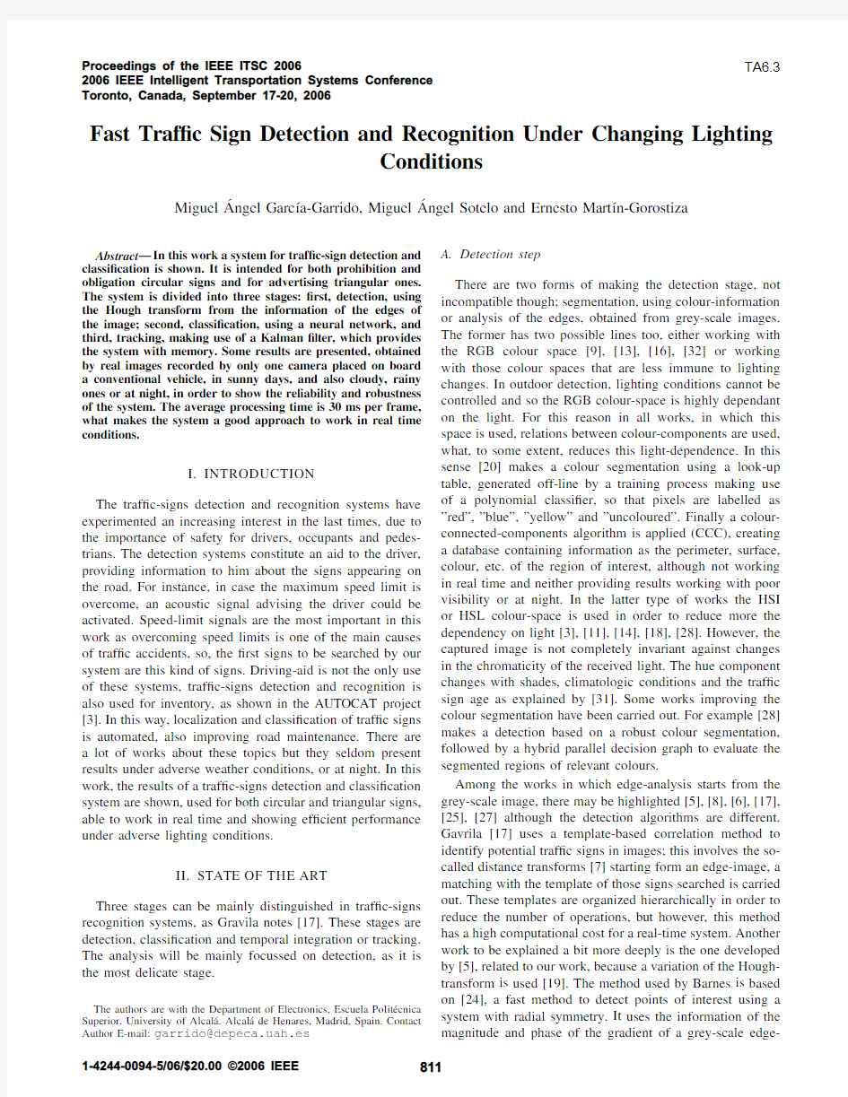
a Fig.1.Some images captured at night,in the rain and in a sunny day,with their corresponding histograms,in which threshold levels used to obtain the contour-image are shown.Contours meeting the restrictions are highlighted; Hough transform will be applied to them.
unique punctual instant for detection,but a whole sequence of images instead.To do so,the system must include the possibility of tracking.Not all the works in this area include this feature,but those in which this approach is implemented reach better results.Among the latter,[3],[17],[27],may be highlighted.All of them make use of an extended Kalman ?lter[21],and use the3D-position of the centre of the traf?c sign as the state-vector.
III.DETECTION
In this stage an analysis of the shapes obtained from an edge-image is carried out.In order to detect circular signs Hough transform for circumferences is used,while for triangular-signs detection the Hough transform for straight lines is used.The method works at day and night without the need of changing the algorithm,what is used thanks to the use of dynamic threshold-levels which change their values depending on the histogram distribution of the captured frame every time.
A.Contours Information
The algorithm used for edge detection is Canny method [10].This method preserves contours,what is very important for detecting traf?c signs using shape information because they are usually closed contours.The Canny operator uses the so-called”hysteresis”thresholding.With the aim of making the detection more reliable,we have chosen to adapt,the two canny-thresholds in a dynamic way,depending on the histogram-distribution of the image,so,the histogram has been divided into eight regions and a pair of threshold levels has been assigned to each one of the regions.In this way,the threshold levels assigned to the region with a wider value-distribution will be used,as it can be seen in?gure1.With this approach,it is possible to use the same algorithm either under good visibility conditions,in the day,or under less favourable conditions,at night,or in the rain.
The Hough transform could eventually reach a high computational cost if all the contours in the image were analyzed.However,all those contours that do not meet some requirements supposed to be typical of traf?c signs can be removed form the image.
The contours obtained applying Canny method are co-di?ed using the”chain code”[15].By making use of this codi?cation the area and the perimeter are obtained,and it can also be determined whether a contour is closed or not. The contours are accepted if they are closed contours,or
almost closed contours.They must also ful?l a certain aspect-
ratio constraint,showing similar width and height.Circular
traf?c signs,including stop one,as well as triangular ones,
meet these restrictions with high probability,as can be seen
in?gure1.Hough transform is only applied to accepted
contours after?ltered with the aforementioned restrictions,
so that the computational time is reduced.
B.Hough Transform
The classical Hough algorithm can be easily extended to
?nd any curves in an image that can be expressed analytically
in the form f(x,p)=0[4].Here,x is a point in the domain
of the image and p is a parameter vector.
Hough transform for straight lines is applied in order to
detect triangular signs.A straight line in the xy-plane with a
distance to the originρand the angle of the normal line to
this straight line passing through the origin,with the abscissa
axisθcan be expressed as(1).
x·cos(θ)+y·sin(θ)=ρ(1) Where the parameter space,p=(ρ,θ),must be quantized.
If the origin of the co-ordinate system is placed in the centre
of the image,the largest possible distance between a point
in the image and the origin is R.Hence,in order to generate
any straight line of an image,ρmay be varied between?R
and+R,andθmay be varied between0andπradians.
The parameter-space is quanti?ed and expressed in a2D
accumulation matrix A with dimensions m x n,where m is
the number of values assigned toρand n is the number
of values assigned toθ.For straight lines detection all the
elements of A are initially set to zero.So,an element
A rt(ρr,θt)is incremented by1for every feature point (x i,y i)in the image-domain,contained in the straight line with parameters(ρ,θ)as expressed in(2),and as shown
in?gure2,where a precision margin is introduced to
compensate for quantization error when digitizing the image
[30].
|x i·cos(θt)+y i·sin(θt)?ρr|< (2) The aim is detecting three straight lines intersecting each other,forming a60degrees-angle.It must be observed that, as long as the number of straight lines intersecting each other might be very large if the Hough transform was applied to the whole image,more than the actual triangles existing in the image would be https://www.doczj.com/doc/9d5042665.html,ing Hough transform neither the beginning nor the end of a straight line is known.In order
ρ
R
-R
(ρrθt)
0π
θt
r
Fig.2.Hough transform for straight lines.
Fig.3.Straight lines detected using Hough transform,applied to the whole image(left)applied to each contour,one by one(right).
to overcome this handicap in this work the strategy is to apply the Hough transform to every contour,one after the other.In this way,only those triangles existing actually in the image are detected,as shown in?gure3,reducing the computational time too.
A similar strategy is followed for circular sign detection. Hough transform for circumferences is applied to detect circular signs and the stop sign too.Although the stop sign is octagonal,the difference between octagonal and circular signs is very slight,and the former ones are also accepted.A circumference in the xy-plane with center(χ,ψ)and radius ρcan be expressed as(3).
(x?χ)2+(y?ψ)2?ρ2=0(3) Where the parameter space,p=(χ,ψ,ρ),must be quantized.The accumulator matrix A is the representation of the quantized parameter space.For circumference detection the accumulator A will be a three-dimensional matrix with all elements initially set to0.The element A rst(χr,ψs,ρt) is incremented by1for every feature point(x i,y i)in the image-domain,contained in the circumference with centre (χr,ψs)and radiusρt as expressed in(4),and as shown in ?gure4where a precision margin for the radius is intro-duced to compensate for quantization error when digitizing the image[30].
|(χr?x i)2+(ψs?y i)2?ρ2t|< (4) For circular-objects detection the same criteria are follo-wed as in the case of straight lines.Hough transform is applied contour by contour,so that those contours corres-ponding to other shapes but not signs do not affect the detection of the latter ones,so,feasibility is increased too and computing time is reduced considerably,as with the classic Hough transform all the pixels are analyzed as possible centres and the threshold must be?xed.This implies that
Fig.4.Hough transform for circumferences.
more circumferences than the real existing ones are detected. In order to avoid detecting inexistent circumferences the analysis of every contour is performed and the Hough trans-form is applied only to the points belonging to the contour under study.Hence,the information of a contour obtained already in a previous stage is used and the centre of the circumference is searched in the environment of the centroid of the corresponding contour.In this way the number of iterations is considerably lowered without loss of reliability. On the other hand,a thresholding can be done,adapted to every contour;if the contour has a large amount of points its threshold is higher than if there are less points in it.With this,seeking circumferences only with certain radius,as it happens in[5]is avoided.All these considerations make detection time to be very short,making the system able to work at a processing-speed between5and50frames per second,depending on the number of contours detected.
IV.CLASSIFICATION
Making use of the information obtained in the detection stage,where it is known if the possible signs are circular or triangular ones,two different neural networks have been implemented for recognition.One of them identi?es whether it is a triangular sign or not,and its type,and the other one recognizes the circular signs,including the stop-one.Both of the neural networks are backpropagation neural networks, where the input to it is a32x32pixel-size normalized image of the candidate sign.Every type of sign,wanted to be detected,has a normal distribution probability-density function,centred in a neuron and with a deviationσ=1. To identify a sign,a correlation between the values of the output-layer neurons and the normal distribution is carried out,and depending on which neuron the maximum is reached at,and if it overcomes a certain threshold,it will be classi?ed as a sign,or else as no-sign.Besides,the value of the correlation indicates the probability that the detected sign is a correct sign.The steps
are shown in the block-diagram in?gure5.
It must be noted that the networks have been trained to recognize the speed-limit and end-of-speed-limit,stop, forbidden-overtaking and end-of-forbidden-overtaking signs for circular ones,while for triangular signs,the give way sign,and dangerous-curves advertisement are considered. Real time tests have been carried out working with a data-
Fig.5.Block diagram of the classi?cation stage.
base,from which the system is able to distinguish among more than a thousand signs,reaching a99%classi?cation-rate.
V.TEMPORAL INTEGRATION
Once the sign has been detected and classi?ed it is necessary to track it,so that the system is provided with memory and it is not necessary to do the classi?cation with all the frames,and once the candidate is classi?ed the type of sign would be shown if the recognition was positive,or else it would be labelled as no-sign in case the recognition was negative,in order to reduce the seeking time in next frames.To perform the tracking a Kalman?lter has been implemented,this?lter makes an estimation of the evolution of the system and compares it with the actual output;in this way its estimation is improved as it keeps on executing, making the algorithm to be recursive.Tracking is performed with circular and triangular signs,and in both cases the state-vector is(5).
x(x k,y k,r k)T(5) Where the components(x k,y k)of the state-vector are, for circular signs,the centre of the detected circumference, and for triangular ones the centre of the circumscribed circumference,while the component r k is the radius of these circumferences.An example of an application of Kalman ?lter is shown in?gure6,where it can be seen how a tracking of a sign under different lighting conditions is done.
VI.RESULTS AND CONCLUSIONS
A real time-algorithm for traf?c signs detection and re-cognition has been shown.The algorithm is able to detect any kind of signs but the informative ones,using a similar technique for all of them,Hough transform,making the algorithm very robust and reliable.The system works with one only camera mounted on the windscreen of the car, as shown in?gure7.Several tests have been conducted, placing the camera in different positions on the windscreen, and it has been concluded that the placement of the camera is not decisive,but orientation is,thus affecting the quality of detection.The best arrangement is to place the camera pointing towards the same direction and sense of the car so that signs are seen orthogonally to the egomotion direction
Fig.6.Traf?c sign tracking under different lighting conditions using the Kalman ?lter.From left to right and up to down:end of forbidden overtaking at night.Same signal with rain drops on the car windscreen.Left bend warning sign and speed limit sign in a cloudy day.Give-way sign in a sunny
day.
Fig.7.One camera mounted on the windscreen of the car.
and thus suffering the least possible distortion.Should a circular sign be captured non-orthogonally by the camera,it would be seen as an ellipse in the image and would not be so neatly detected.However,Hough transform can be extended to ellipses,but it would be necessary to add two new parameters in the parameter-space with respect to the transform for circumference used in this work.This technique has been tested in fact,and it was noticed that the average processing time was 2seconds,so the system could not operate in real time.It is important to realize that detecting circumferences but not ellipses is in fact a simpli?cation of the method,but it does not imply a poorer performance at all.On the contrary,an elliptical shape in the image captured,if it happened to correspond to a sign,would be placed with high probability in another road with other direction,for instance in a crossroads.So,only those signs detected as circular are placed in our road in the egomotion direction.
The system has been empirically tested under different lighting conditions,in sunny or cloudy days,in the rain and at night,as it can be seen in the sequence of images in ?gure 8.An important aspect to be highlighted is that either the detec-tion algorithms,or the classi?cation and tracking ones are the same in every case because they are adaptive.Adaptation is achieved mainly due to two factors,?rst the use of adaptive thresholds applied to canny algorithm to obtain contours,that change their values depending on the histogram function at any time,and second,the application of Hough transform
TABLE I
R ESULTS OF TEST MADE .
traf?c sign amount detecting recognition speed limit 43597.2%98.5%warning
312
94.3%
97.2%
depending on the information received form every candidate contour.Tracking,using the Kalman ?lter improves clearly the computational time and also provides the system with memory what makes possible classifying a sign only once.On the other hand,recognition stage,solved by using a neural network,is eventually less critical than detection one;speed limit and warning traf?c sings have been chosen in order to test the system,although it can be extended to the rest of traf?c sings.The results of this test are shown in table I.As future work,it would be of high interest to integrate this system with a positioning one as the GPS,in order to be used for inventory and sign maintenance.It would also help distinguishing whether the detected sign is aimed to the driver carrying the system.
A CKNOWLEDGEMENTS
This work has been supported by grants DPI2002-04064-C05-04and DPI2005-07980-C03-02from the Spanish Mi-nistry of Education and Science and FOM2002-002from the Spanish Ministry of Public Works.
R EFERENCES
[1]G.Adorni,V .Dandrea,G.Destri and M.Mordoni,”Shape searching
in real world images:a CNN-based approach,”Fourth Workshop on Cellular Neural Networks and their Applications ,IEEE June (1996)[2]Y .Aoyagi,T.Asakura,”A study on traf?c sign recognition in
scene image using genetic algorithms and neural networks,”22nd International Conference on Industrial Electronics,Control,and Ins-trumentation ,IEEE August (1996)
[3]P.Arnoul,M.Viala,J.P.Guerin,M.Mergy,”Traf?c signs localisation
for highways inventory from a video camera on board a moving collection van,”Intelligent Vehicles Symposium ,Proceedings of the 1996IEEE,pp.141-146,Sept (1996)
[4] D.Ballard,”Generalizing the Hough transform to detect arbitrary
shapes,”Pattern Recognition ,vol.13,no.2,pp.111-122,(1981)[5]N.Barnes,A.Zelinsky,”Real-time radial symmetry for speed sign
detection,”Intelligent Vehicles Symposium ,IEEE,pp.566-571,June (2004)
[6] B.Besserer,S.Estable,B.Ulmer,D.Reichqardt,”Shape classi?cation
for traf?c sign recognition,”First International Workshop on Intelli-gent Autonomous Vehicles ,IFAC April (1993)
[7]G.Borgefors,”Distance Transformations in Digital Images,”Computer
Vision,Graphics and Image Processing ,pp.344-371(1986)
[8]U.Buker,B.Mertsching,”Parallel evaluation of hierarchical image
databases,”Journal of Parallel and Distributed Computing ,pp.141-152,(1995)
[9]S.Buluswar,B.Draper,”Color recognition in outdoor images,”Sixth
International Conference on Computer Vision ,IEEE January (1998)[10]J.Canny.”A Computional approach to Edge-Detection,”IEEE Tran-sactions on pattern Analysis and Machine Intelligence ,vol 8,pp.679-700,(1986)
[11] E.De Micheli,R.Prevete,G.Piccioli,M.Campani,”Color cues for
traf?c scene analysis,”Intelligent Vehicles ’95Symposium ,pp.466-471Sept (1995)
[12]R.Duda and P.Hart,”Use of the Hough transform to detect lines and
curves in pictures,”Communications of the ACM ,vol.15,no.1,pp.11-15,(1972)
Fig.8.Sequence of real road images under different weather and light conditions,where circular and triangular signs are detected.
[13] A.de la Escalera,L.Moreno,M.A.Salichs,J.Ma.Armingol,”Road
traf?c sign detection and classi?cation,”IEEE Transactions on Indus-trial Electronics,pp.848-859(1997)
[14] C.Y.Fang,C.S.Fuh,S.W.Chen,and P.S.Yen,”A road sign
recognition system based on dynamic visual model,”in Proc IEEE Conf.on Computer Vision and Pattern Recognition,vol.1,pp.750-755(2003)
[15]H.Freeman,”On the encoding of arbitrary geometric con?gurations,”
IRE Transactions on Electronic Computers,vol.10,(1961)
[16]M.A.Garc′?a,M.A.Sotelo,E.Mart′?n-Gorostiza,”Vision-based Traf?c
Sign Detection for Assisted Driving of Road Vehicles,”Informatics in Control,Automation and Robotics(ICINCO),vol2,pp.19-24, September(2004)
[17] D.M.Gavrila,”Traf?c Sign Recognition Revisited,”Proc.of the21st
DAGM Symposium fr Mustererkennung,pp.86-93,Springer Verlag, Bonn,Germany,(1999)
[18]T.Hibi,”Vision based extraction and recognition of road sign region
from natural colour image,by using HSL and coordinates transforma-tion,”29th International Symposium on Automotive Technology and Automation,Robotics,Motion and Machine Vision in the Automotive Industries,ISATA June(1996)
[19]P.Hough,”Method and means for recognizing complex patterns,”Dec.
181962.U.S.Patent3,069,654.(1962)
[20]R.Janssen,W.Ritter,F.Stein,S.Ott,”Hybrid approach for traf?c
sign recognition,”Intelligent Vehicles Symposium,IEEE July(1993) [21]R.E.Kalman,”A New Approach to Linear Filtering and Prediction
Problems,”Transaction of the ASME-Journal of Basic Engineering, pp.35-45March(1960)
[22] D.S.Kang,N.C.Griswold,N.Kehtarnavaz,”An invariant traf?c
sign recognition system based on sequential color processing and geometrical transformation,”Southwest Symposium on Image Analysis and Interpretation,IEEE April(1994)
[23]U.Kressel,F.Lindner,C.Whler,and A.Linz.”Hypothesis veri?cation
based on classi?cation at unequal error rates,”In Submitted to ICANN, (1999)
[24]G.Loy,A.Zelinsky,”Fast radial symmetry for detecting points of in-
terest,”Pattern Analysis and Machine Intelligence,IEEE Transactions on,V olume25,Issue8,pp.959-973,Aug.(2003)
[25]G.Loy,N.Barnes,”Fast shape-based road sign detection for a driver
assistance system,”Intelligent Robots and Systems,(IROS2004).
Proceedings.2004IEEE/RSJ International Conference on,V ol.1,pp.
70-75(2004)
[26]R.C.Luo,H.Potlapalli,D.Hislop,”Neural network based landmark
recognition for robot navigation”,International Conference on Indus-trial Electronics,Control,Instrumentation,and Automation,Power Electronics and Motion Control,IEEE November(1992)
[27]G.Piccioli,E.de Micheli,P.Parodia,M.Campani,”Robust method
for road sign detection and recognition,”Image and Vision Computing pp.209-223,(1996)
[28]L.Priese,https://www.doczj.com/doc/9d5042665.html,kmann,V.Rehrmann,”Ideogram identi?cation in a
real-time traf?c sign recognition system,”Intelligent Vehicles Sympo-sium,IEEE September(1995)
[29]P.Seitz,https://www.doczj.com/doc/9d5042665.html,ng,B.Gilliard,and J.C.Pandazis.”The robust
recognition of traf?c signs from a moving car,”In Proc.13th DAGM Symposium on pattern recognition,pp287-294,(1991)
[30]S.D.Shapiro,”Properties of transforms for the detection of curves in
noisy image,”Computer Graphics and Image Processing,vol.8,pp.
219-236,(1978)
[31]M.Thomson and S.Westland,”Colour-imager characterization by
parametric?tting of sensor responses,”Color Reserch and Application, col.26,no.6,pp442-449,Dec.(2001)
[32]M.M.Zadeh,T.Kasvand,C.Y.Suen,”Localization and recognition
of traf?c signs for automated vehicle control systems”,Intelligent Transportation Systems,SPIE(1998).
一、高速球综述 高速球是一种智能化摄像机前端,全名叫高速智能化球型摄像机,或者一体化高速球智能球,或者简称快球,简称高速球。高速球是监控系统最复杂和综合表现效果最好的摄像机前端,制造复杂、价格昂贵,能够适应高密度、最复杂的监控场合。 二、高速球的结构及原理 高速球是一种集成度相当高的产品,集成了云台系统、通讯系统、和摄像机系统,云台系统是指电机带动的旋转部分,通讯系统是指对电机的控制以及对图象和信号的处理部分,摄像机系统是指采用的一体机机心。而几大系统之间,起着横向的连接的是一块主控核心cpu和电源部分。电源部分通过与各大系统之间供电,很多地方是采用的二极管、三极管等微电流供电,而核心cpu是实现所有功能正常运行的基础。 高速球的原理实际上大致就是以上所说的,而具体来说,高速球采用“精密微分步进电机”实现高速球的快速、准确的定位、旋转。所有这一切都是通过cpu发给的指令来实现的。然后将摄像机的图象、摄像机的功能写进高速球的cpu,实现在控制云台的时候,将图象传输出来,并且能将摄像机的很多功能,例如白平衡、快门、光圈、变焦、对焦等功能同时实 现控制。 一般高速球都分为球心部分、外壳部分及配件部分。任何厂家的高速球,都有一个用机架把包一体机机心、控制解码主板和电机云台系统的统一起来的球心部分,然后球心部分跟外壳用螺丝或者别的方式连接起来,球心是核心部分,外壳一般有多种外观,比如派尔高外观、松下外观、和自己设计的外观。外壳一般都是采用铝合金,也有塑料的,铝合金的一般又分为铸造和冲压的两种外壳。铝合金的比塑料的好,冲压的比铸造的好。下外壳是透明罩部分,透明罩必须采用光学透明罩,才能保证通光率和图象无变形,同时还要考虑防老化、防破坏、防尘等问题。配件部分一般包括支架部分,加热器部分,扇热部分。支架包括壁装
压力单位及换算 注:毫米水柱是指4摄氏度状态的水柱高度,毫米汞柱是指0摄氏度状态的水柱高度。 1mmAg = 9.80665Pa = 0.0980665hPa 1atm = 760 mmHg = 1013hPa 1mmAg = 0.0735793mmHg 一、压力(pressure)为单位面积所承受的力 压力:绝对压力、表压力、大气压力。相互关系:绝对压力=表压力+大气压力 * 绝对压力(Absolute Pressure):当压力表示与完全真空的差。测量处的实际压力。 * 表压力(Gage Pressure):当表示其气体数值与该地域大气压力的差值。 * 大气压力:(Pressure Atmospheres)由大气重量所产生之压力,标准大气压力为29.92″
寸汞柱压力. 风压:包括全压(P.T)=静压(Ps)+动压(Pv)即速度压(V.P)。 Total Pressure=Static Pressure+Dynamic(Velocity)Pressure。 风机所产生之压力,均以水柱来测量,因风机使用之压力均很小;而水银之密度很大(1m mHg=13.6mmAq)使用水银柱(mmHg)来测量时,读数不太明显,故多采用水柱(mmAq 或mmH2O)来测量或计算。 如:采用水银柱表示时,760mm水银柱=760 mmHg 。 选用水柱表示时,100mm水柱=100 mmAq 。=(4″w g) Aq为拉丁文Aqua之简称。1mmAq之压力约=1kg/m2 。 1标准气压=1.0332kgf/cm2=10.34mAg=760mmHg=29.92inHg寸汞柱 (Kg为质量单位,Kgf为重量单位。) 二、压力常用单位(CNS 7778)(注2) 大气压Atm.(Pressure Atmospheres)=760mmHg 。 压力之表示,以大气压为准,高于此压力者为正压,低于此压力者为负压;速度压必为正压。 吋水银(汞)柱:(″Hg) 3.377=KPa 。 吋水柱:(″Wg or H2O) 0.249=KPa 。 呎水柱:(′Wg) 2.989=Kpa 公斤/平方公尺:kg/m2 ;kg/cm2 98=KPa (1mmAq=9.797Pa<9.8Pa=9.8Pa) 摩擦阻力 ″wg/100′ 8.2=Pa/m ″wg/100′ 98.1=Pa/m mAq 9.8=KPa ;mmAq 0.0098=KPa ;mmAq/m 9.8=Pa/m 重量:磅/平方英吋(lbs/in2或Psi 6.895KPa)。(1Kg=2.205lbs) 三、术语之意义(CNS 7778B4046)(注2) 1.全压…*送风机全压,是由于送风机所得之全压增加量,以送风机进口及出口之全压差表示 。 * 于导管内之任意断面处,气流均具有静压与速度压,二者之代数和称为全压。 2.静压…*送风机静压是指由送风机全压,减去送风机排出口动压而言。即全压减动压后之压力,称为静压。
摄像机录制方式详解 磁带类 VSH 格式:现在不用很少见的:(这种格式是JVC公司1976年推出的,我国家庭中使用的 像机绝大多数是这种格式。 S-VHS 格式:这是VHS格式的高带方式,亮度信号信噪比提高4dB 以上,使S-VHS 格式的图像清晰度达到水平400线,也能应用于广播业务领域。 Betamax 格式:这是索尼公司研制的,对抗VSH的。 VHS-C 格式:磁带盒几乎是VHS 型磁带盒大小的一半。8mm 型/Hi8 型等。 1.U型机:3/4英寸专业录像机(有高/低带)。磁鼓上装有两个相隔180度的(Y/C)视频录放磁头,每旋转一周两个磁头各记录一场信号,磁头鼓的旋转频率为25Hz。磁鼓直径比较大,记录速度较高视频磁迹较宽,相邻迹间有空白保护区。音频磁迹共有两条,控制磁迹为一条,记录控制脉冲(CTL)信号。 2.Betacam SP型录像机:使用1/2英寸金属磁带。它采用分量记录两对磁头同时而又独立地在磁带上分别记录亮度和色度信号。色度信号采用时间轴压缩(CTDM)技术,克服了清晰度降低,彩色失真,信杂比降低的缺点。 3.MⅡ格式分量录像机:了解资料不多。 4.DV 数码格式:DV(Digital Video Cassette)。DV 系统的亮度信号的取样频率高达13.5MHz,而色信号的取样频率也可达3.375MHz,清晰度理论上可达500线,视频信噪比可达54dB。在音响方面也很考究,有16比特/48千赫 44.1千赫 32千赫两声道及12比特/32千赫四声道几种规格。 5.DVCPRO 格式:DVCPRO是1996年松下公司在DV格式基础上推出的一种新的数字格式。它采用 4:1:1取样,5:1压缩,18微米的磁迹宽度。1998年又在 DVCPRO的基础上推出了DVCPRO50,它采用4:2:2取样,3.3:1压缩。1999年开始推出更高级的产品DVCPRO100,又称DVCPRO HD,向数字电视的更高水准--高清晰度电视领域发展。DVCPRO 家族可满足现场演播室以及更多广播级和专业级应用的需要。 6.Digital-S 格式:是日本JVC公司于1995年4月推出的一种新型的广播专业级数字分量录像机(也称D-9格式)。它是以S-VHS技术为基础开发的具有高效编码数字技术S格式的录像标准,它可以重放S-VHS的图像信号,录像带宽度为12.7毫米(1/2英寸),采用4:2:2取样,8BIT量化,采用帧内3.3:1压缩,视频数据率为50MBPS。可记录4路音频,每路48KHZ取样,16BIT量化。 7. DVCAM 格式:1996年推出了 DVCAM 格式的数字设备.采用5:1的压缩比,4:2:0 (PAL) 取样方式,8比特数字分量记录,保证了画面的高质量,并可兼容重放家用数字 DV 录像带,具有优越的性价比。 8.Betacam-SX 格式:它采用了MPEG-2 MP@ML 的扩展4:2:2P@ML 标准。在保证高图像质量的同时有较高的压缩比(10:1). 9.Digital-Betacam 格式:SONY公司于1993年推出 Betacam数字分量录像机。采用1/2英寸金属带。视频信号采用4:2:2取样,数字输入10BIT量化,模拟输入8BIT量化,帧内2:1数据压缩.
压力单位换算表
高度。 1mmAg = 9.80665Pa = 0.0980665hPa 1atm = 760 mmHg = 1013hPa 1mmAg = 0.0735793mmHg 一、压力(pressure)为单位面积所承受的力 压力:绝对压力、表压力、大气压力。相互关系:绝对压力=表压力+大气压力 * 绝对压力(Absolute Pressure):当压力表示与完全真空的差。测量处的实际压力。 * 表压力(Gage Pressure):当表示其气体数值与该地域大气压力的差值。 * 大气压力:(Pressure Atmospheres)由大气重量所产生之压力,标准大气压力为29.92″寸汞柱压力. 风压:包括全压(P.T)=静压(Ps)+动压(Pv)即速度压(V.P)。 Total Pressure=Static Pressure+Dynamic(Velocity)Pressure。 风机所产生之压力,均以水柱来测量,因风机使用之压力均很小;而水银之密度很大(1mmHg=13.6mmAq)使用水银柱(mmHg)来测量时,读数不太明显,故多采用水柱(mmAq或mmH2O)来测量或计算。 如:采用水银柱表示时,760mm水银柱=760 mmHg 。 选用水柱表示时,100mm水柱=100 mmAq 。=(4″wg) Aq为拉丁文Aqua之简称。1mmAq之压力约=1kg/m2 。 1标准气压=1.0332kgf/cm2=10.34mAg=760mmHg=29.92inHg寸汞柱 (Kg为质量单位,Kgf为重量单位。) 二、压力常用单位(CNS 7778)(注2)
《2D-3D 定位算法》笔记 中英对照: 世界坐标系或实体坐标系(3D):object coordinate system 。 摄像机坐标系(3D): camera coordinate system 。 图像坐标系(2D): image coordinate system ,在摄像机坐标系下取x 和y 坐标即为图像坐标系。 2D-3D 点对:2D-3D correspondences ,根据投影变换将3D 点投影为2D 点。 平移变换:translation projection 旋转变换:rotation projection 比例变换:scale projection 透视投影变换:perspective projection 正交投影变换:orthographic projection 2D-3D 定位算法:根据 已给出的若干对 3D 点p i (在世界坐标系或实体坐标系下)和 相对应的 2D 点p i '(在图像坐标系下或在摄像机坐标系下取x 和y 坐标),求出之间的投影变换矩阵(旋转变换和平移变换)。 文献1: 《A Comparison of 2D-3D Pose Estimation Methods 》 文献2: 《A Comparison of Iterative 2D-3D Pose Estimation Methods for Real-Time Applications 》 文献3: 《计算机视觉》-马颂德 一、CamPoseCalib(CPC) 1、基本思想:根据非线性最小二乘法,最小化重投影误差求出投影参数 ),,,,,(γβαθθθθθθθz y x =。 2、算法过程: (1)已给出若干点对)'~ ,(i i p p ,其中i p 是实体坐标系下的3D 点,' ~i p 我理解为事 先给出的图像坐标系下的2D 点,应该是给出的测量值 。 (2)将i p 先经过旋转变换 i z y x p R R R ???)()()(γβαθθθ 和平移变换 T z y x ),,(θθθ ,得 到 摄 像 机坐标系下的点 i z y x T z y x i p R R R p m ???+=)()()(),,(),(γβαθθθθθθθ 。 (3)再将像机坐标系下的点),(i p m θ进行透视投影变换得到图像坐标系下的2D 点:
常用压力压强单位换算表 为方便记忆,可以简化为如下规律: 1. 1atm=0.1MPa=100KPa=1公斤=1bar=10米水柱=14.5PSI 2. 1KPa=0.01公斤 =0.01bar=10mbar=7.5mmHg=0.3inHg=7.5torr=100mmH 2O=4inH 2 O 3. 1MPa=1N/mm2 常用压力压强单位换算(atm mmHg mH2O Pa bar)(2008-05-22 16:43:11) 标签: 1个标准大气压=76厘米水银柱高=1.01×10⁵帕=1010mbar=10.336米水柱高测定大气压的仪器:气压计(水银气压计、盒式气压计)。
大气压强随高度变化规律:海拔越高,气压越小,即随高度增加而减小,沸点也降低。 毫巴(mbar或mb) 概述 用单位面积上所受水银柱压力大小来表示气压高低的单位。物理学上,压强的单位是用“巴”表示的:每一平方厘米面积上受到一达因的力,称为一巴。在气象上,嫌这个单位太小,取1,000,000达因/平方厘米为1巴,以巴的千分之一作为气压的单位,称为1毫巴。一毫巴为一巴的千分之一,等于0.75毫米水银柱高的压力。现改称“百帕”。1毫巴等于100 帕(hPa)。 发明 毫巴的概念由Napier Shaw先生于1909年发明, 于1929年为国际所接受。Unicode符号为“mb”(㏔)。 分析 1毫巴表示在1平方厘米面积上受到1000达因的力。例如,气压为1000mb,表示当时大气柱在每平方厘米面积上的力有1,000,000达因。 达因是力的单位,在厘米-克-秒制中,它代表作用于一克质量的物体上,使物体以1cm/秒2的速度发生运动的力。达因是很小的一个力。夏天我们看到的蚂蚁叼着小小的草梗所付出的力,就有100达因。可见,一达因的力之小了。 毫米与毫巴可以相互换算。根据压强与水银柱高度的关系式:P(压强)=h(水银柱高度) ×d(水银在0℃时的密度) 气压为水银柱高度1毫米=0.1厘米×13.596克重/厘米3=1.3596克重/厘米2 在纬度45°的海平面上,1克重=980.6达因 故:1毫米=1.3596×980.6=1333.22达因/厘米2=1.33322毫巴=3/4毫巴 根据这个关系,气压为760毫米时相当于1013.25毫巴,这个气压值称为一个标准大气压。 平均海平面压力是1013.25 hPa (mbar)。这个值随着高度的上升而下降。 应用 毫巴是一个用于测量压力的物理单位。毫巴不是SI单位. SI单位为帕斯卡 (帕), 1mbar = 100 Pa = 1 hPa = 0.1 kPa. 虽然如此, 但毫巴在很多场合仍然是一个常用单位。
PTZ摄像机的技术优势和发展趋势 ——深圳市保千里电子有限公司安防渠道部总监吴雪芳传感器和计算机计算的发展影响了新型计算机网络和处理框架的发展。其中,中小型视频监控网络已经被广泛应用。 在现代监控系统中,多摄像机追踪问题中的一个主要挑战是如何在不同的FOV下保持目标标识的连续性。尽管静态摄像机网络可以为监控任务覆盖一个广阔的区域,但为了增加摄像机监控区域增加摄像机可视角度时,图片分辨率会因此降低;当不存在重叠的FOV时,信号处理必须仍然在单个数据源上执行。因此,PTZ摄像机的引入,为摄像机网络的发展带来了全新的应用优势。 球型摄像机(PTZ Dome)是一种一体化球型摄像机,具有运转速度快、光学变焦、定位精确、控制方式灵活等特点,随着整个监控行业数字化、网络化、高清化发展的进程,网络PTZ摄像机在产品的开发上也迈入了一个新的阶段,高清PTZ摄像机成为监控行业新的热点。其主要具有以下四大应用优势。 以太网供电 ALL IN ONE,即一个网线实现所有数据的传输,这是网络监控的一个重要优势。以太网供电IEEE 802.3af(在POE交换机端的电压是48V DC,最大功率15.4W),只适合给固定网络摄像机和固定半球摄像机进行供电。 High PoE ,802.3at在电压范围支持50-57V DC,标程为53VDC,最大功率支持30W,完全可给快球摄像机及其护罩供电。通过High PoE,网络快球不需要任何视频线、音频线、控制线、电源线等,只需连接一根网线,即可实现所有线缆的连接。 为了缩短网络高清PTZ摄像机的安装时间,及更好地保证快球的安装质量,
更多网络高清PTZ摄像机尤其是室外型高清PTZ摄像机在出厂时,就已经配置好了IP66护罩及预装好的支架,开箱即用,可实现网络快球的快速安装,且可充分保证安装质量。 自动翻转结构设计 PTZ球型摄像机根据其机械构造的不同,可分为高速球机和PTZ摄像机两种类型,两种类型统称为PTZ球型摄像机。 高速球采用轴传动,结构结实,可实现360度的连续旋转,但成本较高。而PTZ摄像机采用齿轮传动,由于存在限位,无法实现360度旋转,但成本低廉。因此,既可实现360度旋转又保证较低制造成本的360度自动翻转PTZ摄像机技术也被应用于高清PTZ摄像机中。 这种球形摄像机同PTZ摄像机一样,采用齿轮传动,也有限位。当对摄像机进行360度水平旋转控制,在到达限位时,摄像将在0.1秒内水平反向旋转180度,垂直反向旋转180度,在跳过限位后,继续按照人员控制的方向旋转,从而实现了360度的连续旋转。 在不要求摄像机长时间连续旋转的情况下,既希望实现360度的监控,又希望快球价格较低时,这种结构的摄像机是非常不错的选择。一般情况下,这种自动翻转结构的快球摄像机,其水平旋转速度和垂直选择速度均可达到300度/秒的速度,并可根据变焦情况,自动调整旋转速度,从而保证长焦的精确限速。 更灵活的控制方式 高清PTZ摄像机的技术发展,使得监控的应用需求进一步提高。尤其是基于网络化的摄像机控制和操作,要求高清PTZ网络摄像机能够迅速响应控制命令,并实现摄像机的转动和变焦。
常见压力单位及其换算psi,bar,Pa,MPa,公斤力 PSI英文全称为Pounds per square inch。P是磅pound,S是平方square,I是英寸inch。把所有的单位换成公制单位就可以算出:1bar≈14.5psi , 1psi=0.6895MPa=0.06895bar 欧美等国家习惯使用psi作单位。在中国,我们一般把气体的压力用“公斤”描述(而不是“斤”),其单位是“kgf/cm2”,一公斤压力就是一公斤的力作用在一个平方厘上。而在国外常用的单位是“Psi”,具体单位是“lb/in2”, 就是“磅/平方英寸”,这个单位就像华氏温标(F )。 此外,还有Pa(帕斯卡,一牛顿作用在一平方米上),KPa,Mpa,Bar,毫米水柱,毫米汞柱等压力单位。 1巴(bar)=0.1兆帕(MPa)=100千帕(KPa)=1.0197 公斤/平方厘米 1标准大气压(atm)=0.101325兆帕(MPa)=1.0333巴(bar) 因为单位相差都很小,你又不是工程人员。所以,可以这样记: 1巴(bar)=1标准大气压(atm)=1公斤/平方厘米 =100千帕(KPa)=0.1兆帕(MPa) psi的换算如下: 1标准大气压(atm)=14.696磅/英寸2(psi) 压力换算关系: 压力1巴(bar)=105帕(Pa)1达因/厘米2 (dyn/cm2)=0.1帕(Pa) 1托(Torr)=133.322帕(Pa)1毫米汞柱(mmHg)=133.322帕(Pa) 1毫米水柱(mmH2O)=9.80665帕(Pa) 1工程大气压=98.0665千帕(kPa) 1千帕(kPa)=0.145磅力/英寸2(psi)=0.0102千克力/厘米2(kgf/cm2)=0.0098大气压(atm) 1磅力/英寸2(psi)=6.895千帕(kPa)=0.0703千克力/厘米2(kg/cm2) =0.0689巴(bar)=0.068大气压(atm) 1物理大气压(atm)=101.325千帕(kPa)=14.696磅/英寸2(psi)=1.0333巴(bar
摄像机使用教程十二章 第一章摄像机拍摄技巧入门 拿稳摄影机 最好是用两只手来把持摄影机,这绝对比单手要稳,或利用身边可支撑的物品或准备摄影机脚架,无论如何就是尽量减 轻画面的晃动,最忌讳边走边拍的方式,这也是最多人犯的毛病。这种拍摄方式是针对特殊情况下才运用的,千万记住画面 的稳定是动态摄影的第一要件。 固定镜头 简单的说就是镜头对准目标后,做固定点的拍摄,而不做镜头的推近拉远动作或上下左右的扫摄,设定好画面的大小后 开机录像。平常拍摄时以固定镜头为主,不需要做太多变焦动作,以免影响画面稳定性,画面的变化,也就是利用取景大小 的不同或角度及位置的不同,对景物的大小及景深做变化,简单的说,就是拍摄全景时摄影机靠后一点,想拍其中某一部份时,摄影机就往前靠一点,位置的变换如侧面,高处,低处等不同的位置,其呈现的效果也就不同,画面也会更丰富,如果 因为场地的因素无法靠近,当然也可以用变焦镜头将画面调整到你想要的大小。但是切记不要固定站在一个定点上,利用变 焦镜头推近拉远的不停拍摄,这是许多V8 族常犯的毛病。拍摄时多用固定镜头,可增加画面的稳定性,一个画面一个画面 的拍摄,以大小不同的画面衔接,少用让画面忽大忽小的变焦拍
摄,除非你用三角架固定,否则长距离的推近拉远,一定会 造成画面的抖动。如果能掌握以上几个原则,保证你的作品会更具可看性。那么变焦镜头在拍摄时不就是英雄无用武之地了吗?这倒也不是,只是运用的技巧及时机是否恰当。 手动功能的运用 由于各机种设计不同,因此可手动的项目及方式也有所不同,在此仅就常用的亮度及焦距使用的技巧说明一下。 手动亮度调整功能 首先就手动亮度调整功能说明,拍摄逆光及夜景时,如果以全自动模式拍摄,前者必定是主体或人物全黑则背景光亮, 后者却是黑暗中灯光一片模糊,在此不探讨原理,针对以上的问题,最好的方式就是逆光时按下逆光补正功能键,如果没有 这个功能,那就将全自动模式切换到手动模式,找到亮度调整键进行画面亮度的调整,逆光时将亮度调亮,夜景时则调暗, 一般都会将数据以数字或图型显示在观景器上或是液晶萤幕上,当然最好的方式还是直接看着观景器或是液晶屏幕上的画面 调整到适当的亮度。所以当你在购买摄录像机时,一定要请店家指导你如何使用这项功能。 手动焦距调整功能 平常一般的拍摄情况,大都是采用自动对焦,但是在特殊情况下如隔着铁丝网,玻璃,与目标之间有人物移动等。往往 会让画面焦距一下清楚一下模糊,因为自动对焦的情形下摄影机
“真空度”顾名思义就是真空的程度。是真空泵、微型真空泵、微型气泵、微型抽气泵、微型抽气打气泵等抽真空设备的一个主要参数。 所谓“真空“,是指在给定的空间内,压强低于101325帕斯卡(也即一个标准大气压强约101KPa)的气体状态。 在真空状态下,气体的稀薄程度通常用气体的压力值来表示,显然,该压力值越小则表示气体越稀薄。 对于真空度的标识通常有两种方法: 一是用“绝对压力”、“绝对真空度”(即比“理论真空”高多少压力)标识; 在实际情况中,真空泵的绝对压力值介于0~之间。绝对压力值需要用绝对压力仪表测量,在20℃、海拔高度=0的地方,用于测量真空度的仪表(绝对真空表)的初始值为。(即一个标准大气压) 二是用“相对压力”、“相对真空度”(即比“大气压”低多少压力)来标识。 "相对真空度"是指被测对象的压力与测量地点大气压的差值。用普通真空表测量。在没有真空的状态下(即常压时),表的初始值为0。当测量真空时,它的值介于0到-(一般用负数表示)之间。 比如,我们的微型真空泵PH2506B(测量值为-75KPa,则表示泵可以抽到比测量地点的大气压低75KPa的真空状态。 国际真空行业通用的“真空度”,也是最科学的是用绝对压力标识;指得是“极限真空、绝对真空度、绝对压力”,但“相对真空度”(相对压力、真空表表压、负压)由于测量的方法简便、测量仪器非常普遍、容易买到且价格便宜,因此也有广泛应用。理论上二者是可以相互换算的,两者换算方法如下: 相对真空度=绝对真空度(绝对压力)-测量地点的气压 例如:我们的微型真空泵VM8001(的绝对压力为80KPa,则它的相对真空度约为80-100=-20Kpa,(测量地点的气压假设为100KPa)在普通真空表上就该显示为。 常用的真空度单位有Pa、Kpa、Mpa、大气压、公斤(Kgf/cm2)、mmHg、mbar、bar、PSI等。近似换算关系如下: 1MPa=1000KPa 1KPa=1000Pa 1大气压=100KPa= 1大气压=1公斤(Kgf/cm2)=760mmHg 1大气压= 1KPa=10mbar 1bar=1000mbar
CCD彩色摄象机的主要技术指标 https://www.doczj.com/doc/9d5042665.html,D尺寸,亦即摄象机靶面。原多为英寸,现在英寸的已普及化,英寸和英寸也已商品化。 2. CCD像素,是CCD的主要性能指标,它决定了显示图像的清晰程度,分辨率越高,图像细节的表现越好。CCD是由面阵感光元素组成,每一个元素称为像素,像素越多,图像越清晰。现在市场上大多以25万和38万像素为划界,38万像素以上者为高清晰度摄象机。 3.水平分辨率。彩色摄象机的典型分辨率是在320到500电视线之间,主要有330线、380线、420线、460线、500线等不同档次。分辨率是用电视线(简称线TV LINES)来表示的,彩色摄像头的分辨率在330~500线之间。分辨率与CCD和镜头有关,还与摄像头电路通道的频带宽度直接相关,通常规律是1MHz的频带宽度相当于清晰度为80线。频带越宽,图像越清晰,线数值相对越大。 4.最小照度,也称为灵敏度。是CCD对环境光线的敏感程度,或者说是CCD正常成像时所需要的最暗光线。照度的单位是勒克斯(LUX),数值越小,表示需要的光线越少,摄像头也越灵敏。月光级和星光级等高增感度摄象机可工作在很暗条件, 1~3lux属一般照度 月光型: 正常工作所需照度 0.1LUX左右 星光型: 正常工作所需照度 0.01LUX以下 红外型采用红外灯照明,在没有光线的情况下也可以成像(黑白)
5.扫描制式。有PAL制和NTSC制之分。中国采用隔行扫描(PAL)制式(黑白为CCIR),标准为625行,50场,只有医疗或其它专业领域才用到一些非标准制式。另外,日本为NTSC制式,525行,60场(黑白为EIA)。 8.视频输出。多为1Vp-p、75Ω,均采用BNC接头。 9.镜头安装方式。有C和CS方式,二者间不同之处在于感光距离不同。 镜头的选择和主要参数: 摄像机镜头是视频监视系统的最关键设备,它的质量(指标)优劣直接影响摄像机的整机指标,因此,摄像机镜头的选择是否恰当既关系到系统质量,又关系到工程造价。 镜头相当于人眼的晶状体,如果没有晶状体,人眼看不到任何物体;如果没有镜头,那么摄像头所输出的图像就是白茫茫的一片,没有清晰的图像输出,这与我们家用摄像机和照相机的原理是一致的。当人眼的肌肉无法将晶状体拉伸至正常位置时,也就是人们常说的近视眼,眼前的景物就变得模糊不清;摄像头与镜头的配合也有类似现象,当图像变得不清楚时,可以调整摄像头的后焦点,改变CCD芯片与镜头基准面的距离(相当于调整人眼晶状体的位置),可以将模糊的图像变得清晰。由此可见,镜头在闭路监控系统中的作用是非常重要的。工程设计人员和施工人员都要经常与镜头打交道: 设计人员要根据物距、成像大小计算镜头焦距,施工人员经常进行现场调试,其中一部分就是把镜头调整到最佳状态。 1、镜头的分类 按外形功能分按尺寸大小分按光圈分按变焦类型分按焦距长矩分球面镜头1” 25mm自动光圈电动变焦长焦距镜头 非球面镜头” 3mm手动光圈手动变焦标准镜头 针孔镜头” 8.5mm固定光圈固定焦距xx
14.5psi=0.1Mpa 1bar=0.1Mpa 30psi=0.21mpa,7bar=0.7mpa 现将单位的换算转摘如下: Bar---国际标准组织定义的压力单位。 1 bar=100,000Pa 1Pa=F/A, Pa: 压力单位, 1Pa=1 N/㎡ F : 力 , 单位为牛顿(N) A: 面积 , 单位为㎡ 1bar=100,000Pa=100Kpa 1 atm=101,325N/㎡=101,325Pa 所以,bar是一种表压力(gauge pressure)的称呼。 1Kg/c㎡=98.067KPa =0.9806bar 1bar=1.02Kg/ c㎡ 压力单位: 英制(IP) psi ,psf ,in.Hg ,inH2O 公制(metric) Kg/㎡, Kg/ c㎡ ,mH2O ISO公制(ISO metric) Pa , bar ,N 压力 1巴(bar)=100000帕(Pa) 1达因/厘米2(dyn/cm2)=0.1帕(Pa)1托(Torr)=133.322帕(Pa) 1毫米汞柱(mmHg)=133.322帕(Pa) 1毫米水柱(mmH2O)=9.80665帕(Pa) 1工程大气压=98.0665千帕(kPa)1千帕(kPa)=0.145磅力/英寸2(psi)=0.0102千克力/厘米2(kgf/cm2)=0.0098大气压(atm) 1磅力/英寸2(psi)=6.895千帕(kPa)=0.0703千克力/厘米2(kg/cm2)=0.0689巴(bar)=0.068大气压(atm) 1物理大气压(atm)=101.325千帕(kPa)=14.696磅/英寸2(psi) =1.0333巴(bar)
摄像机跟踪规则: 计划你的镜头。在你尝试电影序列之前,要能够理解最基本的哪些能够跟踪和哪些不能跟踪。在周围360度的圈里盲目挥舞着相机,并期待SynthEyes能够解决是行不通的。有些事你必须要提前考虑到: 首先,场景内必须要有足够的参照物或容貌特征。所以拍摄一个白色的房间就是不明智的(除非你做了全部标记并打算在后期移除)。需要有深度与角度变化的重要特点才足以产生良好的摄像机解决方案。要有足够的容貌特征在整个镜头当中,不仅仅是这些;它们还需要被尽可能好地展开在画面内以产生最准确的跟踪。 3D物体如何放置?如果你有良好容貌特征对与SynthEyes围绕此点进行跟踪是极有帮助的。通常在做特效镜头期间,你会遵循在场景中放置一个3D角色,或聚焦在插入的这个物体上。这些区域都需要很好的跟踪以便来获取“locked”跟踪点。所以当你要拍摄你的镜头素材时,要提前构思这个特定镜头里的3D元素是什么。这一点很容易被人们忽视,但三维空间由3轴(X ,Y, Z)构成,所以一定要确保你有很好的参考点展开在地平面及垂直的画面上。 Features 特征 什么是特征?一个特征是一个存在您的图像序列中相当长一段时间且始终可以被跟踪的点。你可以选择杆子的顶端,地面上的一片树叶,一辆汽车上的标志,建筑物的角,墙壁上的标记。由你来计划,尽量挑选小的、可确定的区域,并且与其周围环境具有较高对比度,记住你正在试图通过这个单点标记建造一个能够融入现实场景的3D物体。所以你不应该选择随着摄像机角度变化其自身会有所改变的特征。例如,视觉上的一个物体与另一个物体的交叉点,玻璃上的高光反射,或者画面中移动的物体(比如摇摆的树枝)。所有这些实际上并不代表场景中的任何静态锁定属性的特征都会产生标记。对于没有很多明显特征的场境,通常会添加跟踪标记或网球来帮助完成跟踪过程,当然这些添加物会在后期被roto掉。 Tracking with SynthEyes 利用SynthEyes进行跟踪 打开SynthEyes后,选择导入我在树林中手持拍摄的10秒钟序列帧。它已做出了正确的推测设置(PAL DV, 25fps, progressive, 250 frames)。
美标压力换算(做阀门的不懂的看了你就懂了哦)Class/LB PN/Mpa 压力对照表 公称压力 PN/Mpa 磅级(xx) Class/LB K级(xx) 压力单位换算表 单位名称标准大气压 atm 1 9.8592× 10⁻⁶ 0.96787 0.98692 6.8016× 10⁻² 1.3158× 10⁻³ 9.6787×
一.PN(最大工作压力/公称压力)是一个用数字表示的与压力有关的代号,是提供参考用的一个方便的圆整数,PN是近似于折合常温的耐压MPa数,是国内阀门通常所使用的公称压力。对碳钢阀体的控制阀,指在200℃以下应用时允许的最大工作压力;对铸铁阀体,指在120℃以下应用时允许的最大工作压力;对不锈钢阀体的控制阀,指在250℃以下应用时允许的最大工作压力。当工作温度升高时,阀体的耐压会降低。帕斯卡 Pa (N/cm2) 9.8068 1×10⁻⁵ 6994.76 133.32 9.8068工程大气压 Kgf/cm2 1.03325 1.0197× 10-51 1.0197 0.070308 1.3595× 10⁻³ 1×10-4xx
1.01325 1×10⁻⁵ 0.980681 6.8974× 10⁻² 1.3332× 10⁻³ 9.08068磅/英寸2 PSI 14.6960 4.5083× 10⁻³ 14.2231 14.50391 1.93368× 10⁻² 14.223× 10⁻⁴毫米汞柱0°mmHg 760
7.5006×10⁻³ 735.57 750.06 51.714917.3557×10-2毫米水柱 4°mmH 2O 10332 0.10197 1× 703.08 13.595 1.6- 2.02.5-5.06.310.01 3.015.025.042.00 6.00 1.6- 2.02.5-5.010.01 3.015.025.042.0国际代号1atm 1Pa (N/cm2) 1Kgf/cm2 1bar 1PSI 1mmHg 1mmH
压力换算 压力1巴(bar)=100千帕(KPa)1达因/厘米2(dyn/cm2)=帕(Pa)1托(Torr)=帕(Pa)1毫米汞柱(mmHg)=帕(Pa) 1毫米水柱(mmH2O)=帕(Pa)1工程大气压=千帕(kPa) 1千帕(kPa)=磅力/英寸2(psi)=千克力/厘米2(kgf/cm2) =大气压(atm) 1磅力/英寸2(psi)=千帕(kPa)=千克力/厘米2(kg/cm2) =巴(bar)=大气压(atm) 1物理大气压(atm)=千帕(kPa)=磅/英寸2(psi) =巴(bar) mmaq 是mm 水柱的意思mmaq 是mm 水柱的意思,1mmaq = 1mmAg= PSI英文全称为Pounds per square inch。P是磅pound,S是平方square,I是英寸inch。把所有的单位换成公制单位就可以算出:1bar≈ 1psi== 欧美等国家习惯使用psi作单位 在中国,我们一般把气体的压力用“公斤”描述(而不是“斤”),体单位是“kg/cm2”,一公斤压力就是一公斤的力作用在一个平方厘上。 而在国外常用的单位是“Psi”,具体单位是“lb/in2”, 就是“磅/平方英寸”,这个单位就像华氏温标(F )。 此外,还有Pa(帕斯卡,一牛顿作用在一平方米上),KPa,Mpa,Bar,毫米水柱,毫米汞柱等压力单位。 1巴(bar)=兆帕(MPa)=100千帕(KPa)= 公斤/平方厘米 1标准大气压(ATM)=兆帕(MPa)=巴(bar) 因为单位相差都很小,你又不是工程人员。所以,可以这样记: 1巴(bar)=1标准大气压(ATM)=1公斤/平方厘米=100千帕(KPa)=兆帕(MPa) psi的换算如下: 1标准大气压(atm)=磅/英寸2(psi) 如果你有闲心,又肯钻研,看看这个换算关系表吧! 压力换算关系:
压力单位的换算关系 压力是单位面积上所承受的垂直作用力(物理上称为压强)。其物理本质可据气体分子运动理论理解:装在容器中的大量分子,总是处于永远不停的热运动之中,它们除了相互碰撞之外,还不断地和容器壁碰撞。大量分子碰撞容器壁的总结果,形成了气体对容器壁的压力。 压力的单位为帕(斯卡),单位符号为Pa,1 Pa=1 N/m2,工程上因Pa作为单位太小,常用kPa(千帕)、 MPa(兆帕),1kPa=1000Pa、1MPa=1×10⁶ Pa。 以前在工程上使用的压力单位还有(巴)和(标准大气压)等。它们与Pa(帕)的换算关系见表(1-1)。 表1-1各种压力单位与帕的换算关系 单位名称单位代号与帕的换算关系 巴1bar=105 Pa 或 0.1MPa 标准大气压1atm=101325Pa=1.01325bar 毫米水柱1=9.80665Pa 毫米汞柱1=133.3224Pa 工程大气压 1 =98066.5Pa 绝对压力、表压力和真空度 工程上测量压力一般常采用弹簧管式压力表,当压力不高时也可用U型管压力计来测定。目前愈来愈多的采用 电子技术的测压设备已进入工程领域。无论什么压力计,因为测压组件本身都处在当地大气压力的作用下,因 此测得的压力值都是工质的真实压力与当地大气压力间的差。 工质的真实压力称为“绝对压力”,以表示。当地大气压力以表示,绝对压力大于当地大气压力时, 压力表指示的压力值称为表压力,用表示: (1-5) 当绝对压力低于当地大气压力时,用真空表测得的数值,即绝对压力低于当地大气压力的数值,称“真空度”, 用表示: (1-6) 当地大气压力的值可用气压计测定,其数值随所在地的纬度、高度和气候等条件而有所不同。 psi 有听过吧,psig 就叫做(英制)蒸气压力,锅炉内[蒸气]的压力.蒸气归蒸气,空气归空气,空气中含有水气时,水分的重量是可以分离计算成(psig)的,但是我以为[psig]单独表示时,应该是指[锅炉内饱和水蒸汽的压力]. psi是磅/平方英吋 (念做每平方英吋xx磅) 如果是 Kg/cm2 换算成 psi, 1Kg/cm2 = 14.21psi 1psi = 0.454Kg/(2.54cm)2 = 0.07037kg/cm2 则倒数就是 14.21
压强单位换算公式: 1Psi=6.89*10^3Pa=68.9*10^-3bar 1bar=10^5Pa=14.5Psi 1Pa=10^-5bar=145*10^-6Psi 压力换算 压力1巴(bar)=105帕(Pa)1达因/厘米2(dyn/cm2)=0.1帕(Pa) 1托(Torr)=133.322帕(Pa)1毫米汞柱(mmHg)=133.322帕(Pa) 1毫米水柱(mmH2O)=9.80665帕(Pa)1工程大气压=98.0665千帕(kPa) 1千帕(kPa)=0.145磅力/英寸2(psi)=0.0102千克力/厘米2(kgf/cm2) =0.0098大气压(atm) 1磅力/英寸2(psi)=6.895千帕(kPa)=0.0703千克力/厘米2(kg/cm2) =0.0689巴(bar)=0.068大气压(atm) 1物理大气压(atm)=101.325千帕(kPa)=14.696磅/英寸2(psi) =1.0333巴(bar) bar>psi>torr>pa mm毫米,microns微米 在物理学中,“达因”是一个力的单位,特别用于“厘米/克/(秒的平方)”单位系统, 符号是“dyne”。1达因(dyne)等于10的负5次方牛顿。 更进一步,达因可以定义为“使1克质量加速到1厘米/(秒的平方)所需要的力”。 “米/千克/(秒的平方)”体系中每秒钟使1千克的物体加速到1米/(秒的平方)所需力 的单位,等于十万达因。 所以,1dyne=0.00001牛顿=0.000001daN “daN”的英文就是“DecaNewton”。“deca”表示“十, 十倍”之意;“Newton”就是牛顿。 工程中压力的转换(压强、公斤、压力),很实用的压力转换公式推导 压强(P):物体单位面积上受到的压力叫做压强 压力(F、G):垂直作用在物体表面上的力。力是物体对物体的作用;力的大小、方向、作用点 叫做力的三要素 1个大气压=101325Pa=0.1MPa=1.01325×10⁵Pa=1.03kg/m2=76cm水银柱=10m水柱。 以下是推导过程 1、F=mg=1kg×9.8N/kg=9.8N=1kgf,P=F/S=9.8N/1m2=9.8Pa(N/m2)=1kgf/m2=1×10-4kgf/cm2, 得出:1kgf/cm2=9.8Pa/1×10-4=9.8×104Pa,1Pa==1×10-4(kgf/cm2)/9.8=1.02×10-5kgf/cm2 2、1大气压=0.101325MPa,1MPa=1.01325×10⁶Pa=1.01325×106×1.02×10-5=10.335kgf/cm2 3、cm水柱:水密度=1000kg/m3,h水=1cm=0.01m,g=9.8N/kg;P1cm水柱=駁h=10009.80.01=98Pa; 1大气压=101325Pa=(1cm水柱/98Pa)×101325=1033.9cm水柱,1MP=10339cm水柱=103.39m水柱 4、总结(简化):1atm=0.1MPa=100KPa=1公斤=10m水柱 (上标复制时都下来了,注意不要混淆了) kgf-公斤力 工程中经常见到1.6MPa=16Kg压力,这就是推导过程。应该没错把
压力单位换算表 毫米水柱是指4摄氏度状态的水柱高度,毫米汞柱是指0摄氏度状态的水柱高度。 ◆ 压力单位换算表
压力单位换算方法 1. 1atm=0.1MPa=100KPa=1公斤=1bar=10米水柱=14.5PSI 2. 1KPa=0.01公斤 =0.01bar=10mbar=7.5mmHg=0.3inHg=7.5torr=100mmH2O=4inH2O 3. 1MPa=1N/mm2 14.5psi=0.1Mpa 1bar=0.1Mpa 30psi=0.21mpa,7bar=0.7mpa 现将单位的换算转摘如下: Bar---国际标准组织定义的压力单位。 1 bar=100,000Pa 1Pa=F/A, Pa: 压力单位, 1Pa=1 N/㎡ F : 力, 单位为牛顿(N) A: 面积 , 单位为㎡ 1bar=100,000Pa=100Kpa 1 atm=101,325N/㎡=101,325Pa 所以,bar是一种表压力(gauge pressure)的称呼。 1Kg/c㎡=98.067KPa =0.9806bar 1bar=1.02Kg/ c㎡ 压力单位: 英制(IP) psi ,psf ,in.Hg ,inH2O 公制(metric) Kg/㎡, Kg/ c㎡,mH2O ISO公制(ISO metric) Pa , bar ,N
绝对压力 包围在地球表面一层很厚的大气层对地球表面或表面物体所造成的压力称为“大气压”,符号为B;直接作用于容器或物体表面的压力,称为“绝对压力”,绝对压力值以绝对真空作为起点,符号为PABS(ABS为下标)。 用压力表、真空表、U形管等仪器测出来的压力叫“表压力”(又叫相对压力),“表压力”以大气压力为起点,符号为Pg。 三者之间的关系是:PABS = B + Pg(ABS为下标) 压力的法定单位是帕(Pa),大一些单位是兆帕(MPa)=106Pa 1标准大气压= 0.1013MPa 在旧的单位制中,压力用kgf/cm2(公斤/平方厘米)作单位,1 kgf/cm2=0.098MPa 表压(相对压力)单位:MPa(G) 绝对压力单位:MPa(A) 1兆帕= 1 MPa (MPa = Megapascal) 1兆帕(MPa)=1000000帕(Pa) 1巴(bar)=1000毫巴(mbar) 1毫巴(mbar)=1000微巴(μbar)=1000达因/厘米2(dyn/cm2) 1托(Torr)=1毫米汞柱(mmHg)=133.329帕(Pa) 1工程大气压=1千克力/厘米2(kgf/cm2) 1物理大气压=1标准大气压(atm)