a r X i v :0704.3772v 1 [a s t r o -p h ] 28 A p r 2007
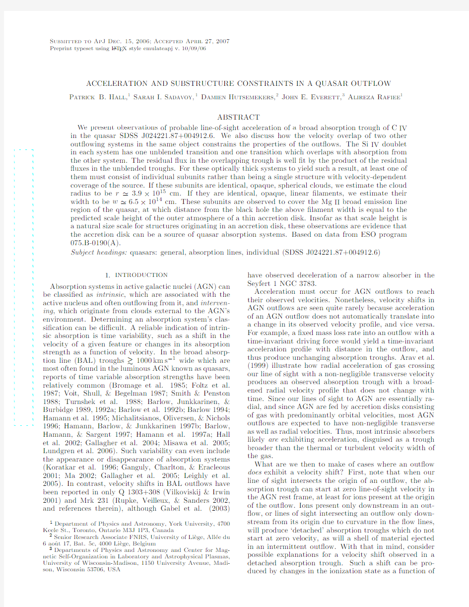
Submitted to ApJ Dec.15,2006;Accepted April 27,2007
Preprint typeset using L A T E X style emulateapj v.10/09/06
ACCELERATION AND SUBSTRUCTURE CONSTRAINTS IN A QUASAR OUTFLOW
Patrick B.Hall,1Sarah I.Sadavoy,1Damien Hutsemekers,2John E.Everett,3Alireza Rafiee 1
ABSTRACT
We present observations of probable line-of-sight acceleration of a broad absorption trough of C IV in the quasar SDSS J024221.87+004912.6.We also discuss how the velocity overlap of two other out?owing systems in the same object constrains the properties of the out?ows.The Si IV doublet in each system has one unblended transition and one transition which overlaps with absorption from the other system.The residual ?ux in the overlapping trough is well ?t by the product of the residual ?uxes in the unblended troughs.For these optically thick systems to yield such a result,at least one of them must consist of individual subunits rather than being a single structure with velocity-dependent coverage of the source.If these subunits are identical,opaque,spherical clouds,we estimate the cloud radius to be r ?3.9×1015cm.If they are identical,opaque,linear ?laments,we estimate their width to be w ?6.5×1014cm.These subunits are observed to cover the Mg II broad emission line region of the quasar,at which distance from the black hole the above ?lament width is equal to the predicted scale height of the outer atmosphere of a thin accretion disk.Insofar as that scale height is a natural size scale for structures originating in an accretion disk,these observations are evidence that the accretion disk can be a source of quasar absorption systems.Based on data from ESO program 075.B-0190(A).
Subject headings:quasars:general,absorption lines,individual (SDSS J024221.87+004912.6)
1.INTRODUCTION
Absorption systems in active galactic nuclei (AGN)can be classi?ed as intrinsic ,which are associated with the active nucleus and often out?owing from it,and interven-ing ,which originate from clouds external to the AGN’s environment.Determining an absorption system’s clas-si?cation can be di?cult.A reliable indication of intrin-sic absorption is time variability,such as a shift in the velocity of a given feature or changes in its absorption strength as a function of velocity.In the broad absorp-tion line (BAL)troughs 1000km s ?1wide which are most often found in the luminous AGN known as quasars,reports of time variable absorption strengths have been relatively common (Bromage et al.1985;Foltz et al.1987;Voit,Shull,&Begelman 1987;Smith &Penston 1988;Turnshek et al.1988;Barlow,Junkkarinen,&Burbidge 1989,1992a;Barlow et al.1992b;Barlow 1994;Hamann et al.1995;Michalitsianos,Oliversen,&Nichols 1996;Hamann,Barlow,&Junkkarinen 1997b;Barlow,Hamann,&Sargent 1997;Hamann et al.1997a;Hall et al.2002;Gallagher et al.2004;Misawa et al.2005;Lundgren et al.2006).Such variability can even include the appearance or disappearance of absorption systems (Koratkar et al.1996;Ganguly,Charlton,&Eracleous 2001;Ma 2002;Gallagher et al.2005;Leighly et al.2005).In contrast,velocity shifts in BAL out?ows have been reported in only Q 1303+308(Vilkoviskij &Irwin 2001)and Mrk 231(Rupke,Veilleux,&Sanders 2002,and references therein),although Gabel et al.(2003)
1
Department of Physics and Astronomy,York University,4700Keele St.,Toronto,Ontario M3J 1P3,Canada
2Senior Research Associate FNRS,University of Li`e ge,All′e e du 6ao?u t 17,Bat.5c,4000Li`e ge,Belgium
3Departments of Physics and Astronomy and Center for Mag-netic Self-Organization in Laboratory and Astrophysical Plasmas,University of Wisconsin-Madison,1150University Avenue,Madi-son,Wisconsin 53706,USA
have observed deceleration of a narrow absorber in the Seyfert 1NGC 3783.
Acceleration must occur for AGN out?ows to reach their observed velocities.Nonetheless,velocity shifts in AGN out?ows are seen quite rarely because acceleration of an AGN out?ow does not automatically translate into a change in its observed velocity pro?le,and vice versa.For example,a ?xed mass loss rate into an out?ow with a time-invariant driving force would yield a time-invariant acceleration pro?le with distance in the out?ow,and thus produce unchanging absorption troughs.Arav et al.(1999)illustrate how radial acceleration of gas crossing our line of sight with a non-negligible transverse velocity produces an observed absorption trough with a broad-ened radial velocity pro?le that does not change with time.Since our lines of sight to AGN are essentially ra-dial,and since AGN are fed by accretion disks consisting of gas with predominantly orbital velocities,most AGN out?ows are expected to have non-negligible transverse as well as radial velocities.Thus,most intrinsic absorbers likely are exhibiting acceleration,disguised as a trough broader than the thermal or turbulent velocity width of the gas.
What are we then to make of cases where an out?ow does exhibit a velocity shift?First,note that when our line of sight intersects the origin of an out?ow,the ab-sorption trough can start at zero line-of-sight velocity in the AGN rest frame,at least for ions present at the origin of the out?ow.Ions present only downstream in an out-?ow,or lines of sight intersecting an out?ow only down-stream from its origin due to curvature in the ?ow lines,will produce ‘detached’absorption troughs which do not start at zero velocity,as will a shell of material ejected in an intermittent out?ow.With that in mind,consider possible explanations for a velocity shift observed in a detached absorption trough.Such a shift can be pro-duced by changes in the ionization state as a function of
2Hall et al.
velocity in a?xed out?ow,by changes in the acceleration pro?le or geometry(or both)of such an out?ow due to changes in the driving force or mass loss rate,or by ac-tual line-of-sight acceleration of a shell of material from an intermittent out?ow.Observations of velocity shifts are therefore worthwhile because they may yield insights into speci?c scenarios for quasar absorbers.
Here we present multiple-epoch observations(§2)of a quasar in which a broad absorption line trough of C IV increased in out?ow velocity over1.4rest-frame years (§3).We also discuss how two overlapping out?ows in the same quasar provide constraints on the properties of those out?ows(§4).We end with our conclusions in§5.
2.OBSERVATIONS
The Sloan Digital Sky Survey(SDSS;York et al.2000) is using a drift-scanning camera(Gunn et al.1998)on a 2.5-m telescope(Gunn et al.2006)to image104deg2of sky on the SDSS ugriz AB magnitude system(Fukugita et al.1996;Hogg et al.2001;Smith et al.2002;Pier et al.2003;Ivezi′c et al.2004).Two multi-?ber,double spectrographs are being used to obtain resolution R~1850spectra covering?3800-9200?A for~106galaxies to r=17.8and~105quasars to i=19.1(i=20.2for z>3 candidates;Richards et al.2002).
The z em=2.062BAL quasar SDSS J024221.87+004912.6(Schneider et al.2002;Re-ichard et al.2003;Schneider et al.2005;Trump et al. 2006),hereafter referred to as SDSS J0242+0049,was observed spectroscopically three times by the SDSS(Ta-ble1).We selected it for high-resolution spectroscopic followup because of the possible presence of narrow absorption in excited-state Si II and C II at z=2.042.
A spectrum obtained with the ESO Very Large Tele-scope(VLT)Unit2(Kueyen)and Ultra-Violet Echelle Spectrograph(UVES;Dekker et al.2000)con?rms the presence of narrow,low-ionization absorption at that redshift,4analysis of which will be reported elsewhere. We observed SDSS J0242+0049with UVES on the VLT UT2on the nights of4-5September2005through a 1′′slit with2x2binning of the CCD,yielding R?40000. The weather ranged from clear to thin cirrus,with 0.8?1.0′′seeing.SDSS J0242+0049was observed for a total of5.75hours in two di?erent spectral settings,yield-ing coverage from3291-7521?A and7665-9300?A.Each exposure was reduced individually with optimum extrac-tion(Horne1986),including simultaneous background and sky subtraction.Telluric absorption lines were re-moved for the red settings using observations of telluric standard stars.A weighted co-addition of the three ex-posures of each spectral setting was performed with re-jection of cosmic rays and known CCD artifacts.Finally, all settings were rebinned to a vacuum heliocentric wave-length scale,scaled in intensity by their overlap regions, and merged into a single spectrum with a constant wave-length interval of0.08?A(Figure1).The SDSS spectra all share a common wavelength system with pixels equally spaced in velocity,and so for ease of comparison we cre-ated a version of the UVES spectrum binned to the those same wavelengths but not smoothed to the SDSS resolu-tion.
4The weak,narrow character of that absorption led to the classi-?cation of this object as a high-ionization BAL quasar by Reichard et al.(2003)and Trump et al.(2006)based on its SDSS spectrum.
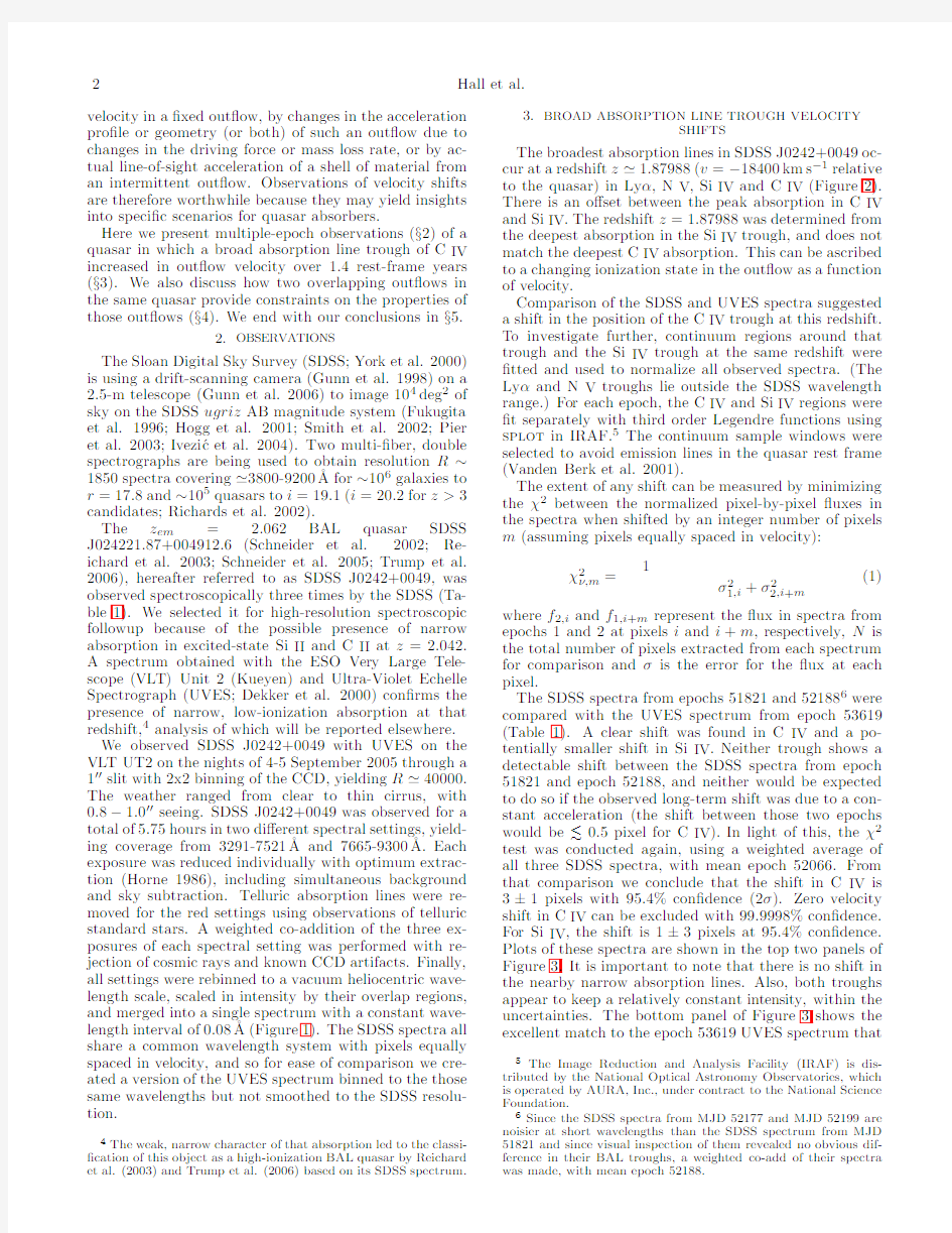
3.BROAD ABSORPTION LINE TROUGH VELOCITY
SHIFTS
The broadest absorption lines in SDSS J0242+0049oc-cur at a redshift z?1.87988(v=?18400km s?1relative to the quasar)in Lyα,N V,Si IV and C IV(Figure2). There is an o?set between the peak absorption in C IV and Si IV.The redshift z=1.87988was determined from the deepest absorption in the Si IV trough,and does not match the deepest C IV absorption.This can be ascribed to a changing ionization state in the out?ow as a function of velocity.
Comparison of the SDSS and UVES spectra suggested a shift in the position of the C IV trough at this redshift. To investigate further,continuum regions around that trough and the Si IV trough at the same redshift were ?tted and used to normalize all observed spectra.(The Lyαand N V troughs lie outside the SDSS wavelength range.)For each epoch,the C IV and Si IV regions were ?t separately with third order Legendre functions using splot in IRAF.5The continuum sample windows were selected to avoid emission lines in the quasar rest frame (Vanden Berk et al.2001).
The extent of any shift can be measured by minimizing theχ2between the normalized pixel-by-pixel?uxes in the spectra when shifted by an integer number of pixels m(assuming pixels equally spaced in velocity):
χ2ν,m=
1
σ21,i+σ22,i+m
(1)
where f2,i and f1,i+m represent the?ux in spectra from epochs1and2at pixels i and i+m,respectively,N is the total number of pixels extracted from each spectrum for comparison andσis the error for the?ux at each pixel.
The SDSS spectra from epochs51821and521886were compared with the UVES spectrum from epoch53619 (Table1).A clear shift was found in C IV and a po-tentially smaller shift in Si IV.Neither trough shows a detectable shift between the SDSS spectra from epoch 51821and epoch52188,and neither would be expected to do so if the observed long-term shift was due to a con-stant acceleration(the shift between those two epochs would be 0.5pixel for C IV).In light of this,theχ2 test was conducted again,using a weighted average of all three SDSS spectra,with mean epoch52066.From that comparison we conclude that the shift in C IV is 3±1pixels with95.4%con?dence(2σ).Zero velocity shift in C IV can be excluded with99.9998%con?dence. For Si IV,the shift is1±3pixels at95.4%con?dence. Plots of these spectra are shown in the top two panels of Figure3.It is important to note that there is no shift in the nearby narrow absorption lines.Also,both troughs appear to keep a relatively constant intensity,within the uncertainties.The bottom panel of Figure3shows the excellent match to the epoch53619UVES spectrum that 5The Image Reduction and Analysis Facility(IRAF)is dis-tributed by the National Optical Astronomy Observatories,which is operated by AURA,Inc.,under contract to the National Science Foundation.
6Since the SDSS spectra from MJD52177and MJD52199are noisier at short wavelengths than the SDSS spectrum from MJD 51821and since visual inspection of them revealed no obvious dif-ference in their BAL troughs,a weighted co-add of their spectra was made,with mean epoch52188.
Quasar Out?ow Constraints3
results when the epoch52066average SDSS spectrum is shifted by3pixels.
The middle panel of Figure3may suggest that the long-wavelength end of the C IV trough has a greater shift than the short-wavelength end.Splitting the C IV trough into two sections,we?nd thatχ2is minimized at a shift of2+2?1pixels for the short-wavelength end and a shift of4+1?2pixels for the long-wavelength edge,but that a uniform shift produces a marginally lower minimum overallχ2.Thus,while there is possible evidence for a nonuniform velocity shift of the C IV BAL trough,the current data are of insu?cient quality to prove its exis-tence.Many physical e?ects could produce a nonuniform shift(expansion of an overpressured,accelerated shell of gas from an intermittent out?ow,to give one example).
A shift of one SDSS pixel corresponds to a velocity shift of69km s?1in the observed frame or22.5km s?1in the quasar rest frame(z=2.062).A shift of3±1SDSS pixels(2σ)over a rest-frame time span of1.39years thus gives an acceleration of a=0.154±0.025cm s?2,where the error is1σ.Previously claimed accelerations for BAL troughs are much lower than that,at a=0.035±0.016 cm s?2over5.5rest-frame years in Q1303+308(Vilko-viskij&Irwin2001)and a=0.08±0.03cm s?2over 12rest-frame years for Mrk231(Rupke et al.2002). Our observation is more similar to that of Gabel et al. (2003),who determined the deceleration of C IV,N V and Si IV in a narrow absorption system in a Seyfert galaxy and found(for C IV)relatively large values of a=?0.25±0.05cm s?2and a=?0.10±0.03cm s?2 over0.75and1.1rest-frame years,respectively.All of those observations involved much narrower troughs than is the case in SDSS J0242+0049.Also,the1σrela-tive uncertainty associated with the acceleration of SDSS J0242+0049is lower than the previous BAL measure-ments.These factors make SDSS J0242+0049a robust case for line-of-sight acceleration of a true BAL trough. Still,it should be kept in mind that all these accelerations are much smaller than the a?100cm s?2predicted for the main acceleration phase of a disk wind in the model of Murray et al.(1995).
Furthermore,BAL troughs can vary for several rea-sons.These include acceleration or deceleration along the line of sight of some or all of the absorbing gas,a change in the ionization state of some or all of the gas, or a change in C(v)—the covering factor of the gas as a function of the line-of-sight velocity—due to the move-ment of gas into or out of our line of sight,for example due to a change in?ow geometry(see the introduction and§3.3of Gabel et al.2003).In many cases of vari-ability all of the above origins are possible,but there are cases where acceleration is very unlikely to be the cause(see below).Because of this,to be conservative we cannot assume that BAL trough variability is due to acceleration even though acceleration could be the cause of much of the observed variability.
Fig.2of Barlow et al.(1989)and Fig.2of Barlow et al.(1992b)are cases where observed time variabil-ity of BAL troughs is almost certainly due to a change in the column densities of an ion at certain velocities (whether due to a changing ionization or to bulk motion into the line of sight),not due to a given ionic column density changing its velocity.More ambiguous cases are illustrated by C IV in Q1246?057(Fig.3of Smith& Penston1988)and Si IV in Q1413+117(Fig.15of Turn-shek et al.1988).In both of those cases,a second-epoch spectrum shows more absorption at the short-wavelength edge of the trough in question.That could be because gas at lower out?ow velocities in the trough was acceler-ated to higher velocities.Yet in both cases,the trough away from the short-wavelength edge is unchanged be-tween the two epochs.If acceleration was the cause of the variability,a reduction in covering factor or optical depth,or both,might be expected at the lower velocities where the gas originated.No reduction is seen,arguing against the line-of-sight acceleration hypothesis for these cases of trough variability.
While every case for acceleration in a BAL trough will be ambiguous at some level,comparing the variability we report in SDSS J0242+0049to previous cases leads us to believe that ours is the least ambiguous case seen to date of acceleration in a true BAL trough( 1000km s?1 wide).Monitoring the future behavior of the z=1.87988 absorption in this quasar would be very worthwhile,to see if the acceleration was temporary,is constant,in-creasing,or decreasing,or varies stochastically.The lat-ter might occur if the velocity shift is due to a variable ?ow geometry or to ionization variations as a function of velocity caused by a?uctuating ionizing luminosity.(Re-call from Figure2that this system shows some evidence for ionization strati?cation with velocity,in the form of an o?set between the velocities of the peak Si IV and C IV absorption.)As this quasar is located in the equatorial stripe of the SDSS,which has been repeatedly imaged over the past7years,it should eventually be possible to search for a correlation between its ultraviolet luminosity and the acceleration of this system.(From the spectra alone,there appears to be a5-10%increase in the lumi-nosity of the object over the time spanned by the three SDSS spectra,but no information is available on longer timescales since the UVES spectrum is not spectropho-tometrically calibrated.)BAL trough velocity shifts are also expected if BAL quasars are a short-lived phase dur-ing which material is expelled from the nuclear region (Voit,Weymann,&Korista1993).In such a model the accelerating trough in SDSS J0242+0049could be inter-preted as gas unusually close to the quasar,currently experiencing an unusually large radiative acceleration.
4.OVERLAPPING SI IV TROUGHS
There is a possible case of line-locking involving Si IV in SDSS J0242+0049.Stable line-locking in a given dou-blet occurs when two conditions are met.First,the ve-locity separation between two absorption systems at dif-ferent redshifts must be very nearly equal to the velocity separation of the two lines of a doublet seen in both sys-tems(Braun&Milgrom1989).Second,the reduction in line-driven acceleration of the shadowed system due to the reduced incident?ux in one component of the dou-blet must result in its acceleration being the same as that of the shadowing system.This latter condition may be di?cult to meet in AGN out?ows,where many lines con-tribute to the radiative acceleration and there may also be substantial non-radiative acceleration.Nonetheless, some spectacular examples of apparent line-locking in AGN do suggest that it can in fact occur(e.g.,Srianand et al.2002),even if only rarely.
4Hall et al.
As shown in Figure4,in SDSS J0242+0049there is narrow Si IV absorption at z=2.0476(hereafter system A′)and a broad Si IV trough centered at about z=2.042 (hereafter system A).Si IV line-locking of a third absorp-tion system to system A′or A would result in absorption 1931km s?1shortward of those redshifts,at z=2.0280 or z=2.02245respectively.What is observed in the spectrum,however,is broad absorption in between the expected redshifts,centered at z=2.0254(hereafter sys-tem B).Both systems are observed in other transitions as well,with system B having more absorption in N V and C IV but less in S IV and Mg II.
In this section we consider?rst the optical depths and covering factors of these overlapping systems,with in-triguing results.We then consider whether they could be line-locked or in the process of becoming line-locked.
4.1.Si IV Trough Optical Depths and Covering Factors It is useful to determine if the Si IV troughs un-der consideration are optically thick or not.Figure5 shows the absorption pro?les in velocity space relative to z=2.0476or to the corresponding line-locked red-shift of z=2.0280.System A+A′,seen unblended in the bottom panel,is free from contamination in the blended trough(middle panel)at?900 For an unblended doublet,at each velocity v the nor-malized residual intensities I1and I2(in the stronger and weaker lines,respectively)can be related to the optical depth in the stronger transitionτand the fraction of the emitting source covered by the absorber along our line of sight,the covering factor C(e.g.,Hall et al.2003): I1(v)=1?C v(1?e?τv)(2) I2(v)=1?C v(1?e?Rτv)(3) where R measures the relative optical depths of the lines. For the Si IVλλ1393,1402doublet,R=0.5.In each ab-sorption system we have only one unblended component, but it can still be used to model the other component. (For comparison,the two unblended troughs are over-plotted on the blended trough in the top panel of Fig-ure6.) First we test whether system B can be optically thin, with C v=https://www.doczj.com/doc/8e6558156.html,ing this assumption and equations2and 3,the optical depthτv(λ1402,B)was calculated from the observed trough of Si IVλ1393in system B.The blended trough pro?le in this model should be exp[?τv(λ1402,B)] times the pro?le of Si IVλ1393in system A+A′.(The latter pro?le is taken as identical to theλ1402trough pro-?le at z=2.0476since system A+A′is optically thick.) The resulting model blended-trough pro?le is compared to the observed blended-trough pro?le in the second panel of Figure6.Optically thin absorption from sys-tem B falls short of explaining the depth of the blended trough. Next we test whether system B can be extremely op-tically thick,so that the depth of its absorption is deter-mined only by C v.In this case,we have two absorption systems absorbing at each v,but with di?erent C v.The total absorption is determined by C v,blended,which de-pends on what parts of the emitting source(s)are covered by neither absorption system,by just one,or by both. That is,the total absorption depends on the extent to which the two systems overlap transverse to our line of sight and cover the same parts of the source.We can rule out the limit of minimum overlap,which yields maximum coverage of the source:C v,blended=min(C A+C B,1).In that case C A+C B>1at all v,but we do not observed C v,blended=1at all v.Another limiting case is maxi-mum overlap of the absorption systems,which minimu-mizes the source coverage:C v,blended=max(C A,C B). The results of that model are shown in the third panel of Figure6.It is not an improvement over the opti-cally thin model.However,at almost all velocities the maximum-overlap model has more residual?ux than seen in the data,while the minimum-overlap model has less. Thus,overlap in C v which is less than the maximum possible by a velocity-dependent amount can explain the data.Such spatially-distinct,velocity-dependent partial covering has been seen before in other quasars(see the Appendix to Hall et al.2003). The last case we consider is one where each covering fraction describes the fractional coverage of the other ab-sorption system as well as of the continuum source,so that I v,blended=I A I B and C v,blended=C A+C B?C A C B (this is case3of Rupke et al.2005).The results of this model are shown in the bottom panel of Figure6,again assuming A and B are both very optically thick.The model reproduces the data reasonably well at almost all velocities,and much more closely overall than the other models considered. The good?t of this model implies that the absorption in one or both of the systems is produced by many small subunits scattered all over the continuum source from our point of view.In that case,the amount of light transmit-ted through both systems will naturally be I A(v)×I B(v) at every velocity v(Figure7).Deviations will only occur due to statistical?uctuations,which will be greater the fewer subunits there are.It is more di?cult,though still possible,to explain the observations using two‘mono-lithic’systems;that is,systems in which absorption from the ion in question arises in a single structure along our line of sight spanning the range of velocities seen in the trough,but with physical coverage of the source which varies with velocity(e.g.,Figure10of Arav et al.1999). Two monolithic?ows with unblended residual intensi-ties I A(v)and I B(v)can produce any blended residual intensity from0to min(I A(v),I B(v))essentially indepen-dently at each velocity v(Figure7).Thus,two mono-lithic?ows can explain the observations,but only if they just happen to overlap as a function of velocity in such a way as to mimic the overlap of two systems of clouds. Such an explanation is rather contrived,and we conclude instead that many small subunits exist in one or both absorption systems.This conclusion should of course be tested with observations of additional overlapping ab- Quasar Out?ow Constraints5 sorption systems in other quasars,to ensure this case is not a?uke. Note that we have not considered the e?ects of di?er- ent covering factors for the continuum source and broad emission line region.As seen in Figure4,line emission is a10%e?ect at best,and is not a factor at all in the Si IVλ1393trough of system B. 4.1.1.Constraints on the Out?ow Subunits The results above suggest that the absorbers A and B are composed of a number of optically thick subunits. We now discuss what we can infer about the parameters of these subunits,in the limit that each subunit is so optically thick it can be treated as opaque. Assume that absorber A’s residual intensity at some velocity,I A(v),is created by N A subunits intercepting our line of sight,and similarly for absorber B.When the two absorbers overlap along the line of sight,there will be N=N A+N B subunits along the line of sight.The average transmitted?ux i in this case will be= (1?p)N,where p is the average fraction of the quasar’s emission covered by an individual subunit. If an average N over all velocities is well de?ned,the pixel-to-pixel variations around the average value will be distributed with varianceσ2=σ2I+σ2i,whereσI is the instrumental error andσi is given by σ2i=σ2intrinsic+(1?p)2N N2σ2p 2(σ2I+σ2i) .(6) Each pixel has a di?erentσi which depends on the adopted a.To choose the best model,we?nd the value of a that maximizes the likelihood of the observations: L= k P(I k±σI k|i k±σi k).Note that a systematic er-ror in I(e.g.,due to a continuum estimate which is too high or too low)will yield a systematic error in a. We use the velocity range?700 To convert these to physical sizes,we model the quasar’s emission as being from a Shakura&Sunyaev (1973)accretion disk with viscosity parameterα=0.1 radiating at the Eddington limit.(We discuss the is-sue of coverage of the quasar’s broad emission line re-gion at the end of the section.)For this quasar we estimate M BH=6.2×10⁸M⊙from the second mo-ment of its Mg II emission line and its3000?A con-tinuum luminosity,using the methods of Ra?ee et al. (2007,in preparation).For those parameters,99%of the continuum emission at rest-frame1400?A comes from r<150R Sch,where R Sch=2GM BH/c2=1.8×1014cm is the Schwarzschild radius of the black hole.Since the relative sizes derived above were referenced to a square, not a circle,we adopt the square that has the same area as a circle with radius150R Sch,which has sides of length l=4.8×1016cm.Thus,we?nd a best-?t?lament width of w=6.5×1014cm,with a4σrange of6.7×1013 These sizes,small on astronomical scales,suggest an origin for the subunits in the accretion disk for either geometry.A plausible length scale for structures origi-nating in an accretion disk is the scale height h of its at-mosphere(Equation2.28of Shakura&Sunyaev1973).7 7If the accretion disk has a strong magnetic?eld,the pressure scale height may be a less plausible characteristic length.Numer- 6Hall et al. At large radii,h?3R3kT s/4GM BH m p z0where R is the distance from the black hole,T s is the disk surface temperature and z0is the disk half-thickness.(Though not obvious from the above,h We have outlined a consistent picture wherein systems A and B,whether they consist of opaque?laments or clouds,are launched from the accretion disk exterior to the Mg II BELR with a subunit size comparable to the scale height of the accretion disk atmosphere at that ra-dius.As a system accelerates,its typical density will decrease and its typical ionization will increase,explain-ing the presence of high ionization species in?ows aris-ing from a low-ionization emission-line region.When the systems cross our line of sight,they have line-of-sight velocities of v los=?2000km s?1for system A and v los=?3600km s?1for system B.For System A,|v los| is comparable to the v orbital=2900km s?1expected at its inferred launch radius of5500R Sch.For System B, |v los|is larger than the v orbital=1400km s?1expected at its inferred launch radius of25000R Sch.The spheri-cal cloud dispersal time would be of order~110years for T~104K,so the subunits will not disperse on their own between launch and crossing our line of sight.However, partial shadowing of a subunit will produce di?erential radiative acceleration of the subunit.Substantial radia-tive acceleration could thus shorten the subunit lifetimes considerably. One potential complication is that the observed pro?le of the overlapping trough deviates from the multiplica-ical simulations of accretion disks do not yet conclusively show if another characteristic scale is produced by magnetohydrodynamic turbulence(Armitage2004).tive prediction(Figure6,bottom panel)in a manner that is not random on velocity scales larger than~10km s?1. However,deviations on such scales should be random if, as expected,the individual subunits have velocity dis-persions of that order.Instead,the deviations seem to be coherent on~100km s?1scales.It may be that the subunits do have velocity widths of that order due to microturbulence(Bottor?et al.2000).Another possi-ble explanation is that the out?ow consists of?laments wherein the material is accelerated so that its line-of-sight velocity increases by~100km s?1as it crosses the line of sight(e.g.,Arav et al.1999).Deviations from the expected pro?le should then persist for~100km s?1 instead of~10km s?1.As compared to a model without line-of-sight acceleration,there could be the same aver-age number of?laments,but the number would change more slowly with velocity(although other e?ects,such as?laments not being exactly parallel,can a?ect that as well).Observations of additional overlapping systems would be useful for investigating this issue. We note that Goodman(2003)have shown that thin accretion disks without winds will be unstable to self-gravity beyond r Q=1?2740(108αl2E/M BH)2/9R Sch where l E is the Eddington ratio;using the parame-ters adopted herein,SDSS J0242+0049has r Q=1?1100R Sch.However,removal of angular momentum by a disk wind might help stabilize a thin disk(§4.3of Goodman2003),and there is reason to believe such a process operates in AGN.Reverberation mapping places the BELRs of many AGN at r>r Q=1,and there is ev-idence that BELRs are?attened(Vestergaard,Wilkes, &Barthel2000;Smith et al.2005;Aars et al.2005)as expected if they are located at the bases of accretion disk winds(Murray et al.1995).Furthermore,quasar spec-tral energy distributions are consistent with marginally gravitationally stable disks extending out to~105R Sch (Sirko&Goodman2003). Lastly,we note that there is no contradiction in us-ing the continuum source size to derive the scale size of the subunits for an out?ow the size of the BELR.This is because the continuum source has a surface bright-ness?2100times that of the BELR.That number is the ratio of the continuum?ux near1400?A in SDSS J0242+0049to the Si IV/O IV]?ux,which we take to be?9,times the ratio of the areas of the Si IV/O IV] BELR and the1400?A continuum source.8If N subunits of the absorber each cover a fractional area a of the con-tinuum source,Nx subunits of the absorber will each cover a fractional area a/x of the BELR.For large N and small a the residual intensity of each region is equal, i=(1?a)N?(1?a/x)Nx,but the variance on i from the BELR will be a factor?0.1/x smaller than the vari-ance on i from the continuum source.Thus,an absorber covering both the continuum source and BELR will have essentially the same residual intensity i and varianceσ2i (used to derive the absorber size constraints via Equation 6)as an absorber covering only the continuum source. 8The size of the Si IV/O IV]BELR has been measured in only three AGN(Peterson et al.2004).On average,it is comparable in size to the C IV BELR.We therefore use the relationship between Lλ(1350?A)and R BELR,CIV given by Peterson et al.(2006)to derive R BELR,SiIV=4.1×1017cm for SDSS J0242+0049. Quasar Out?ow Constraints7 4.2.Possible Si IV Line-Locking We now return to the issue of whether systems A+A′and B can be line-locked.Line-locking occurs when the reduction in line-driving?ux caused by the shadow of one system decelerates the other,shadowed system so that two systems end up with the same acceleration(which may be nonzero).The two systems thereafter maintain a constant velocity separation that keeps one system shad-owed(Braun&Milgrom1989).(However,there is some debate in the literature as to whether line-driven winds are unstable to the growth of shocks(Owocki,Castor,& Rybicki1988;Pereyra et al.2004).If shocks can develop, they could accelerate the wind out of an otherwise stable line-locking con?guration.)For line-locking to occur in an accelerating?ow,there are two possibilities.System B could have appeared along a sightline linking the con-tinuum source and system A+A′at2.0280 The latter scenario can be ruled out because the great-est deceleration of system A+A′would have occurred be-fore it reached z=2.0476,when it was shadowed by the deepest part of system B.Instead,the deepest part of system B is observed to be shadowed by the shallowest part of system A.If line-locking was going to occur in this scenario it would have had to set in when the shad-owing was greatest(or earlier than that,if less than full shadowing produced su?cient deceleration).If it did not happen then,it will not happen with the observed,lesser amount of shadowing. The former scenario of an accelerating system B which has ended up line-locked is plausible.The observed shad-owing as a function of velocity could in principle have halted system B. One requirement of this former scenario,however,is that the narrow absorption at z=2.0476(system A′) should not be associated with system A,the broad ab-sorption immediately shortwards of it.If they were asso-ciated,then some of the gas in system B at?350 The optically thickest part of system A is likely at ?650 Finally,note that the Si IV pro?les in SDSS J0242+0049are intriguingly similar to some of the poten-tially line-locked N V pro?les seen in RX J1230.8+0115 (Ganguly et al.2003).The z=0.1058system in that object has a pro?le similar to that of system A+A′(strongest absorption at both ends of the pro?le),and its z=0.1093system is similar to that of system B(opti-cally thick,with the strongest absorption in the middle of the pro?le,at a velocity corresponding to the weak-est absorption in the other system).Both systems have only about half the velocity widths of those in SDSS J0242+0049,however,and the relative velocities of the two systems are reversed—the weaker,single-peaked absorption pro?le has the lower out?ow velocity.It is also worth noting that the Lyαabsorption pro?le in each object appears to share the same covering factor as the species discussed above,while at least one moderately higher-ionization species in each object(N V here,and O VI in RX J1230.8+0115)has a larger covering factor which yields nearly black absorption troughs.Whether these similarities are just coincidences will require data on more candidate line-locking systems.(The line-locked systems in Q1511+091studied by Srianand et al.(2002) are much more complex,but do not seem to include any pro?les similar to those in SDSS J0242+0049.) 5.CONCLUSIONS We?nd that the C IV BAL trough at z=1.87988in the spectrum of SDSS J0242+0049(v=?18400km s?1 relative to the quasar’s rest frame)has likely undergone an acceleration of a=0.154±0.025cm s?2over a period of1.39rest-frame years.This is the largest acceleration yet reported in a BAL trough≥1000km s?1wide. We also derive constraints on the out?ow properties of two absorption systems,overlapping and possibly line-locked in Si IV,at z=2.0420and z=2.0254(v=?2000 km s?1and v=?3600km s?1relative to the quasar,re-spectively).The overlapping trough in common to both systems indicates that at least one of the systems must consist of individual subunits.This contrasts with re-sults strongly suggesting that the BELR itself consists of a smooth?ow,rather than a clumped one(Laor et al. 2006),but agrees with results for a narrow intrinsic ab-sorber in the gravitational lens RXS J1131?1231(Sluse et al.2007). Assuming identical,opaque subunits,our data are con-sistent with spherical clouds of radius r?3.9×1015cm or linear?laments of width w?6.5×1014cm.These subunits must be located at or beyond the Mg II broad emission line region.At that distance,the above?la-ment width is equal to the predicted scale height of the outer atmosphere of a thin accretion disk.Insofar as that 8Hall et al. is a natural length scale for structures originating in an accretion disk,these observations are evidence that the accretion disk is the source of the absorption systems.It would be useful to obtain high-resolution spectra of additional cases of distinct but overlapping intrinsic ab-sorption troughs in quasar spectra to determine if this case is representative.If so,it would also be worth ex-tending this work’s analytic study of the implications of the residual intensity variance to numerical studies in-cluding a realistic quasar geometry,a range in absorber sizes and optical depths,etc. We thank N.Murray for discussions,and the referee for helpful comments.P.B.H.is supported by NSERC,and S.I.S.was supported by an NSERC Undergrad-uate Summer Research Assistantship.The SDSS and SDSS-II (https://www.doczj.com/doc/8e6558156.html,/)are funded by the Al-fred P.Sloan Foundation,the Participating Institutions,the National Science Foundation,the U.S.Department of Energy,NASA,the Japanese Monbukagakusho,the Max Planck Society,and the Higher Education Funding Council for England,and managed by the Astrophysical Research Consortium for the Participating Institutions:American Museum of Natural History,Astrophysical In-stitute Potsdam,University of Basel,Cambridge Uni-versity,Case Western Reserve University,University of Chicago,Drexel University,Fermilab,the Institute for Advanced Study,the Japan Participation Group,Johns Hopkins University,the Joint Institute for Nuclear As-trophysics,the Kavli Institute for Particle Astrophysics and Cosmology,the Korean Scientist Group,the Chi-nese Academy of Sciences,Los Alamos National Labora-tory,the Max-Planck-Institute for Astronomy,the Max-Planck-Institute for Astrophysics,New Mexico State University,Ohio State University,University of Pitts-burgh,University of Portsmouth,Princeton University,the United States Naval Observatory,and the University of Washington. APPENDIX Consider the case of an absorber consisting of opaque subunits of a uniform shape.Suppose our line of sight to a quasar’s emitting regions is intercepted by N of these subunits,randomly distributed transverse to the line of sight.Then the scatter possible in the covering fraction at ?xed N due to the random overlap (or lack thereof)of the subunits with each other will depend on the shape of the subunits.To obtain expressions for this variance,we approximate the quasar’s emitting regions as a square of uniform surface brightness on the plane of the sky.We do this solely because expressions for the variance have been derived for the case of the unit square covered by two relevant subunit geometries:circles of area a and ?laments of unit length and width a .We take the ?rst case to represent a true cloud model,and the second to represent a magnetically con?ned ‘?lament’model. The case of the unit square randomly overlapped by ?laments parallel to each other and to two sides of the square,and of unit length and width a ,is treated by Robbins (1944).The unit square is de?ned as the set of points {0≤x ≤1;0≤y ≤1}.The ?laments that overlap the square are centered at y =0.5and distributed randomly in x over ?a 2.Because of edge e?ects,the average area covered by a ?lament is p = a (N +1)p ? 2a 2[(1?p )N +2?(1?2p )N +2] a/πof the unit square.Again the average area uncovered by N circles is given by i =(1?p )N ,but in this case p =πr 2/(1+4r +πr 2).The variance in the fractional area covered can be derived from expressions given by Kendall &Moran (1963),yielding σ2 circles = 1+4r ?πr 23 r 3?8r 4 ? 1+4r 2r +q 2r a a Quasar Out?ow Constraints9 REFERENCES Aars,C.E.,Hough,D.H.,Yu,L.H.,Linick,J.P.,Beyer,P.J., Vermeulen,R.C.,&Readhead,A.C.S.2005,AJ,130,23 Arav,N.,Korista,K.T.,de Kool,M.,Junkkarinen,V.T.,& Begelman,M.C.1999,ApJ,516,27 Armitage,P.J.2004,Theory of Disk Accretion onto Supermassive Black Holes(ASSL Vol.308:Supermassive Black Holes in the Distant Universe),89 Barlow,T.,Hamann,F.,&Sargent,W.1997,in ASP Conf.Ser. 128:Mass Ejection from Active Galactic Nuclei,13 Barlow,T.,Junkkarinen,V.,&Burbidge,E.1989,ApJ,347,674 Barlow,T.,Junkkarinen,V.,&Burbidge,E.1992a,in American Astronomical Society Meeting,Vol.181,1106 Barlow,T.,Junkkarinen,V.,Burbidge,E.,Weymann,R.,Morris, S.,&Korista,K.1992b,ApJ,397,81 Barlow,T.A.1994,PASP,106,548 Bottor?,M.C.,Ferland,G.J.,Baldwin,J.,Korista,K.2000,ApJ, 542,644 Braun,E.&Milgrom,M.1989,ApJ,342,100 Bromage,G.,Boksenberg,A.,Clavel,J.,Elvius,A.,Penston,M., Perola,G.,Pettini,M.,Snijders,M.,et al.1985,MNRAS,215, 1 Dekker,H.,D’Odorico,S.,Kaufer,A.,Delabre,B.,&Kotzlowski, H.2000,in Proc.SPIE Vol.4008,Optical and IR Telescope Instrumentation and Detectors,ed.M.Iye&A.Moorwood,534 Foltz,C.B.,Weymann,R.J.,Morris,S.L.,&Turnshek,D.A. 1987,ApJ,317,450 Fukugita,M.,Ichikawa,T.,Gunn,J.E.,Doi,M.,Shimasaku,K., &Schneider,D.P.1996,AJ,111,1748 Gabel,J.R.,Crenshaw,D.M.,Kraemer,S.B.,Brandt,W.N., George,I.M.,Hamann,F.W.,Kaiser,M.E.,Kaspi,S.,et al. 2003,ApJ,595,120 Gallagher,S.C.,Brandt,W.N.,Wills,B.J.,Charlton,J.C., Chartas,G.,&Laor,A.2004,ApJ,603,425 Gallagher,S.C.,Schmidt,G.D.,Smith,P.S.,Brandt,W.N., Chartas,G.,Hylton,S.,Hines,D.C.,&Brotherton,M.S.2005, ApJ,633,71 Ganguly,R.,Charlton,J.C.,&Eracleous,M.2001,ApJ,556,L7 Ganguly,R.,Eracleous,M.,Charlton,J.C.,&Churchill,C.W. 1999,AJ,117,2594 Ganguly,R.,Masiero,J.,Charlton,J.C.,&Sembach,K.R.2003, ApJ,598,922 Goodman,J.2003,MNRAS,339,937 Gunn,J.,Siegmund,W.,Mannery,E.,Owen,R.,Hull,C.,Leger, R.,Carey,L.,Knapp,G.,et al.2006,AJ,131,2332 Gunn,J.E.,Carr,M.,Rockosi,C.,Sekiguchi,M.,Berry,K.,Elms, B.,de Haas,E.,Ivezi′c,ˇZ.,et al.1998,AJ,116,3040 Hall,P.B.,Anderson,S.,Strauss,M.,York,D.,Richards,G.,Fan, X.,Knapp,G.,Schneider,D.,et al.2002,ApJS,141,267 Hall,P.B.,Hutsem′e kers,D.,Anderson,S.F.,Brinkmann,J.,Fan, X.,Schneider,D.P.,&York,D.G.2003,ApJ,593,189 Hamann,F.,Barlow,T.,Cohen,R.,Junkkarinen,V.,&Burbidge, E.1997a,in Mass Ejection from Active Galactic Nuclei,ed.N. Arav,I.Shlosman,&R.Weymann(San Francisco:ASP),19 Hamann,F.,Barlow,T.,&Junkkarinen,V.1997b,ApJ,478,87 Hamann,F.,Barlow,T.A.,Beaver,E.A.,Burbidge,E.M.,Cohen, R.D.,Junkkarinen,V.,&Lyons,R.1995,ApJ,443,606 Hogg,D.,Finkbeiner,D.,Schlegel,D.,&Gunn,J.2001,AJ,122, 2129 Horne,K.1986,PASP,98,609 Ivezi′c,ˇZ.,Lupton,R.,Schlegel, D.,Boroski, B.,Adelman-McCarthy,J.,Yanny,B.,Kent,S.,Stoughton,C.,et al.2004, AN,325,583 Kendall,M.G.&Moran,P.A.P.1963,Geometrical Probability (New York:Hafner),112 Koratkar,A.,Goad,M.,O’Brien,P.,Salamanca,I.,Wanders,I., Axon,D.,Crenshaw,D.,Robinson,A.,et al.1996,ApJ,470, 378Laor,A.,Barth,A.,Ho,L.,&Filippenko,A.2006,ApJ,636,83 Leighly,K.M.,Casebeer,D.A.,Hamann,F.,&Grupe,D.2005, in Bulletin of the American Astronomical Society,1184 Ma,F.2002,MNRAS,335,L99 Michalitsianos,A.G.,Oliversen,R.J.,&Nichols,J.1996,ApJ, 461,593 Misawa,T.,Eracleous,M.,Charlton,J.C.,&Tajitsu,A.2005, ApJ,629,115 Murray,N.,Chiang,J.,Grossman,S.,&Voit,G.1995,ApJ,451, 498 Owocki,S.P.,Castor,J.I.,&Rybicki,G.B.1988,ApJ,335,914 Pereyra,N.A.,Owocki,S.P.,Hillier,D.J.,&Turnshek,D.A. 2004,ApJ,608,454 Peterson,B.,Bentz,M.,Desroches,L.-B.,Filippenko,A.,Ho,L., Kaspi,S.,Laor,A.,Maoz,D.,et al.2006,ApJ,641,638 Peterson,B.,Ferrarese,L.,Gilbert,K.,Kaspi,S.,Malkan,M., Maoz,D.,Merritt,D.,Netzer,H.,et al.2004,ApJ,613,682 Peterson, B.M.1997,Active Galactic Nuclei(Cambridge: Cambridge University Press),71–89 Pier,J.R.,Munn,J.A.,Hindsley,R.B.,Hennessy,G.S.,Kent, S.M.,Lupton,R.H.,&Ivezi′c,ˇZ.2003,AJ,125,1559 Reichard,T.,Richards,G.,Schneider, D.,Hall,P.,Tolea, A., Krolik,J.,Tsvetanov,Z.,Vanden Berk,D.,et al.2003,AJ,125, 1711 Richards,G.,Fan,X.,Newberg,H.,Strauss,M.,Vanden Berk,D., Schneider,D.,Yanny,B.,Boucher,A.,et al.2002,AJ,123,2945 Robbins,H.E.1944,Annals of Mathematical Statistics,15,70 Rupke,D.S.,Veilleux,S.,&Sanders,D.B.2002,ApJ,570,588—.2005,ApJS,160,87 Schneider,D.P.,Hall,P.B.,Richards,G.T.,Vanden Berk,D.E., Anderson,S.F.,Fan,X.,Jester,S.,Stoughton,C.,et al.2005, AJ,130,367 Schneider,D.P.,Richards,G.T.,Fan,X.,Hall,P.B.,Strauss, M.A.,Vanden Berk,D.E.,Gunn,J.E.,Newberg,H.J.,et al. 2002,AJ,123,567 Shakura,N.I.&Sunyaev,R.A.1973,A&A,24,337 Sirko,E.&Goodman,J.2003,MNRAS,341,501 Sluse,D.,Claeskens,J.-F.,Hutsem′e kers,D.,&Surdej,J.,A&A, in press(astro-ph/0703030) Smith,J.,Tucker, D.,Kent,S.,Richmond,M.,Fukugita,M., Ichikawa,T.,Ichikawa,S.,Jorgensen,A.,et al.2002,AJ,123, 2121 Smith,J.E.,Robinson,A.,Young,S.,Axon,D.J.,&Corbett, E.A.2005,MNRAS,359,846 Smith,L.J.&Penston,M.V.1988,MNRAS,235,551 Srianand,R.,Petitjean,P.,Ledoux, C.,&Hazard, C.2002, MNRAS,336,753 Trump,J.,Hall,P.,Reichard,T.,Richards,G.,Schneider, D., Vanden Berk,D.,Knapp,G.,Anderson,S.,et al.2006,ApJS, 165,1 Turnshek,D.A.,Grillmair,C.J.,Foltz,C.B.,&Weymann,R.J. 1988,ApJ,325,651 Vanden Berk,D.E.,Richards,G.T.,Bauer,A.,Strauss,M.A., Schneider,D.P.,Heckman,T.M.,York,D.G.,Hall,P.B.,et al.2001,AJ,122,549 Vestergaard,M.,Wilkes,B.J.,&Barthel,P.D.2000,ApJ,538, L103 Vilkoviskij,E.Y.&Irwin,M.J.2001,MNRAS,321,4 Voit,G.M.,Shull,J.M.,&Begelman,M.C.1987,ApJ,316,573 Voit,G.M.,Weymann,R.J.,&Korista,K.T.1993,ApJ,413,95 York, D.,Adelman,J.,Anderson,J.,Anderson,S.,Annis,J., Bahcall,N.,Bakken,J.,Barkhouser,R.,et al.2000,AJ,120, 1579 10Hall et al. TABLE1 SDSS J0242+0049Spectroscopic Observations and Inferences SDSS SDSS Epoch?t rest Si IV,C IV Shift Si IV,C IV Shift Source Plate Fiber in MJD(days)vs.MJD52188vs.MJD53619 SDSS(1)40857651821?800,01,4 SDSS(2)7073325217736—— SDSS(3)7066175219943——SDSS Avg.(2+3)——(52188)40—1,3 SDSS Avg.(1+2+3)——(52066)0—1,3 UVES——536195071,3— Note.—Epochs are given on the Modi?ed Julian Day(MJD)system.The rest-frame time interval?t rest is given relative to MJD52066.Velocity shifts of absorption lines are given in SDSS pixels(69km s?1);the C IV shift is the?rst number and the Si IV shift is the second number. TABLE2 SDSS J0242+0049Subunit Parameters Subunit Avg.Number Best-?t Relative Relative99.994%Best-?t Physical Physical99.994%Atmospheric Geometry of SubunitsˉN Width or Radius Con?dence range Width or Radius Con?dence range(cm)Scale Height Distance Filaments203±810.01350.0014?0.04306.5×1014cm6.7×1013?2.1×10159.9×1017cm=5500R Sch Spheres177±710.0810.029?0.1433.9×1015cm1.4×1015?6.9×10154.5×1018cm=25000R Sch Note.—The average number of subunitsˉN is the number of subunits responsible for absorption at each pixel,averaged over all pixels.The total number of subunits present depends on the unknown velocity width of each subunit.The atmospheric scale height distance is the distance from the black hole at which the accretion disk atmospheric scale height equals the best-?t width or radius of the subunit in question;see§4.1.R Sch refers to the Schwarzschild radius of a black hole with mass6.2×108M⊙. Fig.1.—VLT UT2+UVES spectrum of SDSS J0242+0049,smoothed by a1?A boxcar?lter. Quasar Out?ow Constraints11 Fig. 2.—UVES spectra of BAL troughs in SDSS J0242+0049vs.velocity(in km s?1)in the z=1.87988frame.Negative velocities indicate blueshifts and positive velocities indicate redshifts relative to that frame.Zero velocity corresponds to the long-wavelength members of doublets,and dashed vertical lines indicate all components of each transition.Contaminating narrow absorption lines are present near all troughs,but especially in those found shortward of the Lyαforest. Fig. 3.—Comparison of the z=1.87988C IV BAL in SDSS J0242+0049at the average SDSS epoch and the UVES epoch.Negative velocities indicate blueshifts and positive velocities redshifts,relative to z=1.87988.The solid line is a weighted average of all three SDSS spectra.The dashed line is the UVES spectrum binned into the same pixels as the SDSS spectra.Dotted vertical lines indicate the?tting regions used when conducting theχ2test.The top panel compares the unshifted spectra for the Si IV trough,and the middle panel the unshifted spectra for the C IV trough.The bottom panel compares the C IV troughs after shifting the average SDSS spectrum toward shorter wavelengths by3pixels. 12Hall et al. Fig.4.—Two broad,overlapping Si IV doublets in the unnormalized spectrum of SDSS J0242+0049.Line identi?cations and redshifts for the di?erent troughs are given on the?gure.There is also narrow Si IV absorption at z=2.0314which is not marked. Fig.5.—Velocity plot of Si IV absorption after normalization by a?t to the total spectrum(continuum and weak emission lines). Quasar Out?ow Constraints13 Fig.6.—Fits to the blended Si IV trough.The trough containing blended absorption from both redshift systems is shown as the solid line in all panels.The?ts are shown as lighter lines with total error bars that include the observed errors on the?ux in the blended trough, so that at each pixel the deviation between the actual trough and the?t can be directly compared to the total accompanying uncertainty. Top panel:all three observed Si IV troughs are overplotted.The dashed line shows the unblended troughλ1393trough,plotted in the z=2.0280frame.The dot-dashed line shows the unblended troughλ1402trough,plotted in the z=2.0476frame.Second panel:the ?t and errors shown are for an optically thin lower-redshift system.Third panel:the?t and errors shown are for an optically thick lower-redshift system with maximum overlap in covering factor with the optically thick higher-redshift system.Bottom panel:the?t and errors shown are for the case where each system’s covering fraction describes its fractional coverage of the other absorption system,so that the residual?ux from both optically thick troughs can be multiplied together to give the residual?ux in this blended trough. 14Hall et al. Fig.7.—An illustration of how observations of optically thick absorption systems overlapping in velocity space can constrain absorber substructure.Each square is a schematic depiction of a quasar’s emission region at the same wavelengthλ.The hatched zones are the areas of the emission region covered by an absorber.The leftmost column depicts absorption by system A only,which is assumed to produce a normalized residual intensity of I A(λ)=0.5at the wavelength shown.The value of I A(λ)is the same regardless of whether the absorption is due to a monolithic?ow(top row)or due to randomly placed subunits(bottom row),here shown as spheres in projection.Similarly, the second column from the left depicts absorption by system B only,which is also assumed to produce a normalized residual intensity of I B(λ)=0.5at the wavelength shown.When systems A and B overlap,monolithic?ows can produce any normalized residual intensity in the range0≤I A+B(λ)≤0.5(top row,right)depending on the speci?c areas covered by each?ow at that wavelengthλ.On the other hand,?ows consisting of many randomly placed subunits will naturally yield an average value of==0.25at every wavelengthλwhere the systems overlap(bottom row,right).Deviations from this average will occur due to statistical?uctuations, which will be smaller the more subunits there are.Measuring the deviations thus enables us to constrain the size and number of the subunits(see§4.1.1). 初三数学坐标与函数 1. 如图,方格纸上一圆经过(2,5),(-2,l),(2,-3),( 6,1)四点,则该圆的圆心的坐标为() A.(2,-1)B.(2,2)C.(2,1)D.(3,l) 2.已知M(3a-9,1-a)在第三象限,且它的坐标都是整数,则a等于() A.1 B.2 C.3 D.0 3.在平面直角坐标系中,点P(-2,1)关于原点的对称点在() A.第一象限;B.第M象限; C.第M象限;D.第四象限 4.如图,△ABC绕点C顺时针旋转90○后得到AA′、B′C′, 则A点的对应点A′点的坐标是() A.(-3,-2); B.(2,2); C.(3,0); D.(2,l) 5.点P(3,-4)关于y轴的对称点坐标为_______,它 关于x轴的对称点坐标为_______.它关于原点的对 称点坐标为_____. 6.李明、王超、张振家及学校的位置如图所示. ⑴学校在王超家的北偏东____度方向上,与王超家 大约_____米。 ⑵王超家在李明家____方向上,与李明家的距离大约是____米; ⑶张振家在学校____方向上,到学校的距离大约是______ 米. 7.东风商场文具部的某种毛笔每支售价25元,书法练习本每本售价5元.该商场为了促销制定了两种优惠方法,甲:买一支毛笔就赠送一本书法练习本;乙:按购买金额打九折付款.某书法兴趣小组欲购买这种毛笔10支,书法练习本x(x>10)本. (1)写出每种优惠办法实际付款金额y甲(元)、y乙(元)与x(本)之间的关系式;(2)对较购买同样多的书法练习本时,按哪种优惠方法付款更省钱? 8. 某居民小区按照分期付款的形式福利售房,政府给予一定的贴息,小明家购得一套现价为120000元的房子,购房时首期(第一年)付款30000元,从第二年起,以后每年应付房款为5000元与上一年剩余欠款利息的和,设剩余欠款年利率为0.4%. (1)若第x(x≥2)年小明家交付房款y元,求年付房款y(元)与x(年)的函数关系式;(2)将第三年,第十年应付房款填人下列表格中 9. 如图所示,在直角坐标系中,第一次将△OAB变换成△OA1B1;第二次将OA1B1变换 应用matlab求解约束优化问题 姓名:王铎 学号: 2007021271 班级:机械078 上交日期: 2010/7/2 完成日期: 2010/6/29 一.问题分析 f(x)=x1*x2*x3-x1^6+x2^3+x2*x3-x4^2 s.t x1-x2+3x2<=6 x1+45x2+x4=7 x2*x3*x4-50>=0 x2^2+x4^2=14 目标函数为多元约束函数,约束条件既有线性约束又有非线性约束所以应用fmincon函数来寻求优化,寻找函数最小值。由于非线性不等式约束不能用矩阵表示,要用程序表示,所以创建m文件其中写入非线性不等式约束及非线性等式约束,留作引用。 二.数学模型 F(x)为目标函数求最小值 x1 x2 x3 x4 为未知量 目标函数受约束于 x1-x2+3x2<=6 x1+45x2+x4=7 x2*x3*x4-50>=0 x2^2+x4^2=14 三.fmincon应用方法 这个函数的基本形式为 x = fmincon(fun,x0,A,b,Aeq,beq,lb,ub,nonlcon,options) 其中fun为你要求最小值的函数,可以单写一个文件设置函数,也可是m文件。 1.如果fun中有N个变量,如x y z, 或者是X1, X2,X3, 什么的,自己排个顺序,在fun中统一都是用x(1),x(2)....x(n) 表示的。 2. x0, 表示初始的猜测值,大小要与变量数目相同 3. A b 为线性不等约束,A*x <= b, A应为n*n阶矩阵。 4 Aeq beq为线性相等约束,Aeq*x = beq。 Aeq beq同上可求 5 lb ub为变量的上下边界,正负无穷用 -Inf和Inf表示, lb ub应为N阶数组 6 nonlcon 为非线性约束,可分为两部分,非线性不等约束 c,非线性相等约束,ceq 可按下面的例子设置 function [c,ceq] = nonlcon1(x) c = [] ceq = [] 7,最后是options,可以用OPTIMSET函数设置,具体可见OPTIMSET函数的帮助文件。 四.计算程序 一次函数表达式与坐标(讲义) 一、 知识点睛 1. 一次函数表达式 直线(函数图象) 坐标 点 2. 坐标系中处理问题的原则 (1)坐标转线段长、线段长转坐标; (2)作横平竖直的线. 二、 精讲精练 1. 若点M 在函数y =2x -1的图象上,则点M 的坐标可能是( ) A .(-1,0) B .(0,-l) C .(1,-1) D .(2,4) 2. 若直线y =2x +1经过点(m +2,1-m ),则m =______. 3. 一次函数y =-2x +3与x 轴交于点_____,与y 轴交于点_____. 4. 在一次函数2 1 21+=x y 的图象上,与y 轴距离等于1的点的坐标为 __________________. 5. 若点(3,-4)在正比例函数y =kx 的图象上,那么这个函数的解析式为( ) A .43y x = B .43y x =- C .34y x = D .3 4 y x =- 6. 若正比例函数的图象经过点(-1,2),则这个图象必经过点( ) A .(1,2) B .(-1,-2) C .(2,-1) D .(1,-2) 7. 已知某个一次函数的图象过点A (-2,0),B (0,4),求这个函数的表达式. 8. 已知某个一次函数的图象过点A (3,0),B (0,-2),求这个函数的表达式. 9. 如图,直线l 是一次函数y =kx +b 的图象,填空: (1)k =______,b =______; (2)当x =4时,y =______; (3)当y =2时,x =______. 10. 已知y 是x 的一次函数,下表给出了部分对应值,则m 的值是________. 11. 一次函数y=kx +3的图象经过点A (1,2),则其解析式为____________. 12. 若一次函数y=2x+b 的图象经过点A (-1,1),则b =______,该函数图象经过 点B (1,___)和点C (_____,0). 13. 若直线y =kx +b 平行于直线y =3x +4,且过点(1,-2),则将y =kx+b 向下平移3 个单位得到的直线是_____________. 14. 在同一平面直角坐标系中,若一次函数y =-x +3与y =3x -5的图象交于点M , 则点M 的坐标为( ) A .(-1,4) B .(-1,2) C .(2,-1) D .(2,1) 15. 直线y =2x+b 经过直线y=x -2与直线y =3x +4的交点,则b 的值为( ) A .-11 B .-1 C .1 D .6 16. 当b=______时,直线y =2x +b 与y =3x -4的交点在x 轴上. 17. 一次函数y =kx +3的图象与坐标轴的两个交点间的距离为5,则k 的值为 __________. 18. 直线y =3x -1与两坐标轴围成的三角形的面积为_________. 19. 已知直线y =kx +b 经过(5,0),且与坐标轴所围成的三角形的面积为20,则 该直线的表达式为______________________. 20. 点A ,B ,C ,D 的坐标如图所示,求直线AB 与直线CD 的交点E 的坐标. 21. 如图,已知直线l 1:y =2x +3,直线l 2:y =-x +5,直线l 1,l 2分别交 x 轴于B , C 两点,l 1,l 2相交于点A . (1)求A ,B ,C 三点坐标; (2)S △ABC =________. 平面直角坐标系与函数知识要点归纳 怎样确定自变量的取值范围 函数自变量的取值范围是使函数解析式有意义的自变量的所有可能取值,它是一个函数被确定的重要因素。求函数自变量的取值范围通常有以下七种方法: 一、整式型:当函数解析是用自变量的整式表示时,自变量的取值范围是一切实数。 例1. 求下列函数中自变量x 的取值范围:(1);(2) 5 3213-=x y )( 二、分式型:当函数解析式是用自变量的分式表示时,自变量的取值范围应使分母不为零。 例2. 函数中,自变量x 的取值范围是________。 三、偶次根式型(主要是二次根式): 当函数解析式是用自变量的二次根式表示时,自变量的取值应使被开方数非负。 例3. 函数中,自变量x 的取值范围是________。 四、零指数或负指数: 当函数解析式是用自变量的零指数或负指数表示时,自变量的取值应使零指数或负指数的底数不为零。 例4、函数y=3x +(2x-1)0+(-x +3)-2 五、综合型:当函数解析式中含有整式、分式、二次根式、零指数或负指数时,要综合考虑,取它们的公共部分。 的取值范围是中,自变量、函数例x x x x x y 20 )3(1)2(5-++---= 。 六、实际问题型:当函数解析式与实际问题挂钩时,自变量的取值范围应使解析式具有实际意义。 例6. 拖拉机的油箱里有油54升,使用时平均每小时耗油6升,求油箱中剩下的油y (升)与使用时间t (小时)之间的函数关系式及自变量t 的取值范围。 七、几何问题型:当函数解析式与几何问题挂钩时,自变量的取值范围应使解析式具有几何意义。 例7. 等腰三角形的周长为20,腰长为x ,底边长为y 。求y 与x 之间的函数关系式及自变量x 的取值范围。 图像与坐标专练 例1:一次函数y=ax+b 的图象L 1关于直线y=-x 轴对称的图象L 2的函数解析式是_____ 练习:如图,已知点P(2m-1,6m-5)在第一象限角平分线OC 上,一直角顶点P 在OC 上,角两边与x 轴y 轴分别交于A 点B 点。 (1)求点P 的坐标 (2)当∠APB 绕着P 点旋转时,OA+OB 的长是否发生变化?若变化,求出其变化范围;若不变,求其值 的坐标坐标是____A1则点1=AB 3= OA , A1落在点A 对折,点OB 沿OABC 将矩形如图图在直角坐标系中2,,已知:例 的解析式.AM ′处处,求直B 轴上的点x 恰好落在B 折叠叠,AM 沿ABM 若将△上的一点,OB 是M ,B 和点A 轴分别交于点y 轴、x 与练习:直线83 4+-=x y 的值 a 的面积面积相等ABC 与△ABP △使),2 1(a,P 有一点90=BAC 是等腰直角三角形,∠ABC 且△点在第一象限,C 两点,B 、A 轴分别交于y 轴x 1的的图的x 3 3-=y 函数3,在第二象限:例? + 的值值 a 面积积相等,求实ABP 与△ABC )若△3(的面积面 ABC )求△2(; m )画出直线1(,a)(1P 90=BAC 是等腰直角三角形,∠ABC 且△点在第一象限,C 两点,B 、A 轴分别交于y 轴x 1的的图的x 3 3- =y 函数为坐标系中一动点,,点练习:?+ 随堂练习: 1.如图,点A 的坐标为(-1,0),点B 在直线y=x(改为y=2x-4时又如何)上运动,当线段AB 最短时,点B 的坐标是? (1图)(2图) 2.直线AB : y=1/2 x+1 分别与x 轴、y 轴交于点A 、点B ;直线CD :y=x+b 分别与x 轴、y 轴交于点C 、点D .直线AB 与CD 相交于点P .已知S △A B D =4,则点P 的坐标是? 3.如图,正方形ABCD 的边长为4,点P 为正 方形边上一动点,若点P 从点A 出发沿A→D→C→B→A 匀速运动一周.设点P 走过的路程为x ,△ADP 的面积 为y ,则下列图象 能大致反映y 与x 的函数关系的是( ) A. B. C. D. 4.点A 坐标(5,0),直线y=x+b(b>=0)与y 轴交于点B ,连接AB ,角a=75度,则b 的值为_______ (4图) (5图) 5.已知OB 是一次函数y=2x 的图像,点A (0,2),在直线OB 上找一点C ,使得三角形ACO 为等腰三角形,求点C 的坐标。 用宏表函数与公式 1. 首先:点CTRL+F3打开定义名称,再在上面输入“纵当页”,在下面引用位置处输入: =IF(ISNA(MATCH(ROW(),GET.DOCUMENT(64))),1,MATCH(ROW(),GET.DOCUMENT(64))+1) 2.然后再继续添加第二个名称:“横当页”,在下面引用位置处输入: =IF(ISNA(MATCH(column(),GET.DOCUMENT(65))),1,MATCH(column(),GET.DOCUMENT(65))+1) 3.再输入“总页”;引用位置处输入:(在MSoffice2007不管有多少页,都只显示共有1页,不知为什么) =GET.DOCUMENT(50)+RAND()*0 4.最后再定义“页眉”,引用位置: ="第"&IF(横当页=1,纵当页,横当页+纵当页)&"页/共"&总页&"页" 5.在函数栏使用应用即可得到需要的页码。 另外一般情况下,一般的表册都要求每页25行数据,同时每页还需要设置相同的表头,虽然上面的方法可以在任意单元格内计算所在页面的页码,但是如果公式太多的话,计算特别慢。如果每页行数是固定的(比如25行)话,就可以采用下面的笨方法。 1、设置顶端标题行,“页面设置”→“工作表”→“顶端标题行”中输入“$1:$4”(第1行到第4行) 2、在工作表中数据输入完毕后,设置好各种格式,除表头外,保证每页是25行数据。 3、在需要设置该行所在页面的页码的单元格内输入如下公式: =INT((ROW()-ROWS(Print_Titles)-1)/25)+1 (公式里面的Print_Titles就是前面第1步所设置的顶端标题行区域。) 4、通过拖动或者复制的方法复制上面的公式,即可得到页码。 第十五讲 函数与坐标系 【学习目标】 1、复习平面直角坐标系的有关概念,明确点的位置与点的坐标之间的关系 2、复习函数的一般概念,以及用解析法表示简单的函数,会画函数的图像 3、进一步培养函数的思想以及数形结合的思想 【知识要点】 1、 平面直角坐标系的基本知识: ①直角坐标系的画法;②坐标系内各象限的编号顺序及各象限内点的坐标的符号 2、函数的定义,以及用解析法表示函数时要注意考虑自变量的取值必须使解析式有意义 3、函数的图象: (1)函数图象上的点的坐标都满足函数解析式,以满足函数解析式的自变量值和与它对应的函数值为坐标的点都在函数图象上. (2)知道函数的解析式,一般用描点法按下列步骤画出函数的图象: 列表.在自变量的取值范围内取一些值,算出对应的函数值,列成表. 描点.把自变量的值和与它相应的函数值分别作为横坐标与纵坐标,在坐标平面内描出相应的点. 连线.按照自变量由小到大的顺序、用平滑的曲线把所描各点连结起来. 【典型例题】 例1、点P (-1,-3)关于y 轴对称的点的坐标是_____________;关于x 轴的对称的点的坐标是 ____________;关于原点对称的点的坐标是____________。 例2、(1)若点P (a ,b )在第四象限,则点M (b -a ,a -b )在( ) A 、第一象限 B 、第二象限 C 、第三象限 D 、第四象限 (2)已知点P (a ,b ),a ·b >0,a +b <0,则点P 在( ) A 、第一象限 B 、第二象限 C 、第三象限 D 、第四象限 (3)已知点P (x ,y )的坐标满足方程|x +1|+y -2 =0,则点P 在( ) A 、第一象限 B 、第二象限 C 、第三象限 D 、第四象限 (4) 已知点A 233x x --,在第二象限,化简491232x x x +---=________ 例3、函数自变量的取值范围: (1)函数y =1x -1 中自变量x 的取值范围是 平面直角坐标系与函数 基础题目 一选择题 1.在平面直角坐标系中,点P(x2+2,-3)所在的象限是() A.第一象限B.第二象限C.第三象限D.第四象限 2.在平面直角坐标系的第二象限内有一点M,点M到x轴的距离为4,到y轴的距离为3,则点M的坐标是() A.(3,-4)B.(4,-3)C.(-4,3)D.(-3,4) 3.已知:如图,等边三角形OAB的边长为23边OA在x轴正半轴上,现将等边三角形OAB 绕点O逆时针旋转,每次旋转60°,则第2020次旋转结束后,等边三角形中心的坐标为()A.(3,1)B.(0,-1)C.(3-1) D.(0,-2) 4.如图,一个函数的图象由射线BA,线段BC,射线CD组成、其中点A(-2,2),B(1,3),C(2,1),D(6,5),则() A.当<2时,y随x的增大而增大 B.当x<2时,y随x的增大而减小 C.当x>2时,y随x的增大而增大 D.当x>2时,y随x的增大减小 5.(2020?河南模拟)如图,矩形ABCD的周长是28cm,且AB比BC长2cm.若点P从点A 出发,以1cm/s的速度沿A→D→C方向匀速运动,同时点Q从点A出发,以2cm/s的速度沿A→B→C方向匀速运动,当一个点到达点C时,另一个点也随之停止运动.若设运动时间为t(s),△APQ的面积为S(cm2),则S(cm2)与t(s)之间的函数图象大致是() 第3题图 第4题图 第5题图 A B C D 6.若点A (n ,m )在第四象限,则点B (m 2,-n )在( ) A.第四象限 B.第三象限 C.第二象限 D.第可以象限 二填空题 7.点P (m ,2)在第二象限内,则m 的值可以是__________.(写出一个即可) 8.已知点P (x ,y )位于第四象限,并且x ≤y+4(x ,y 为整数),写出一个符合条件的点P 的坐标:__________. 9.函数13 x y x -=-的自变量x 的取值范围是__________. 10中国象棋是中华民族的文化瑰宝,因趣味性强,深受大众喜爱.如图,若在象棋棋盘上建立平面直角坐标系,使“帅”位于点(0,-2),“马”位于点(4,-2),则“炮”位于点 __________. 11.如图,已知点A 1(1,1),将点A 1向上平移1个单位长度,再向右平移2个单位长度得 到点A 2;将点A 2向上平移2个单位长度,再向右平移4个单位长度得到点A 3;将点A 3向上平移4个单位长度,再向右平移8个单位长度得到点A 4,…按这个规律平移下去得到点A n (n 为正整数),则点A n 的坐标是__________. Excel常用函数公式大全 1、查找重复内容公式:=IF(COUNTIF(A:A,A2)>1,"重复","")。 2、用出生年月来计算年龄公式:=TRUNC((DAYS360(H6,"2009/8/30",FALSE))/360,0)。 3、从输入的18位身份证号的出生年月计算公式: =CONCATENATE(MID(E2,7,4),"/",MID(E2,11,2),"/",MID(E2,13,2))。 4、从输入的身份证号码内让系统自动提取性别,可以输入以下公式: =IF(LEN(C2)=15,IF(MOD(MID(C2,15,1),2)=1,"男","女"),IF(MOD(MID(C2,17,1),2)=1,"男","女"))公式内的“C2”代表的是输入身份证号码的单元格。 1、求和:=SUM(K2:K56) ——对K2到K56这一区域进行求和; 2、平均数:=AVERAGE(K2:K56) ——对K2 K56这一区域求平均数; 3、排名:=RANK(K2,K$2:K$56) ——对55名学生的成绩进行排名; 4、等级:=IF(K2>=85,"优",IF(K2>=74,"良",IF(K2>=60,"及格","不及格"))) 5、学期总评:=K2*0.3+M2*0.3+N2*0.4 ——假设K列、M列和N列分别存放着学生的“平时总评”、“期中”、“期末”三项成绩; 6、最高分:=MAX(K2:K56) ——求K2到K56区域(55名学生)的最高分; 7、最低分:=MIN(K2:K56) ——求K2到K56区域(55名学生)的最低分; 8、分数段人数统计: (1)=COUNTIF(K2:K56,"100") ——求K2到K56区域100分的人数;假设把结果存放于K57单元格; (2)=COUNTIF(K2:K56,">=95")-K57 ——求K2到K56区域95~99.5分的人数;假设把结果存放于K58单元格; (3)=COUNTIF(K2:K56,">=90")-SUM(K57:K58) ——求K2到K56区域90~94.5分的人数;假设把结果存放于K59单元格; (4)=COUNTIF(K2:K56,">=85")-SUM(K57:K59) ——求K2到K56区域85~89.5分的人数;假设把结果存放于K60单元格; 课题:函数的定义、平面直角坐标系 主备:朱贝课型:复习审核:九年级数学组 班级姓名学号 【学习目标】 1. 函数的相关概念及表示方法 2. 平面直角坐标系中,点坐标的表示和相关应用 【重点难点】 重点:函数的相关概念及表示方法,平面直角坐标系的应用难点:函数和坐标系的应用【知识梳理】 一、函数的概念及表示方法 1.在某一过程中可以取不同数值的量叫做___ _____ ,保持同一数值的量叫做。2.如果那么, y叫做x的函数,x叫做。 3.函数的三种表示方法是:、、。二、平面直角坐标系 1.点P(a,b),关于x轴对称点的坐标为 ________,关于y轴对称点的坐标为_________,关于原点的坐标为___ __;点P(a,b),到x轴的距离为;到y轴的距离为,到原点的距离为。x轴上的点A坐标为(a, ),y轴上的点B坐标为(,b)。 2.在平面直角坐标系中,线段AB‖x轴,A(a,b),B (c,d),则AB= ,b d;线段CD‖y轴,C(e,f)B (g,h),则CD= ,e g。 【课前练习】 1.已知点P(-2m,m-6) (1)当m=-1时,点P在第象限; (2)当点P在x轴上时,m= ; (3)当点P在第三象限时,m的取值范围是。 2.点M(4,0)到点(-1,0)距离是;点P(-5,12)到x轴的距离是,到y轴的距离是,到原点的距离是。 3.在平面直角坐标系中,线段AB‖x轴,点A(2,3),AB=5,则点B的坐标为。4.已知线段CD是由线段AB平移得到的,点A(﹣1,4)的对应点为C(4,7),则点B(﹣4, 5.边长为a的等边三角形,其面积S= ,其中常量是,变量是, 宏表函数 贡献者:zuazua日期:2010-11-18 阅读:2484 相关标签:et2010 > 公式 > 函数 > 宏表函数 EVALUATE 对以文字表示的一个公式或表达式求值,并返回结果 INDIRECT函数 贡献者:843211日期:2008-07-21 阅读:58024 相关标签:et2007 > 公式 > 函数 > 函数类型 > 查找与引用函数 > INDIRECT 返回由文本字符串指定的引用。此函数立即对引用进行计算,并显示其内容。当需要更改公 式中单元格的引用,而不更改公式本身,请使用函数INDIRECT。 语法 INDIRECT(ref_text,a1) Ref_text 为对单元格的引用,此单元格可以包含A1-样式的引用、R1C1-样式的引用、定 义为引用的名称或对文本字符串单元格的引用。如果ref_text 不是合法的单元格的引用, 函数INDIRECT 返回错误值#REF!。 ? 如果ref_text 是对另一个工作簿的引用(外部引用),则那个工作簿必须被打开。如果 源工作簿没有打开,函数INDIRECT 返回错误值#REF!。 A1 为一逻辑值,指明包含在单元格ref_text 中的引用的类型。 ? 如果a1 为TRUE 或省略,ref_text 被解释为A1-样式的引用。 ? 如果a1 为FALSE,ref_text 被解释为R1C1-样式的引用。 示例 如果您将示例复制到空白工作表中,可能会更易于理解该示例。 A B 1数据数据 2B2 1.333 3B345 4George10 5562 公式说明(结果) =INDIRECT($A$2)单元格A2中的引用值(1.333) =INDIRECT($A$3)单元格A3中的引用值(45) =INDIRECT($A$4)如果单元格B4有定义名“George”,则返回定义名的值(10) =INDIRECT("B"&$A$5)单元格A5中的引用值(62) 第十章约束条件下多变量函数 的寻优方法 ●将非线性规划→线性规划 ●将约束问题→无约束问题 ●将复杂问题→较简单问题 10.1约束极值问题的最优性条件 非线性规划:min f(X) h i(X)=0 (i=1,2,…,m) (10.1.1) g j(X)≥0 (j=1,2,…,l) 一、基本概念 1.起作用约束 设X(1)是问题(10.1.1)的可行点。对某g j(X)≥0而言: 或g j(X(1))=0:X(1)在该约束形成的可行域边界上。 该约束称为X(1)点的起作用约束。 或g j(X(1))>0:X(1)不在该约束形成的可行域边界上。 该约束称为X(1)点的不起作用约束。 X(1)点的起作用约束对X(1)点的微小摄动有某种限制作用。等式约束对所有可行点都是起作用约束。 () θcos ab b a =? 2.正则点 对问题(10.1.1),若可行点X (1)处,各起作用约束的梯度线性无关,则X (1)是约束条件的一个正则点。 3.可行方向(对约束函数而言) 用R 表示问题(10.1.1)的可行域。设X (1)是一个可行点。对某方向D 来说,若存在实数λ1>0,使对于任意λ(0<λ<λ1)均有X (1)+λD ∈R ,则称D 是点X (1)处的一个可行方向。 经推导可知,只要方向D 满足: ▽g j (X (1))T D>0 (j ∈J ) (10.1.3) 即可保证它是点X (1)的可行方向。J 是X (1)点起作用约束下标的集合。 在X (1)点,可行方向D 与各起作用约束的梯度方向的夹角为锐角 。 4.下降方向(对目标函数而言) 设X (1)是问题(10.1.1)的一个可行点。对X (1)的任一方向D 来说,若存在实数λ1>0,使对于任意λ(0<λ<λ1)均有f(X (1)+λD) 1.拆分单元格赋值 Sub 拆分填充() Dim x As Range For Each x In https://www.doczj.com/doc/8e6558156.html,edRange.Cells If x.MergeCells Then x.Select x.UnMerge Selection.Value = x.Value End If Next x End Sub 2.E xcel 宏按列拆分多个excel Sub Macro1() Dim wb As Workbook, arr, rng As Range, d As Object, k, t, sh As Worksheet, i& Set rng = Range("A1:f1") Application.ScreenUpdating = False Application.DisplayAlerts = False arr = Range("a1:a" & Range("b" & Cells.Rows.Count).End(xlUp).Row) Set d = CreateObject("scripting.dictionary") For i = 2 To UBound(arr) If Not d.Exists(arr(i, 1)) Then Set d(arr(i, 1)) = Cells(i, 1).Resize(1, 13) Else Set d(arr(i, 1)) = Union(d(arr(i, 1)), Cells(i, 1).Resize(1, 13)) End If Next k = d.Keys t = d.Items For i = 0 To d.Count - 1 Set wb = Workbooks.Add(xlWBATWorksheet) With wb.Sheets(1) rng.Copy .[A1] t(i).Copy .[A2] End With wb.SaveAs Filename:=ThisWorkbook.Path & "\" & k(i) & ".xlsx" wb.Close Next 函数的基础知识1 一.选择题(共9小题) 1.函数中,自变量x的取值范围是() A.x≠3 B.x≥3 C.x>3 D.x≤3 2.(2014?海南,第8题3分)如图,△ABC与△DEF关于y轴对称,已知A(﹣4,6),B(﹣6,2),E(2,1),则点D的坐标为() A.(﹣4,6)B.(4,6)C.(﹣2,1)D.(6,2) 3.(2014?黑龙江牡丹江, 第6题3分)如图,把ABC经过一定的变换得到△A′B′C′,如果△ABC上点P的坐标为(x,y),那么这个点在△A′B′C′中的对应点P′的坐标为() 第3题图 A.(﹣x,y﹣2)B.(﹣x,y+2)C.(﹣x+2,﹣y)D.(﹣x+2,y+2) 4.函数y=中,自变量x的取值范围是() A.x≠0 B.x≥2 C.x>2且x≠0 D.x≥2且x≠0 5.甲、乙两人以相同路线前往距离单位10km的培训中心参加学习.图中l甲、l乙分别表示甲、乙两人前往目的地所走的路程S(km)随时间t(分)变化的函数图象.以下说法:①乙比甲提前12分钟到达;②甲的平均速度为15千米/小时;③乙走了8km后遇到甲;④乙出发6分钟后追上甲.其中正确的有() A.4个B.3个C.2个D.1个 6.小明从家出发,外出散步,到一个公共阅报栏前看了一会报后,继续散步了一段时间,然后回家,如图描述了小明在散步过程汇总离家的距离s(米)与散步所用时间t(分)之间的函数关系,根据图象,下列信息错误的是() A.小明看报用时8分钟B.公共阅报栏距小明家200米 C.小明离家最远的距离为400米D.小明从出发到回家共用时16分钟 7.园林队在某公园进行绿化,中间休息了一段时间.已知绿化面积S(单位:平方米)与工作时间t(单位:小时)的函数关系的图象如图,则休息后园林队每小时绿化面积为() A.40平方米B.50平方米C.80平方米D.100平方米 8.已知,A、B两地相距120千米,甲骑自行车以20千米/时的速度由起点A前往终点B,乙骑摩托车以40千米/时的速度由起点B前往终点A.两人同时出发,各自到达终点后停止.设两人之间的距离为s(千米),甲行驶的时间为t(小时),则下图中正确反映s与t之间函数关系的是() A.B. 备用图 1、如图,△ABC内接于⊙O,AD⊥BC,OE⊥BC, OE= 1 2 BC.(1)求∠BAC的度数. (2)将△ACD沿AC折叠为△ACF,将△ABD沿AB折叠为△ABG,延长FC和GB相交于点H.求证: 四边形AFHG是正方形. (3)若BD=6,CD=4,求AD的长. 2.如图所示,平面直角坐标系中, 抛物线y=ax2+bx+c 经过 A(0,4)、B(-2,0)、C(6,0).过点A 作AD∥x轴交抛物线于点D,过点D作DE⊥x轴,垂足为点E.点M是四边形OADE的对角线的交点, 点F在y轴负半轴上,且F(0,-2). (1)求抛物线的解析式,并直接写出四边形OADE的形状; (2)当点P、Q从C、F两点同时出发,均以每秒1个长度单位的速度沿CB 、FA方向运动,点P 运动到O时P、Q两点同时停止运动.设运动的时间为t秒,在运动过程中,以P、Q、O、M四点为 顶点的四边形的面积为S,求出S与t之间的函数关系式,并写出自变量的取值范围; (3)在抛物线上是否存在点N,使以B、C、F、N为顶点的四边形是梯形?若存在,直接写出点N 的坐标;不存在,说明理由. 3.如图,已知抛物线y=x2+bx+c与x轴交于A、B两点(A点在B点左侧),与y轴交于点C (0,-3),对称轴是直线x=1,直线BC与抛物线的对称轴交于点D.⑴求抛物线的函数表达式; ⑵求直线BC的函数表达式;⑶点E为y轴上一动点,CE的垂直平分线交CE于点F,交抛物线 于P、Q两点,且点P在第三象限. ①当线段PQ= 3 4 AB时,求tan∠CED的值; ②当以点C、D、E为顶点的三角形是直角三角形时,请直接写出点P的坐标. 4、如图,在平面直角坐标系中,O是坐标原点,直线9 4 3 + - =x y与x轴,y轴分别交于B,C 两点,抛物线c bx x y+ + - =2 4 1 经过B,C两点,与x轴的另一个交点为点A,动点P从点A出 发沿AB以每秒3个单位长度的速度向点B运动,运动时间为t(0<t<5)秒. (1)求抛物线的解析式及点A的坐标; (2)以OC为直径的⊙O′与BC交于点M,当t为何值时,PM与⊙O′相切?请说明理由。 (3)在点P从点A出发的同时,动点Q从点B出发沿BC以每秒3个单位长度的速度向点C 运 动,动点N从点C出发沿CA以每秒 5 10 3 个单位长度的速度向点A运动,运动时间和点P相 同。 ①记△BPQ的面积为S,当t为何值时,S最大,最大值是多少? ②是否存在△NCQ为直角三角形的情形,若存在,求出相应的t值;若不存在,请说明理由. 一、填空和选择 1.(2009,达州)在平面直角坐标系中,设点P 到原点O 的距离为ρ,OP 与x 轴正方向的夹角为α,则用][α ρ,表示点P 的极坐标,显然,点P 的极坐标与它的坐标存在一一对应关系.例如:点P 的坐标为(1, 1),则其极坐标为[]?45,2.若点Q 的极坐标为[]?60,4,则点Q 的坐标为( ) A.()32,2 B.()32,2- C.(23,2) D.(2,2) 2、在坐标平面内,横、纵坐标都是整数的点叫做整点,若点P (2a +1,4a -15)是第四象限内的整点,则整数a = . 3.已知点A (x 1,y 1),点B (x 2,y 2),则线段AB 的中点坐标为??? ??++2,22121y y x x . 4、在平面直角坐标系中,已知线段AB 的两个端点分别是()()41A B --,,1,1,将线段AB 平移后得到线段A B '',若点A '的坐标为()22-,,则点B '的坐标为( ) A .()43, B .()34, C .()12--, D .()21--, 5. (2009仙桃)如图,把图①中的⊙A 经过平移得到⊙O (如图②),如果图①中⊙A 上一点P 的坐标为(m , n ),那么平移后在图②中的对应点P’的坐标为( ). A .(m +2,n +1) B .(m -2,n -1) C .(m -2,n +1) D .(m +2,n -1) 7、正方形ABCD 在坐标系中的位置如图所示,将正方形ABCD 绕D 点顺时针旋转90°后,B 点的坐标为( ) A .(4,0) B .(4,1) C .(-2,2) D .(3,1) 8.将点A (4,0)绕着原点O 顺时针方向旋转30°角到对应点A ’,则点A ’的坐标是( ) A .)2,32( B .(4,-2) C .)2,32(- D .)32,2(- 9.如图,相交于点(5,5)的互相垂直的直线l 1和l 2与x 轴和y 轴相交于点A 和点B ,则四边形OAPB 的面积为 . 10、如图,已知点F 的坐标为(3,0),点A 、B 分别是某函数图象与x 轴、y 轴的交点,点P 是此图象上的一动点,设点P 的横坐标为x , PF 的长为d ,且d 与x 之间满足关系:x d 5 3 5- =(0≤x ≤5),则结论: ① AF = 2 ② BF =5 ③ OA =5 ④ OB =3中,正确结论的序号是 . 11. (09山东潍坊)已知边长为a 的正三角形ABC ,两顶点A B 、分别在平面直角坐 标系的x 轴、y 轴的正半轴上滑动,点C 在第一象限,连结OC ,则OC 的长的最大值是 .答 12、(2010西城二模)如图,在△ABC 中,∠C =90°,AC =4,BC =2,点A 、C 分别在x 轴、y 轴上,当点A 在x 轴上运动时,点C 随之在y 轴上运动,在运动过程中,点B 到原点的最大距离是( ) A. 222+ B. 52 C. 62 D. 6 第13课坐标系与函数 〖知识点〗 平面直角坐标系、常量与变量、函数与自变量、函数表示方法 〖大纲要求〗 1.了解平面直角坐标系的有关概念,会画直角坐标系,能由点的坐标系确定点的位置,由点的位置确定点的坐标; 2.理解常量和变量的意义,了解函数的一般概念,会用解析法表示简单函数; 3.理解自变量的取值范围和函数值的意义,会用描点法画出函数的图像。 内容分析 1.平面直角坐标系的初步知识 在平面内画两条互相垂直的数轴,就组成平面直角坐标系,水平的数轴叫做x轴或横轴 (正方向向右),铅直的数轴叫做y轴或纵轴(正方向向上),两轴交点O是原点.这个平面叫做坐标平面. x轴和y把坐标平面分成四个象限(每个象限都不包括坐标轴上的点),要注意象限的编号顺序及各象限内点的坐标的符号:由坐标平面内一点向x轴作垂线,垂足在x轴上的坐标叫做这个点的横坐标,由这个点向y轴作垂线,垂足在y轴上的坐标叫做这个点的纵坐标,这个点的横坐标、纵坐标合在一起叫做这个点的坐标(横坐标在前,纵坐标在后).一个点的坐标是一对有序实数,对于坐标平面内任意一点,都有唯一一对有序实数和它对应,对于任意一对有序实数,在坐标平面都有一点和它对应,也就是说,坐标平面内的点与有序实数对是一一对应的. 2.函数 设在一个变化过程中有两个变量x与y,如果对于x的每一个值, y都有唯一的值与它对应,那么就说x是自变量, y 是x的函数. 用数学式子表示函数的方法叫做解析法.在用解析式表示函数时,要考虑自变量的取值范围必须使解析式有意义.遇到实际问题,还必须使实际问题有意义. 当自变量在取值范围内取一个值时,函数的对应值叫做自变量取这个值时的函数值. 3.函数的图象 把自变量的一个值和自变量取这个值时的函数值分别作为点的横坐标和纵坐标,可以在坐标平面内描出一个点,所有这些点组成的图形,就是这个函数的图象.也就是说函数图象上的点的坐标都满足函数的解析式,以满足函数解析式的自变量值和与它对应的函数值为坐标的点都在函数图象上. 知道函数的解析式,一般用描点法按下列步骤画出函数的图象: (i)列表.在自变量的取值范围内取一些值,算出对应的函数值,列成表. (ii)描点.把表中自变量的值和与它相应的函数值分别作为横坐标与纵坐标,在坐标平面内描出相应的点. (iii)连线.按照自变量由小到大的顺序、用平滑的曲线把所描各点连结起来. 〖考查重点与常见题型〗 1.考查各象限内点的符号,有关试题常出选择题,如:若点P(a,b)在第四象限,则点M(b-a,a-b)在() (A)第一象限(B)第二象限(C)第三象限(D)第四象限 2.考查对称点的坐标,有关试题在中考试卷中经常出现,习题类型多为填空题或选择题,如:点P(-1,-3)关于y 轴对称的点的坐标是()(A)(-1,3)(B)(1,3)(C)(3,-1)(D)(1,-3) 3.考查自变量的取值范围,有关试题出现的频率很高,重点考查的是含有二次根式的函数式中自变量的取值范围,题型多为填空题,如:函数y=2x-3的自变量x的取值范围是 4.函数自变量的取值范围: (1)函数y= 1 x-1 中自变量x的取值范围是 (2)函数y=x+2+5-x中自变量x的取值范围是 (3)函数y= x-2 (2-x)2-1 中自变量x的取值范围是 5.已知点P(a,b),a·b>0,a+b<0,则点P在()(A)第一象限(B)第二象限(C)第三象限(D)第四象限 65:删除包含固定文本单元的行或列 Sub 删除包含固定文本单元的行或列() Do Cells.Find(what:="哈哈").Activate Selection.EntireRow.Delete '删除行 ' Selection.EntireColumn.Delete '删除列 Loop Until Cells.Find(what:="哈哈") Is Nothing End Sub 72:在指定颜色区域选择单元时添加/取消"√"(工作表代码) Private Sub Worksheet_SelectionChange(ByVal Target As Range) Dim myrg As Range For Each myrg In Target If myrg.Interior.ColorIndex = 37 Then myrg = IIf(myrg <> "√", "√", "") Next End Sub 73:在指定区域选择单元时添加/取消"√"(工作表代码) Private Sub Worksheet_SelectionChange(ByVal Target As Range) Dim Rng As Range If Target.Count <= 15 Then If Not Application.Intersect(Target, Range("D6:D20")) Is Nothing Then For Each Rng In Selection With Rng If .Value = "" Then .Value = "√" Else .Value = "" End If End With Next End If End If End Sub 74:双击指定单元,循环录入文本(工作表代码) 平面直角坐标系与函数的概念 ◆【课前热身】 1.如图,把图①中的⊙A 经过平移得到⊙O(如图②),如果图①中⊙A 上一点P 的坐标为(m ,n),那么平移后在图②中的对应点P ’的坐标为( ). A .(m +2,n +1) B .(m -2,n -1) C .(m -2,n +1) D .(m +2,n -1) 2.菱形OABC 在平面直角坐标系中的位置如图所示,452AOC OC ∠==° ,B 的坐标为( ) A .2, B .2), C .211), D .21), 3.点(35)p ,-关于x 轴对称的点的坐标为( ) A . (3,5)-- B . (5,3) C .(3,5)- D . (3,5) 4.函数2y x = +x 的取值范围是( ) A .2x >- B .2x -≥ C .2x ≠- D .2x -≤ 5.在函数1 31y x = -中,自变量x 的取值范围是( ) A.13x < B. 13x ≠- C. 13x ≠ D. 13 x > 【参考答案】 1. D 2. C 3. D x y O C B A (第2题) 4. B 【解析】本题考查含二次根式的函数中中自变量的取值范围,由于二次根式a 中a 的 范围是0a ≥;∴2y x =+中x 的范围由20x +≥得2x ≥-. 5. C ◆【考点聚焦】 〖知识点〗 平面直角坐标系、常量与变量、函数与自变量、函数表示方法 〖大纲要求〗 1.了解平面直角坐标系的有关概念,会画直角坐标系,能由点的坐标系确定点的位置,由点的位置确定点的坐标; 2.理解常量和变量的意义,了解函数的一般概念,会用解析法表示简单函数; 3.理解自变量的取值范围和函数值的意义,会用描点法画出函数的图象. 〖考查重点与常见题型〗 1.考查各象限内点的符号,有关试题常出选择题; 2.考查对称点的坐标,有关试题在中考试卷中经常出现,习题类型多为填空题或选择题; 3.考查自变量的取值范围,有关试题出现的频率很高,重点考查的是含有二次根式的函数式中自变量的取值范围,题型多为填空题; 4.函数自变量的取值范围. ◆【备考兵法】 1.理解函数的概念和平面直角坐标系中某些点的坐标特点. 2.要进行自变量与因变量之间的变化图象识别的训练,真正理解图象与变量的关系. 3.平面直角坐标系: ①坐标平面内的点与有序实数对一一对应;初三数学 坐标与函数
应用matlab求解约束优化问题
一次函数表达式与坐标
平面直角坐标系与函数知识要点归纳
函数图像与坐标
用宏表函数与公式
函数与坐标系
坐标系与函数
Excel常用函数公式大全(实用)
函数坐标系(修改)
宏表函数
约束条件下多变量函数的寻优方法
excel常用宏
坐标与函数
坐标系与函数综合
(整理)中考数学专题复习函数与坐标系
第13课 坐标系与函数
excel常用宏集合
平面直角坐标系与函数的概念
相关主题
文本预览