a r X i v :c o n d -m a t /0204313v 1 [c o n d -m a t .s u p r -c o n ] 15 A p r 2002
Destruction of diagonal and o?-diagonal long range order by disorder in
two-dimensional hard core boson systems
K.Bernardet,G.G.Batrouni
Institut Non-Lin′e aire de Nice,Universit′e de Nice–Sophia Antipolis,
1361route des Lucioles,06560Valbonne,France
M.Troyer
Theoretische Physik,Eidgen¨o ssische Technische Hochschule Z¨u rich,CH-8093Z¨u rich,Switzerland
A.Dorneich
Institut f¨u r Theoretische Physik,Universit¨a t W¨u rzburg,97074W¨u rzburg,Germany
(Dated:February 1,2008)
We use quantum Monte Carlo simulations to study the e?ect of disorder,in the form of a disordered chemical potential,on the phase diagram of the hard core bosonic Hubbard model in two dimensions.We ?nd numerical evidence that in two dimensions,no matter how weak the disorder,it will always destroy the long range density wave order (checkerboard solid)present at half ?lling and strong nearest neighbor repulsion and replace it with a bose glass phase.We study the properties of this glassy phase including the super?uid density,energy gaps and the full Green’s function.We also study the possibility of other localized phases at weak nearest neighbor repulsion,i.e.Anderson localization.We ?nd that such a phase does not truly exist:The disorder must exceed a threshold before the bosons (at weak nn repulsion)are localized.The phase diagram for hard core bosons with disorder cannot be obtained easily from the soft core phase diagram discussed in the literature.
PACS numbers:74.76.-w,74.40.+k,73.43.Nq
I.INTRODUCTION
The two dimensional bosonic Hubbard model has been the subject of intense interest these past years because it is thought to capture many of the important qualitative features of two dimensional superconductors and super-?uids at very low temperature.For example,Helium atoms adsorbed on a surface 1can clearly be described by bosons moving in a two dimensional environment.It is then natural to examine the role of disorder in local-izing the bosons and producing exotic phases such as a bose glass or a normal ?uid at zero temperature.In the case of soft core bosons with contact repulsion,the bose glass phase was predicted and studied theoretically 2and subsequently veri?ed numerically 3,4.
Another reason for the increased interest in dis-ordered bosonic systems is a set of fascinating ex-periments on the superconducting-insulating transition suggesting the possibility of a universal conductance right at the transition 5,6,7,8,9,10,11.Several ideas,based on disordered bosonic Hubbard models,have been suggested 2to explain these results.Extensive numerical simulations 1,12,14appear to support these ideas qualita-tively,although the numerical values of the conductance are not in agreement.
The question of existence of a normal conducting state at zero temperature has regained momentum with re-cent experimental discoveries 15.Attempts to explain this phase proceed via models of disordered bosons,see for example 16,17and references therein.
Yet another reason to study bosons in external po-experiments on atomic Bose-Einstein condensates on op-tical lattices 18.In many cases,such as this one,the rele-vant bosonic Hubbard model is the soft core one in others it is the hard core that is of interest.It is therefore in-teresting and important to expose and understand some of the important di?erences between these two cases.The paper is organized as follows.In Sec.II we will ?rst present the hard core boson Hubbard model,our simulation algorithm and measurements.Then,in Sec.III we will ?rst review the phase diagram of the clean model before presenting our results on the disordered model at strong and weak near neighbor repulsions.Con-clusions and comments are in section IV .
II.THE BOSON HUBBARD MODEL
The hard core boson Hubbard Hamiltonian is given by
H =?t
i ,j
(a ?i a j
+
a ?j a i )
?
i
μi n i
+V 1
i ,j
n i n j
(1)
a i (a ?i )are destruction (creation)operators of hard–core
bosons on site i of a two dimensional square lattice,and n i is the boson number at site i while μi is the site depen-dent chemical potential.This is,therefore,a site depen-dent energy which models the disorder in the system.In the absence of disorder,μi becomes the normal chemical
2
For example,one can have bond dependent hopping pa-rameter(t i,j),or near-neighbor interaction(V1,i,j).It is thought,though not fully demonstrated,that these pos-sibilities fall in the same universality class.The hopping parameter is chosen to be t=1to?x the energy scale. V is the near neighbor interaction.
To characterize the di?erent phases,we need to mea-sure several physical quantities.A super?uid phase is characterized by the absence of long range density or-der and a non-vanishing super?uid(SF)density.The SF density,ρs is given by
ρs= W2 /2tβ,(2) where W is the winding number of the phase of the
boson wave function in one of the two spatial dimensions3,19 andβ=1/kT.Long range density order(such as in the checkerboard solid)is characterized by the density-density correlation function,c(l),and the structure fac-tor,S(q),its Fourier transform.They are given by
c(l)= n j+l n j
S(q)= l e i q·l c(l),(3) where n j is the occupancy at site j.In the presence of long range order,S(q)will diverge with the system size for a given ordering momentum,q?,which characterizes the ordered phase.For example,for checkerboard order, q?=(π,π).
Two other very useful quantities are the equal time Green’s function
G(|j?i|)= a j a?
i
,(4) and the Green’s function in imaginary time,
G(τ)= a i,τa?
i,0
.(5) In the super?uid phase,G(|j?i|)saturates at a nonzero value for large separations,while G(τ)tends to zero expo-nentially thus yielding the quasiparticle excitation energy spectrum.In the simulations,G(|j?i|)was measured along the lattice axes.
In the presence of disorder,we need to average over re-alizations of disorder in addition to the usual statistical average for a given realization.The number of realiza-tions we used depended on the size of the system but is typically a few hundred.We do our simulations using the stochastic series expansion(SSE)algorithm with worm updates20.This algorithm is numerically exact without any discretization error.In addition it uses non-local updates,hence even large systems can be sampled e?-ciently.
III.THE PHASE DIAGRAM
The phase diagram of the bosonic Hubbard model with
t/V
?2
2
4
6
μ/V
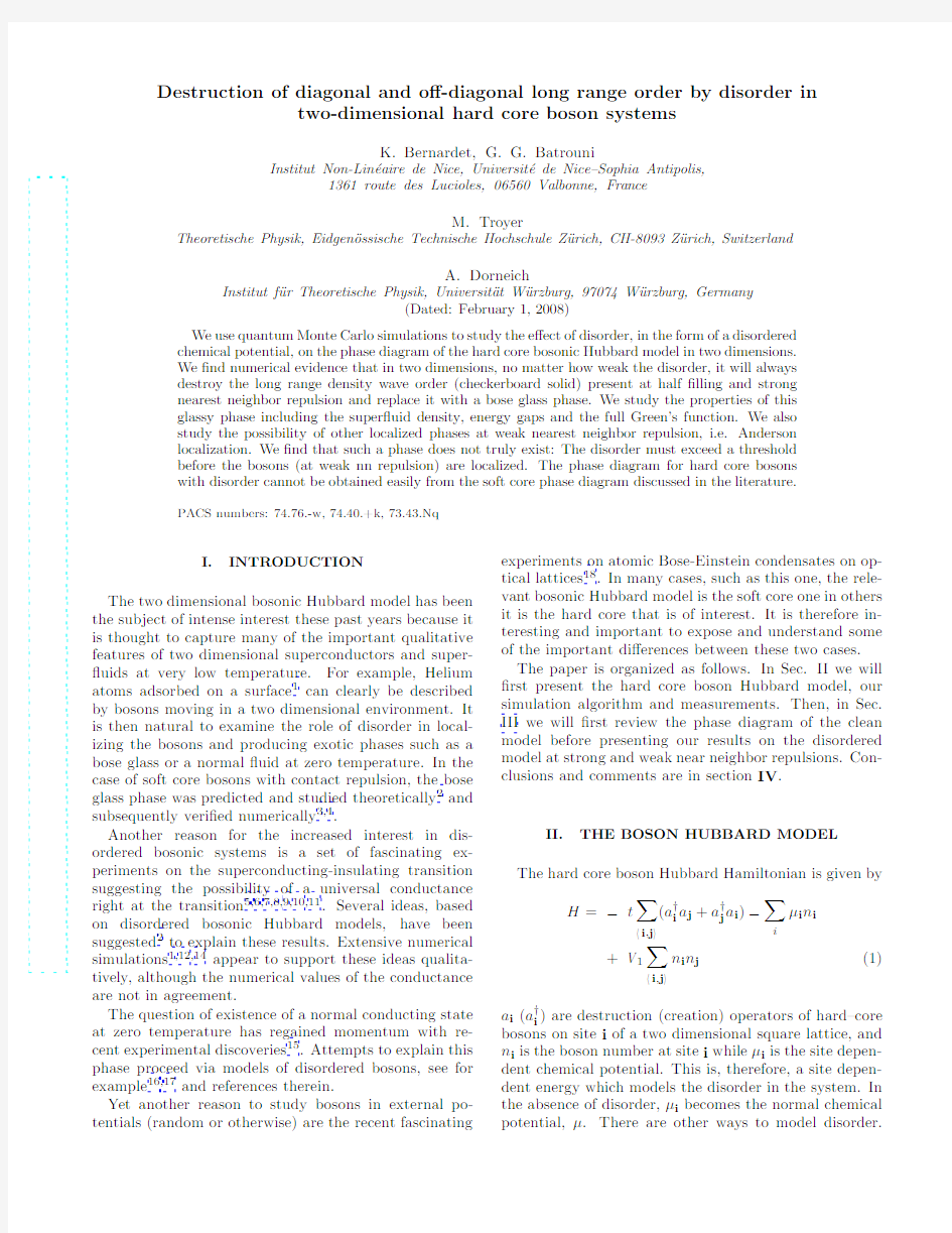
FIG.1:The phase diagram of the hard core bosonic Hubbard model in the absence of disorder(8×8,β=14).Dashed lines indicate?rst order transitions,continuous lines second order transitions.
neighbor(nn)repulsion has been studied extensively in one and two dimensions both with and without disorder. In the absence of disorder,for incommensurate particle ?llings,one always has a super?uid phase.This phase disappears at commensurate?llings(ρ=1,2,3...)when the onsite repulsion is large enough2.The resulting phase is an incompressible Mott insulating phase which takes the form of lobes2,4,21in the(t/V0,μ/V0)plane,where V0 is the onsite repulsion.This phase is gapped,there is a substantial energy cost(increase in the chemical poten-tial)for adding a particle onto a commensurate phase. It was argued2that in the presence of any amount of disorder,a new compressible insulating(i.e.localized) phase,the bose glass,is produced at incommensurate ?llings and that for strong enough disorder the gapped phase disappears entirely.This was subsequently con-?rmed numerically3,4,13,22,23.
The picture changes for hard core bosons with near neighbor repulsion,V.The bosons still form a super-?uid for incommensurate particle?lling and V not too strong.Also,at full?lling,the bosons are always frozen into a Mott insulator since hopping to a neighbor would produce double occupancy which is strictly forbidden. At half?lling,increasing V eventually freezes the bosons into an incompressible gapped checkerboard solid:Alter-nate sites are occupied since the presence of a neighbor costs too much energy and there is a big energy cost(gap) to add a particle.The phase diagram is shown in Fig.1.
A.Strong Near Neighbor Repulsion
We now introduce disorder in the form of a random site dependent chemical potential,μi=μ+δi where the disor-der,δi is uniformly distributed between±?.?is a tun-able parameter characterizing the strength of disorder.
3
the disorder necessary to destroy the checkerboard solid phase and what new phase is produced.One can try to answer this question with a simple argument based on energy balance(Imry-Ma).We start at half?lling with a perfect checkerboard solid and introduce the site dis-order.Suppose that at an empty site there is,due to μi,a deep potential well which pulls in a neighboring boson.This boson will now have near neighbors which it will try push away to rearrange its neighborhood in a local checkerboard solid which will,consequently,have a mismatch at its boundary with the original checker-board.The likelihood of this happening depends on the disorder and dimensionality.The energy cost,in d di-mensions,due to the mismatch at the boundary scales like L d?1for a region of length L.On the other hand, the energy gained by the bosons by falling into locally fa-vorable energy wells scales like L d/2.For d=1,disorder is relevant,no matter how weak it is,it always destroys the solid order.For d=3or more,the energy cost out-weighs the gain and the system maintains checkerboard order.The d=2case is marginal since both,cost and gain,scale like L.Typically,in such marginal cases,the conclusion is that disorder will indeed destroy long range order but just barely.The correlation length,ξ,is very long and the system size should be even larger to see the e?ect.
Numerically,for strong disorder(?/V=2)we can easily see that indeed the gapped checkerboard solid is destroyed on lattices as small as L=12and is replaced by a compressible,glassy insulator with no energy gap. Since for very weak disorder,the system size needed to see the destruction of solid order is too large for us to simulate,we resort to?nite size scaling for the interme-diate disorder case.Although this does not demonstrate directly the validity of the Imry-Ma argument(for which very weak disorder is needed)we believe that the results we will present are qualitatively similar to what happens in the very
weak disorder case.
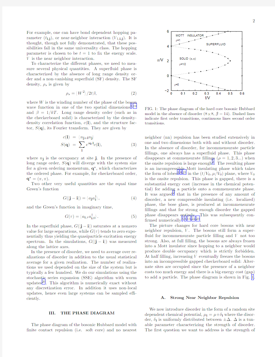
In Figure2we show the density,ρ,as a function of the chemical potential,μ= μi ,for L=8,12,14(β=14) and L=20(β=20)and?/V=1.For L=12,14and 20,we average100disorder realizations,for L=8we did400.We see that the incompressible gapped region (κ=?ρ/?μ=0)gets smaller as L increases but does not quite reach zero.The inset shows the average gap size versus L?1.The average gap size was obtained by cal-culating theρ,μcurve for each realization,which yields the gap size per realization which we then average.An alternative method(which washes out important statis-tical information)is to calculate the averageρ,μcurve and use it to calculate the average gap.We see clearly that the gap tends to zero for a?nite,but large,L.This suggests that,for these values of V and?,the gap will disappear by L≈30.Since L should be greater than ξto observe the destruction of the checkerboard order, we estimate from this thatξ~30.In Figure3we show S(π,π)as a function of L?1.This,again,shows that the
μ
0.4
0.45
0.5
0.55
0.6
0.65
0.7
ρ
FIG.2:ρversusμfor?/V=1and di?erent systems sizes showing the shrinking gap.Inset:The average gap versus L?1.β=14for L=8,12,14andβ=20for L=20
00.040.080.120.16
1/L
0.1
0.2
S
(
π
,
π
)
/
L
2
FIG.3:S(π,π)versus1/L for?/V=1.β=14for L= 8,10,12,14andβ=20for L=20.Long range order seems to disappear for L≥30.
about L=30.
To elaborate this further,we show in Fig.4the distri-butions of the gap sizes for di?erent disorder realizations for L=8,20.We see that for L=8,the distribution is quite narrow and peaked at a nonzero value.How-ever,for L=20,the distribution is very wide and in fact peaked at zero indicating that the most probable value for the gap is zero.In this case,it is incomplete to discuss the“average”of the gap,which is still non-zero.
In order to characterize further the compressible phase which replaces the checkerboard solid,we study the be-havior of the Green’s function,both for equal and un-equal imaginary times.For example,in Figure5we show the equal time Green’s function for V=4.5,L=10and ρ~0.56.We see that the Green’s function goes to zero and is very well?t by an exponential(in fact a hyperbolic cosine to account for the periodic boundary conditions). This is further evidence that there is no super?uid in this
4
05
1015
gap
20
40
60
02468
gap
10
20
30
40(a)
(b)
FIG.4:Gap distribution for di?erent realizations for L =8(β=14,400realizations)(a)and L =20(β=20,100realizations)(b).V =?=4.5.As lattice size increases,the distribution gets very wide and peaked at 0.
r
0.2
0.4
0.6
0.8
(r )a (o )> FIG.5:Equal time Green’s function as a function of distance for L =10,β=20,V =4.5,and ?/V =1.The solid line is a ?t of the form:y =A 0(exp(?(L/2?x )/A 1)+exp((L/2?x )/A 1))with A 0=6.4×10?5and A 1=0.552. The glassy nature of this phase can be seen in the time-dependent Green’s function,Eq.5.In the Bose glass phase,this quantity is predicted 2to decay as G (τ)~1/τ,which has been veri?ed numerically in a very di?erent context 23.Figure 6shows that is also true in this case.Therefore,the new phase replacing the gapped checker-board solid is an ungapped insulating Bose glass phase.Clearly,it is very di?cult to examine these issues with smaller couplings and disorder:The correlation length will be even longer and much larger sizes would be needed.However,for moderate disorder,the above results demonstrate that,whereas it might appear on a ?nite lattice that the gapped solid phase is still present,τ 0.00 0.05 0.10 0.150.20 (0,0)> FIG.6:The Green’s function,G (τ)as a function of imaginary time separation,same parameters as Fig. 5.The solid line is a ?t of the form:G (τ)=A 0(τA 1+(β/2?τ)A 1)+A 2with A 0=0.04,A 1=?1.0and A 2=?0.0065.With a two parameter ?t (excluding A 3)we also get a good ?t with A 0=0.03and A 1=?1.16. large enough systems.We may conclude from this that the Imry-Ma argument holds and that disorder,no mat-ter how weak,will produce a glassy,compressible,un-gapped insulating phase at strong near neighbor cou-plings. B. Weak Near Neighbor Repulsion We now consider the question of what happens when the near neighbor repulsion is decreased and only the hard core and disorder interactions remain.For soft core bosons with no nn interaction,a re-entrant behavior was observed for ρs as a function of the contact repulsion both in one 3and two 4dimensions.In other words,for ?xed disorder strength,as the onsite repulsion is increased from zero,the super?uid density is at ?rst zero,then at some intermediate value of V 0/t the bosons delocal-ize and ρs takes on a ?nite value,then for large enough V 0/t (i.e.approaching the hard core limit)the bosons are localized again.In one dimension this happens for any amount of disorder,but in two dimensions was only reported 4at ?/t =6.This was taken as con?rmation of the phase diagram presented in reference 2where the bosons were argued to be always localized,even by weak disorder,when V 0/t is very large. The phase diagram in the (t/V 0,μ/V 0)plane 2should however be interpreted with care especially if we want to consider the hard core limit.It is a phase diagram at constant ?nite disorder ?/V 0and thus t/V 0→0means that ?/t →∞,and any arbitrarily weak disorder in units of V 0becomes in?nitely strong in the hard core limit.In fact,?gure 7shows that hard core bosons behave dif-ferently,when a ?nite disorder ?/t is considered.While the bosons are localized by weak disorder for large nn 5 r 0.05 0.1 0.15 0.2