? 2000 Psychology Press Ltd
https://www.doczj.com/doc/749082980.html,/journals/pp/13546783.html
Background beliefs and evidence interpretation
Aidan Feeney
University of Durham, UK
Jonathan St.B.T. Evans and John Clibbens
University of Plymouth, UK In this paper we argue that it is often adaptive to use one’s background beliefs
when interpreting information that, from a normative point of view, is incomplete.In both of the experiments reported here participants were presented with an item possessing two features and were asked to judge, in the light of some evidence concerning the features, to which of two categories it was more likely that the item belonged. It was found that when participants received evidence relevant to just one of these hypothesised categories (i.e. evidence that did not form a Bayesian likelihood ratio) they used their background beliefs to interpret this information. In Experiment 2, on the other hand, participants behaved in a broadly Bayesian manner when the evidence they received constituted a completed likelihood ratio.We discuss the circumstances under which participants, when making their judge-ments, consider the alternative hypothesis. We conclude with a discussion of the implications of our results for an understanding of hypothesis testing, belief revision, and categorisation.
INTRODUCTION
Deciding between alternatives is central to our ability to make choices and categorise. It underlies, for example, deciding which university to attend, who to vote for, and whether to get married. In addition, our actions towards people and objects in the world frequently depend on the category to which we decide they belong. A psychiatrist’s subsequent treatment of a client may crucially depend on whether they diagnose the client to be obsessive or depressive. Your decision to go to the beach may depend on what weather the early morning sky seems to promise. Very often, however, we possess incomplete information. For example,
Correspondence should be addressed to Aidan Feeney, Departm ent of Psychology, University of Durham , Science Laboratories, South Road, Durham, DH 1 3LE, UK. Email:aidan.feeney@https://www.doczj.com/doc/749082980.html,
This research was funded by grant R000222426 from the Economic and Social Research Council to the first two authors. We thank Sim on Venn for assistance with the preparation of materials and analysis of results, and Nigel Harvey, Mike Oaksford, and two anonymous referees for their helpful comments on an earlier draft of this paper.
98FEENEY, EVANS, CLIBBENS
we may know that the sky is blue and that many fine days have started with blue skies. We might not know, however, how many days have turned out to be wet given blue early morning skies.
The incompleteness of the information possessed in the beach example is problematic in terms of standard Bayesian approaches to decision making. Bayes’ theorem suggests that we should evaluate the truth of any hypothesised state of affairs against at least one other mutually exclusive and exhaustive alternative possible state of affairs. More than this, it prescribes that we should evaluate any evidence we possess that is relevant to the decision in the light of both alternatives. In other words we need complete information about the implications of our evidence. So, when trying to decide whether or not to go to the beach we need to ask ourselves how likely a blue early morning sky is given (a) that the weather turns out to be good and (b) that the weather turns out to be bad. Specifically, we need to consider the diagnosticity of the information we possess.
Much of the experimental work on hypothesis testing and choosing between alternatives has examined people’s information selection against the background of the normative approach offered by Bayes’ Theorem which we have just informally described. A more formal description is as follows:
P H D P H D P H
P H
P D H
P D H
(/) (/)
()
()
(/)
(/)
=Equation 1
where H and D refer to hypothesis and datum respectively and the ? denotes “not”. From left to right the equation can be read as Posterior Odds equals Prior Odds multiplied by the Likelihood Ratio. The last term—likelihood ratio—is a formal measure of the diagnosticity of the evidence—that is, the extent to which it discriminates between the alternative hypotheses. People’s intuitive under-standing of diagnosticity is considered to be relevant to their capacity to make rational decisions and hence has received attention in the psychological literature on judgement and choice. This literature has been reviewed by Doherty et al. (1996) who point out that the different conclusions about people’s understanding of diagnosticity that have been reached hinge on the extent to which the experi-mental materials used structure the task for participants.
The work which Doherty et al. review is of two types. In the first type participants are asked to select from among pieces of information of differing diagnosticity (e.g. Devine, Hirt, & Gehrke, 1990; Skov & Sherman, 1986; Trope & Bassok, 1982) in order to decide to which of two mutually exclusive and exhaustive categories a target instance belongs. Typically, the most diagnostic information is chosen by participants in experiments of this type. In the second type (Kern & Doherty, 1982; Doherty, Mynatt, Tweney, & Schaivo, 1979; Mynatt, Doherty, & Dragan, 1993), participants are presented with a target
BELIEFS AND EVIDENCE INTERPRETATION99 instance possessing some features and which is said to belong to one of two mutually exclusive and exhaustive categories. They are then given the opportunity to discover the conditional probability of each feature, given each category, i.e. P(D/H) and P(D/?H). The task is structured so that participants may make a limited number of selections from among the available information, and choosing to discover the conditional probability of any feature given one of the categories represents a single information selection.
The question of interest in experiments of this kind is whether participants select pieces of information in pairs. That is, if they select information P(D/H) concerning a certain feature, then, according to investigators such as Doherty, Bayes’ theorem states that they should also select information concerning P(D/?H) for that feature. However, the typical finding with this paradigm is that the majority of people do not select conditional probabilities in pairs. For example, Kern and Doherty (1982) set up a scenario in which medical students had to infer from which of two fictitious diseases (A or B) a patient was suffering. The patient was said to have a high fever and to be covered in a rash. This scenario contains a target instance (the ill patient) and two mutually exclusive and exhaustive alternatives (the disease is either of Type A or of Type B). Next participants were told that 81% of patients suffering from disease Type A display a rash, i.e. P(D1/Ha) = .81—we will refer to the category that this initial piece of evidence concerned as the focal category and to its complement as the non-focal category—and were asked to select just one of the three remaining pieces of information in order to help them decide to which of the categories the target instance belonged. The three remaining pieces of information were as follows:
1.The percentage of patients suffering from disease of Type B who have a
rash P(D1/Hb).
2.The percentage of patients suffering from disease of Type A who have a
high fever P(D2/Ha).
3.The percentage of patients suffering from disease of Type B who have a
high fever P(D2/Hb).
In this simple task participants are given one half of a likelihood ratio [P(D1/Ha)] which they may complete by selecting the first piece of information [P(D1/Hb)]. However, the majority of participants do not select the diagnostic information. Instead they tend to select further information about the focal hypothesis [P(D2/Ha)]. Their findings on experiments of this type have led Doherty and his colleagues to conclude that most people do not possess an understanding of diagnosticity. Furthermore, they have characterised people’s tendency to select incomplete information on the task just described as pseudodiagnostic (for ease of exposition we will refer to the paradigm used by Doherty and colleagues as the PD paradigm). Doherty and colleagues explain
100FEENEY, EVANS, CLIBBENS
pseudodiagnostic selections on the task with reference to a confirmation bias where participants choose information that they consider will provide further support for the hypothesis they are currently considering.
The question that we will address in this paper, is the use to which people put both pseudodiagnostic (incomplete) and diagnostic (complete) information. According to the reading of Bayes’ theorem outlined earlier, in the absence of a completed likelihood ratio, we should not attempt to make inferences about our hypotheses from our data. However, the majority of participants in Doherty’s experiments fail to select probabilistic information in pairs that form likelihood ratios. In addition, several researchers (Beyth-Marom, 1990; Doherty et al., 1996 Experiment 5; Robinson & Hastie, 1985) have shown that people update their beliefs about hypotheses in the light of incomplete information. Accordingly, the first question this paper will address is whether there is a sensible manner in which to interpret pseudodiagnostic information.
The question of whether such a sensible manner in which to interpret pseudo-diagnostic information exists is both important and simple. It is important because although the experiments that have demonstrated pseudodiagnosticity have always been fair to participants by providing them with the opportunity to complete a likelihood ratio, our everyday environment may not always be so kind. Very often we will only have access to one half of a likelihood ratio. If this is the only information available to us then we must decide on the best way to use it.
Intuitively, there is a simple answer to our question concerning how best to interpret pseudodiagnostic information. Most of the time when we are in possession of a single likelihood we are able to interpret that information with reference to our background beliefs. This is in stark contrast to participants in Kern and Doherty’s experiment described earlier. In that experiment materials were chosen to ensure that participants had no such background beliefs to which they could refer.
As an example of how background beliefs may be used to interpret a single likelihood, imagine yourself trying to find a house which you know to be located on either street A or street B and to possess a swimming pool and a garage. If you are told that 95% of houses on street A possess a garage, how confident would you be that the house you are trying to find is on that street? Alternatively how confident would you be if you are told that 95% of houses on street A possess a swimming pool? Intuitively, we suggest, you would be more confident in the latter case than in the former. This is because houses with swimming pools are very rare and the probability that a house on street B will possess one is very low. Houses with garages, on the other hand, are extremely common and it is highly probable that a house on street B will turn out to possess a garage. Thus, your background knowledge about the frequencies of swimming pools and garages
BELIEFS AND EVIDENCE INTERPRETATION101 allows you to be more confident when the information you receive in this example concerns swimming pools than when it concerns garages.
It is informative to contrast our example with the scenario from Kern and Doherty (1982). We contend that it is correct to claim that in the absence of background beliefs Bayes’ theorem specifies that participants must be in possession of a completed likelihood ratio prior to adjusting their beliefs about the hypotheses. However, when in possession of the relevant knowledge about the evidence available, as is likely to be the case in the example, it is broadly Bayesian to use that background knowledge in order to interpret a single likelihood.
In the terms of Bayes’ theorem we are suggesting that, in the absence of a completed likelihood ratio [P(D/Ha)/P(D/Hb)], people will interpret a single likelihood P(D/Ha) with regard to their beliefs about P(D). For the sake of convenience we will refer to people’s beliefs about P(D) as their beliefs about the rarity of the feature that likelihood concerns. In terms of the example, houses with swimming pools are rare while houses with garages are common. Thus, even in the absence of information about the non-focal hypothesis, we know that because swimming pools are rare it is very unlikely that many houses on street B will possess them. Accordingly, we can be confident that the house for which we are looking is on street A. Conversely, as houses with garages are very common it is more likely that most of the houses on street B have garages. Our confidence that the target house is on street B should, therefore, be less in this latter case. We suggest that with incomplete information, rare features are regarded as implicitly diagnostic.
Hence, the first experiment to be reported in this paper will examine whether people’s background beliefs about the rarity of features of objects affects their interpretation of single likelihoods. It will differ, therefore, from the PD paradigm in two ways. First, participants will receive, rather than select, evidence. Second, the materials used will be realistic, in contrast to the mostly abstract materials used by Doherty and his colleagues (e.g. Doherty et al., 1996; Kern & Doherty, 1982; Doherty et al., 1979).
There is some reason to expect that people will be sensitive to the rarity of the features they are reasoning about when interpreting incomplete evidence. Recent research on several variants of Wason’s selection task (Green, Over, & Pyne, 1997; Kirby, 1994; Oaksford, Chater, Grainger, & Larkin, 1997) has shown that the rate at which people tend to turn over the different cards to test the experimental rule is sensitive to the probabilities of the items mentioned in the rule. These findings sit well with theoretical work on hypothesis testing (e.g. Evans & Over, 1996; Klayman & Ha, 1987; Oaksford & Chater, 1994) which suggests that sensitivity to the probabilistic structure of our environment allows us to test hypotheses in an adaptive manner.
102FEENEY, EVANS, CLIBBENS
The categorisation literature also offers support for the claim that people are sensitive to the probabilistic structure of their environment. For example, it has been known for some time that single feature frequencies are encoded in concept learning tasks (e.g. Bourne, 1982; Neumann, 1974). More recently, it has been discovered that single feature frequencies will be encoded even on incidental concept learning tasks (Wattenmaker, 1993).
Recent work on a variant of the PD paradigm (Feeney, Evans, & Clibbens, 1997) gives an even stronger indication that our participants will interpret incomplete information with reference to their background beliefs about the rarity of the features that information concerns. This study differed from the standard paradigm in that deterministic rather than probabilistic evidence was provided. Half of the participants received a scenario such as the following:
Your friend has just bought a new house. You can’t remember whether it’s on street A or street B but you do remember that it has a garden and a swimming pool. The other half were told that their friend’s new house possessed a garden and a garage. Participants in the first half of the experiment were told that houses on street A possessed swimming pools while those in the second half were told that houses on street A possessed garages. All participants were asked to select one further piece of evidence from the remaining three in order to help them decide between the alternatives. The results of this experiment demonstrated that participants given an initial piece of information concerning a common feature (i.e. gardens) were significantly more likely to choose further information con-cerning the focal hypothesis than were participants given an initial piece of information about a rare feature (i.e. swimming pools). In other words, participants in the experiment were less likely to exhibit what Doherty and his colleagues term “pseudodiagnosticity” when they were initially presented with information concerning a rare feature of the object to be categorised. Feeney et al. interpreted their findings by suggesting that participants were choosing information in a broadly rational manner by paying more attention to a rare and therefore implicitly diagnostic feature. Where a feature is common, people may assume that it will be present with the alternative hypothesis and that such information will therefore be of little value. This would lead them to reject the choice considered by Doherty et al. to be diagnostic and normatively correct. However, although the experiment just described suggests that people are sensitive to the rarity of the features when testing hypotheses, it remains an empirical question as to whether they will show similar sensitivity when evaluating the truth of hypotheses. Hence, the first experiment to be reported in this paper will investigate whether people use their background beliefs about the probability of features in the world when interpreting the pieces of evidence that they receive.
BELIEFS AND EVIDENCE INTERPRETATION103
EXPERIMENT 1
Experiment 1 was designed to investigate the intuitions outlined earlier concerning people’s sensitivity to rarity of evidence in a belief revision task. Our participants received two sequential pieces of pseudodiagnostic information—both concerning one of two alternative hypotheses—for two reasons. First, the pseudodiagnosticity effect means that the majority of people, when given the opportunity to do so, do not select pieces of evidence in complementary pairs (Doherty et al., 1979). They tend instead to select those halves of the available likelihood ratios that relate to just one of the available hypotheses. It is thus of interest to examine empirically how people combine and use such pieces of information in order to produce a level of belief in the hypothesis to which they relate.
The second reason for giving participants sequential pieces of pseudo-diagnostic information in this experiment is to enable comparisons between aspects of Experiments 1 and 2. These comparisons will be in terms of any primacy or recency effects present in the results. Order effects in judgement are a very common and widely replicated phenomenon (e.g. Asch, 1946; Lopes, 1985; Stewart, 1965). It is usual in order effect studies for half of the participants to be given strong evidence followed by weak evidence (Strong 1st) and for the other half to be given this same evidence but in the reverse order (Strong 2nd). An order effect is said to have occurred if, after all of the evidence has been received, there is a difference between the two groups in terms of their degree of belief in the hypothesis to which the evidence relates. If Strong 1st participants are more confident that the hypothesis is true then primacy is said to have occurred (e.g. Asch, 1946; Roby, 1967; Tetlock, 1983). If, on the other hand, Strong 2nd participants display more confidence in the hypothesis, then a recency effect has taken place (e.g. Hendrick & Constantini, 1970; Stewart, 1965). The strength of the evidence will be manipulated in Experiment 1 by means of adjusting the likelihood assigned to the evidential features presented. Thus participants will receive information about two features, for one of which the likelihood will always be .95 and for the other .70.
Method
Participants.130 students of the University of Plymouth took part in this experiment. Their mean age was 20 years, they ranged in age from 18 to 44, and 66 of the participants were male, 64 were female.
Design.The experiment had a 2 × 2 × 2 × 3 mixed design. The between-participants manipulations were of the order in which participants received information and the rarity of the features that that information concerned. The order manipulation was achieved by giving participants two pieces of
104FEENEY, EVANS, CLIBBENS
information for each problem. This information was always that 70% of instances of one category possessed one feature and 95% of the same category possessed the other feature. The order in which participants received these pieces of evidence was manipulated. Half of them received the strong information concerning the feature possessed by 95% of instances of the focal category first, while the other half received this information second. For ease of exposition the former level of the order manipulation will be referred to as Strong 1st while the latter level will be referred to as Strong 2nd. The second factor manipulated in this experiment was the rarity of the evidential features used. This was achieved by giving half of the participants information about two rare features of the object to be categorised, while the other half received information about two common features. This manipulation was based on the results of a pre-test (described later) designed to ensure that each feature pair contained features that were perceived to be of approximately equal rarity.
The within-participant variables in this experiment were problem content (all participants completed three problems) and when participants expressed their confidence (time expressed). Each problem contained two rating scales. The first of these scales occurred after receipt of the first piece of evidence, while the second scale occurred after receipt of the second piece of evidence. All participants completed both scales for all problem contents. The levels of the time expressed variable will be referred to as Time 1 and Time 2. There were 33 participants in each between-participants cell of the design, with the exception of the Strong 1st Rare features cell which had 31 participants.
Materials.All participants received a booklet which comprised an instruction sheet and three problems. In each of the three problems, participants were given a scenario involving a decision about which of two alternatives was likely to be the case. Next they received a piece of evidence relevant to the decision and on a rating scale were asked to express their confidence in the alternatives in the light of the evidence they had received. Following this, participants were asked to state their expectations about the remaining unseen evidence. On the next page was a further piece of information relevant to their decision and a second rating scale. Each participant received three problems involving a house, an engineer, and a car. An example of the house materials is:
Your friend has just bought a new house. You can’t remember whether it’s on street X or street Y. You do remember that the house has a garden and a garage. You have the following piece of information: 95% of houses on street X have garages.
Now please look at the scale below which is designed to measure your confidence in each of the decision alternatives in the light of the information you have available to you. One end of the scale corresponds to complete certainty that
BELIEFS AND EVIDENCE INTERPRETATION105 your friend now lives on street X and the other to complete certainty that your friend lives on street Y. Please mark the point on the line that corresponds to your belief about the alternatives. Remember that the greater your confidence in an alternative the closer your mark should be to the end of the scale that corresponds to complete certainty in that alternative.
Next there appeared a rating scale 100 millimetres long labelled at one end “Certain that your friend lives on street X” and “Certain that your friend lives on street Y” at the other. Following completion of the rating scale participants were asked to answer the following questions:
1.What percentage of the houses on street Y would you expect to have a
garage?
2.What percentage of the houses on street X would you expect to have a
garden?
3.What percentage of the houses on street Y would you expect to have a
garden?
The questions concerning participants’ expectations about the unseen evidence were intended as a test of our rarity manipulation. It was predicted that participants’ stated expectations about the percentage of non-focal instances possessing the initial feature (the percentage of houses on street Y that possess a garage in the example) would be higher in the common conditions than in the rare conditions. However, in order that participants would not consider any of the unseen pieces of evidence more important than any other, we asked for their expectations concerning all three remaining pieces. Finally, on the second page of each problem participants were given a second piece of evidence. In this example that information would be:
75% of houses on street X have a garden.
This information was followed by a second rating scale identical to the one on the previous page.
Procedure.All participants completed their booklets in class. Class sizes varied from 10 to 100. In each condition either five or six participants received the problems in each of the six possible orders. They worked on their problems individually.
Pre-test.The pre-test was designed to establish the rarity of certain features of objects for three separate problem contents (concerning an engineer, a house, and a car). A total of 30 undergraduate students (6 of whom were male and 24
106FEENEY, EVANS, CLIBBENS
female) at the University of Plymouth were paid to take part in the pre-test. Their mean age was 27 with the youngest being 19 and the oldest 43. None of these participants took part in any of the experiments reported in this paper. All participants in the pre-test completed their booklets in groups of 5 to 10. These booklets comprised a set of instructions and three sheets, each of which contained a context and a list of features to be rated. The instructions explained the task by means of an example, while at the top of each rating sheet was a question in the following form:
Out of every 10,000 engineers, how many would you expect to…?
This was followed by a list of features for which participants had to give frequency estimates. Each of these lists contained between 8 and 10 features. Mean estimations (in the form of percentages) for the features used in the experimental materials are shown in Table 1.
Results
Manipulation check.In order to check the success of the rarity manipulation the percentage of non-focal items that participants expected to possess the initial evidential feature was analysed using a 2 (Rarity) × 2 (Order) × 3 (Problem Content) mixed factors Anova. The results of this analysis confirmed the results of the pre-test: Expectations concerning the percentage of instances governed by the non-focal hypothesis which would possess the initial feature were significantly lower, F(1, 94) = 4.78, MSE= 950.21, p < .05, when the initial feature was rare (mean = 63. 1, S.D. = 21.0, n = 45) than when it was common
TABLE 1
Perceived rarity of features (Experiment 1)
possess the experim ental features. Column A contains the features used in Experiment 2.
BELIEFS AND EVIDENCE INTERPRETATION107 (mean = 72.0, S.D. = 15.6, n = 53). This result suggests that our rarity manipulation was successful.
Effects of rarity on confidence judgements.For the purposes of the analysis that follows, participants’ judgements expressed on the 100 mm line were converted to scores on a 100-point scale ranging from 1 to 100. Each point on this scale corresponds to one millimetre on the line and the higher a participant’s score on this scale, the more confident she is that the focal hypothesis is the case. Participants’ ratings were analysed using a 2 × 2 × 2 × 3 mixed design Anova. Table 2 contains the mean confidence ratings for the focal hypothesis produced in each cell of the design. There was a significant main effect of rarity on confidence ratings, F(1, 126) = 7.13, MSE= 943.96, p < .01. The mean con-fidence rating for participants who received information concerning two rare features was 68.0 (S.D. = 12.3) whereas the equivalent mean in the Common conditions was 62.1 (S.D. = 12.7). The interaction between Rarity and the Time Expressed variable was not significant, F(1, 126) = .43, MSE = 191.21, p > .5. Hence, the influence of the rarity manipulation was similar both before and after receipt of the second piece of evidence. The Time 1 mean ratings were 65.0 (S.D. = 12.7) for rare information compared with 59.8 (S.D. = 12.4) for common information, while at Time 2 the corresponding ratings were 71.1 (S.D. = 15.5) and 64.6 (S.D. = 15.5). These results strongly support our hypothesis that people are sensitive to their background beliefs about the rarity of the features they are reasoning about when interpreting evidence about those features.
TABLE 2
Confidence ratings (Experiment 1)
in Experiment 1.
108FEENEY, EVANS, CLIBBENS
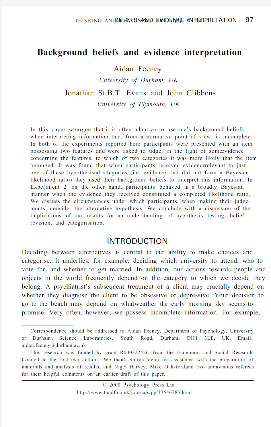
Effects of order on confidence judgements.Unsurprisingly, participants were more confident that the focal hypothesis was the case when in possession of two pieces of information than when they possessed just one. That is, there was a highly significant main effect of Time Expressed, F(1, 126) = 30.56, MSE = 191.21, p < .0001. Mean judgements at Time 1 were 62.4 (S.D. = 12.8) and these increased to 67.8 (S.D. = 15.7) at Time 2. Time Expressed interacted significantly with the Order variable, F(1, 126) = 39.89, MSE= 191.21, p < .0001. This interaction is shown in Figure 1 and clearly indicates a recency effect. Tukey HSDs revealed that participants who received the stronger piece of information second were significantly more confident that the focal hypothesis was the case than were participants who received that stronger piece of information first. In fact, those participants who received the stronger piece of information first showed no increase in confidence in the focal hypothesis upon receipt of the second piece of evidence.
Finally, the Anova produced several significant effects involving problem content. Specifically, a marginally significant interaction between Order and
Figure 1.The interaction between Order and Time Expressed from Experiment 1.
BELIEFS AND EVIDENCE INTERPRETATION109 Problem Content was observed, F(2, 252) = 3.07, MSE = 134.78, p < .05, as well as a significant interaction between Rarity and Problem Content, F(2, 252) = 9.58, MSE = 134.78, p < .0001. Tukey HSDs revealed differences due to Rarity in participants’ ratings for both the house and car materials. No such difference was found for the engineer materials. These results suggest that our pre-test may have been more successful in determining rare and common features for the house and car problems than for the engineer problem.
Discussion
Experiment 1 has provided confirmatory evidence for our predictions concerning the effects of rarity. Specifically, it has shown that people use their background beliefs about the rate at which features of objects occur in the world when interpreting incomplete evidence concerning those features. There is, however, one surprising aspect of our results. The frequency estimates obtained in the pre-test suggest large differences in the perceived rarity of the common and rare features used in this experiment. Although our manipulation check finds these differences to be significant, and there is a significant effect of rarity on confidence ratings, the differences due to rarity observed in the manipulation check and confidence ratings are much smaller than would be expected from the pre-test. This is most likely due to participants’ assumptions about the relation-ship between the hypotheses present in the scenario. Participants may have assumed that the confusion between the hypothesised categories was due to some similarity between them. For example, in the house problem, street A and street B may have been assumed to be close together. As streets in the same neighbour-hood tend to be in the same price bracket and to possess the same amenities, the fact that a large percentage of houses on street A possess a certain feature may have been assumed by participants to increase the probability that a house on street B will also possess that feature. Thus participants’ assumptions about the experimental materials may have attenuated the effect of our rarity manipulation.
Finally, although the highly significant recency effect observed in the confidence ratings of this experiment will be of most interest when comparing the results of this experiment to those of Experiment 2, it does merit some discussion in its own right. Recency under the conditions present in Experiment 1 is predicted by both descriptive (e.g. Anderson, 1981; Shanteau, 1970) and procedural (e.g. Hogarth & Einhorn, 1992; Lopes, 1987) models of belief revision and information integration. In contrast with the influence of back-ground beliefs, which can be argued to be implicitly Bayesian, the recency effect suggests that participants integrated that information in a manner that is at odds with the prescriptions of decision theory. Within this normative framework, the totality of the evidence cannot be affected by the order in which it is received
110FEENEY, EVANS, CLIBBENS
(although see Brown, 1986, and Hilton, 1995, for an explanation of order effects in terms of pragmatic expectations concerning the order in which information is normally presented). In the next experiment we will examine whether people’s judgements are subject to such effects of order when they are based on a completed likelihood ratio.
EXPERIMENT 2
Experiment 2 has three aims. First it seeks to replicate the effects of rarity demonstrated in Experiment 1. Second, Experiment 2 will test whether an already interpreted likelihood will be adaptively reused if the likelihood ratio is subsequently completed. Finally, Experiment 2 will test for the existence of order effects when the individual components of a likelihood ratio are presented sequentially.
To illustrate how we will examine these questions, consider two individuals faced with a judgement task such as that used in Experiment 1: the first judge is told that 95% of houses on street X share a common feature with the house to be categorised, while the second judge is told that 95% of houses on street X share a rare feature with the target house. Based on the results of Experiment 1 we would expect a significant difference between the confidence of these two judges that the target house was on street X. Imagine now that both individuals are subsequently presented with the second half of the likelihood ratio: the first judge is told that 25% of houses on street Y also share the rare feature with the target house, while the second judge is told that 25% of street Y houses also possess the common feature. Both individuals are now in possession of the same likelihood ratio and, according to decision-theoretic prescriptions, regardless of the rarity of the feature for which they possess a likelihood ratio, they should produce identical confidence ratings.
Two simple tests of whether participants adaptively reuse the initial piece of information when interpreting the completed ratio involve looking for effects of order and rarity in participants’ confidence ratings based on the completed likelihood ratio. If use of the completed likelihood ratio is biased by participants’use of their background beliefs to interpret a single likelihood at Time 1 (leading one group of participants to have stronger beliefs in the hypotheses than the other group) then we would expect rarity to significantly affect judgements at Time 2. Similarly, we have already seen that the final confidence ratings in Experiment 1 were subject to a recency effect. If participants are using the completed likelihood ratio in a broadly Bayesian manner, then the order in which they receive the individual components of the ratio should not significantly affect their judgements about the hypotheses.
Finally, we will manipulate the likelihood ratio presented to participants in this experiment. The ratio received will be .95/.60 or .95/.25. This will allow us to
BELIEFS AND EVIDENCE INTERPRETATION111 conduct a separate test on whether order interacts with the value of the completed likelihood ratio in determining participants’ confidence ratings.
Method
Participants.144 students from the University of Plymouth served as participants in this experiment; 68 were male and 75 were female. Their mean age was 23 years. The oldest was 45 and the youngest was 18. All participants were paid for their participation.
Design.The experiment had a 2 × 2 × 2 × 2 × 3 mixed design. The first between-participants manipulation involved the rarity of the feature for which participants were given the likelihood ratio. A target instance possessing both a rare and a common feature was described to participants who were then given information concerning either the common or the rare feature. The second and third manipulations in this experiment involved the likelihood ratio that par-ticipants were given and the order in which that ratio was received. All participants were told that 95% of instances of one category possessed the relevant feature. This being the strongest piece of information that participants received, whether they received it first or second determined whether they were at the Favoured 1st or Favoured 2nd level of the order variable (as this experiment differs from Experiment 1 in that participants receive information concerning both hypotheses, we use the term favoured to refer to the hypothesis that the evidence favours overall). Half the participants were also told that 25% of the non-favoured category possessed the relevant feature, while the other half were told that 60% of instances of the non-favoured category possessed this feature. If participants are sensitive to differences in the likelihood ratio we would predict that once they are in receipt of both pieces of information, those who possess the 95/25 ratio should be more confident that the favoured hypothesis is the case than those given the 95/60 ratio.
As with Experiment 1 the within-participant variables were Time Expressed (Time 1 vs. Time 2 level) and Problem Content.
Materials.Each participant received a booklet comprising an instruction sheet and three problems. The instructions and problem structures used were retained from Experiment 1. The features used are shown in Table 1. As one of the aims of Experiment 2 was to test people’s sensitivity to likelihood ratios for common and rare features, all participants received information about either the rare feature only or the common feature only.
Procedure.The experiment was run with groups of participants ranging in size from 4 to 10 in sessions without a time limit.
112FEENEY, EVANS, CLIBBENS
Results and discussion
Of the 144 participants, one, who received information about a common feature and a likelihood ratio of .95/.60, failed to provide confidence ratings. For the purposes of the analysis that follows, participants’ judgements on the rating scales were treated in the same way as for Experiment 1. Participants’ confidence ratings were analysed using a 2 × 2 × 2 × 2 × 3 mixed design analysis of variance. Table 3 contains the mean confidence ratings from each cell of the design.
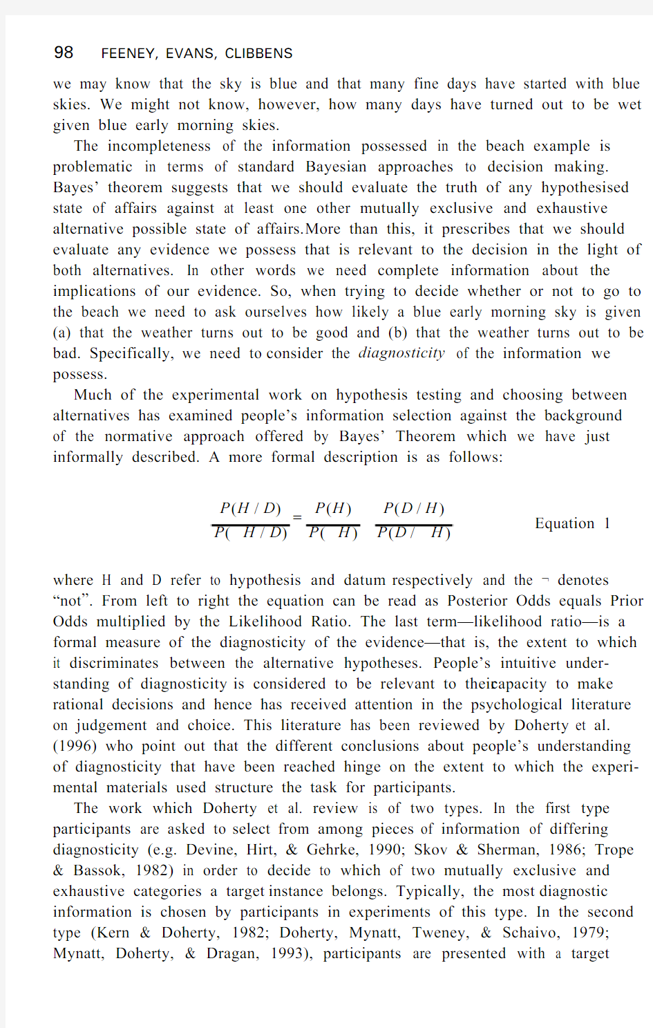
Overall effects of evidence order.There were significant main effects of the Order, F(1, 135) = 16.92, MSE= 484.71, p< .001, and Time Expressed, F(1, 135) = 181, MSE = 364.13, p < .001, variables. Favoured 1st participants produced a mean rating of 67.6 (S.D. = 10.2) whereas Favoured 2nd participants gave a mean rating of 61.5 (S.D. = 8.8). The mean rating at Time 1 was 55.8 (S.D. = 15.4) versus 73.3 (S.D. = 12.4) at Time 2.
More informative is the highly significant interaction (shown in Figure 2) between the Order and Time Expressed variables, F(1, 135) = 74.87, MSE = 364.13, p < .001. Subsequent analyses of simple effects in this interaction
Figure 2.The interaction between Order and Time Expressed from the analysis of subjects’confidence ratings in Experiment 2.
T A
B L E 3
C o n f i d e n c e r a t i n g s (E x p e r i m e n t 2)
113
114FEENEY, EVANS, CLIBBENS
revealed a significant difference between the Order conditions at Time 1, F(1, 135) = 35.43, p < .01, but not at Time 2, F(1, 135) = 1.63.
In contrast to Experiment 1 (see Figure 1) there is no overall recency effect present in the results of this experiment. As the interaction between the Order and Time Expressed factors in Experiment 2 contains a significant difference due to information order only before receipt of the second piece of evidence, it may be inferred that order does not interfere with people’s ability to use the completed likelihood ratio.
Effects of feature rarity.The main effect of rarity, F(1, 135) = 3.98, MSE = 484.71, p < .05 was significant. Participants given information about rare features displayed a mean confidence rating of 66.0 (S.D. = 10.3) whereas par-ticipants given information about the common features gave a mean rating of 63.1 (S.D. = 9.5). As these means are composed of ratings at Times 1 and 2 they are not very informative. More interesting is the significant three-way interaction (displayed in Figure 3) between the Order, Rarity, and Time Expressed variables, F(1, 35) = 4.19, MSE = 364.13, p < .05, which allows us to examine the extent to which rarity affected ratings at Times 1 and 2. Post-hoc Tukey HSD tests for unequal sample sizes revealed that five of the six possible comparisons between ratings produced at Time 1 were significant (the difference between the rare and common levels of the Favoured 2nd participants was not significant). Conversely, only one out of the six possible comparisons between ratings pro-duced at Time 2 proved to be significant (this was the difference between Favoured 2nd participants given the likelihood ratio for a rare feature and Favoured 1st participants given information about a common feature). The pattern of significant differences in this interaction is interesting for several reasons. First, they replicate the results of Experiment 1 where par-ticipants were found to be sensitive to the rarity of the evidential features when interpreting the information they received (as in Experiment 1 the size of the difference due to rarity is not as large as might have been expected from the results of the pre-test). Although the non-significance of the difference due to rarity in the confidence ratings of participants given an initial piece of in-formation concerning the non-favoured category in this experiment is somewhat surprising, it may be due to uncertainty concerning which hypothesis the evidence supports (see Hogarth & Einhorn, 1992; Lopes, 1987). Participants told that 25% of the non-favoured category possessed a rare feature, or that 60% of the non-favoured category possessed a common feature, may have been un-certain as to which hypothesis the information supported.
The second interesting aspect of the interaction between rarity, order and time expressed is the almost complete lack of significant differences between mean confidence ratings expressed after receipt of the second piece of evidence. There does not appear to be a pattern in the results which is directly attributable to the rarity of the features for which participants received likelihood ratios. In stark
BELIEFS AND EVIDENCE INTERPRETATION
115
contrast to the largely systematic differences observed between mean ratings produced before the likelihood ratios were completed, this finding suggests that,once in possession of a full likelihood ratio, participants based their judgements on the ratio itself rather than on the feature for which the ratio was given.Effects of likelihood ratios .The results contained a significant main effect of Likelihood Ratio, F (1, 135) = 12.66, MSE = 484.71, p < .001. Participants given a likelihood ratio of .95/.25 had an overall rating of 67.2 (S.D . = 10.7) versus a rating of 61.9 (S.D . = 8.5) for those participants given a likelihood ratio of .95/.60. Once again, however, as these means comprise ratings produced at Times 1 and 2, this result gives us no indication of participants’ sensitivity to differences in the likelihood ratio.
Of more interest in this regard is the significant three-way interaction (see Figure 4) between the Order, Likelihood Ratio, and Time Expressed variables,
Figure 3. The interaction between Order, Rarity, and Time Expressed from the analysis of subjects’ confidence ratings in Experiment 2.
116FEENEY, EVANS, CLIBBENS
F(1, 135) = 9.59, p < .005. Tukey HSDs for unequal sample sizes revealed that five of the six possible comparisons between confidence ratings expressed prior to receipt of the second piece of evidence were significant. The single non-significant difference was between Favoured 1st participants at different levels of the Likelihood Ratio variable (all participants in these conditions were initially told that 95% of the focal category shared a feature with the target instance). In contrast to the pattern of (mostly) significant differences between means found before receipt of the second piece of information, only two of the six possible comparisons carried out on mean ratings completed after receipt of the second piece of information were significant: Participants in both order
Figure 4.The interaction between Order, Likelihood Ratio, and Time Expressed from the analysis of subjects’ confidence ratings in Experiment 2.