IEEE TRANSACTIONS ON SIGNAL PROCESSING, VOL. 58, NO. 3, MARCH 2010
1171
Singular Value Decompositions and Low Rank Approximations of Tensors
Siep Weiland and Femke van Belzen
Abstract—The singular value decomposition is among the most important tools in numerical analysis for solving a wide scope of approximation problems in signal processing, model reduction, system identi?cation and data compression. Nevertheless, there is no straightforward generalization of the algebraic concepts underlying the classical singular values and singular value decompositions to multilinear functions. Motivated by the problem of lower rank approximations of tensors, this paper develops a notion of singular values for arbitrary multilinear mappings. We provide bounds on the error between a tensor and its optimal lower rank approximation. Conceptual algorithms are proposed to compute singular value decompositions of tensors. Index Terms—Low-rank approximations, multidimensional signal processing, multilinear algebra, tensors.
I. INTRODUCTION ENSORS or multiway arrays are the natural mathematical objects to describe physical quantities that evolve over multiple independent variables. The analysis and approximation of multilinear functionals (tensors) is relevant in many applications, such as data compression, imaging, network analysis, control design and model reduction. This paper proposes techniques to analyze and approximate tensors through the computation of low-rank approximations. For the matrix case (that is, tensors of order 2), the problem of ?nding low-rank approximations is well understood and its solution consists of truncating a dyadic expansion (i.e., a ?nite sum of orthonormal rank one matrices) of the matrix, that is directly inferred from a singular value decomposition of the matrix [11]. For higher-order tensors, this problem has been studied by many authors [7], [10], [15], [16], [21], [25]. With the approximation error de?ned by the Frobenius norm, and with a suitable notion of tensor rank, it was found that the optimal lower rank tensor approximation problem is ill-posed in the sense that optimal low rank approximations may fail to exist or may not be unique. More specifically, it has been shown that the space of rank tensors is non-compact [10] and that the nonexistence of low-rank approximations occurs for many different ranks and orders, regardless of the norm. The existence, uniqueness and computability of optimal low rank approximations of higher order tensors has therefore been recognized as a major problem in numerical multilinear algebra.
T
Manuscript received April 09, 2009; accepted September 05, 2009. First published October 13, 2009; current version published February 10, 2010. This work was supported in part by the Dutch Technologiestichting STW under Project EMR.7851. The associate editor coordinating the review of this manuscript and approving it for publication was Dr. Chong-Meng Samson See. The authors are with the Control Systems group of the Department of Electrical Engineering, Eindhoven University of Technology, P.O. Box 513, 5600 MB Eindhoven, The Netherlands (e-mail: f.v.belzen@tue.nl). Digital Object Identi?er 10.1109/TSP.2009.2034308
Within the existing literature, one can distinguish two main classes of tensor decompositions. The ?rst one is known as a Tucker decomposition [24] and represents an order tensor as the product of a core tensor of the same size as the original one together with nonsingular matrices whose columns span the domain of each of the arguments of . A special case of this decomposition is the higher order singular value decomposition (HOSVD) that has been proposed in [18], [19]. The second class of decompositions amounts to representing as a linear combination of normalized rank-1 tensors (outer-products of norm 1). The latter is usually referred to as a PARAFAC or CANDECOMP decomposition [6], [14]. Both classes of tensor decompositions have been used for lower rank tensor approximation. However, neither of these classes provide optimal low rank approximations as in the matrix case. One can therefore only reach the conclusion that the algebraic and geometric properties of are highly dissimilar. matrices and tensors of order The purpose of this paper is to develop a notion of singular value decompositions for tensors (TSVDs) and to study its implication for the problem of ?nding (optimal) low rank approximations of tensors. We will do this by introducing a decomposition that combines a choice of orthonormal bases in the domain of the tensor with a suitable truncation of its expansion. In addition, we aim to develop suitable computational algorithms for the calculation of such decompositions and prove their stability and convergence properties. The focus on the topic of singular value decompositions for optimal rank approximation problems is most natural for a number of reasons. First, the SVD provides a useful way to numerically implement the algebraic concept of rank of matrices. It is doing this by quantifying near rank de?ciencies or distances to lower rank approximations [13]. Second, singular vectors de?ne orthonormal bases of both the domain and codomain of a linear map in such a way that the matrix representation of this mapping is maximally sparse with respect to these bases. Third, singular values provide relevant information to analyze invertibility and the numerical conditioning of matrices and matrix operations. Fourth, the SVD is well de?ned by performing successive rank-one approximations of a matrix. A widely used generalization of the singular value decomposition to tensors was ?rst introduced in [19] and is referred to as the HOSVD. This decomposition involves the classical singular value decomposition of all possible matrix unfoldings of a tensor. In [19], [20] the authors propose an algorithm to construct the HOSVD and derive lower rank approximations by restricting the domain of the tensor to subspaces spanned by the ?rst few left singular vectors of all possible matrix unfoldings. This procedure is easy to compute and implement, but the resulting low order tensors do not optimally approximate . An upper bound on the approximation error is derived in [19]. Al-
1053-587X/$26.00 ? 2010 IEEE
Authorized licensed use limited to: BEIJING INSTITUTE OF TECHNOLOGY. Downloaded on March 04,2010 at 23:41:08 EST from IEEE Xplore. Restrictions apply.
1172
IEEE TRANSACTIONS ON SIGNAL PROCESSING, VOL. 58, NO. 3, MARCH 2010
though the basic idea behind tensor unfoldings is interesting, at a more fundamental level it involves replacing the multilinear structure of a tensor by multiple bilinear structures and, therefore, hides the intrinsic multilinear and algebraic properties of a tensor. More recently, Chen and Saad advocate in [7] a notion of tensor SVD that requires the core tensor to be a diagonal tensor of the same size as the original one. In [7], the authors derive low rank approximations from a decomposed tensor assuming that a diagonal core tensor exists. Unfortunately, diagonalizing transformations do not exist in general and diagonal core tensors only occur in a limited number of applications. Especially in the signal processing community, tensors are commonly viewed as multilinear arrays and tensor operations are carried out with regular matrix manipulations. Although useful for many applications in signal processing [9], [25], [26], this point of view has serious shortcomings when studying tensors at a more fundamental algebraic level. Since changes of coordinate systems are among the most elementary algebraic operations, we believe that it is particularly important to understand tensors as general multilinear functionals in a coordinate-free algebraic context. Therefore, a discussion on coordinate-free concepts such as inner products, orthogonality, contractions, modal ranks and norms of tensors precedes the de?nition of a singular value decomposition and aims to provide insight in the true and more subtle nature of tensors as operators. This paper contributes on explicit upper and lower bounds on the approximation error between a tensor and its lower order modal rank approximations (see below). Optimal approximation results are inferred for rank-1 approximations of tensors and we discuss a method of successive rank-1 approximations. A computational scheme and an explicit power-type algorithm for the computation of singular value decompositions of general tensors is proposed and its convergence properties are discussed. The merits of the algorithms and approximation results are demonstrated on an example of MRI data compression. This paper is structured as follows. Properties, notation and various algebraic concepts related to tensors and their decompositions are collected in Section II. Optimal low rank approximation problems for tensors are formulated in Section III. Section IV introduces the concept of singular values for tensors together with a number of basic properties and characterizations. Main results on tensor approximations are given in Section V. Algorithms and computational issues are discussed in Section VI. An application to data compression of a three-dimensional MRI scan is discussed in Section VII. Finally, conclusions and recommendations are summarized in Section VIII. II. TENSORS AND TENSOR DECOMPOSITIONS A. Tensors An ordertensor is a multilinear functional
where, for each ranges from 1 till . The elements of are commonly encoded in the -way array which, in the signal processing community, is often taken as a (coordinate-dependent) de?nition of the tensor. The represent with respect to a speci?c collecelements tion of bases (1) , respectively, in the sense that . Throughout, the set of all order- tensors on is denoted by which naturally becomes a vector space over when equipped with the standard de?nitions of addition and scalar multiplication. of B. Tensor Norms To formulate optimal approximation problems for tensors, a . For this, suppose that norm is introduced on the space is equipped with an inner product and let denote the corresponding induced norm. We assume this structure to . The operator norm of be available for is de?ned by
That is, re?ects the maximal amplitude that a tensor can assume when ranging over the Cartesian product of all unit . This norm satis?es the properspheres in ties only if for any scalar and for any . Therefore, becomes a normed linear space. The inner product of two tensors with elements and , both de?ned with respect to the bases (1), is given by
It is immediate that the right-hand side of this expression is invariant under unitary basis transformations (i.e., transformations for which for all ) and so becomes a well de?ned inner product space. In fact, after bases for have been decided upon, the above inner product reduces to the inner product of -way arrays as de?ned in, e.g., [19], [20]. Following standard terminology, the induced norm
is called the Frobenius norm (or Hilbert-Schmidt or Schur norm). One infers that
de?ned on vector spaces over . That is, is a linear functional in each of its arguments. In the ?nite dimensional case where is referred to as an (covariant) tensor with the -mode dimension of . Elements of are speci?ed by real numbers
if and only if every basis in the collection (1) is orthonormal. This shows that the Frobenius norm coincides with the ‘higherorder tensor norm’ de?ned in [19], provided that the tensor is represented with respect to orthonormal bases.
Authorized licensed use limited to: BEIJING INSTITUTE OF TECHNOLOGY. Downloaded on March 04,2010 at 23:41:08 EST from IEEE Xplore. Restrictions apply.
WEILAND AND VAN BELZEN: SINGULAR VALUE DECOMPOSITIONS AND LOW RANK APPROXIMATIONS OF TENSORS
1173
It is important to note that both the operator norm and the Frobenius norm are invariant under unitary basis transformations. C. Orthogonality and Tensor Decompositions Consider, for ?xed elements functional , the
. . The elements of . Consequently
Let then satisfy
Then is a tensor in that will be denoted by and is usually called the outer product of . Whenever nonzero, such a tensor will be referred to as a rank-1 tensor. With respect to the bases (1), the elements of are and its norm . Rank-1 tensors will be used as elementary objects to decompose general tensors. For this, we distinguish between different types of orthogonality (e.g., [15] and [17]). and De?nition II.1: Let be two rank-1 tensors. 1) and are said to be orthogonal, denoted , if . 2) They are said to be completely orthogonal, denoted , if for all . The different notions of orthogonality lead to different tensor is said to be decompositions. Speci?cally, a tensor decomposable if there exists an integer and a collection of nonzero constants, , such that (2) If, in addition, and (or ) for then is said to be orthogonal decomposable (respectively, completely orthogonal decomposable) and we refer to (2) as an orthogonal decomposition (respectively, completely orthogonal decomposition) of . Every is decomposable, but orthogonal or completely orthogonal decompositions do not necessarily exist. See [15] for more details. The Frobenius norm is characterized by
which is the tensor evaluation. D. Tensor Contractions and Transformations Let and consider, for mappings where inner product space of dimension posite tensor, denoted de?ned by , the linear is a ?nite dimensional . The com, is the mapping
The composite tensor is an orderthat admits the representation
tensor on
with respect to the bases of the vector spaces . Here, is the th entry in the matrix representation of with respect to the given bases for and . Hence, the multiway array coincides with the usual -mode multiplications of an -way array with matrices as they occur in the signal processing literaand whenture. It is immediate that ever is contractive for all , i.e., for all . E. Tensor Rank The concept of tensor rank is a highly nontrivial extension of the same concept for linear mappings and has been discussed in considerable detail in, for example, [10], [15], [16], [19], [20], [21]. The rank of , denoted , is the minimum integer such that can be decomposed as in (2). By de?nition, the rank of the zero tensor is 0. [15] also introduces the concepts of orthogonal and complete orthogonal rank. The orthogonal rank and complete orthogonal rank of a tensor is the minimal integer in an orthogonal, or completely orthogonal decomposition (2) of (whenever they exist). To de?ne the modal rank of a tensor , we ?rst introduce the -mode kernel of to be the set
and it is easy to see that for any orthogonal or completely orthogonal decomposition (2) of . The following lemma proves useful and relates tensor evaluations with tensorial inner products. Lemma II.2: Let and for . Then
Proof: With respect to the standard bases (1) the tensor evaluation can be written as
Authorized licensed use limited to: BEIJING INSTITUTE OF TECHNOLOGY. Downloaded on March 04,2010 at 23:41:08 EST from IEEE Xplore. Restrictions apply.
1174
IEEE TRANSACTIONS ON SIGNAL PROCESSING, VOL. 58, NO. 3, MARCH 2010
The multilinearity of implies that is a linear subspace of . The -mode rank of , is de?ned by
and is a coordinate free generalization of the -rank in [19]. Note that coincides with the dimension of the space spanned by stringing out all elements till (where the indices are at the th spot). Finally, the modal rank of , denoted , is the vector of all -mode ranks, i.e., . The rank and modal rank are well de?ned in that there exist and for any unique numbers . Obviously, for a rank-1 tensor . For we have that and there exist examples with strict inequality for all [18], [19]. For order-2 tensors (matrices) we have that and the rank concept coincides with the usual notion of rank (row-rank or column-rank) of a matrix. of modal rank For the expression (3) is called a modal rank decomposition of whenever
of rank such that is minimal. These problems are trivial for and completely understood for . Indeed, for the latter case, any admits a representation for some matrix of rank . If
is a singular value decomposition of , then for any pair and any real number the truncated expansion with de?nes the order-2 tensor that solves P1 and P3 provided that and solves P2 and P4 provided that . The corresponding errors are given by and , respectively. For , Problem P4 has been studied in [15], [16], [21], [10] by introducing orthogonal rank-1 tensor decompositions. It was found that the minimum rank approximation problem is ill-posed in that optimal lower rank approximations do not need to exist. In [21] an example is given of a rank 6 tensor for which , showing that the space of lower rank tensors is not closed. For further discussions on Problem P4 we refer to [10], [7]. In this paper we focus on the problems P1 and P2. IV. A SINGULAR VALUE DECOMPOSITION FOR TENSORS A. De?nitions
for . A modal rank decomposition is therefore a representation of with respect to orthonormal bases . The modal rank decomposition is a higher-order extension of the Tucker decomposition introduced in [24] with additional orthogonality constraints. Among the different notions of tensor rank that we de?ne here, only the modal rank can actually be computed for arbitrary order- tensors. The other rank concepts can only be determined for small academic examples such as 2 2 2-tensors. III. PROBLEM FORMULATION The problem of ?nding lower modal rank approximations of a given tensor is the prime motivation for the present work. A precise formulation is given as follows. Problem III.1: Let be a given -order tensor. P1: Given a vector of integers , determine and ?nd, if possible, a tensor with such that is minimal. P2: Given a vector of integers , determine and ?nd, if possible, a tensor with such that is minimal. P3: Given an integer , determine and ?nd, if possible, a tensor of rank such that is minimal. P4: Given an integer , determine and ?nd, if possible, a tensor
be an order- tensor de?ned on the ?nite diLet where we suppose that mensional vector spaces . The singular values of , denoted , and are de?ned as with follows. let For
denote the unit sphere in by
. De?ne the ?rst singular value of (4)
is continuous and the Cartesian product of unit spheres is a compact set, an extremal solution of (4) exists (i.e., the supremum in (4) is a maximum) and is attained by an -tuple
Since
Subsequent singular values of manner by setting
are de?ned in an inductive
Authorized licensed use limited to: BEIJING INSTITUTE OF TECHNOLOGY. Downloaded on March 04,2010 at 23:41:08 EST from IEEE Xplore. Restrictions apply.
WEILAND AND VAN BELZEN: SINGULAR VALUE DECOMPOSITIONS AND LOW RANK APPROXIMATIONS OF TENSORS
1175
for
, and by de?ning
an order-1 tensor (a linear functional) that maps satis?es (5)
to
and
Again, since the Cartesian product
where the “dot” is at the th spot. By the multilinearity of the is independent of . Hence, tensor, rewriting (8) for each independent modal direction gives that satis?es, for
is compact, the supremum in (5) is a maximum that is attained by an -tuple (9a) (9b) It follows that the vectors are mutually or. If for any , then we extend the thonormal in to a complete collection of orthogonal elements . This construction thus leads to a orthonormal basis of collection of orthonormal bases , It follows that i.e., all Lagrange multipliers coincide. Moreover, (9a) implies that for each
(6) for the vector spaces , respectively. De?nition IV.1: The singular values of an ordertensor are the numbers with de?ned by (4) and (5). The singular vectors of order are the extremal solutions in that attain the maximum in (5). A singular value decomposition (SVD) of the tensor is a representation of with respect to the basis (6), i.e., (7) The -way array singular value core of in (7) is called the .
whenever
In a similar manner, for we associate with the optimizadetion problem (5) the Lagrangian ?ned by
where given by
and
is
B. Characterization of Singular Vectors by Duality This section aims to characterize the singular values and singular vectors of tensors of any order. Let and associate with the optimization problem (4) the Lagrangian by setting Again, there exist -tuples stationarity condition . . .
and
that satisfy the (10)
It has already been argued that an -tuple exists that attains the maximum in (4). From the theory of variational analysis [4], [12], one then of infers the existence of an -tuple Lagrange multipliers such that (8) where derivative denotes the gradient of . The -mode Fréchet of at the point is
Rewriting (10) for each modal direction gives for
(11a) (11b) (11c)
Authorized licensed use limited to: BEIJING INSTITUTE OF TECHNOLOGY. Downloaded on March 04,2010 at 23:41:08 EST from IEEE Xplore. Restrictions apply.
1176
IEEE TRANSACTIONS ON SIGNAL PROCESSING, VOL. 58, NO. 3, MARCH 2010
This immediately implies that and we conclude again that, for ?xed , the Lagrange multipliers coincide and are equal to the th singular value. Moreover, for
(12)
where
is the th entry in the vector
.
C. Properties and Examples The following theorem summarizes a number of properties of the tensor singular value decomposition. Theorem IV.2: admits a singular value decom1) Every tensor position. The singular value decomposition (7) is an orthogonal decomposition where the singular values are or. Here, dered according to and the singular vectors of any order satisfy (9) and (11). 2) . 3) For all there holds
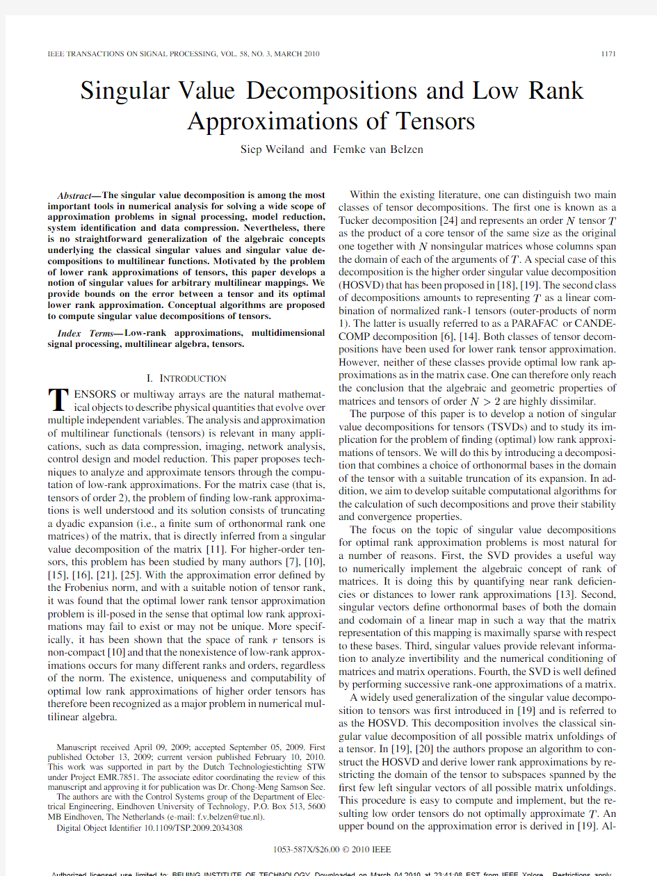
Fig. 1. Visualization of the zero elements in the singular value core of an arbitrary order-3 tensor of dimensions (3, 3, 3).
whenever 4) The singular value core of
. satis?es
5) If in the singular value core of
then the number of zeros is at least
Proof: The existence of the basis has been proven in the previous subsection. The ordering of the singular values and the fact that all rank-1 terms in the decomposition (7) are orthogonal is immediate from the de?nition (5). Item 2 follows from (9) and (11) and the observation that for ?xed , the Lagrange multipliers coincide with (see Subsection IV-B). Item 3 has been derived in (12). Since , it follows that whenever . This is the ?rst case in item 4. To prove the inequality in item 4, let and suppose, without loss of generality, that . Then, for all ,
Substitute for the singular vector . Since we have that , i.e., . It thus follows that as claimed. If then there exists for which . For this we have and consequently, . The fourth case in item 4 follows again from (12). Indeed, if then and, using orthonormality of the bases, and hence by (12). Item 5 follows from (12). Indeed, if then (12) shows that the singular value core tensor vanishes at entries in its th mode. The total number of zero entries of an order tensor is therefore as claimed. In words, any tensor admits an SVD with at most nonzero singular values. In any singular value decomposition of , the ordered singular values occur on the main diagonal of the -way array of elements of the tensor. In general, the singular value core tensor has nonzero entries on its non-diagonal elements. Absolute values of non-diagonal entries are bounded from above by the singular value of index equal to the smallest integer in the core index. Only if (the matrix case) the singular value core tensor is diagonal. A visualization of the zero-structure in an order-3 singular value core is given in Fig. 1. Example IV.3: Any admits a representation where . An SVD of is then given by a representation of with respect to the orthonormal bases and that consist of the ordered columns of the orthogonal matrices and that de?ne a (any) singular value decomposition of the matrix . In particular, by item 4 of Theorem IV.2, the singular value core of coincides with as it has the nonzero singular values of on its main diagonal and is zero for all other elements. For a tensor SVD therefore coincides with the matrix SVD. Example IV.4: Let the tensor with vector spaces have coef?cients and
Authorized licensed use limited to: BEIJING INSTITUTE OF TECHNOLOGY. Downloaded on March 04,2010 at 23:41:08 EST from IEEE Xplore. Restrictions apply.
WEILAND AND VAN BELZEN: SINGULAR VALUE DECOMPOSITIONS AND LOW RANK APPROXIMATIONS OF TENSORS
1177
with respect to the standard Euclidean bases on . A computation of the singular vectors associated with yields the orthonormal bases
In particular, is an optimal solution to problems P2 and P4. where is the Moreover, the error ?rst singular value of . Proof: Let be an arbitrary rank-1 tensor. Then can be written as where and is a normalized rank-1 tensor in that . Using the de?nition of the Frobenius norm, we have
of and , respectively, where . A representation of with respect to this basis gives the singular with singular values and value decomposition of and singular value core
This is a convex function in . But then
that attains its minimum at
Note that the singular values are on the ‘main diagonal’ entries of the core, and that not all off-diagonal entries are zero. Example IV.5: Consider a 2 2 2 tensor that is represented with respect to the standard bases in with the elements and with all other elements zero. Then has singular values and and it turns out that the standard basis de?nes a singular value decomposition of . That is, is already in SVD form and is the singular value core tensor of . Observe that , the singular value core is not diagonal and zero entries. it has V. LOW RANK APPROXIMATIONS This section establishes a number of lower rank approximation results for an arbitrary tensor . Throughout, it is assumed that is a given tensor in of modal rank . Further, (6) is a collection of bases of singular vectors of and we de?ne the subspaces
where the last equality follows from Lemma II.2. The latter expression shows that minimizing over all rank-1 tensors with is equivalent to maximizing over all unit vectors . But this problem is (4) and has as its optimal solution. Consequently, and it follows that is the optimal rank-1 approximation of . The error . Theorem V.2 is particularly useful to de?ne an algorithm of . successive rank-1 approximations of a given tensor Indeed, for given , let denote the optimal rank-1 tensor as de?ned in Theorem V.2. The error then belongs to and is minimal in Frobenius norm when with ranging over all tensors of the form of rank-1. For successive values of , apply Theorem V.2 to the error tensor to de?ne as the optimal rank-1 tensor that minimizes the criterion over all rank-1 tensors . Then set . De?nition V.3: Given , the th order successive rank-1 approximation of is the tensor (14)
De?nition V.1: For a vector of integers with , the modal truncation is de?ned by the restriction and is represented by the expansion (13) where is the singular value core tensor of .
where
are optimal rank-1 approximations of , respectively, as de?ned in the previous para-
A. Successive Rank-1 Approximations The following theorem establishes that modal truncations of rank 1 are optimal solutions to problems P2 and P4. Theorem V.2: Let and . Then the modal truncation is a rank-1 tensor in that is optimal in the sense that
graph. In this construction, the Frobenius norm of the error satis?es the recursion with . In particular, so that the norm of successive approximation errors is non-increasing. Remark V.4: The rank-1 modal truncation de?ned in Theorem V.2 is not optimal in the induced norm. That is, the rank-1 modal truncation does not solve problems P1 and P3 for . B. One Modal-Rank Approximations The following result establishes a lower bound on the approximation error between a tensor and its modal truncation when only one modal rank is reduced.
Authorized licensed use limited to: BEIJING INSTITUTE OF TECHNOLOGY. Downloaded on March 04,2010 at 23:41:08 EST from IEEE Xplore. Restrictions apply.
1178
IEEE TRANSACTIONS ON SIGNAL PROCESSING, VOL. 58, NO. 3, MARCH 2010
Theorem V.5: Let and let
have modal rank
with
. Then
Proof: Without loss of generality assume . De?ne . Then
and
where we used the de?nition of , Lemma 12, and the fact that, satis?es . Furthermore, since it follows that
not every is diagonalizable. If 2) For is diagonalizable, then the singular value core tensor of is, in general, not diagonal. 3) If is diagonalizable with respect to a collection of orthogonal bases, then the singular value core tensor of will be diagonal. Proof: 1) Every can be written as for some matrix . Let be an SVD of . Then the singular value core tensor of is given by the diagonal matrix . 2) A counterexample is given in Example V.8 below. is an orthogonal full rank matrix, 3) Suppose that such that becomes diagonal. Then and is unitary for any permutation matrix of dimension . Now, remains diagonal and the permutation matrices can be chosen such that the diagonal elements of are non-increasing. is then the singular value core tensor of and the columns of de?ne the -mode singular vectors. Example V.8: An example of the second item of Theorem V.7 is given by the tensor de?ned in Example IV.5. As already shown, the singular value core of is not diagonal. However, with respect to the bases
Consequently, . This yields the result. Remark V.6: One consequence of De?nition IV.1 is that the computation of the singular vector of order not only depends on singular vectors of order but also on the singular vectors for and . If modal truncations in one speci?c modal direction, say the th, are searched for, then the coupling of the constraints in the computation of the singular vectors of order may actually prevent the modal truncation de?ned in Theorem V.5 to be optimal. A weakening of the constraints on the set in (5) may then become an alternative. A modi?ed singular value decomposition can be for obtained by rede?ning the set by, for example,
one easily shows that admits a diagonal representation with diagonal elements and . Hence, a diagonalizable tensor will not necessarily have a diagonal singular value decomposition. is diagonalizable with respect to an Theorem V.9: If orthonormal basis, then 1) the rank and orthogonal rank of are equal. 2) the singular value decomposition of is a completely orthogonal rank decomposition. 3) the singular value decomposition of is given by
where is equal to the rank of . The modal truncation de?ned in (13) is represented as
and by performing the optimization in (5). C. Approximation of Diagonalizable Tensors represented with The diagonal of an arbitrary tensor respect to the bases (1) is given by the elements with . We will say that a tensor is diagonal if only its diagonal elements are nonzero. Whenever a collection of bases can be found such that is diagonal we will say that is diagonalizable. When considering higher-order statistics in the problem of Independent Component Analysis, diagonal tensors are of considerable importance. See, e.g., [8], [18], [7]. Theorem V.7: Let , then 1) Every is diagonalizable. Moreover, the singular value decomposition of gives a singular value core tensor that is diagonal. and is an optimal rank- approximation of that in the sense
Moreover,
That is, the modal truncation problems P1, P2, P3, and P4.
is an optimal solution to
Authorized licensed use limited to: BEIJING INSTITUTE OF TECHNOLOGY. Downloaded on March 04,2010 at 23:41:08 EST from IEEE Xplore. Restrictions apply.
WEILAND AND VAN BELZEN: SINGULAR VALUE DECOMPOSITIONS AND LOW RANK APPROXIMATIONS OF TENSORS
1179
Proof: Item 1 is proven in [15]. For item 2 see [27]. To see be an orthonormal basis item 3, let for which has a diagonal representation where the diagonal are assumed to be ordered in that entries . The error tensor is then given by . This gives and which are minimal in view of the ordering of the singular values. See also [27]. VI. ALGORITHMS AND COMPUTATIONAL ISSUES In this section we propose an ef?cient algorithm for the computation of a singular value decomposition of an arbitrary . The algorithm is based on the ?xed order- tensor point properties of a contractive mapping that is iterated in a power-type algorithm to compute the singular vectors of order and the singular values as de?ned in De?nition IV.1. and , we denote by the vector With in . To simplify notation, let and de?ne the mapping by
Then
for , which shows that is ?xed point of . The result of Theorem VI.1 gives rise to the following TSVD algorithm for the computation of a singular value decomposition. INPUT Tensor with -mode dimension . DESIRED A singular value decomposition of . , order Step 0 (Initialization) Set tolerance level , and . Step 1 Select random elements and with and . Set . , and iterate Step 2 Let be de?ned by (15) with the map (17) where is such that Step 3 Write . and de?ne, for
. . .
(15)
Here, is the -mode gradient of in the point (i.e., the transpose of the -mode Fréchet derivative of ). Then is well de?ned provided that for any and . The following theorem relates the ?xed points of to solutions of equations in the Lagrangian system (9). the is a ?xed point of if and only if Theorem VI.1: satis?es the Lagrangian conditions (9) with . is Proof: Only if: Suppose from which it fol?xed point of . Then and lows that for all . . Since the 1-mode Fréchet Consider these equalities for it follows derivative that
Step 4 De?ne the tensor
and set to . Step 5 Repeat Step 1, Step 2, Step 3, Step 4 until . Step 6 For every for which complement to an orthonormal matrix . Step 7 De?ne
(16) we infer that so that we conclude . In a similar fashion one shows that that for all . This gives (9b). But with unit norms, which is (9a) with (16) reads . The same argument applies to prove (9a) for other . vectors If: Suppose a set of satis?es and By taking
Theorem VI.2: Suppose that maps a into itself and that is contractive on closed subset in the sense that there exists such that for all . Then the iteration (17) converges of in . In that case, for each to a unique ?xed point the vectors with satisfy the Lagrangian conditions (11). The statements on the convergence of the iteration (17) can be found in [23]. Theorem VI.2 states that whenever (15) is a contractive mapping on a suf?ciently large closed invariant set then the iteration (17) converges to the solution of the Lagrangian systems (9) and (11). It is easy to see that contractivity
Authorized licensed use limited to: BEIJING INSTITUTE OF TECHNOLOGY. Downloaded on March 04,2010 at 23:41:08 EST from IEEE Xplore. Restrictions apply.
1180
IEEE TRANSACTIONS ON SIGNAL PROCESSING, VOL. 58, NO. 3, MARCH 2010
TABLE I RELATIVE APPROXIMATION ERROR, (k
W 0 W k )=(kW k
)
Fig. 2. 10th slice of the original data.
TABLE II NUMBER OF ITERATIONS
i
OF
(17)
of (15) with implies contractivity of (15) for with . In practice it is not trivial to explicitly verify this condition and to ?nd a closed invariant region that makes contractive. However, Theorem VI.2 promises that whenever the algorithm converges, it converges to a solution of the Lagrangian systems (9) and (11). The algorithm is easy to implement and has shown satisfactory performance. A comparison to an algorithm for the computation of high-order singular value decompositions in [19] will be subject of a different paper. Remark VI.3: We remark that singular vectors and singular values of necessarily satisfy the Lagrangian systems (9) and is positive de?nite, these conditions (11). If the Hessian are also suf?cient in which case one can conclude that the vecwith are indeed the desired singular vectors is the corresponding singular value. tors of order and that Remark VI.4: An algorithm for the computation of succesof as de?ned in sive rank one approximations De?nition V.3 is immediate from Algorithm TSVD. Indeed, for the computation of a rank-1 optimal approximant, only steps 1, 2, and 3 of the TSVD algorithm are relevant. First apply the to result in the optimal approxiTSVD algorithm on mation . Then repeat the TSVD algorithm on the error tensor for to de?ne (14).
in this paper and the method of Successive Rank-one approximations discussed in Section V-A. We aim for a drastic compression of the data. All simulations discussed in this section have been carried out with an accuracy setting of in the TSVD algorithm. Implementations of all algorithms use the tensor toolbox for Matlab [3]. A. Approximations of the Form Table I shows the relative approximation errors in Frobenius norm that were obtained with HOSVD, Successive Rank-One and Tensor SVD respectively. From this it is obvious that HOSVD and Successive Rank-One give comparable approximation errors and outperform the Tensor SVD. The data compression in these approximations is substantial. Indeed, implies a the modal rank approximation with core tensor of 1000 elements, which is 0.05% of the number and therefore amounts to a storage reduction of entries in from 2 MB to 1 KB. Table II lists the number of iterations required in step 2 of the TSVD algorithm for the computation of the Tensor SVD and the various Successive Rank-one approximations. Due to space limitations only the number of iterations for the ?rst ?ve steps of the respective algorithms are shown. The number of iterations seems to be increasing as the algorithm progresses, but this is pure coincidence. The number of iterations decreases and increases quite randomly. The time to compute the ?rst ?ve singular values and sets of singular vectors for this example was 74.05 s on a 1.83 GHz Intel Duo Processor T2400. The ?rst ?ve successive rank-one approximations have been computed in 46.21 seconds on the same PC. B. Approximations of the Form In applications it may be desirable to leave the mode rank unchanged for one or more modal directions. For example, when considering spatial-temporal data, one may be interested in approximating spatial information only. To this end, this section
VII. SIMULATION EXAMPLE To illustrate the methods discussed in this paper, we consider a data compression problem in 3-D imaging1. The data consists of pixel intensities of an MRI scan of a human head in which slices is an image of pixels. The original each of the and , MRI scan has dimensions consists of 1990676 pixels which corresponds to 2 MB of storage. All pixel intensities are stored in an tensor of modal rank . The 10th slice of the original data is shown in Fig. 2. We consider two kinds of approximations to this data. First, we discuss by tensors of modal rank . approximations of Second, we review approximations by tensors of modal rank , i.e., only the ?rst and second mode dimensions are approximated. For both types of approximations we compare the HOSVD [19], the Tensor SVD as introduced
1The data was obtained from TU/e-BME, Biomedical Image Analysis, in collaboration with Prof. Dr. med. Berthold Wein, Aachen, Germany
Authorized licensed use limited to: BEIJING INSTITUTE OF TECHNOLOGY. Downloaded on March 04,2010 at 23:41:08 EST from IEEE Xplore. Restrictions apply.
WEILAND AND VAN BELZEN: SINGULAR VALUE DECOMPOSITIONS AND LOW RANK APPROXIMATIONS OF TENSORS
1181
TABLE III RELATIVE APPROXIMATION ERROR, (k 0 APPROXIMATIONS OF THE FORM (
W W k )=(kW k r ;r ;L )
), FOR
Fig. 3. 10th slice of rank-(10, 10, 29) approximant, computed using HOSVD (left) and Successive Rank-One approximations (right).
Fig. 4. 10th slice of rank-(10, 10, 29) approximant, computed using TSVD (left) and modi?ed TSVD (right).
gives simulation results for approximations of the form for the MRI data. As in the previous section, a comparison is made between the HOSVD, Tensor SVD and the method of successive rank-one approximations. Furthermore, following Remark V.6, results are also included for a modi?ed version of the Tensor SVD. Since the third vector space is not approximated, the Tensor SVD algorithm was modi?ed to leave the third vector space is unconstrained, i.e., the corresponding projection matrix kept equal to identity. This way, no orthonormal basis was de, and the optimization has been carried out with rived for less constraints. Table III shows that this results in an improved accuracy. See also Remark V.6. Figs. 3 and 4 show the 10th slice of the rank-(10, 10, 29) approximations to the original data. These approximations involve a core tensor with less than 0.15% of the storage capacity of ( % if also singular vectors are stored) and therefore achieve data a compression from 2 MB to about 3 KB. VIII. CONCLUSION Signals de?ned on multidimensional domains ( -d signals) occur in a wide range of applications in signal processing and
control. Nevertheless, algebraic and computational tools for multidimensional signals (tensors) are not as well developed when compared to algebraic and numerical methods for order-2 tensors (matrices). In this paper we proposed and investigated a concept of singular values and singular value decompositions for multilinear functionals (called ‘tensors’). The notion of a singular value decomposition that is introduced here naturally generalizes the same concept that is used for matrices. The motivation for this work lies in the problem to ?nd low rank approximations of tensors. We showed that this is a useful concept in addressing questions of ?nding lower rank approximations of tensors. We derived a number of properties of SVD’s for tensors and showed that in a number of special cases the singular values of a tensor de?ne lower bounds or upperbounds on the error inferred from lower rank approximations. In particular, we showed that rank-1 approximations of a tensor are optimal in Frobenius norm. The main conclusions of this paper can be summarized as follows. ? The modal rank of a tensor and modal rank decompositions prove useful algebraic notions that circumvent the dif?cult computation of tensor ranks. Unlike lower rank approximations, lower rank modal approximations are computable and useful in applications. ? We characterized the zero structure of the tensor SVD proposed in this work. Unlike the matrix case, sparsity of singular value core tensors is largely lost when considering . tensors of order ? We have presented a lower bound on the approximation error when only one direction of the tensor is reduced. ? Optimal lower rank approximations have been deduced for diagonalizable tensors by employing modal truncations of tensor singular value decompositions. For diagonalizable tensors, the SVD may not offer the most sparse representation, since the tensor SVD does not optimize the diagonal structure. Again, this is different from the matrix case. ? Numerical tools to compute the singular values and singular vectors of tensors have been proposed in this paper and provide satisfactory results. General convergence results of the proposed algorithm are still subject of investigation. ? A comparison between the approximation accuracies of the HOSVD, the Tensor SVD and the successive rank-one approximations does not favor one method over the other. In fact, simulation results show that the tensor SVD has a slow decay of errors when compared with HOSVD and successive rank one approximations. Depending on the application, one method may outperform the other in accuracy. The various methods achieve comparable accuracies at comparable computational effort. The main conclusions of this paper support and elaborate conclusions found in earlier work on this topic. Namely, that most of the approximation properties of matrix singular value decompositions do not naturally carry over when generalizing to higher-order tensors. REFERENCES
[1] R. P. Argalwal, M. Meehan, and D. O’Regan, Fixed Point Theory and Applications. Cambridge, U.K.: Cambridge Univ. Press, 2001.
Authorized licensed use limited to: BEIJING INSTITUTE OF TECHNOLOGY. Downloaded on March 04,2010 at 23:41:08 EST from IEEE Xplore. Restrictions apply.
1182
IEEE TRANSACTIONS ON SIGNAL PROCESSING, VOL. 58, NO. 3, MARCH 2010
[2] P. Astrid, S. Weiland, K. Willcox, and T. Backx, “Missing point estimation in models described by proper orthogonal decomposition,” IEEE Trans. Autom. Control, vol. 53, no. 10, pp. 2237–2251, Oct. 2008. [3] B. W. Bader and T. G. Kolda, “Algorithm 862: MATLAB tensor classes for fast algorithm prototyping,” ACM Trans. Math. Softw., vol. 32, no. 4, Dec. 2006. [4] D. P. Bertsekas, Constrained Optimization and Lagrange Multiplier Methods. New York: Academic, 1982. [5] S. Boyd and L. Vandenberghe, Convex Optimization. Cambridge, U.K.: Cambridge Univ. Press, 2005. [6] J. D. Carroll and J. J. Chang, “Analysis of individual differences in multidimensional scaling via an n-way generalization of ‘Eckart-Young’ decomposition,” Psychometrika, vol. 35, pp. 287–319, 1970. [7] J. Chen and Y. Saad, “On the tensor SVD and the optimal low rank orthogonal approximation of tensors,” SIAM J. Matrix Anal. Applicat., vol. 30, no. 4, pp. 1709–1734, 2009. [8] P. Comon, , J. G. McWhirter and I. K. Proudler, Eds., “Tensor Decompositions: State of the Art and Applications,” in Mathematics in Signal Processing V. London, U.K.: Oxford Univ. Press, 2001. [9] R. Constantini, L. Sbaiz, and S. Süsstrunk, “Higher order SVD analysis for dynamic texture synthesis,” IEEE Trans. Image Process., vol. 17, no. 1, Jan. 2008. [10] V. de Silva and L.-H. Lim, “Tensor rank and the ill-posedness of the best low-rank approximation problem,” SIAM J. Matrix Anal. Applicat., vol. 30, no. 3, pp. 1084–1127, 2008. [11] C. Eckart and G. Young, “The approximation of one matrix by another of lower rank,” Psychometrika, vol. 1, pp. 211–218, 1936. [12] R. Fletcher, Practical Methods of Optimization, Vol. 2 Constrained Optimization. New York: Wiley, 1981. [13] G. H. Golub and C. F. van Loan, Matrix Computations, 3rd ed. Baltimore, MD: John Hopkins Univ. Press, 1996. [14] R. A. Harshman, “Foundations of the PARAFAC procedure: Model and conditions for an ‘explanatory’ multi-mode factor analysis,” UCLA Working Papers in Phonetics, vol. 16, pp. 1–84, 1970. [15] T. G. Kolda, “Orthogonal tensor decompositions,” SIAM J. Matrix Anal. Applicat., vol. 23, no. 1, pp. 243–255, 2001. [16] T. G. Kolda, “A counterexample to the possibility of an extension of the Eckart-Young low-rank approximation theorem for the orthogonal rank tensor decomposition,” SIAM J. Matrix Anal. Applicat., vol. 24, no. 3, pp. 762–767, 2003. [17] D. Leibovici and R. Sabatier, “A singular value decomposition of a k -way array for a principal component analysis of multiway data, PTA-k,” Linear Algebra Applicat., vol. 269, pp. 307–329, 1998. [18] L. De Lathauwer, “Signal processing based on multilinear algebra,” Ph.D. thesis, K.U. Leuven, Leuven, Belgium, 1997. [19] L. De Lathauwer, B. De Moor, and J. Vandewalle, “A multilinear singular value decomposition,” SIAM J. Matrix Anal. Applicat., vol. 21, no. 4, pp. 1253–1278, 2000.
[20] L. De Lathauwer, B. De Moor, and J. Vandewalle, “On the best rank-1 and rank (r ; r . . . ; r ) approximation of higher order tensors,” SIAM J. Matrix Anal. Applicat., vol. 21, no. 4, pp. 1324–1342, 2000. [21] L.-H. Lim, “What’s possible and what’s not possible in tensor decompositions—A freshman’s view,” presented at the Amer. Inst. Mathematics Workshop Tensor Decompositions, Jul. 2004. [22] C. D. Meyer, Matrix Analysis and Applied Linear Algebra. Philadelphia, PA: SIAM, 2000. [23] J. M. Ortega and W. C. Rheinboldt, Iterative Solution of Nonlinear Equations in Several Variables. New York: Academic, 1970. [24] L. R. Tucker, “Some mathematical notes on three-mode factor analysis,” Psychometrika, vol. 31, no. 3, pp. 279–311, 1966. [25] M. A. O. Vasilecsu and D. Terzopoulus, “Multilinear subspace analysis of image ensembles,” presented at the 2003 IEEE Computer Society Conf. Computer Vision and Pattern Recognition (CVPR’03), 2003. [26] M. A. O. Vasilecsu and D. Terzopoulus, “Multilinear independent component analysis,” presented at the 2005 IEEE Computer Society Conf. Computer Vision and Pattern Recognition (CVPR’05), 2005. [27] T. Zhang and G. H. Golub, “Rank-one approximation to high order tensors,” SIAM J. Matrix Anal. Applicat., vol. 23, no. 2, pp. 534–550, 2001. Siep Weiland received the M.Sc. and Ph.D. degrees in mathematics from the University of Groningen, Groningen, the Netherlands, in 1986 and 1991, respectively. He was a Postdoctoral Research Associate with the Department of Electrical Engineering and Computer Engineering, Rice University, Houston, TX, from 1991 to 1992. Since 1992, he is with Eindhoven University of Technology, Eindhoven, The Netherlands. He is currently an Associate Professor with the Control Systems Group, Department of Electrical Engineering. His research interests are the general theory of systems and control, robust control, model approximation, modeling and control of hybrid systems, identi?cation, and model predictive control. Dr. Wieland was Associate Editor of the IEEE TRANSACTIONS ON AUTOMATIC CONTROL from 1995 to 1999, of the European Journal of Control from 1999 to 2003, of the International Journal of Robust and Nonlinear Control from 2001 to 2004, and Associate Editor for Automatica from 2003 through 2006.
Femke van Belzen received the B.S. and M.S. (with honors) degrees from the Control Systems Group, Department of Electrical Engineering, Eindhoven University of Technology, Eindhoven, The Netherlands, in 2005 and 2006, respectively. She is currently working towards the Ph.D. degree in the same group. Her research interests include model reduction of large-scale dynamical systems, general systems theory, tensor analysis, and robust control.
Authorized licensed use limited to: BEIJING INSTITUTE OF TECHNOLOGY. Downloaded on March 04,2010 at 23:41:08 EST from IEEE Xplore. Restrictions apply.
EXCEL函数公式大全(完整) 函数说明 CALL调用动态链接库或代码源中的过程 EUROCONVERT用于将数字转换为欧元形式,将数字由欧元形式转换为欧元成员国货币形式,或利用欧元作为中间货币将数字由某一欧元成员国货币转化为另一欧元成员国 货币形式(三角转换关系) GETPIVOTDATA返回存储在数据透视表中的数据 REGISTER.ID返回已注册过的指定动态链接库(DLL) 或代码源的注册号 SQL.REQUEST连接到一个外部的数据源并从工作表中运行查询,然后将查询结果以数组的形式返回,无需进行宏编程 ?数学和三角函数 ?统计函数 ?文本函数 加载宏和自动化函数 多维数据集函数 函数说明 CUBEKPIMEMBER返回重要性能指标(KPI) 名称、属性和度量,并显示单元格中的名 称和属性。KPI 是一项用于监视单位业绩的可量化的指标,如每月 总利润或每季度雇员调整。 CUBEMEMBER返回多维数据集层次结构中的成员或元组。用于验证多维数据集内 是否存在成员或元组。 CUBEMEMBERPROPERTY返回多维数据集内成员属性的值。用于验证多维数据集内是否存在 某个成员名并返回此成员的指定属性。 CUBERANKEDMEMBER返回集合中的第n 个或排在一定名次的成员。用于返回集合中的一 个或多个元素,如业绩排在前几名的销售人员或前10 名学生。 CUBESET通过向服务器上的多维数据集发送集合表达式来定义一组经过计算 的成员或元组(这会创建该集合),然后将该集合返回到Microsoft Office Excel。 CUBESETCOUNT返回集合中的项数。 CUBEVALUE返回多维数据集内的汇总值。
excel 函数的说明及其详细的解释 数据库和清单管理函数 AVERAGE返回选定数据库项的平均值 DCOUNT计算数据库中包含数字的单元格的个数 DCOUNTA计算数据库中非空单元格的个数 DGET从数据库中提取满足指定条件的单个记录 DMAX返回选定数据库项中的最大值 DMIN返回选定数据库项中的最小值 DPRODUCT乘以特定字段(此字段中的记录为数据库中满足指定条件的记录)中的值 DSTDEV根据数据库中选定项的示例估算标准偏差 DSTDEVP根据数据库中选定项的样本总体计算标准偏差 DSUM对数据库中满足条件的记录的字段列中的数字求和 DVAR根据数据库中选定项的示例估算方差 DVARP根据数据库中选定项的样本总体计算方差 GETPIVOTDATA 返回存储在数据透视表中的数据
日期和时间函数 DATE返回特定时间的系列数 DATEDIF计算两个日期之间的年、月、日数 DATEVALUE 将文本格式的日期转换为系列数 DAY 将系列数转换为月份中的日 DAYS360按每年360 天计算两个日期之间的天数 EDATE返回在开始日期之前或之后指定月数的某个日期的系列数 EOMONTH返回指定月份数之前或之后某月的最后一天的系列数 HOUR将系列数转换为小时 MINUTE将系列数转换为分钟 MONTH将系列数转换为月 NETWORKDAYS 返回两个日期之间的完整工作日数 NOW 返回当前日期和时间的系列数 SECOND将系列数转换为秒 TIME返回特定时间的系列数 TIMEVALUE将文本格式的时间转换为系列数 TODAY返回当天日期的系列数 WEEKDAY将系列数转换为星期 WORKDAY返回指定工作日数之前或之后某日期的系列数YEAR 将系列数转换为年
电子表格常用函数公式 1、自动排序函数: =RANK(第1数坐标,$第1数纵坐标$横坐标:$最后数纵坐标$横坐标,升降序号1降0升) 例如:=RANK(X3,$X$3:$X$155,0) 说明:从X3 到X 155自动排序 2、多位数中间取部分连续数值: =MID(该多位数所在位置坐标,所取多位数的第一个数字的排列位数,所取数值的总个数) 例如:612730************在B4坐标位置,取中间出生年月日,共8位数 =MID(B4,7,8) =19820711 说明:B4指该数据的位置坐标,7指从第7位开始取值,8指一共取8个数字 3、若在所取的数值中间添加其他字样, 例如:612730************在B4坐标位置,取中间出生年、月、日,要求****年**月**日格式 =MID(B4,7,4)&〝年〞&MID(B4,11,2) &〝月〞& MID(B4,13,2) &〝月〞&
=1982年07月11日 说明:B4指该数据的位置坐标,7、11指开始取值的第一位数排序号,4、2指所取数值个数,引号必须是英文引号。 4、批量打印奖状。 第一步建立奖状模板:首先利用Word制作一个奖状模板并保存为“奖状.doc”,将其中班级、姓名、获奖类别先空出,确保打印输出后的格式与奖状纸相符(如图1所示)。 第二步用Excel建立获奖数据库:在Excel表格中输入获奖人以及获几等奖等相关信息并保存为“奖状数据.xls”,格式如图2所示。 第三步关联数据库与奖状:打开“奖状.doc”,依次选择视图→工具栏→邮件合并,在新出现的工具栏中选择“打开数据源”,并选择“奖状数据.xls”,打开后选择相应的工作簿,默认为sheet1,并按确定。将鼠标定位到需要插入班级的地方,单击“插入域”,在弹出的对话框中选择“班级”,并按“插入”。同样的方法完成姓名、项目、等第的插入。 第四步预览并打印:选择“查看合并数据”,然后用前后箭头就可以浏览合并数据后的效果,选择“合并到新文档”可以生成一个包含所有奖状的Word文档,这时就可以批量打印了。
Excel函数大全 数据库和清单管理函数 DAVERAGE 返回选定数据库项的平均值 DCOUNT 计算数据库中包含数字的单元格的个数 DCOUNTA 计算数据库中非空单元格的个数 DGET 从数据库中提取满足指定条件的单个记录 DMAX 返回选定数据库项中的最大值 DMIN 返回选定数据库项中的最小值 DPRODUCT 乘以特定字段(此字段中的记录为数据库中满足指定条件的记录)中的值 DSTDEV 根据数据库中选定项的示例估算标准偏差 DSTDEVP 根据数据库中选定项的样本总体计算标准偏差 DSUM 对数据库中满足条件的记录的字段列中的数字求和 DVAR 根据数据库中选定项的示例估算方差 DVARP 根据数据库中选定项的样本总体计算方差 GETPIVOTDATA 返回存储在数据透视表中的数据 日期和时间函数 DATE 返回特定时间的系列数 DATEDIF 计算两个日期之间的年、月、日数 DATEVALUE 将文本格式的日期转换为系列数 DAY 将系列数转换为月份中的日 DAYS360 按每年 360 天计算两个日期之间的天数 EDATE 返回在开始日期之前或之后指定月数的某个日期的系列数 EOMONTH 返回指定月份数之前或之后某月的最后一天的系列数 HOUR 将系列数转换为小时 MINUTE 将系列数转换为分钟
MONTH 将系列数转换为月 NETWORKDAYS 返回两个日期之间的完整工作日数 NOW 返回当前日期和时间的系列数 SECOND 将系列数转换为秒 TIME 返回特定时间的系列数 TIMEVALUE 将文本格式的时间转换为系列数 TODAY 返回当天日期的系列数 WEEKDAY 将系列数转换为星期 WORKDAY 返回指定工作日数之前或之后某日期的系列数 YEAR 将系列数转换为年 YEARFRAC 返回代表 start_date(开始日期)和 end_date(结束日期)之间天数的以年为单位的分数 DDE 和外部函数 CALL 调用动态链接库(DLL)或代码源中的过程 REGISTER.ID 返回已注册的指定 DLL 或代码源的注册 ID SQL.REQUEST 连接外部数据源,并从工作表中运行查询,然后将结果作为数组返回,而无需进行宏编程。 有关 CALL 和 REGISTER 函数的其他信息 工程函数 BESSELI 返回经过修改的贝塞尔函数 In(x) BESSELJ 返回贝塞尔函数 Jn(x) BESSELK 返回经过修改的贝塞尔函数 Kn(x) BESSELY 返回贝塞尔函数 Yn(x) xlfctBIN2DEC BIN2DEC 将二进制数转换为十进制数 BIN2HEX 将二进制数转换为十六进制数 BIN2OCT 将二进制数转换为八进制数 COMPLEX 将实系数和虚系数转换为复数 CONVERT 将一种度量单位制中的数字转换为另一种度量单位制
Excel常用函数公式及技巧搜集(常用的) 【身份证信息?提取】 从身份证号码中提取出生年月日 =TEXT(MID(A1,7,6+(LEN(A1)=18)*2),"#-00-00")+0 =TEXT(MID(A1,7,6+(LEN(A1)=18)*2),"#-00-00")*1 =IF(A2<>"",TEXT((LEN(A2)=15)*19&MID(A2,7,6+(LEN(A2)=18)*2),"#-00-00")+0,) 显示格式均为yyyy-m-d。(最简单的公式,把单元格设置为日期格式) =IF(LEN(A2)=15,"19"&MID(A2,7,2)&"-"&MID(A2,9,2)&"-"&MID(A2,11,2),MID(A2,7,4)&"-"&MID(A2,11,2)&"-"&MID(A2,13,2)) 显示格式为yyyy-mm-dd。(如果要求为“1995/03/29”格式的话,将”-”换成”/”即可) =IF(D4="","",IF(LEN(D4)=15,TEXT(("19"&MID(D4,7,6)),"0000年00月00日 "),IF(LEN(D4)=18,TEXT(MID(D4,7,8),"0000年00月00日")))) 显示格式为yyyy年mm月dd日。(如果将公式中“0000年00月00日”改成“0000-00-00”,则显示格式为yyyy-mm-dd) =IF(LEN(A1:A2)=18,MID(A1:A2,7,8),"19"&MID(A1:A2,7,6)) 显示格式为yyyymmdd。 =TEXT((LEN(A1)=15)*19&MID(A1,7,6+(LEN(A1)=18)*2),"#-00-00")+0 =IF(LEN(A2)=18,MID(A2,7,4)&-MID(A2,11,2),19&MID(A2,7,2)&-MID(A2,9,2)) =MID(A1,7,4)&"年"&MID(A1,11,2)&"月"&MID(A1,13,2)&"日" =IF(A1<>"",TEXT((LEN(A1)=15)*19&MID(A1,7,6+(LEN(A1)=18)*2),"#-00-00")) 从身份证号码中提取出性别 =IF(MOD(MID(A1,15,3),2),"男","女") (最简单公式) =IF(MOD(RIGHT(LEFT(A1,17)),2),"男","女") =IF(A2<>””,IF(MOD(RIGHT(LEFT(A2,17)),2),”男”,”女”),) =IF(VALUE(LEN(ROUND(RIGHT(A1,1)/2,2)))=1,"男","女") 从身份证号码中进行年龄判断 =IF(A3<>””,DATEDIF(TEXT((LEN(A3)=15*19&MID(A3,7,6+(LEN(A3)=18*2),”#-00-00”) ,TODAY(),”Y”),) =DATEDIF(A1,TODAY(),“Y”) (以上公式会判断是否已过生日而自动增减一岁) =YEAR(NOW())-MID(E2,IF(LEN(E2)=18,9,7),2)-1900 =YEAR(TODAY())-IF(LEN(A1)=15,"19"&MID(A1,7,2),MID(A1,7,4)) =YEAR(TODAY())-VALUE(MID(B1,7,4))&"岁" =YEAR(TODAY())-IF(MID(B1,18,1)="",CONCATENATE("19",MID(B1,7,2)),MID(B1,7,4)) 按身份证号号码计算至今天年龄
EXCEL的常用计算公式大全 一、单组数据加减乘除运算: ①单组数据求加和公式:=(A1+B1) 举例:单元格A1:B1区域依次输入了数据10和5,计算:在C1中输入 =A1+B1 后点击键盘“Enter(确定)”键后,该单元格就自动显示10与5的和15。 ②单组数据求减差公式:=(A1-B1) 举例:在C1中输入 =A1-B1 即求10与5的差值5,电脑操作方法同上; ③单组数据求乘法公式:=(A1*B1) 举例:在C1中输入 =A1*B1 即求10与5的积值50,电脑操作方法同上; ④单组数据求乘法公式:=(A1/B1) 举例:在C1中输入 =A1/B1 即求10与5的商值2,电脑操作方法同上; ⑤其它应用: 在D1中输入 =A1^3 即求5的立方(三次方); 在E1中输入 =B1^(1/3)即求10的立方根 小结:在单元格输入的含等号的运算式,Excel中称之为公式,都是数学里面的基本运算,只不过在计算机上有的运算符号发生了改变——“×”与“*”同、“÷”与“/”同、“^”与“乘方”相同,开方作为乘方的逆运算,把乘方中和指数使用成分数就成了数的开方运算。这些符号是按住电脑键盘“Shift”键同时按住键盘第二排相对应的数字符号即可显示。如果同一列的其它单元格都需利用刚才的公式计算,只需要先用鼠标左键点击一下刚才已做好公式的单元格,将鼠标移至该单元格的右下角,带出现十字符号提示时,开始按住鼠标左键不动一直沿着该单元格依次往下拉到你需要的某行同一列的单元格下即可,即可完成公司自动复制,自动计算。 二、多组数据加减乘除运算: ①多组数据求加和公式:(常用) 举例说明:=SUM(A1:A10),表示同一列纵向从A1到A10的所有数据相加; =SUM(A1:J1),表示不同列横向从A1到J1的所有第一行数据相加; ②多组数据求乘积公式:(较常用) 举例说明:=PRODUCT(A1:J1)表示不同列从A1到J1的所有第一行数据相乘; =PRODUCT(A1:A10)表示同列从A1到A10的所有的该列数据相乘; ③多组数据求相减公式:(很少用) 举例说明:=A1-SUM(A2:A10)表示同一列纵向从A1到A10的所有该列数据相减; =A1-SUM(B1:J1)表示不同列横向从A1到J1的所有第一行数据相减; ④多组数据求除商公式:(极少用) 举例说明:=A1/PRODUCT(B1:J1)表示不同列从A1到J1的所有第一行数据相除; =A1/PRODUCT(A2:A10)表示同列从A1到A10的所有的该列数据相除; 三、其它应用函数代表: ①平均函数 =AVERAGE(:);②最大值函数 =MAX (:);③最小值函数 =MIN (:); ④统计函数 =COUNTIF(:):举例:Countif ( A1:B5,”>60”) 说明:统计分数大于60分的人数,注意,条件要加双引号,在英文状态下输入。
Excel 函数(按字母顺序列出) 函数名称类型和说明 ABS 函数数学和三角:返回数字的绝对值 ACCRINT 函数财务:返回定期支付利息的债券的应计利息ACCRINTM 函数财务:返回在到期日支付利息的债券的应计利息ACOS 函数数学和三角:返回数字的反余弦值 ACOSH 函数数学和三角:返回数字的反双曲余弦值ACOT 函数 数学和三角:返回数字的反余切值 ACOTH 函数 数学和三角:返回数字的反双曲余切值 AGGREGATE 函数数学和三角:返回列表或数据库中的聚合 ADDRESS 函数查找和引用:以文本形式将引用值返回到工作表的单个单元格 AMORDEGRC 函数财务:使用折旧系数返回每个记帐期的折旧值AMORLINC 函数财务:返回每个记帐期的折旧值 AND 函数逻辑:如果其所有参数均为TRUE,则返回TRUE ARABIC 函数 数学和三角:将罗马数字转换为阿拉伯数字 AREAS 函数查找和引用:返回引用中涉及的区域个数 ASC 函数文本:将字符串中的全角(双字节)英文字母或片假名更改为半角(单字节)字符 ASIN 函数数学和三角:返回数字的反正弦值 ASINH 函数数学和三角:返回数字的反双曲正弦值 ATAN 函数数学和三角:返回数字的反正切值 ATAN2 函数数学和三角:返回X 和Y 坐标的反正切值ATANH 函数数学和三角:返回数字的反双曲正切值 AVEDEV 函数统计:返回数据点与它们的平均值的绝对偏差平均值AVERAGE 函数统计:返回其参数的平均值 AVERAGEA 函数统计:返回其参数的平均值,包括数字、文本和逻辑值
函数名称类型和说明 AVERAGEIF 函数统计:返回区域中满足给定条件的所有单元格的平均值(算术平均值) AVERAGEIFS 函数统计:返回满足多个条件的所有单元格的平均值(算术平均值)。 BAHTTEXT 函数文本:使用?(泰铢)货币格式将数字转换为文本 BASE 函数数学和三角:将数字转换为具备给定基数(base) 的文本表示 BESSELI 函数工程:返回修正的贝赛耳函数In(x) BESSELJ 函数工程:返回贝赛耳函数Jn(x) BESSELK 函数工程:返回修正的贝赛耳函数Kn(x) BESSELY 函数工程:返回贝赛耳函数Yn(x) BETADIST 函数 兼容性:返回beta 累积分布函数 在Excel 2007 中,这是一个统计函数。 BETA.DIST 函数 统计:返回beta 累积分布函数 BETAINV 函数 兼容性:返回指定beta 分布的累积分布函数的反函数 在Excel 2007 中,这是一个统计函数。 BETA.INV 函数 统计:返回指定beta 分布的累积分布函数的反函数BIN2DEC 函数工程:将二进制数转换为十进制数 BIN2HEX 函数工程:将二进制数转换为十六进制数 BIN2OCT 函数工程:将二进制数转换为八进制数 BINOMDIST 函数 兼容性:返回一元二项式分布的概率 在Excel 2007 中,这是一个统计函数。 BINOM.DIST 函数 统计:返回一元二项式分布的概率 BINOM.DIST.RANGE 函数 统计:使用二项式分布返回试验结果的概率
e x c e l表格常用的函数公 式 Prepared on 22 November 2020
1、如何一次性去掉诸多超链接 选中所有的超链接,按住Ctrl+c再按Enter键,就取消的所有的超链。 2、如何在每行的下面空一行 如A1列有内容,我们需要在B1、C2单元格输入1,选中周边四格 ,然后向下拉,填充序列,然后在选取定位条件,选中空值,最后点击插入行,就行了。 3、删除一列的后缀
若A1为此,在B1单元格输入=LEFT(A1,LEN (A1)-4),然后下拉填充公式。 删除前缀则相反RIGHT 4、把多个单元格串成一句 运用=CONCATENATE(“A1”,“B2”,“C2”),比如A1,B1单元格分别是8,个,我们可在C1单元格输入=CONCATENATE("我有",A1,B1,"苹果"),随即C1单元格显示我有8个苹果。 5、数据分类汇总后按需排序 在数据分类汇总后,我们选择左侧2,把数据折叠起来,然后选中你按需排序规则的那行,点击排序即可。 6、分类汇总后,只复制汇总的项 在把分类汇总后的数据折叠后(只显示分类汇总项),然后选中这些,定位——可见单元格——复制——黏贴即可。 7、【Vlookup函数】查找制定目标的相对应数值 公式:B13=VLOOKUP(A13,$B$2:$D$8,3,0) A13是所需要的值对应的属性(姓名);$B$2:$D$8是指查找的范围从B2开始一直到D8的区间范围内;3是指查找范围的第三列,即查找值所在的列;0表示精确查找或者也可填写false。 8、【sumif函数】在一定条件下求和 G2=sumif(D2:D8,”>=95”)
E x c e l表格函数公式大全-标准化文件发布号:(9456-EUATWK-MWUB-WUNN-INNUL-DDQTY-KII
目录按顺序整理,便于打印学习 EXCEL函数大全 (3) 1.数据库和清单管理函数 (3) 2.日期和时间函数 (3) 3.DDE 和外部函数 (4) 4.工程函数 (4) Excel2003常用函数 (6) 5.ABS函数 (6) 6.AND (7) 7.AVERAGE (7) 8.CELL (8) 9.CHOOSE (8) 10.COLUMN 函数 (9) 11.CONCATENATE函数 (9) 12.COUNT (10) 13.COUNTA (10) 14.COUNTIF (10) 15.DATEDIF函数 (11) 16.DATE函数 (11) 17.DAY函数 (12) 18.DCOUNT函数 (12) 19.FIND (13) 20.FREQUENCY函数 (13) 21.IF (13) 22.INDEX (14) 23.INT (15) 24.ISERROR函数 (16) 25.ISEVEN (16) 26.ISODD (17) https://www.doczj.com/doc/4499514.html,RGE (17) 28.LEFT或LEFTB (17) 29.LEN或LENB (18) 30.LOOKUP (18) 31.MATCH (19) 32.MAX (20) 33.MIN (21) 34.MEDIAN (21) 35.MID或MIDB (22) 36.MOD函数 (22) 37.MONTH函数 (23) 38.NOW (23) 39.OR (24) 40.RAND (24) 41.RANK函数 (25) 42.RIGHT或RIGHTB (25) 43.ROUND (26) 44.SUBTOTAL函数 (26) 45.SUM (27) 46.SUMIF (27) 47.TEXT (28) 48.TODAY (29) 49.VALUE (29) 50.VLOOKUP (30) 51.WEEKDAY函数 (31) 关于EXCEL中函数COUNT的用法 (31)
更多课程传送门:点这里 Excel表格乘法函数公式 时间:2011-04-05 来源:Word联盟阅读:21051次评论18条 在Excel表格中,我们常常会利用Excel公式来统计一些报表或数据等,这时就少不了要用到加、减、乘、除法,在前面我们已经详细的讲解了Excel求和以及求差公式使用方法。那么我们又如何利用公式来对一些数据进行乘法计算呢?怎样快速而又方便的来算出结果呢?下面Word联盟就来教大家一步一步的使用Excel乘法公式! 我们先从简单的说起吧!首先教大家在A1*B1=C1,也就是说在第一个单元格乘以第二个单元格的积结果会显示在第三个单元格中。 1、A1*B1=C1的Excel乘法公式 ①首先,打开表格,在C1单元格中输入“=A1*B1”乘法公式。 ②输入完毕以后,我们会发现在 C1 单元格中会显示“0”,当然了,因为现在还没有输入要相乘的数据嘛,自然会显示0了。
③现在我们在“A1”和“B1”单元格中输入需要相乘的数据来进行求积,如下图,我分别在A1和B1单元格中输入10和50进行相乘,结果在C1中就会显示出来,等于“500”。 上面主要讲解了两个单元格相乘求积的方法,但是在我们平常工作中,可能会遇到更多数据相乘,下面主要说说多个单元格乘法公式运用,如:
“A1*B1*C1*D1”=E1。 2、Excel中多个单元格相乘的乘法公式 ①在E1单元格中输入乘法公式“=A1*B1*C1*D1”。 ②然后依次在A1、B1、C1、D1中输入需要相乘的数据,结果就会显示在“E1”中啦!
看看图中的结果是否正确呀!其实,这个方法和上面的差不多,只不过是多了几道数字罢了。 因为在工作中不止是乘法这么简单,偶尔也会有一些需要“加减乘除”一起运算的时候,那么当遇到这种混合运算的时候我们应当如何来实现呢?这里就要看你们小学的数学有没学好了。下面让我们一起来做一道小学时的数学题吧! 3、Excel混合运算的乘法公式,5加10减3乘2除3等于多少? 提示:加=+,减=-,乘=*,除=/。 ①首先,我们要了解这个公式怎么写,“5+10-3*2/3”这是错误的写法,正确写法应该是“(5+10-3)*2/3”。 ②好了,知道公式了,我们是不是应该马上来在Excel中的“F1”中输入“=(A1+B1-C1)*D1/E1”。 ③然后依次在A1、B1、C1、D1、E1中输入需要运算的数据。
目录 第1章Excel函数基础 1 1.1Excel 2003的基础知识 1 1.1.1工作簿、工作表与单元格 1 1.1.2函数与参数 3 1.2单元格的引用 3 1.2.1A1和R1C1引用样式 3 1.2.2绝对引用、相对引用和混合引用 5 1.2.3三维引用8 1.3使用公式10 1.3.1公式的基本元素10 1.3.2常见运算符10 1.3.3公式的使用12 1.3.4为公式命名14 1.4使用函数16 1.5函数的分类19 第2章数学与三角函数21 1.返回数字的绝对值:ABS21 2.返回数字的反余弦值:ACOS21 3.返回数字的反双曲余弦值:ACOSH22 4.返回数字的反正弦值:ASIN22 5.返回数字的反双曲正弦值:ASINH23 6.返回数字的反正切值:ATAN24 7.返回给定坐标值的反正切值:ATAN224 8.返回数字的反双曲正切值:ATANH25 9.按条件向上舍入:CEILING26 10.计算组合数:COMBIN27 11.计算余弦值:COS28 12.计算数字的双曲余弦值:COSH28 13.将弧度转换为度:DEGREES29
14.将数字舍入为偶数:EVEN29 15.返回e的n次幂:EXP30 16.计算数字的阶乘:FACT31 17.计算数字的双倍阶乘:FACTDOUBLE31 18.按条件向下舍入:FLOOR32 19.返回最大公约数:GCD33 20.将数字向下舍入取整:INT34 21.返回最小公倍数:LCM34 22.返回数字的自然对数:LN35 23.返回指定底数的对数:LOG35 24.返回以10为底的对数:LOG1036 25.返回数组的矩阵行列式值:MDETERM36 26.返回数组矩阵的逆矩阵:MINVERSE37 27.返回矩阵的乘积:MMULT39 28.求两数的余数:MOD39 29.返回按指定基数舍入数值:MROUND40 30.返回和的阶乘与阶乘乘积的比值:MULTINOMIAL41 31.返回舍入奇数:ODD42 32.返回数学常量:PI43 33.返回数字的乘幂:POWER43 34.返回乘积值:PRODUCT44 35.返回商的整数部分:QUOTIENT45 36.返回弧度值:RADIANS45 37.返回随机数:RAND46 38.返回指定两数之间的随机数:RANDBETWEEN46 39.转换成文本形式罗马数字:ROMAN47 40.返回按指定位数四舍五入的数字:ROUND48 41.向下舍入数字:ROUNDDOWN48 42.向上舍入数字:ROUNDUP49 43.返回幂级数之和:SERIESSUM50 44.返回数字的符号:SIGN50
Excel函数公式 在会计同事电脑中,保保经常看到海量的Excel表格,员工基本信息、提成计算、考勤统计、合同管理.... 看来再完备的会计系统也取代不了Excel表格的作用。 于是,小呀尽可能多的收集会计工作中的Excel公式,所以就有了这篇本平台史上最全的Excel公式+数据分析技巧集。 员工信息表公式 1、计算性别(F列) =IF(MOD(MID(E3,17,1),2),"男","女") 2、出生年月(G列) =TEXT(MID(E3,7,8),"0-00-00") 3、年龄公式(H列) =DATEDIF(G3,TODAY,"y") 4、退休日期(I列) =TEXT(EDATE(G3,12*(5*(F3="男")+55)),"yyyy/mm/dd aaaa") 5、籍贯(M列) =VLOOKUP(LEFT(E3,6)*1,地址库!E:F,2,) 注:附带示例中有地址库代码表 6、社会工龄(T列) =DATEDIF(S3,NOW,"y") 7、公司工龄(W列) =DATEDIF(V3,NOW,"y")&"年"&DATEDIF(V3,NOW,"ym")&"月"&DATEDIF(V3,NOW,"md")&"天" 8、合同续签日期(Y列) =DATE(YEAR(V3)+LEFTB(X3,2),MONTH(V3),DAY(V3))-1 9、合同到期日期(Z列) =TEXT(EDATE(V3,LEFTB(X3,2)*12)-TODAY,"[<0]过期0天;[<30]即将到期0天;还早") 10、工龄工资(AA列) =MIN(700,DATEDIF($V3,NOW,"y")*50) 11、生肖(AB列) =MID("猴鸡狗猪鼠牛虎兔龙蛇马羊",MOD(MID(E3,7,4),12)+1,1) 1、本月工作日天数(AG列) =NETWORKDAYS(B$5,DATE(YEAR(N$4),MONTH(N$4)+1,),) 2、调休天数公式(AI列) =COUNTIF(B9:AE9,"调") 3、扣钱公式(AO列) 婚丧扣10块,病假扣20元,事假扣30元,矿工扣50元 =SUM((B9:AE9={"事";"旷";"病";"丧";"婚"})*{30;50;20;10;10}) 1、本科学历人数 =COUNTIF(D:D,"本科") 2、办公室本科学历人数 =COUNTIFS(A:A,"办公室",D:D,"本科") 3、30~40岁总人数 =COUNTIFS(F:F,">=30",F:F,"<40") 1、提成比率计算 =VLOOKUP(B3,$C$12:$E$21,3)
Excel 部分函数列表. AND “与”运算,返回逻辑值,仅当有参数的结果均为逻辑“真(TRUE)”时返回逻辑“真(TRUE)”,反之返回逻辑“假(FALSE)”。条件判断 AVERAGE 求出所有参数的算术平均值。数据计算 COLUMN 显示所引用单元格的列标号值。显示位置 CONCATENATE 将多个字符文本或单元格中的数据连接在一起,显示在一个单元格中。字符合并 COUNTIF 统计某个单元格区域中符合指定条件的单元格数目。条件统计 DATE 给出指定数值的日期。显示日期 DATEDIF 计算返回两个日期参数的差值。计算天数 DAY 计算参数中指定日期或引用单元格中的日期天数。计算天数 DCOUNT 返回数据库或列表的列中满足指定条件并且包含数字的单元格数目。条件统计 FREQUENCY 以一列垂直数组返回某个区域中数据的频率分布。概率计算 IF 根据对指定条件的逻辑判断的真假结果,返回相对应条件触发的计算结果。条件计算 INDEX 返回列表或数组中的元素值,此元素由行序号和列序号的索引值进行确定。数据定位 INT 将数值向下取整为最接近的整数。数据计算 ISERROR 用于测试函数式返回的数值是否有错。如果有错,该函数返回TRUE, 反之返回FALSE。逻辑判断 LEFT 从一个文本字符串的第一个字符开始,截取指定数目的字符。截取数据LEN 统计文本字符串中字符数目。字符统计 MATCH 返回在指定方式下与指定数值匹配的数组中元素的相应位置。匹配位置MAX 求出一组数中的最大值。数据计算 MID 从一个文本字符串的指定位置开始,截取指定数目的字符。字符截取 MIN 求出一组数中的最小值。数据计算 MOD 求出两数相除的余数。数据计算 MONTH 求出指定日期或引用单元格中的日期的月份。日期计算 NOW 给出当前系统日期和时间。显示日期时间 OR 仅当所有参数值均为逻辑“假(FALSE)”时返回结果逻辑“假(FALSE)”,否则都返回逻辑“真(TRUE)”。逻辑判断 RANK 返回某一数值在一列数值中的相对于其他数值的排位。数据排序 RIGHT 从一个文本字符串的最后一个字符开始,截取指定数目的字符。字符截取 SUBTOTAL 返回列表或数据库中的分类汇总。分类汇总 SUM 求出一组数值的和。数据计算 SUMIF 计算符合指定条件的单元格区域内的数值和。条件数据计算 TEXT 根据指定的数值格式将相应的数字转换为文本形式数值文本转换 TODAY 给出系统日期显示日期 VALUE 将一个代表数值的文本型字符串转换为数值型。文本数值转换
Excel电子表格计算公式使用方法25条公式技巧总结 对于Excel表格计算公式的方法实在太多,今天就整理了一个公式大全需要对有需要的朋友有些帮助。 1、两列数据查找相同值对应的位置 =MATCH(B1,A:A,0) 2、已知公式得结果 定义名称=EVALUATE(Sheet1!C1) 已知结果得公式 定义名称=GET.CELL(6,Sheet1!C1) 3、强制换行 用Alt+Enter 4、超过15位数字输入 这个问题问的人太多了,也收起来吧。一、单元格设置为文本;二、在输入数字前先输入'
5、如果隐藏了B列,如果让它显示出来? 选中A到C列,点击右键,取消隐藏 选中A到C列,双击选中任一列宽线或改变任一列宽 将鼠标移到到AC列之间,等鼠标变为双竖线时拖动之。 6、EXCEL中行列互换 复制,选择性粘贴,选中转置,确定即可 7、Excel是怎么加密的 (1)、保存时可以的另存为>>右上角的"工具">>常规>>设置 (2)、工具>>选项>>安全性 8、关于COUNTIF COUNTIF函数只能有一个条件,如大于90,为=COUNTIF(A1:A10,">=90")
介于80与90之间需用减,为 =COUNTIF(A1:A10,">80")-COUNTIF(A1:A10,">90") 9、根据身份证号提取出生日期 (1)、 =IF(LEN(A1)=18,DATE(MID(A1,7,4),MID(A1,11,2),MID(A1,13,2)),IF(LEN(A1) =15,DATE(MID(A1,7,2),MID(A1,9,2),MID(A1,11,2)),"错误身份证号")) (2)、=TEXT(MID(A2,7,6+(LEN(A2)=18)*2),"#-00-00")*1 10、想在SHEET2中完全引用SHEET1输入的数据 工作组,按住Shift或Ctrl键,同时选定Sheet1、Sheet2 11、一列中不输入重复数字 [数据]--[有效性]--[自定义]--[公式] 输入=COUNTIF(A:A,A1)=1 如果要查找重复输入的数字 条件格式》公式》=COUNTIF(A:A,A5)>1》格式选红色
excel函数的说明及其详细的解释 数据库和清单管理函数 AVERAGE 返回选定数据库项的平均值 DCOUNT 计算数据库中包含数字的单元格的个数 DCOUNTA 计算数据库中非空单元格的个数 DGET 从数据库中提取满足指定条件的单个记录 DMAX 返回选定数据库项中的最大值 DMIN 返回选定数据库项中的最小值 DPRODUCT 乘以特定字段(此字段中的记录为数据库中满足指定条件的记录)中的值 DSTDEV 根据数据库中选定项的示例估算标准偏差 DSTDEVP 根据数据库中选定项的样本总体计算标准偏差 DSUM 对数据库中满足条件的记录的字段列中的数字求和 DVAR 根据数据库中选定项的示例估算方差 DVARP 根据数据库中选定项的样本总体计算方差 GETPIVOTDATA 返回存储在数据透视表中的数据
日期和时间函数 DATE 返回特定时间的系列数 DATEDIF 计算两个日期之间的年、月、日数 DATEVALUE 将文本格式的日期转换为系列数 DAY 将系列数转换为月份中的日 DAYS360 按每年360天计算两个日期之间的天数 EDATE 返回在开始日期之前或之后指定月数的某个日期的系列数EOMONTH 返回指定月份数之前或之后某月的最后一天的系列数HOUR 将系列数转换为小时 MINUTE 将系列数转换为分钟 MONTH 将系列数转换为月 NETWORKDAYS 返回两个日期之间的完整工作日数 NOW 返回当前日期和时间的系列数 SECOND 将系列数转换为秒 TIME 返回特定时间的系列数 TIMEVALUE 将文本格式的时间转换为系列数 TODAY 返回当天日期的系列数 WEEKDAY 将系列数转换为星期 WORKDAY 返回指定工作日数之前或之后某日期的系列数 YEAR 将系列数转换为年
电子表格常用函数公式及用法 1、求和公式: =SUM(A2:A50) ——对A2到A50这一区域进行求和; 2、平均数公式: =AVERAGE(A2:A56) ——对A2到A56这一区域求平均数; 3、最高分: =MAX(A2:A56) ——求A2到A56区域(55名学生)的最高分;4、最低分: =MIN(A2:A56) ——求A2到A56区域(55名学生)的最低分; 5、等级: =IF(A2>=90,"优",IF(A2>=80,"良",IF(A2>=60,"及格","不及格"))) 6、男女人数统计: =COUNTIF(D1:D15,"男") ——统计男生人数 =COUNTIF(D1:D15,"女") ——统计女生人数 7、分数段人数统计: 方法一: 求A2到A56区域100分人数:=COUNTIF(A2:A56,"100") 求A2到A56区域60分以下的人数;=COUNTIF(A2:A56,"<60") 求A2到A56区域大于等于90分的人数;=COUNTIF(A2:A56,">=90") 求A2到A56区域大于等于80分而小于90分的人数; =COUNTIF(A1:A29,">=80")-COUNTIF(A1:A29," =90")
求A2到A56区域大于等于60分而小于80分的人数; =COUNTIF(A1:A29,">=80")-COUNTIF(A1:A29," =90") 方法二: (1)=COUNTIF(A2:A56,"100") ——求A2到A56区域100分的人数;假设把结果存放于A57单元格; (2)=COUNTIF(A2:A56,">=95")-A57 ——求A2到A56区域大于等于95而小于100分的人数;假设把结果存放于A58单元格;(3)=COUNTIF(A2:A56,">=90")-SUM(A57:A58) ——求A2到A56区域大于等于90而小于95分的人数;假设把结果存放于A59单元格; (4)=COUNTIF(A2:A56,">=85")-SUM(A57:A59) ——求A2到A56区域大于等于85而小于90分的人数; …… 8、求A2到A56区域优秀率:=(COUNTIF(A2:A56,">=90"))/55*100 9、求A2到A56区域及格率:=(COUNTIF(A2:A56,">=60"))/55*100 10、排名公式: =RANK(A2,A$2:A$56) ——对55名学生的成绩进行排名; 11、标准差:=STDEV(A2:A56) ——求A2到A56区域(55人)的成绩波动情况(数值越小,说明该班学生间的成绩差异较小,反之,说明该班存在两极分化); 12、条件求和:=SUMIF(B2:B56,"男",K2:K56) ——假设B列存放学生的性别,K列存放学生的分数,则此函数返回的结果表示求该班
excel表格的函数公式大全(DOC) 这篇教程中将为你介绍excel表格的公式大全,能使你更好的使用excel! 1、ABS函数转自电脑入门到精通网 函数名称:ABS 主要功能:求出相应数字的绝对值。转自电脑入门到精通网 使用格式:ABS(number) 转自电脑入门到精通网 参数说明:number代表需要求绝对值的数值或引用的单元格。 转自应用举例:如果在B2单元格中输入公式:=ABS(A2),则在A2单元格中无论输入正数(如100)还是负数(如-100),B2中均显示出正数(如100)。转自电脑入门到精通网 — 特别提醒:如果number参数不是数值,而是一些字符(如A等),则B2中返回错误值“#VALUE!”。转自 转自电脑入门到精通网 2、AND函数 函数名称:AND 主要功能:返回逻辑值:如果所有参数值均为逻辑“真(TRUE)”,则返回逻辑“真(TRUE)”,反之返回逻辑“假(FALSE)”。转自电脑入门到精通网 使用格式:AND(logical1,logical2, ...) 转自 参数说明:Logical1,Logical2,Logical3……:表示待测试的条件值或表达式,最多这30个。转自
应用举例:在C5单元格输入公式:=AND(A5>=60,B5>=60),确认。如果C5中返回TRUE,说明A5和B5中的数值均大于等于60,如果返回FALSE,说明A5和B5中的数值至少有一个小于60。转自 特别提醒:如果指定的逻辑条件参数中包含非逻辑值时,则函数返回错误值“#VALUE!”或“#NAME”。转自电脑入门到精通网 — 转自 3、AVERAGE函数转自 函数名称:AVERAGE 转自电脑入门到精通网 主要功能:求出所有参数的算术平均值。 使用格式:AVERAGE(number1,number2,……) 转自电脑入门到精通网 参数说明:number1,number2,……:需要求平均值的数值或引用单元格(区域),参数不超过30个。转自 应用举例:在B8单元格中输入公式:=AVERAGE(B7:D7,F7:H7,7,8),确认后,即可求出B7至D7区域、F7至H7区域中的数值和7、8的平均值。转自 特别提醒:如果引用区域中包含“0”值单元格,则计算在内;如果引用区域中包含空白或字符单元格,则不计算在内。转自电脑入门到精通网 转自4、COLUMN 函数转自电脑入门到精通网 、 函数名称:COLUMN 转自电脑入门到精通网 主要功能:显示所引用单元格的列标号值。转自电脑入门到精通网 使用格式:COLUMN(reference) 转自 参数说明:reference为引用的单元格。转自电脑入门到精通网 应用举例:在C11单元格中输入公式:=COLUMN(B11),确认后显示为2(即B列)。 转自特别提醒:如果在B11单元格中输入公式:=COLUMN(),也显示出2;与之相对应的还有一个返回行标号值的函数——ROW(reference)。转自
2013-2014学年度第二学期教案 教学过程 (一)课前探究 回顾:上节期课已学内容 导入:师生互动(提出问题—回答—再提出问题) (二)导入新课(师生互动) 一、Excel之数学函数的应用 COS 返回给定角度的余弦值。 语法 COS(number) Number 为需要求余弦的角度,以弧度表示。 说明 如果参数的单位是度,则可以乘以 PI()/180 或使用 RADIANS 函数将其转换成弧度。示例 如果您将示例复制到空白工作表中,可能会更易于理解该示例。 1 2 3 4 A B 公式说明(结果) =COS(1.047) 1.047 弧度的余弦值 (0.500171) =COS(60*PI()/180) 60 度的余弦值 (0.5) =COS(RADIANS(60)) 60 度的余弦值 (0.5) SIN
用途:返回某一角度的正弦值。 语法:SIN(number) 参数:Number是待求正弦值的一个角度(采用弧度单位),如果它的单位是度,则必须乘以PI()/180转换为弧度。 实例:如果A1=60,则公式“=SIN(A1*PI()/180)”返回0.866,即60度角的正弦值。RADIANS 用途:将一个表示角度的数值或参数转换为弧度。 语法:RADIANS(angle) 参数:Angle为需要转换成弧度的角度。 实例:如果A1=90,则公式“=RADIANS(A1)”返回1.57,=RADIANS(360)返回6.28(均取两位小数)。 PI 用途:返回圆周率π,精确到小数点后14位。 语法:PI() 参数:不需要 实例:公式“=PI()”返回3.14159265358979。 TAN 用途:返回某一角度的正切值。 语法:TAN(number) 参数:Number为需要求正切的角度,以弧度表示。如果参数的单位是度,可以乘以P1()/180转换为弧度。 实例:如果A1=60,则公式“=TAN(A1*PI()/180)”返回1.732050808;TAN(1)返回1.557407725。实例演示: 在B5单元格里 输入的公式