Optimal Reservoir Operation for Irrigation of Multiple Crops
Using Genetic Algorithms
D.Nagesh Kumar1;K.Srinivasa Raju2;and B.Ashok3
Abstract:This paper presents a genetic algorithm?GA?model for obtaining an optimal operating policy and optimal crop water allocations from an irrigation reservoir.The objective is to maximize the sum of the relative yields from all crops in the irrigated area.The model takes into account reservoir in?ow,rainfall on the irrigated area,intraseasonal competition for water among multiple crops,the soil moisture dynamics in each cropped area,the heterogeneous nature of soils,and crop response to the level of irrigation applied.The model is applied to the Malaprabha single-purpose irrigation reservoir in Karnataka State,India.The optimal operating policy obtained using the GA is similar to that obtained by linear programming.This model can be used for optimal utilization of the available water resources of any reservoir system to obtain maximum bene?ts.
DOI:10.1061/?ASCE?0733-9437?2006?132:2?123?
CE Database subject headings:Irrigation;Algorithms;Optimization;Crops;Reservoir operation.
Introduction
Optimal utilization of irrigation supplies from a reservoir requires knowledge of the reservoir regulation process as well as knowl-edge of the in-?eld process at the point of actual water use. Integrating this knowledge to facilitate informed decisions on reservoir operation and cropping pattern generally requires the use of a mathematical model.Reservoir in?ow,rainfall on the irrigated area,crop water requirements assessed from potential evapotranspiration,and cropping pattern are the critical inputs for the model.
Dudley and Burt?1973?developed an integrated intraseasonal and interseasonal model for irrigation management using stochas-tic dynamic programming?SDP?to maximize net bene?ts from irrigation water for a single crop situation.Bras and Cordova ?1981?solved a multistage decision problem using SDP,obtaining optimal temporal allocation of irrigation water.They considered stochastic crop water requirements and the dynamics of soil moisture depletion for a single crop.Vedula and Mujumdar ?1992?developed a model to obtain an optimal reservoir operat-ing policy for irrigation of multiple crops with stochastic in?ows and crop water requirements by?rst using dynamic programming to optimally allocate the available water among all crops within a given period,and then evaluating the system performance using SDP to optimize the bene?ts over a full year.Vedula and Nagesh Kumar?1996?developed an improved model using a linear programming?LP?-SDP approach considering the soil moisture balance independently for each crop and treating the rainfall in the irrigated area as stochastic for obtaining optimal reservoir operation for irrigation of multiple crops.Optimization analysis of de?cit irrigation systems was performed for a sample farm in the Upper Tiber Valley,Italy,by Mannocchi and Mecarelli?1994?. Wardlaw and Barnes?1999?have developed an optimization approach for optimal allocation of irrigation water supplies in real time and demonstrated its applicability to a run-of-river system. Paul et al.?2000?developed an optimal resource allocation model that optimized irrigation water allocation and areas of cultivation for the cropping pattern considered.First the optimal seasonal allocation of water and optimal cropping pattern for maximizing the net bene?ts are determined.The results are then used for a single crop intraseasonal model?SDP?giving optimal weekly irrigation allocations for each crop.
Application of genetic algorithms?GA?for irrigation planning is relatively new.Wardlaw and Sharif?1999?evaluated the performance of GA for a four-reservoir problem.Sharif and Wardlaw?2000?presented a GA approach to the optimization of a multireservoir system.Results of the GA compared well with those obtained by discrete differential dynamic programming. Raju and Nagesh Kumar?2004?applied a GA for evolving an optimum cropping pattern utilizing surface water resources in the command area of a multipurpose reservoir system.Morshed and Kaluarachchi?2000?employed three GA enhancement methods to a nonlinear groundwater problem for minimizing the costs of pumping for meeting a speci?c demand.Hilton and Culver?2000?compared an additive penalty method with a multiplicative penalty method in a GA for minimizing the cost of ground-water remediation.Reed et al.?2000?presented a review of the existing tools from literature to ensure that a GA converges to an optimal or near-optimal solution.Wu and Simpson?2001?applied a messy GA to the optimal design of a water distribution
1Associate Professor,Dept.of Civil Engineering,Indian Institute of Science,Bangalore-560012,India.E-mail:nagesh@civil.iisc.ernet.in
2Associate Professor,Dept.of Civil Engineering,Birla Institute of Technology and Science,Pilani-333031,India.E-mail:ksraju@ bits-pilani.ac.in
3Formerly,Graduate Student,Dept.of Civil Engineering,Indian Institute of Technology,Kharagpur-721302,India.
Note.Discussion open until September1,2006.Separate discussions must be submitted for individual papers.To extend the closing date by one month,a written request must be?led with the ASCE Managing Editor.The manuscript for this paper was submitted for review and pos-sible publication on June5,2003;approved on April27,2005.This paper is part of the Journal of Irrigation and Drainage Engineering,V ol.132, No.2,April1,2006.?ASCE,ISSN0733-9437/2006/2-123–129/$25.00.
system requiring fewer design trials than for other GAs.Yoon and Shoemaker ?2001?applied a real-coded genetic algorithm with directive recombination and screened replacement,for in situ bioremediation of groundwater.
Although GA is convincingly adopted for many other optimi-zation problems,it was seldom applied to an irrigation allocation problem.It is therefore proposed in this study to adopt GA for optimization of irrigation allocation for multiple crops.Results from this model will be compared with corresponding results from LP optimization model for the same problem.
Genetic Algorithms
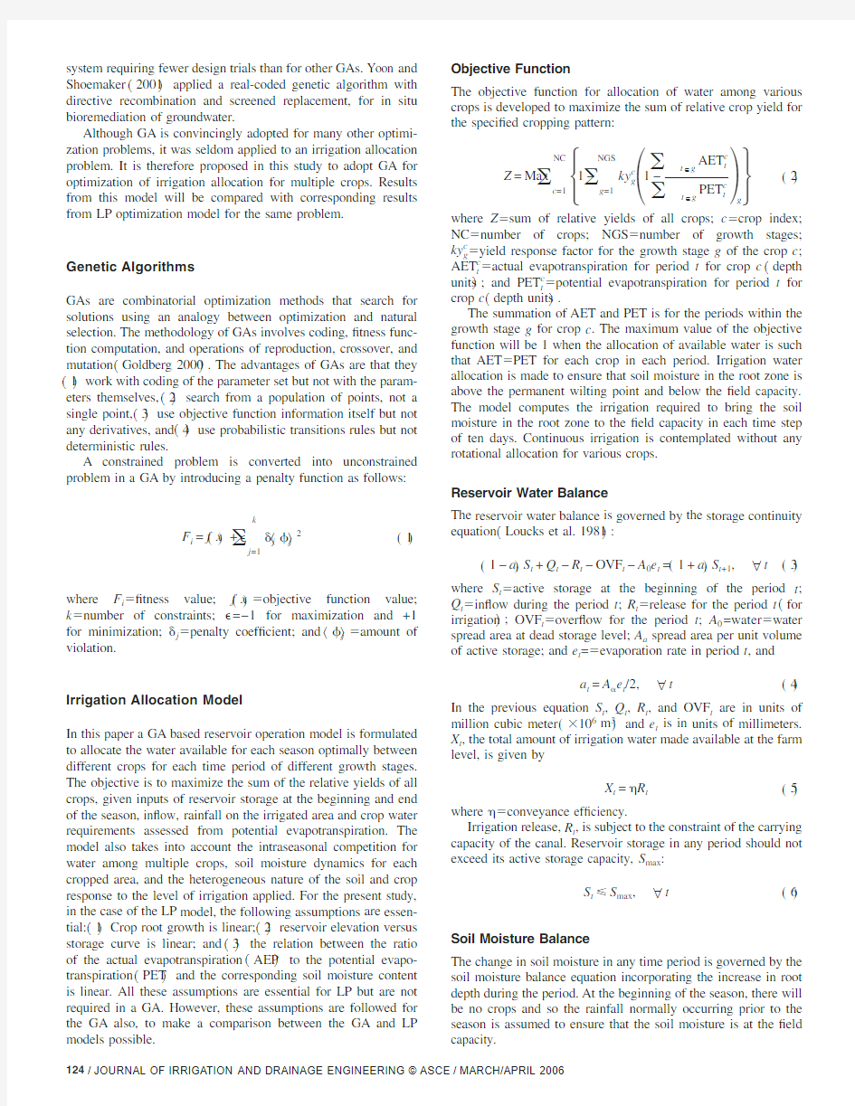
GAs are combinatorial optimization methods that search for solutions using an analogy between optimization and natural selection.The methodology of GAs involves coding,?tness func-tion computation,and operations of reproduction,crossover,and mutation ?Goldberg 2000?.The advantages of GAs are that they ?1?work with coding of the parameter set but not with the param-eters themselves,?2?search from a population of points,not a single point,?3?use objective function information itself but not any derivatives,and ?4?use probabilistic transitions rules but not deterministic rules.
A constrained problem is converted into unconstrained problem in a GA by introducing a penalty function as follows:
F i =f ?x ?+?
?j =1
k
?j ??j ?2?1?
where F i ??tness value;f ?x ??objective function value;k ?number of constraints;?=?1for maximization and +1for minimization;?j ?penalty coef?cient;and ??j ??amount of violation.
Irrigation Allocation Model
In this paper a GA based reservoir operation model is formulated to allocate the water available for each season optimally between different crops for each time period of different growth stages.The objective is to maximize the sum of the relative yields of all crops,given inputs of reservoir storage at the beginning and end of the season,in?ow,rainfall on the irrigated area and crop water requirements assessed from potential evapotranspiration.The model also takes into account the intraseasonal competition for water among multiple crops,soil moisture dynamics for each cropped area,and the heterogeneous nature of the soil and crop response to the level of irrigation applied.For the present study,in the case of the LP model,the following assumptions are essen-tial:?1?Crop root growth is linear;?2?reservoir elevation versus storage curve is linear;and ?3?the relation between the ratio of the actual evapotranspiration ?AEP ?to the potential evapo-transpiration ?PET ?and the corresponding soil moisture content is linear.All these assumptions are essential for LP but are not required in a GA.However,these assumptions are followed for the GA also,to make a comparison between the GA and LP models possible.
Objective Function
The objective function for allocation of water among various crops is developed to maximize the sum of relative crop yield for the speci?ed cropping pattern:
Z =Max
?c =1
NC
?
1?
?g =1
NGS
ky g
c ?
1?
?t ?g AET t c ?t ?g PET t
c ?g
?
?2?
where Z ?sum of relative yields of all crops;c ?crop index;NC ?number of crops;NGS ?number of growth stages;ky g c ?yield response factor for the growth stage g of the crop c ;AET t c ?actual evapotranspiration for period t for crop c ?depth units ?;and PET t c ?potential evapotranspiration for period t for crop c ?depth units ?.
The summation of AET and PET is for the periods within the growth stage g for crop c .The maximum value of the objective function will be 1when the allocation of available water is such that AET ?PET for each crop in each period.Irrigation water allocation is made to ensure that soil moisture in the root zone is above the permanent wilting point and below the ?eld capacity.The model computes the irrigation required to bring the soil moisture in the root zone to the ?eld capacity in each time step of ten days.Continuous irrigation is contemplated without any rotational allocation for various crops.Reservoir Water Balance
The reservoir water balance is governed by the storage continuity
equation ?Loucks et al.1981?:
?1?a t ?S t +Q t ?R t ?OVF t ?A 0e t =?1+a t ?S t +1,
?t
?3?
where S t ?active storage at the beginning of the period t ;Q t ?in?ow during the period t ;R t ?release for the period t ?for irrigation ?;OVF t ?over?ow for the period t ;A 0=water ?water spread area at dead storage level;A a spread area per unit volume of active storage;and e t =?evaporation rate in period t ,and
a t =A ?e t /2,
?t
?4?
In the previous equation S t ,Q t ,R t ,and OVF t are in units of million cubic meter ??106m 3?and e t is in units of millimeters.X t ,the total amount of irrigation water made available at the farm level,is given by
X t =?R t
?5?
where ??conveyance ef?ciency.
Irrigation release,R t ,is subject to the constraint of the carrying capacity of the canal.Reservoir storage in any period should not exceed its active storage capacity,S max :
S t ?S max ,
?t
?6?
Soil Moisture Balance
The change in soil moisture in any time period is governed by the soil moisture balance equation incorporating the increase in root depth during the period.At the beginning of the season,there will be no crops and so the rainfall normally occurring prior to the season is assumed to ensure that the soil moisture is at the ?eld capacity.
SM 1c =SM max c
,
?c ?7?
where SM 1c ?soil moisture above the permanent wilting point at
the beginning of the ?rst period ?t =1?for the crop c and SM max c ?soil moisture at the ?eld capacity for the crop c .It is assumed that the soil moisture is at the ?eld capacity in the incremental depth over which the crop root grows during each period.The soil moisture is expressed in depth units per unit root depth of the crop.The soil moisture balance equation for a given crop c for any period t is given by
SM t +1c D t +1c =SM t c D t c +IR t +x t c ?AET t c +SM max c
?D t +1c ?D t c ?
?DP t c ,
?c ,t ?8a ?
where SM t c ?available soil moisture at the beginning of the period t for the crop c ;D t c ?average root depth of crop c in period t ;IR t ?rainfall over irrigated area in period t ?depth units ?;x t c ?irrigation water allocated to crop c in period t ?depth units ?;and DP t c ?deep percolation during the period t for crop c .Deep percolation ?depth units ?,if any,can be computed as follows:
DP t c =?SM t c D t c +IR t +x t c ?AET t c ??SM max c
D t c ,
?c ,t ?8b ?
The available soil moisture in any period t for crop c cannot exceed the ?eld capacity
SM t
c ?SM max c ,
?c ,t
?9?
In general,AET remains the same as PET when the soil moisture is at ?eld capacity and also for a small fractional reduction from the ?eld capacity.However,to make the problem amenable for solution by LP,the reduction in soil moisture is assumed to be uniform right from the ?eld capacity to the permanent wilting point as done in earlier studies ?Vedula and Nagesh Kumar 1996?.The linear relationship between AET,PET,and the soil moisture ?between permanent wilting point and ?eld capacity ?is
AET t
c ?
SM t c D t c +IR t +x t
c
SM max c D t
c
PET t c ,
?c ,t ?10?
The upper bound for AET is PET:
AET t c ?PET t c ,
?c ,t ?11?
The heterogeneous nature of soils within the irrigated area can be
taken into account by modeling the soil moisture balance for each crop and soil type individually,i.e.,Eqs.?7?–?11?will be adapted for each soil type.Allocation Constraints
Irrigation water within a growth stage is provided uniformly among all the time periods of that growth stage to avoid undue concentrations ?Ashok 2002?:
x t
c =RG g c NP g
,?c ,t
except for t belonging to g =1
?12?
where RG g c ?irrigation allocation for the growth stage g of the crop c ?depth units ?;and NP g ?number of time periods in the growth stage g .
As the soil moisture is assumed to be at the ?eld capacity at the beginning of the ?rst time period,irrigation requirements will be nil during that period.In any period the total water allocated to all crops should be within the water available for allocation,X t .
?c
x t c AREA c
?X t ,?t ?13?
where AREA c ?area irrigated under crop c .For any growth stage
of any crop,the total allocation made should be equal to the sum of allocations made in all the periods of that growth stage
?t ?g
x t c =RG g c
,?c ,g ?14?
Irrigation water is not allocated to a crop for any period t ,which lies outside the growing season of that crop.This constraint is relevant,because all crops may not start at the same time and may not have the same duration.
The objective function given in Eq.?2?and the constraints in Eqs.?3?–?14?constitute the GA model which is implemented adopting binary code for the decision variables.The decision variable for the problem is x t c ,irrigation water allocated to crop c in period t in depth units.Binary string length for the decision variable,x t c ,is taken as 10bits ?decided based on the range of values for the variable ?separately for each crop for each time period.For example,in kharif season,when there are three crops and 15periods,with a string length 10bits each,there will be a total string length of 450bits.S t and SM t c are calculated for
each value of x t c
considering the in?ow,rainfall in the irrigated area,and potential evapotranspiration.It may be noted that the continuity equations for S t and SM t c ?Eqs.?3?and ?8??will be satis?ed due to the penalty function imposed on the continuity constraints of the model.
Case Study
The model has been applied to the right canal command area of the Malaprabha single-purpose irrigation reservoir in Karnataka State,India.The project is located at latitude 15°49?N and longitude 75°6?E.The catchment area of the river up to the dam site is 2,564km 2.The area of the reservoir at full reservoir level is 13,578ha.The reservoir has gross and live storage capacities of 1,070and 870?106m 3.The mean annual in?ow is 1,348.61?106m 3.The mean annual rainfall in the command area is 576mm.Fig.1shows the location map of the Malaprabha reservoir.There are two main canals under this project.The left bank canal serves a command area of 53,137ha and the right bank canal serves 1,286.34ha.As the left bank canal command is not fully developed irrigation was restricted to the right
bank
Fig.1.Location map of Malaprabha Reservoir
canal only.So the developed model is applied only to the right bank canal command.For this reservoir there are no mandatory downstream requirements.
The soil in a major portion of this command area is black cotton soil?Montmorrillonite,categorized as CH as per the uni?ed soil classi?cation system?and hence this soil type only was considered as was done in earlier studies?Vedula and Mujumdar1992;Vedula and Nagesh Kumar1996?.However, it may be noted that this is not a limitation of the model,as it can handle multiple soil types by considering each soil type individually by adapting Eqs.?7?–?11?for each soil type.
The farmers in this command area?with small holdings of less than20ha?are traditional and adopt a very similar cropping pattern every year.They do so to meet their own food require-ments and the decision is not commercially driven.Therefore the cropping pattern being adopted in the?eld,which is recurrent,is used in this model.Total crop water requirements used in this model were computed based on potential evapotranspiration. These requirements for the same area were evaluated earlier in previous studies by Vedula and Mujumdar?1992?and Vedula and Nagesh Kumar?1996?.
Results and Discussion
The water year?June–May?,is divided into36periods.There are two cropping seasons:kharif?Periods1–15?and rabi?Periods 16–31?.The last5periods of the year,that is,Periods31–36, will have no irrigation activity.The crops grown in the kharif season are sorghum,maize,and pulses and in rabi season wheat, sorghum,saf?ower,and pulses.The existing cropping pattern in the irrigated area showing principal crops,crop calendar, and the area irrigated during each season is presented in Fig.2.In addition,duration of each growth stage for each crop and the corresponding yield response factors?indicated in parentheses following each growth stage?are also shown therein.For this cropping pattern,the proposed model optimizes the allocation of the available water for each period from the reservoir.The values of A0and A a in the reservoir continuity equation?Eq.?3??are 37.01?106m2and0.117?106m2/m3,respectively.
The model was run with a crossover probability of0.8,a mutation probability of0.05and a population size of10.The maximum number of generations is?xed as20.The GA model is run for different in?ow and rainfall states at the beginning of the season.For this purpose,seasonal in?ow and rainfall variables are discretized into?ve discrete states based on statistical analysis of the available data?State1representing the lowest value and State 5representing the highest value?.These states represent various stages of the reservoir storage at the beginning of the season and the seasonal rainfall in the irrigated area.These states can as well represent various probabilities of exceedance of the respective variables.Seasonal values are disaggregated into corresponding values for ten day periods based on conditional expectations estimated using the historic data,i.e.,conditional probability of the ten day value in a particular class interval,given that the seasonal value is in a speci?ed state,is computed from the historic data for different class intervals and its expected value is then determined?Vedula and Nagesh Kumar1996?.
As indicated in the objective function and the subsequent explanation,when suf?cient water is available,it is allocated to all the crops to meet the crop water requirements.When there is de?cit supply,weightage is given to allocate irrigation water to the crops which are more sensitive to the de?cit condition. Weightages are decided based on the yield response factor?ky?for each crop for each growth stage given in Fig.2.For example, when there is a de?cit supply during Time Period6of the
kharif Fig.2.Crop calendar adopted in the command area
season,?rst priority will be given to maize ?with ky of 1.5?and next to sorghum ?ky ?0.55?and last to pulses ?ky ?0.35?in the proportion of ky values.It may be noted that such apportioning is done distributing de?cits over the entire crop season using the optimization model.
Fig.3presents variation of the relative yield of the maize crop in the kharif season and sorghum crop in rabi season ?when the in?ow and rainfall were highest,i.e.,in Discrete State 5?for different GA generations.GA model is solved for the remaining four discrete states of seasonal in?ow and seasonal rainfall.For lower values seasonal in?ow and seasonal rainfall states the yields are much lower and there is more stress for irrigation supplies.Optimal ten day releases for irrigation of each crop thus obtained for various discrete states of seasonal in?ow and seasonal rainfall constitute the derived operation policy for the reservoir.However,results corresponding to Discrete State 5only are presented for illustration.
AET values obtained with the GA allocation model are compared with those of a LP model in Fig.4for maize,pulses,and sorghum in kharif season.It is observed from Fig.4that AET values obtained by LP for maize are higher for irrigation allocation Periods 6,8,and 10whereas the values are practically the same for the remaining periods.Fig.5presents similar com-parison of AET values for sorghum,wheat,pulses,and saf?ower in rabi season.Signi?cant differences are observed in Periods 3and 7for sorghum;4and 8for pulses;3and 5for wheat;and 2for saf?ower.
It is observed from Figs.4and 5that AET values obtained by the GA and the LP compared well for most of the periods.The computational time required for the GA is practically insigni?cant compared to the time required for LP.For example for the kharif season,the computational time required for the GA is 50s whereas the LP required 180s on a Pentium III computer.Moreover the number of generations in the GA ?in this case 20?is not comparable to the number of iterations in the LP ?around 450for kharif season ?.In addition all the assumptions required for the LP model ?stated earlier ?are not required for the GA thus rendering the GA more realistic.
From this study,it is apparent that the GA performs well and is ef?cient when compared with LP.However,the LP model contains a very simple optimization approach due to the required but unrealistic simpli?cative hypotheses of linearity ?e.g.,the relation between AET/PET and the corresponding soil moisture
content is linear ?.The GA model proposed in this study can be further improved by incorporating nonlinear constraints to overcome the simpli?cations inherent in the LP model.
It is relevant to note that only one soil type was considered in the case study representing the predominant soil type in the irrigated area.However,in general,more than one soil type will be prevailing.As already indicated in the section on case study,this model can handle multiple soil types by adopting Eqs.?7?–?11?for each soil type.
Conclusions
An irrigation allocation model was developed to optimize relative yield from a speci?ed cropping pattern for various states of reservoir in?ows and rainfall in the irrigated area.The model integrates the reservoir releases with the consequent soil moisture at the root level for each crop and for each period.The model was applied to an existing single purpose reservoir in Karnataka State,India.In rabi season AET obtained is almost equal to PET indicating that optimal allocations were obtained from this model.It is observed that AET values obtained by GA and LP compared well.The operating policies evolved by the study can be adopted in the ?eld,for optimizing the utilization of the existing resources to obtain maximum
bene?ts.
Fig.3.Relative yield of maize in kharif season and sorghum in rabi season for different generations of GA for State
5
https://www.doczj.com/doc/3316738431.html,parison of AET values by GA and LP for kharif season
Notation
The following symbols are used in this paper:
A a ?water spread area per unit active storage volume;A 0?water spread area at dead storage level;AET t c ?actual evapotranspiration during period t for crop c
?depth units ?;AREA c
?area irrigated under crop c ;
a t ?variable that relates A a and e t ;c ?crop index;D t c ?average root depth of crop c in period t ;DP t c ?deep percolation during the period t for crop c ;e t ?evaporation rate in period t ;F i ??tness value;
f ?x ??objective function value;
IR t ?rainfall in period t ?depth units ?;k ?total number of constraints;ky g c ?yield response factor for growth stage g of crop c ;NC ?number of crops;
NGS ?number of growth stages;
NP g ?number of time periods in growth stage g ;
OVF t ?over?ow from the reservoir during the period t ;PET t c ?potential evapotranspiration during period t for crop
c ?depth units ?;
Q t ?in?ow into the reservoir during the period t ;R t ?release for irrigation from the reservoir for the
period t ;RG g c
?irrigation allocation for the growth stage g of the
crop c ?depth units ?;
S max ?maximum active storage capacity;
S t ?active storage at the beginning of the period t ;SM t c ?available soil moisture at the beginning of the
period t for the crop c ;SM max c
?available soil moisture at the ?eld capacity for the
crop c ;x t c
?irrigation water allocated to crop c in period t
?depth units ?;
X t ?total amount of irrigation water available at the
farm level;
?j ?penalty coef?cient;
???1for maximization ?+1for minimization ?;??conveyance ef?ciency;and ??j ??amount of violation.Subscripts
a ?active storage;c ?crop;
g ?growth stage;t ?time period;and 0?
dead storage.
References
Ashok, B.?2002?.“Optimal reservoir operation using genetic algorithms.”MTech dissertation,Indian Institute of Technology,Kharagpur,India.
Bras,R.L.,and Cordova,J.R.?1981?.“Intraseasonal water allocation in de?cit irrigation.”Water Resour.Res.,17?4?,866–874.
Dudley,N.J.,and Burt,O.R.?1973?.“Stochastic reservoir management and system design for irrigation.”Water Resour.Res.,9?3?,507–522.Goldberg,D.E.?2000?.Genetic algorithms in search,optimization and machine learning ,Addision-Wesley,Reading,Mass.
Hilton,A.B.C.,and Culver,T.B.?2000?.“Constraint handling for genetic algorithms in optimal remediation design.”J.Water Resour.Plan.Manage.,126?3?,128–137.
Loucks,D.P.,Stedinger,J.R.,and Haith,D.A.?1981?.Water resources systems planning and analysis ,Prentice-Hall,Englewood Cliffs,N.J.Mannocchi,F.,and Mecarelli,P.?1994?.“Optimization analysis of de?cit irrigation systems.”J.Irrig.Drain.Eng.,120?3?,484–503.
Morshed,J.,and Kaluarachchi,J.?2000?.“Enhancements to genetic algorithm for optimal ground-water management.”J.Hydrologic Eng.,5?1?,67–73.
Paul,S.,Panda,S.N.,and Nagesh Kumar,D.?2000?.“Optimal irrigation allocation:A multilevel approach.”J.Irrig.Drain.Eng.,126?3?
,
https://www.doczj.com/doc/3316738431.html,parison of AET values by GA and LP for rabi season
149–156.
Raju,K.S.,and Nagesh Kumar,D.?2004?.“Irrigation planning using genetic algorithms.”Water Resour.Manage.,18?2?,163–176. Reed,P.,Minsker, B.,and Goldberg, D. E.?2000?.“Designing
a competent simple genetic algorithm for search and optimization.”
Water Resour.Res.,36?12?,3757–3761.
Sharif,M.,and Wardlaw,R.?2000?.“Multireservoir systems optimization using genetic algorithms:Case study.”https://www.doczj.com/doc/3316738431.html,put.Civ.Eng.,14?4?, 255–263.
Vedula,S.,and Mujumdar,P.P.?1992?.“Optimal reservoir operation for irrigation of multiple crops.”Water Resour.Res.,28?1?,1–9. Vedula,S.,and Nagesh Kumar, D.?1996?.“An integrated model for optimal reservoir operation for irrigation of multiple crops.”Water
Resour.Res.,34?4?,1101–1108.
Wardlaw,R.,and Barnes,J.?1999?.“Optimal allocation of irrigation water supplies in real time.”J.Irrig.Drain.Eng.,125?6?,345–354. Wardlaw,R.,and Sharif,M.?1999?.“Evaluation of genetic algorithms for optimal reservoir system operation.”J.Water Resour.Plan.Manage., 125?1?,25–33.
Wu,Z.Y.,and Simpson,A.R.?2001?.“Competent genetic-evolutionary optimization of water distribution systems.”https://www.doczj.com/doc/3316738431.html,put.Civ.Eng., 15?2?,89–101.
Yoon,J.H.,and Shoemaker,C.A.?2001?.“An improved real-coded GA for groundwater bioremediation.”https://www.doczj.com/doc/3316738431.html,put.Civ.Eng.,15?3?, 224–231.
贷款利息的计算公式 公式 1、短期贷款利息的计算 短期贷款(期限在一年以下,含一年),按贷款合同签定日的相应档次的法定贷款利率计息。贷款 合同期内,遇利率调整不分段计息。 短期贷款按季结息的,每季度末月的20日为结息日;按月结息的,每月的20日为结息日。具体 结息方式由借贷双方协商确定。对贷款期内不能按期支付的利息按贷款合同利率按季或按月计收复利,贷款逾期后改按罚息利率计收复利。最后一笔贷款清偿时,利随本清。 2、中长期贷款利息的计算 中长期贷款(期限在一年以上)利率实行一年一定。贷款(包括贷款合同生效日起一年内应分笔 拨付的所有资金)根据贷款合同确定的期限,按贷款合同生效日相应档次的法定贷款利率计息,每满一年后(分笔拨付的以第一笔贷款的发放日为准),再按当时相应档次的法定贷款利率确定下一年度利 率。 中长期贷款按季结息,每季度末月二十日为结息日。对贷款期内不能按期支付的利息按合同利率按季计收复利,贷款逾期后改按罚息利率计收复利。 3、贴现按贴现日确定的贴现利率一次性收取利息 4、贷款展期,期限累计计算,累计期限达到新的利率期限档次时,自展期之日起,按展期日挂牌的同档次利率计息;达不到新的期限档次时,按展期日的原档次利率计息。 5、逾期贷款或挤占挪用贷款,从逾期或挤占挪用之日起,按罚息利率计收罚息,直到清偿本息为止, 遇罚息利率调整分段计息。对贷款逾期或挪用期间不能按期支付的利息按罚息利率按季(短期贷款也 可按月)计收复利。如同一笔贷款既逾期又挤占挪用,应择其重,不能并处。 6、借款人在借款合同到期日之前归还借款时,贷款人有权按原贷款合同向借款人收取利息。 (二)贷款利息的计算 1. 定期结息的计息方法 定期结息是指银行在每月或每季度末月20日营业终了时,根据贷款科目余额表计算累计贷款积数 (贷款积数计算方法与存款积数计息方法相同),登记贷款计息科目积数表,按规定的利率计算利息。 定期结息的计息天数按日历天数,有一天算一天,全年按365天或366天计算。算头不算尾,即从贷
1、某客户2011年8月1日贷款10000元,到期日为2012 年6月20日,利率7.2‰,该户于2012年5月31日前来还款,计算贷款利息应收多少? 304*7.2‰*10000/30=729.6(元) 2、2012年7月14日,某客户持一张2012年5月20日签 发、到期日为2012年10月31日、金额10万元的银行承兑汇票,到我行办理贴现,已知贴现率为4.5‰,我行规定加收邮程为3天,计算票据办理贴现后实际转入该客户账户金额是多少? 答:贴现天数为109天,另加3天邮程共112天 利息收入:100000*112*4.5‰/30=1680 实际转入该客户账户100000-1680=98320 重点在于天数有天算一天,大月31日要加上,另3天邮程要加上 3、张三2012年1月1日在我行贷款5000元,到期日为 2012年10月20日,利率9‰,利随本清,约定逾期按15‰罚息,张三于2012年12月10日还款,他共要支付多少利息? 答:期限内天数293天,293*5000*9‰/30=439.50 逾期51天,51*5000*15‰/30=127.50 439.50+127.50=567元
4、张三2011年1月1日在我行贷款10000元,到期日为 2011年12月31日,利率7.2‰,利随本清,约定逾期按12‰计算罚息,张三于2011年9月1日要求先行归还部分贷款,本金加利息共计5000元,计算本金和利息各是多少? 答:归还时天数为243天, 本金=5000÷(1+7.2‰÷30×243)=4724.47 利息=275.53 5、如上题,张三在2011年9月1日归还部分贷款后,直 到2012年4月10日才来还清贷款,计算他应支付本息共计多少? 答:本金=10000-4724.47=5275.53 期限内天数=364天逾期天数=101天 5275.53×7.2‰÷30×364+5275.53×12‰÷30×101 =460.87+213.13 =674元(利息) 本息合计5275.53+674=5949.53
调整时间六个月 以内 (含六 个月) 六个月 至一年 (含一 年) 一至 三年 (含 三年) 三至五 年(含五 年) 五年 以上 欠款本 金(假设 X) 年利率 (%) 年 天 数 期间 天数 利息 1991.04.21-1993.05.148.108.649.009.549.72X 9.00% 360 754 1993.05.15-1993.07.108.829.3610.8012.0612.24X 8.82% 360 56 1993.07.11-1994.12.319.0010.9812.2413.8614.04X 12.24% 360 538 1995.01.01-1995.06.309.0010.9812.9614.5814.76X 10.98%360 180 1995.07.01-1996.04.3010.0812.0613.5015.1215.30X 12.06% 360 304 1996.05.01-1996.08.229.7210.9813.1414.9415.12X 9.72% 360 113 1996.08.23-1997.10.229.1810.0810.9811.7012.42X 10.98% 360 425 1997.10.23-1998.03.247.658.649.369.9010.53X 7.65% 360 152 1998.03.25-1998.06.307.027.929.009.7210.35X 7.02% 360 97 1998.07.01-1998.12.06 6.57 6.937.117.658.01X 6.57% 360 158 1998.12.07-1999.06.09 6.12 6.39 6.667.207.56X 6.39% 360 184 1999.06.10-2002.02.20 5.58 5.85 5.94 6.03 6.21X 5.94% 360 986 2002.02.21-2004.10.28 5.04 5.31 5.49 5.58 5.76X 5.49% 360 980 2004.10.29-2006.04.27 5.22 5.58 5.76 5.85 6.12X 5.76% 360 545 2006.04.28-2006.08.18 5.40 5.85 6.03 6.12 6.39X 5.40% 360 112 2006.08.19-2007.03.17 5.58 6.12 6.30 6.48 6.84X 6.12% 360 210 2007.03.18-2007.05.18 5.67 6.39 6.57 6.757.11X 5.67% 360 61 2007.05.19-2007.07.20 5.85 6.57 6.75 6.937.20X 5.85% 360 62 2007.07.21-2007.08.21 6.03 6.847.027.207.38X 6.03% 360 31 2007.08.22-2007.09.14 6.217.027.207.387.56X 6.21% 360 23 2007.09.15-2007.12.20 6.487.297.477.657.83X 6.48% 360 96 2007.12.21-2008.09.15 6.577.477.567.747.83X 7.47% 360 269 2008.09.16-2008.10.08 6.217.207.297.567.74X 6.21% 360 22
贷款利息计算法则概要 【说明】根据不良资产操作的实践需要,整理本概要。概要主要分为五个部分: 一、利息计算的基本常识………………………………………………1-2 二、合同期限内的利息计算……………………………………………2-3 三、合同逾期后的利息计算……………………………………………3-4 四、逾期违约金的计算…………………………………………………4-5 五、迟延履行期间的债务利息(双倍利息)的计算…………………5-6 每一部分主要由计算常/变量(主要是利率的确定)、计算公式(基本相同)和计算依据(央行规定及司法解释)三部分组成,争取做到简介明了、有理有据。对尚未找到明确依据的问题,笔者的意见仅供参考,具体见下文。 一、利息计算的基本常识 (一)人民币业务的利率换算公式为(注:存贷通用): 1.日利率(0/000)=年利率(%)÷360=月利率(‰)÷30 2.月利率(‰)=年利率(%)÷12 (二)银行可采用积数计息法和逐笔计息法计算利息。 1.积数计息法按实际天数每日累计账户余额,以累计积数乘以日利率计算利息。计息公式为: 利息=累计计息积数×日利率,其中累计计息积数=每日余额合计数。 2.逐笔计息法按预先确定的计息公式利息=本金×利率×贷款期限逐笔计算利息,具体有三: 计息期为整年(月)的,计息公式为: ①利息=本金×年(月)数×年(月)利率 计息期有整年(月)又有零头天数的,计息公式为: ②利息=本金×年(月)数×年(月)利率+本金×零头天数×日利率 同时,银行可选择将计息期全部化为实际天数计算利息,即每年为365天(闰年366天),每月为当月公历实际天数,计息公式为: ③利息=本金×实际天数×日利率 这三个计算公式实质相同,但由于利率换算中一年只作360天,但实际按日利率计算时,一年将作365天计算,得出的结果会稍有偏差。具体采用那一个公式计算,央行赋予了金融机构自主选择的权利。因此,当事人和金融机构可以就此在合同中约定。表一是各商业银行的通常做法。 (表一) 序号项目名称计息方法 1 公司贷款逐笔计息法(公式③) 2 贸易融资逐笔计息法(公式③) 3 零售贷款 4 等额本金还款法逐笔计息法(公式②)
工商银行贷款利率计算方法 一、短期贷款 六个月(含)5.35% 六个月至一年(含)5.81% 二、中长期贷款 一至三年(含)5.85% 三至五年(含)6.22% 五年以上6.40% 三、贴现 以20万20年首套房贷为例: 银行贷款利率是根据贷款的信用情况等综合评价的,根据信用情况、抵押物、国家政策(是否首套房)等来确定贷款利率水平,如果各方面评价良好,不同银行执行的房贷利率有所差别,2011年由于资金紧张等原因,部分银行首套房贷款利率执行基准利率的1.1倍或1.05倍。 从2012年开始,多数银行将首套房利率调整至基准利率。4月上旬,国有大银行开始执行首套房贷利率优惠。部分银行利率最大优惠可达85折。现行基准利率是2011年7月7日调整并实施的,利率为五年期以上7.05%,优惠后月利率为7.05%*0.85/12 20万20年(240个月)月还款 额:200000*7.05%*0.85/12*(1+7.05%*0.85/12)^240/[(1+7.05%*0.8 5/12)^240-1]=1432.00元 利息总额:1432.00*240-200000=143680
说明:^240为240次方 按照货币资金借贷关系持续期间内利率水平是否变动来划分,贷款利率可分为固定利率与浮动利率。浮动利率是指在借贷期限内利 率随物价或其他因素变化相应调整的利率。借贷双方可以在签订借 款协议时就规定利率可以随物价或其他市场利率等因素进行调整。 浮动利率可避免固定利率的某些弊端,但计算依据多样,手续繁杂。 利率按市场利率的变动可以随时调整。常常采用基本利率加成计算。通常将市场上信誉最好企业的借款利率或商业票据利率定为基 本利率,并在此基础上加0.5至2个百分点作为浮动利率。到期按 面值还本,平时按规定的付息期采用浮动利率付息。 浮动利率的特点: 1、利率的变动可以灵敏地反映金融市场上资金的供求状况; 2、借贷双方所承担的利率变动的风险较小; 3、便于金融机构及时根据市场利率的变动情况调整其资产负债 规模; 4、有助于中央银行及时了解货币政策的效果并做出相应的政策 调整。 固定利率与浮动利率的优缺点: 固定利率与浮动利率各有其优缺点。固定利率便于借方计算成本,浮动利率可以减少市场变化的风险,但不便于计算与预测收益和成本。 根据贷款期限贷款利率可分为长期贷款利率和短期贷款利率 各种中长期贷款利率等,是资本市场的利率。 贷款利率政策是我国信贷政策的一个重要组成部分,利率是国家调节经济活动的一个重要杠杆。 (1)法定贷款利率法定贷款利率是指经国务院批准和国务院授权 中国人民银行制定的各种贷款利率。法定贷款利率一经确定,任何
贷款利率 百科名片 贷款利率 贷款利率,是指借款期限内利息数额与本金额的比例。我国的利率由中国人民银行统一管理,中国人民银行确定的利率经国务院批准后执行。贷款利率的高低直接决定着利润在借款企业和银行之间的分配比例,因而影响着借贷双方的经济利益。贷款利率因贷款种类和期限的不同而不同,同时也与借贷资金的稀缺程度相联系。 目录 定义 最新人民币贷款利率 历年人民币贷款利率变动表 贷款利率还款表 分类 长期贷款利率和短期贷款利率 理论争议 1相关贷款利率知识1.什么是法定利率? 12.什么是基准利率? 13.什么是合同利率? 14.贷款利率应如何确定?贷款利息如何计收? 15.贷款结息如何规定? 16.贷款法定利率调整 17.贷款期限内不能按约定支付利息的 18.约期内贷款利率如何调整? 19.如果贷款展期则贷款的利率应如何确定? 110.挤占挪用和逾期贷款的加罚息 贷款利率管理政策 贷款利率浮动范围 展开 定义 贷款利率是借款合同双方当事人计算借款利息的主要依据,贷款利率条款是借款
合同的主要条款。以银行等金融机构为出借人的借款合同的利率的确定,当事人只能在中国人民银行规定的利率上下限范围内进行协商。如果当事人约定的贷款利率高于中国人民银行规定利率的上限,则超出部分无效;如果当事人约定的利率低于中国人民银行规定的利率下限,应当以中国人民银行规定的最低利率为准。此外,如果贷款人违反了中国人民银行规定,在计收利息之外收取任何其他费用的,应当由中国人民银行进行处罚。银行利率的一种,一般情况下比存款利率高,两者之差是银行利润的主要来源。 最新人民币贷款利率 单位:年利率% 项目2011-2-9调整后利率 一、各项商业贷款 六个月以内(含) 5.60 六个月至一年(含) 6.06 一至三年(含) 6.10 三至五年(含) 6.45 五年以上 6.60 贴现以再贴现利率为下限加点确定 二、个人住房公积金贷款2011-2-9调整后利率 五年以下(含五年) 4.00 五年以上 4.50 注:中国人民银行决定,自2011年2月9日起上调金融机构人民币存贷款基准利率。历年人民币贷款利率变动表 以下是从1991年以来中国央行公布的历年贷存款利率表,也可以去查看历年存款利率表。金融机构人民币贷款基准利率 调整时间六个月以 内 (含六个 月) 六个月至 一年 (含一 年) 一至三 年 (含三 年) 三至五 年 (含五 年) 五年以上 1991.0 4.21 8.10 8.64 9.00 9.54 9.72 1993.0 5.15 8.82 9.36 10.80 12.06 12.24 1993.09.00 10.98 12.24 13.86 14.04
工商银行贷款利率计算方法 工商银行贷款利率计算方法 一、短期贷款 六个月(含) 5.35% 六个月至一年(含) 5.81% 二、中长期贷款 一至三年(含) 5.85% 三至五年(含) 6.22 % 五年以上6.40% 三、贴现 以20万20年首套房贷为例: 银行贷款利率是根据贷款的信用情况等综合评价的,根据信用情况、抵押物、国家政策(是否首套房)等来确定贷款利率水平,如果各方面评价良好,不同银行执行的房贷利率有所差别,2011年由于资金紧张等原因,部分银行首套房贷款利率执行基准利率的1.1倍或1.05倍。
从2012年开始,多数银行将首套房利率调整至基准利率。4月上旬,国有大银行开始执行首套房贷利率优惠。部分银行利率最大优惠可达85折。现行基准利率是2011年7月7日调整并实施的,利率为五年期以上7.05%,优惠后月利率为7.05%*0.85/12 20万20年(240个月)月还款额: 200000*7.05%*0.85/12*(1+7.05%*0.85/12)?/[(1+7.05%*0.85/12)?-1]=1432.00元 利息总额:1432.00*240-200000=143680 说明:?为240次方 工商银行贷款利率相关分类 按照货币资金借贷关系持续期间内利率水平是否变动来划分,贷款利率可分为固定利率与浮动利率。浮动利率是指在借贷期限内利率随物价或其他因素变化相应调整的利率。借贷双方可以在签订借款协议时就规定利率可以随物价或其他市场利率等因素进行调整。浮动利率可避免固定利率的某些弊端,但计算依据多样,手续繁杂。 中国曾一度实行过的对中长期储蓄存款实行保值贴补的办法就是浮动利率制的一种形式。 利率按市场利率的变动可以随时调整。常常采用基本利率加成
银行贷款利息怎么计算 笼统的说都是贷款本金×期限×利率。比如个人按揭贷款,按月还款,就是贷款剩余本金×月利率×1(1个月)。 举例来说:100万贷款,10年期,年利率6.8%。 首先把年利率换算成月利率=6.8%/12=0.566667%。 如果是等本金还款,那么第一个月的利息是1000000×0.566667%=5666.67元。每个月要还的本金是1000000/120=8333.33元,合计14000元。第二个月要还的利息就是(1000000-8333.33)×0.566667%=5619.45元,依此类推,每月利息可以少还47.22元。 如果是等本息还款,那么计算就比较复杂了。 首先计算出来的是每个月要还的金额是11508.03。公式是1000000×0.566667%×(1+0.566667%)120/[(1+0.566667%)120-1]。这样第一个月要还的利息不变还是5666.67,但第一个月还的本金是11508.03-5666.67=5841.36。第二个月要还的利息就是(1000000-5841.36)×0.566667%=5633.57元。第二个月要还的本金是11508.03-5633.57=5874.46元。 从上边的计算也可以看出来,等本金法还款,开始时候的每月还款要高于等本息法,但从第二个月开始,要还的利息就少于等本息法,这样10年算下来利息要比等本息法少不少。 等额本息计算公式:月还款金额=〔贷款本金×月利率×(1+月利率)还款月数〕/〔(1+月利率)还款月数-1〕 等额本金计算公式:月还款金额= (贷款本金/还款月数)+(本金- 已归还本金累计额)×每月利率 举例说明:假设以10000元为本金、在银行贷款10年、基准利率是6.65%,比较下两种贷款方式的差异。 等额本息还款法: 月利率=年利率÷12=0.0665÷12=0.005541667 。月还款本息=〔10000×0.005541667×(1+0.005541667)120〕÷〔(1+0.005541667)120-1〕=114.3127元。合计还款13717.52元;合计利息3717.52万元。 等额本金还款法: 每月还款金额= (贷款本金÷还款月数)+(本金- 已归还本金累计额)×每月利率=(10000 ÷120)+(10000- 已归还本金累计额)×0.005541667。首月还款138.75元每月递减0.462元,合计还款13352.71元;利息3352.71元。
工商银行贷款利息计算 贷款利息,是指贷款人因为发出货币资金而从借款人手中获得的报酬,也是借款人使用资金必须支付的代价。下面让来告诉你工商银行贷款利息计算,希望能帮到你。 工商银行贷款利息计算当月贷款利息=上月剩余本金*贷款月利率; 当月已还本金=当月还款额-当月贷款利息; 上月剩余本金=贷款总额-累计已还本金。 工商银行贷款利息的定义贷款利息,是指贷款人因为发出货币资金而从借款人手中获得的报酬,也是借款人使用资金必须支付的代价。银行贷款利率是指借款期限内利息数额与本金额的比例。以银行等金融机构为出借人的借款合同的利率确定,当事人只能在中国银行规定的利率上下限的范围内进行协商。贷款利率高,则借款期限后借款方还款金额提高,反之,则降低。决定贷款利息的三大因素:贷款金额、贷款期限、贷款利率。 工商银行贷款利息的计算方式(一)人民币业务的利率换算公式为(注:存贷通用): 1.日利率(0/000)=年利率(%)÷360=月利率(‰)÷30 2.月利率(‰)=年利率(%)÷12
(二)银行可采用积数计息法和逐笔计息法计算利息。 1.积数计息法按实际天数每日累计账户余额,以累计积数乘以日利率计算利息。计息公式为: 利息=累计计息积数×日利率,其中累计计息积数=每日余额合计数。 2.逐笔计息法按预先确定的计息公式利息=本金×利率×贷款期限逐笔计算利息,具体有三: 计息期为整年(月)的,计息公式为: ①利息=本金×年(月)数×年(月)利率 计息期有整年(月)又有零头天数的,计息公式为: ②利息=本金×年(月)数×年(月)利率+本金×零头天数×日利率 同时,银行可选择将计息期全部化为实际天数计算利息,即每年为365天(闰年366天),每月为当月公历实际天数,计息公式为: ③利息=本金×实际天数×日利率 这三个计算公式实质相同,但由于利率换算中一年只作360天,但实际按日利率计算时,一年将作365天计算,得出的结果会稍有偏差。具体采用那一个公式计算,央行赋予了金融机构自主选择的权利。因此,当事人和金融机构可以就此在合同中约定。 (三)复利:复利即对利息按一定的利率加收利息。按照央行的规定,借款方未按照合同约定的时间偿还利息的,就要加收复利。 (四)罚息:贷款人未按规定期限归还银行贷款,银行按与当事人签
银行贷款利息是怎么样计算的 一、短期贷款六个月(含) 5、58六个月至一年(含) 6、12 二、中长期贷款一至三年(含) 6、30三至五年(含) 6、48以下简单说四个例子,希望对您有帮助。第一,银行活期存款利息怎算?已知在银行有一笔固定的定期存款总额M、年利率是r 。银行每年将支付利息I=M*r 。如果这家银行是每半年结算一次利息,那麼每次的利息是I=M*r/2 。因为计算简单,我就不举数字计算例了。第二,银行定存利息怎算? 1、如果跟银行约定的是一年期整存整取的定存,那麼银行在您存满一年之后将支付本金加利息P+I=M*(1+r/12)^12 。本金P 就是原始存款总额M。利息就是I=M*(1+r/12)^121)/(r/12) 3、解式1与式2,得Po+Io即等额本息金额Po+Io = [M * (1+r/12)^N]/[(((1+r/12)^N)-1)/(r/12)] 4、举例,贷款总额M=5,000,000,贷款20年总期数N=2 40、利率r = 4、5%,代入第3式,得等额本息值Po+Io =31,6 32、47 ,其中第1个月还本Po=128 82、47第1个月付息Io=18750第2个月还本Po=129
30、78第2个月付息Io=18701、69第3个月还本Po=129 79、27第3个月付息Io=186 53、2第4个月还本Po=130 27、94第4个月付息Io=18604、53(以下类推)第240个月还本Po=315 14、29第240个月付息Io=1 18、1786计算关键在先以第3式算出等额本息值Po+Io再在每个月先求出利息It=前期未还本金*r/12再算出每个月还本金额Pt=(Po+Io)-当月利息It目前银行整存整取,一年期年利率 2、52 %,例如存1000元一年期整存整取,利息1000× 2、52 %= 25、2元,利息税20%, 25、2×20%= 5、04元,一年后可以取出1000+( 25、2- 5、04)=10 20、16元,实际的获得利息为 20、16元
按银行同期贷款利率怎么计算? 如今,大多数借款人都有急需用钱的时候,相信大家都会选择在银行贷款,因为在银行贷款比较安全可靠,在申办贷款时,银行基准利率是大家比较关心的问题,因为银行基准利率直接关系到大家的还款额度。那么问题来了,按银行同期贷款利率怎么计算?你们了解吗?接下来,请跟随贷上我小编来看看吧。 据小编的了解,最新银行贷款基准利率如下: 贷款期限为:六个月以内(含6个月),则贷款利率为5.60%; 贷款期限为:六个月至1年(含1年),则贷款利率为6.00%; 贷款期限为:一年至三年(含3年),则贷款利率为6.15%; 贷款期限为:三年至五年(含5年),则贷款利率为6.40%; 贷款期限为:五年以上,则贷款利率为6.55%; 相信大家都知道目前最主要的还款方式包括有:等额本息、等额本金。选择不同的还款方式,所产生的利息也不一样。 等额本息计算公式为:〔贷款本金×月利率×(1+月利率)^还款月数〕÷〔(1+月利率)^还款月数-1〕 等额本金计算公式如下: 每月还款金额为:(贷款本金÷还款月数)+(本金—已归还本金累计额)×每月利率(其中^符号表示乘方) 由此可看,当申请人在申办贷款的时候,小编建议借款人应前往当地银行或者是贷款机构咨询了解下。 听了上述贷上我小编的详细解答后,相信大家对于按银行同期贷款利率怎么计算也有了一定的了解了,大家可以针对以上事项做好相应的准备,这样才能更加顺利的办理到贷款,希望小编的介绍可以给有需要的人提供一些帮助。 第 1 页共1 页 以凡注明“贷上我”来源之作品,任何媒体和个人全部或者部分转载,请注明出处(贷上我https://www.doczj.com/doc/3316738431.html,)。