SUPPORTING INFORMATION
Altitudinal and Spatial Signature of Persistent Organic Pollutants in Soil, Lichen, Conifer Needles and Bark of the Southeast Tibetan Plateau: Implications for Sources and Environmental Cycling Ruiqiang Yang a, Shujuan Zhang a, An Li b, Guibin Jiang a, Chuanyong Jing a*
a: State Key Laboratory of Environmental Chemistry and Ecotoxicology, Research Center for Eco-Environmental Sciences, Chinese Academy of Sciences, P.O. Box 2871, Beijing, 100085, China
b: School of Public Health, University of Illinois at Chicago, Chicago, Illinois 60612, United States
* E-mail: cyjing@https://www.doczj.com/doc/2413681436.html,
Table of Content
(In the order of mention in the main text)
Text S1 Detailed information of sample analysis.S2-3 Table S1 Description of the sampling sites and selected information.S4-5 Table S2 Chemicals, abbreviations, and related properties. S6 Table S3 The statistical concentrations of PAHs and OCPs in the four matrices (ng/g dw).S7 Table S4 Comparison of PAH and OCP concentrations (ng/g) with other remote areas.S8
Figure S1 Altitudinal trend of the logarithm concentrations for PAHs and OCPs along the transects.
S9-10
Table S5 Statistics of linear regression between Log transformed concentration (ng/g, y)
and altitude (x=altitude/104) in the four matrices.
S11-
13
Table S6 Summary of the altitudinal gradient (slopes). S13-14
Table S7 Comparision of linear regression coefficients (R2) in concentraion and altitude between dry weight basis and TOC/lipid basis in transects 3 and 4.
S14
Figure S2 The linear correlation between TOC and PAH concentrations.S15 Figure S3 Correlation of conifer tree bark lipid with altitude. S16
Table S8 Correlation coefficients of PAH and OCP log-transformed concentrations on dry weight basis (lower triangular) and lipid weight basis (upper triangular)
between the four matrices (N=24).
S17
Figure S4 Concentrations of PAHs and OCPs versus depth in soil core from forest site and clearing site
S18
Figure S5 Monthly average surface wind vector field of the southeast Tibet. A: July and B: January in 2010.
S18
Figure S6 Bivariate plot for diagnostic ratios of PAHs. S19 Table S9 Ranges of α-/γ-HCH, o,p’-/p,p’-DDT and DDT/DDE in the four matrices.S20 Table S10 The linear correlation of α-/γ-HCH verse altitude along the transects. S20 References S20-
21
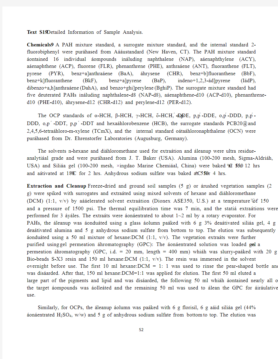
Text S1. Detailed Information of Sample Analysis.
Chemicals. A PAH mixture standard, a surrogate mixture standard, and the internal standard 2-fluorobiphenyl were purchased from Accustandard (New Haven, CT). The PAH mixture standard contained 16 individual compounds including naphthalene (NAP), acenaphthylene (ACY), acenaphthene (ACP), fluorene (FLR), phenanthrene (PHE), anthracene (ANT), fluoranthene (FLT), pyrene (PYR), benz[a]anthracene (BaA), chrysene (CHR), benz[b]fluoranthene (BbF), benz[k]fluoranthene (BkF), benz[a]pyrene (BaP), indeno[1,2,3-cd]pyrene (IcdP), dibenzo[a,h]anthracene (DahA), and benzo[ghi]perylene (BghiP). The surrogate mixture standard had five deuterated PAHs including naphthalene-d8 (NAP-d8), acenaphthene-d10 (ACP-d10), phenanthrene-
d10 (PHE-d10), chrysene-d12 (CHR-d12) and perylene-d12 (PER-d12).
The OCP standards of α-HCH, β-HCH, γ-HCH, δ-HCH, o,p′-DDE, p,p′-DDE, o,p′-DDD, p,p′-DDD, o,p′-DDT, p,p′-DDT and hexachlorobenzene (HCB), the surrogate standards PCB209 and 2,4,5,6-tetrachloro-m-xylene (TCmX), and the internal standard octachloronaphthalene (OCN) were purchased from Dr. Ehrenstorfer Laboratories (Augusburg, Germany).
The solvents n-hexane and dichloromethane used for extraction and cleanup were ultra residue-analytical grade and were purchased from J. T. Baker (USA). Alumina (100-200 mesh, Sigma-Aldrich, USA) and Silica gel (100-200 mesh, Qingdao Marine Chemical, China) were baked at 550°C for 12 hrs and activated at 180°C for 2 hrs. Anhydrous sodium sulfate was baked at 550°C for 4 hrs.
Extraction and Cleanup. Freeze-dried and ground soil samples (5 g) or crushed vegetation samples (2 g) were spiked with surrogates and extracted using mixed solvents of hexane and dichloromethane (DCM) (1:1, v/v) by accelerated solvent extraction (Dionex ASE350, U.S.) at a temperature of 150℃and a pressure of 1500 psi. The thermal equilibration time was 7 min, and the static extractions were performed for 3 cycles. The extracts were concentrated to about 1~2 ml by a rotary evaporator. For PAHs, the cleanup was conducted using a glass column packed with 6 g 3% deactivated silica gel, 4 g 2% deactivated alumina and 5 g anhydrous sodium sulfate from bottom to top. The elution was subsequently conducted using a 50 ml mixture of hexane:DCM (1:1, v/v). The vegetation extracts were further purified using gel permeation chromatography (GPC): The concentrated solution was loaded on a gel permeation chromatography (GPC, i.d. = 20 mm, length = 400 mm) which was slurry-packed with 20 g Bio-beads S-X3 resin and 150 ml hexane:DCM (1:1, v/v). The resin was immersed in the solvent overnight before use. The first 10 ml hexane:DCM = 1: 1 was used to rinse the pear-shaped bottle and was discarded. After that, 150 ml hexane:DCM=1:1 was applied for elution. The first 50 ml eluted a large part of the pigments and lipid and was discarded, the following 50 ml which contained nearly all of the target compounds was collected and the remaining 50 ml was used to clean the GPC for circulative use.
Similarly, for OCPs, the cleanup column was packed with 6 g florisil, 6 g acid silica gel (44% concentrated H2SO4, w/w) and 5 g of anhydrous sodium sulfate from bottom to top. The elution was
subsequently conducted using 10 ml hexane and a 50 ml mixture of hexane and dichloromethane (4:1, v/v). The elutes were concentrated to a final 0.5 ml by rotary evaporation and a high-purity nitrogen stream. The internal standards OCN (for OCPs) and 2-fluorobiphenyl (for PAHs) were added before injection.
Instrumental Analysis. An Agilent-7890 gas chromatograph (GC) equipped with a HP-5 MS capillary column (30 m × 0.25 mm i.d. × 0.25 um film thickness) was used to separate PAHs while a mass spectrometer (MS, Agilent 5975) with electron ionization (EI) was used to analyze PAHs. The oven temperature program was operated as follows: initial 60°C for 2 min, 6°C /min to 300°C, and held for a final 10 min. The temperature of the injector was set at 280°C. Two microliters of the extracts were injected in the pulsed splitless mode. High-purity helium was used as the carrier gas with a constant flow of 1 ml/min. The MS detector was operated at 70 eV and the ion source was set at 300°C. The quadruple and interface temperatures were 180°C and 300°C, respectively. The MS detector was operated in selected ion monitoring (SIM) mode.
For OCP analysis, an Agilent-7890 GC equipped with a 63Ni electron capture detector (micro-ECD) was used. The samples were analyzed using two capillary columns with different polarity (HP-5 and DB-1701). Both columns were 30 m long and had a 0.25 mm i.d. and a 0.25 um stationary phase film thickness. The temperatures of the injector and detector were set at 250°C and 350°C, respectively. Two microliters of the extracts were injected in the pulsed splitless mode. High-purity Helium was used as the carrier gas with a constant flow of 1 ml/min, and high-purity nitrogen was used as the make-up gas and controlled at 59 ml/min. The oven temperature program was 80°C held for 1 min, ramped at 15°C / min to 140°C, held for 1 min, and then at 5°C /min to 230°C, held for 4 min, and finally at 25°C /min to 300°C, held for 2 min.
A procedural blank was run every set of 10 samples. The dominant PAH congener was NAP in the procedural blanks, and the mean concentration was 6.1 ng/g, which was much lower compared with the levels in the samples. The dominant OCPs were HC
B and α-HCH in the procedural blanks, and the mean concentrations were 0.026 ng/g and 0.025 ng/g, respectively, which were significantly lower than the levels for most of the samples. All the concentrations reported in this paper were after subtraction of the procedural blank levels and corrected based on the recoveries of the surrogates.
Table S1. Description of the sampling sites and related information.
Transect ID Latitude (°N) Longitude (°E) Altitude (m)
TOC or lipid content (%) Soil Needle Bark Lichen
1 1 29.6377 91.2009 3668 1.76 NA NA NA
2 29.6648 91.3071 3680 1.58 NA NA NA
3 29.7872 91.5007 3736 2.06 NA NA NA
4 29.8026 91.6443 3797 3.02 NA NA NA
5 29.7291 91.9860 405
6 0.92 NA NA NA
6 29.7630 92.2265 4350 6.11 NA NA NA
7 29.8758 92.3278 4637 8.72 NA NA NA
8 29.8394 92.3299 4795 6.93 NA NA 2.27
9 29.7846 92.3339 4743 5.84 NA NA NA 2 10 29.8273 92.3395 5021 2.81 NA NA NA
11 29.7944 92.3417 4810 8.95 NA NA NA
12 29.9040 92.4416 4352 3.69 NA NA NA
13 29.8672 92.6097 4085 1.89 NA NA NA
14 29.9823 93.1006 3530 6.65 NA NA NA
15 29.9017 93.3240 3387 1.10 NA NA NA
16 29.9022 93.3285 3377 3.82 NA NA 1.15
17 29.8971 93.5788 3268 3.87 9.72P 1.84 2.68
18 29.9764 93.6817 3318 4.81 15.07P 6.22 1.52
19 29.7987 93.8193 3167 3.01 9.90P 4.20 1.27 3 20 29.7427 94.2861 3026 8.43 9.12P 4.44 2.31
21 29.6219 94.4015 3041 0.78 8.19P 6.60 1.15
22 29.5629 94.5429 3324 5.88 7.47A7.25 1.71
23 29.5679 94.5429 3514 4.52 7.83A11.12 0.95
24 29.5614 94.5534 3731 25.31 9.25A7.75 1.57
25 29.5605 94.5604 3753 4.25 9.19A11.53 1.77
26 29.5735 94.5808 3973 1.30 8.83A13.77 1.70
27 29.6092 94.6152 4217 10.88 NA 11.11 1.81 4 28 29.6105 94.6521 4565 8.19 NA NA 1.08
29*29.6174 94.6602 4511 3.93 NA NA 2.99
30 29.6185 94.7035 4259 6.61 9.17A9.81 1.96
31 29.6378 94.7146 4110 5.08 9.44A9.99 1.72
32#29.6576 94.7235 3808 10.63 9.36A11.13 1.12
33 29.6812 94.7253 3587 8.30 8.30A NA 1.13
34 29.7242 94.7312 3404 7.31 7.65A 6.39 1.16
35 29.8437 94.7572 3017 11.51 5.73P 6.25 NA
36 29.9328 94.8010 2581 0.39 9.08P8.51 1.40
37 29.9648 94.8538 2459 7.41 8.91P 5.31 1.99 5 38 30.0990 95.0643 2037 1.76 NA NA NA
39 30.0407 95.2229 2504 5.93 9.39P 6.91 1.29
40 29.9001 95.5059 2677 13.53 7.53P 3.04 NA
41 29.9073 95.6185 2673 10.77 8.88P 4.83 1.47
42 29.8390 95.7857 2755 5.10 9.45P 5.04 1.64
43 29.7932 95.8872 2891 12.20 9.23P 4.76 3.24
44 29.7351 96.0416 3074 11.12 9.27P 4.53 1.96
45 29.6699 96.2113 3173 9.47 9.57P9.99 1.96
46 29.6113 96.3659 3354 12.71 9.61P8.49 1.69
47 29.5381 96.5012 3600 7.95 9.59A10.95 3.61
48 29.4821 96.6462 3917 17.84 6.80A8.17 1.01 * A soil core was collected from clearing site; # A soil core was collected from forest site; NA: not available. Needle species: P: Pinus densata; A: Abies georgei var smithii
Table S2. Chemicals, abbreviation, and the related properties.
Compounds Abbreviation rings
Log K OA Log K OW Log K AW 25°C a, c 2°C b, c25°C a, c2°C b, c 25°C a, c2°C b, c
Naphthalene NAP 2 5.14 5.96 3.33 3.54 -1.81 -2.42 Acenaphthylene ACY 3 6.34 NA 3.94 NA -2.40 -3.07 Acenaphthene ACP 3 6.52 NA 4.15 NA -2.37 -2.90 Fluorene FLR 3 6.90 NA 4.18 NA -2.72 -3.10 Phenanthrene PHE 3 7.68 8.73 4.57 5.59 -3.11 -3.14 Anthracene ANT 3 7.71 8.76 4.45 5.73 -3.26 -3.04 Fluoranthene FLT 4 8.76 9.92 5.22 5.67 -3.54 -4.25 Pyrene PYR 4 8.93 10.10 5.18 6.34 -3.75 -3.76 Benz[a]anthracene BaA 4 10.28 11.48 5.79 7.18 -4.49 -4.30 Chrysene CHR 4 10.3 11.62 5.73 6.46 -4.57 -5.16 Benz[b]fluoranthene BbF 5 11.34 NA 6.11 NA -5.23 NA Benz[k]fluoranthen BkF 5 11.37 12.67 6.11 7.37 -5.26 -5.30 Benz[a]pyrene BaP 5 11.56 12.89 6.13 7.62 -5.43 -5.27 Indeno[1,2,3-cd]pyrene IcdP 6 12.43 NA 6.72 NA -5.71 -5.25 Dibenzo[a,h]anthracene DahA 6 12.59 NA 6.50 NA -6.09 NA Benzo[ghi]perylene BghiP 6 12.55 13.96 6.90 8.73 -5.65 -5.22 HCB 7.21 7.98 5.64 NA -1.57 NA α-HCH 7.46 8.37 3.94 4.01 -3.53 -4.36 β-HCH 8.74 9.98 3.91 4.15 -4.83 -5.83 γ-HCH 7.74 8.73 3.83 3.98 -3.91 -4.75 δ-HCH 8.84 10.20 4.14 NA -4.70 NA p,p′-DDT 9.73 11.17 6.39 NA-3.34 NA o,p′-DDT 9.45 10.73 NA NA NA NA p,p′-DDE 9.7 11.12 4.2 NA-2.77 NA o,p′-DDE NA NA 5.80 NA NA NA p,p′-DDD 10.03 11.27 6.33 NA-3.7 NA o,p′-DDD NA NA 4.87 NA NA NA a: Values of Log K OA and Log K OW at 25°C were directly from Odabasi et al. (2006)1 and Log K AW were calculated from Log K OA and Log K OW for PAHs except NAP and PYR, while values of Log K OA, Log K OW and Log K AW for NAP and PYR were directly from Daly et al. (2007)2.
b: Values of Log K OA at 2°C were calculated from those at 25°C using the Clausius-Clapeyron equation Koa T2=Koa T1*e(-?vapH/R*1000*(I/T2-1/T1))3 and ?vapH were taken from Lei et al. (2002)4. Values of Log K AW at 2°C were calculated using the equation whose intercept and slope were taken from Staudinger and Roberts (2001)5 for NAP, PHE, ANT, FLT, BkF, BaP, IcdP and BghiP, and Values of Log K AW at 2°C were directly from the equation from the book written by Mackay et al. (Second Edition, 2006)6 in Page 689 for ACY, 693 for ACP, 701 for FLR, 750 for PYR, 789 for BaA and 772 for CHR. Values of Log K OW at 2°C were calculated from Log K OA and Log K AW.
c: Values of Log K OA and Log K OW at 25°C were directly from Xiao et al. (2004)7, and the same two parameters at 2°C were calculated using the equation given by the same reference for α-HCH, β-HCH, and γ-HCH, and from Shen and Wania (2005)8 for HCB, p,p′-DDT, p,p′-DDE and p,p′-DDD. Values of Log K OA and Log K OW at 25°C were directly from Shoeib and Harner (2002)9, and the value of Log K OA at 2°C was calculated using the equation whose intercept and slope were taken from the same reference for δ-HCH and o,p′-DDT. Values of Log K OW and were directly from the book written by Mackay et al. (Second Edition, 2006)6 in page 3782 for o,p′-DDE and 3777 for o,p′-DDD. Log K AW were calculated from Log K OA and Log K OW for the OCP compounds both at 25°C and 2°C.
Table S3. The statistical concentrations (min-max, mean, ng/g dw) of PAHs (A) and OCPs (B) in the four matrices.
A: PAHs
Compounds Soil Conifer needle Bark Lichen
NAP 19.6-385 (97.3) 43.0-160 (97.0) 33.1-350 (128) 6.16-225 (133) ACY 0.38-7.99 (1.67) 1.65-14.1 (5.33) 1.56-6.71 (3.63) 0.76-29.3 (4.18) ACP 2.57-42.5 (10.6) 5.71-55.4 (24.1) 8.03-25.5 (15.5) 3.96-29.3 (12.4) FLR 7.53-113 (23.7) 15.9-119 (37.9) 5.76-54.2 (30.5) 5.59-50.9 (23.8) PHE 11.9-174 (41.9) 10.3-299 (67.5) 10.2-125 (51.9) N.D.-84.0 (30.4) ANT 0.28-11.1 (2.11) 1.20-23.1 (5.13) 0.48-8.88 (3.19) N.D.-5.71 (1.47) FLT 0.90-25.1 (5.32) 4.53-51.4 (14.9) 0.84-50.5 (11.9) N.D.-56.7 (8.43) PYR 0.54-16.6 (3.35) 1.14-22.1 (7.99) 2.28-15.5 (6.51) N.D.-32.8 (6.40) BaA N.D.-15.5 (1.56) 0.23-12.5 (1.99) 0.03-3.49 (0.73) 0.40-14.7 (3.98) CHR 0.13-14.7 (2.37) 0.31-40.9 (5.23) 0.25-9.69 (2.38) 1.05-16.9 (6.60) BbF 0.03-22.3 (2.61) 0.27-8.29 (1.26) 0.21-12.5 (2.11) 2.19-19.9 (6.33) BkF N.D.-24.2 (1.92) 0.19-10.7 (1.27) 0.20-8.73 (1.06) 0.95-13.7 (2.78) BaP N.D.-24.9 (1.72) 0.09-2.14 (0.48) N.D.-3.19 (0.58) 0.98-14.6 (3.32) IcdP N.D.-24.6 (2.08) N.D.-1.83 (0.41) N.D.-1.46 (0.44) N.D.-7.65 (3.13) DahA N.D.-3.49 (0.38) N.D.-0.21 (0.04) N.D.-7.40 (0.44) N.D.-1.91 (0.54) BghiP N.D.-24.0 (2.34) 0.26-1.46 (0.57) N.D.-3.88 (0.71) N.D.-15.1 (5.77) ∑16PAH 64.4-770 (201) 86.7-638 (271) 93.6-549 (260) 80.9-446 (253) Note: N.D. concentrations were under detection limits.
B: OCPs
Compounds Soil Conifer needle Bark Lichen
HCB 0.03-0.56 (0.17) 0.25-4.37 (1.26) 0.11-0.66 (0.32) 0.30-1.27 (0.64)
α-HCH N.D.-5.55 (0.23) 0.79-11.8 (3.95) N.D.-5.41 (1.50) 0.05-1.78 (0.55)
β-HCH N.D.-4.14 (0.26) N.D.-0.83 (0.27) 0.09-1.10 (0.46) 0.08-1.36 (0.38)
γ-HCH N.D.-1.37 (0.07) 0.32-3.72 (1.13) 0.09-1.09 (0.50) 0.06-1.53 (0.37)
δ-HCH N.D.-1.77 (0.06) N.D.-1.18 (0.34) 0.04-0.61 (0.19) N.D.-0.44 (0.14) o,p’-DDE N.D.-0.13 (0.03) 0.10-0.89 (0.32) 0.08-0.66 (0.27) 0.04-0.88 (0.25)
p,p’-DDE 0.02-1.44 (0.32) 0.13-1.84 (0.58) 0.08-2.25 (0.75) 0.21-3.47 (0.93)
o,p’-DDD N.D.-0.28 (0.05) 0.10-1.04 (0.39) N.D.-1.72 (0.50) 0.07-4.43 (0.61)
p,p’-DDD N.D.-0.54 (0.10) 0.05-1.00 (0.33) 0.07-2.04 (0.58) 0.13-6.45 (1.01)
o,p’-DDT N.D.-5.13 (0.86) 0.42-20.5 (4.32) 0.58-16.2 (4.80) 0.26-9.74 (2.30)
p,p’-DDT N.D.-10.9 (1.48) 0.30-17.3 (3.80) 0.37-19.5 (4.48) 0.22-5.22 (2.10)
ΣHCHs 0.04-12.56 (0.63) 1.50-17.4 (5.69) 0.34-7.64 (2.65) 0.33-3.94 (1.44)
ΣDDTs 0.15-18.1 (2.84) 1.10-42.2 (9.73) 1.21-40.9 (11.4) 1.16-27.2 (7.18)
Table S4. Comparison of PAH (A) and OCP (B) Concentrations (ng/g) with Other Remote Areas.
A: PAHs
Sites Sampling year Matrix Range Mean This study 2010 soil 63-770a201 Costa Rican (tropical) 22004-2005 soil 1-36a 5 Pyrenees Mountains, Europe 101993,1994,2001 soil —770 c Tatra Mountains, Europe 102004 soil —1900 c Austrian forest 111993 soil 68-1342b210 Mountains of western Canada 122003-2004 soil 2-789a167 Holy Cross Mountain, Poland 131996 soil 13-1905a—Northern Tibetan Plateau, China 142005-2006 soil —51.8 This study 2010 conifer needle 86-637a271 Austrian forest 111993 spruce needle 28-412b48 Central-Himalayas 152005 spruce needle <600a—Moraine, Ohio, USA 162009-2010 pine needle 2543-6111a4187 Yellow Springs, Ohio, USA 162009-2010 pine needle 127-589a384 This study 2010 bark 94-548a359 This study 2010 lichen 81-446a253 Two valleys of the Pyrenees Mountains 172005 lichen 238-6240d726e Nanling mountain, southern China 182003 moss 310-1340a640
a 16 EPA PAHs;
b 16 EPA PAHs excluding NAP;
c 16 EPA PAHs excluding NAP plus coronene;
d 16 EPA PAHs excluding IcdP plus dibenzofuran;
e median value.
B: OCPs
Sites Sampling year Matrix HCB HCHs DDTs
Northern Tibetan Plateau 142005-2006 soil —0.09-0.51 0.10-0.72 Andossi plateau, central Alps 192007 soil 0.02-0.68 0.04-1.93 a—Balang Mountain, Sichuan, China 202006 soil 0.07-0.54 0.11-1.20 a0.08-1.3b Western Canadian mountain 212003-2004 soil 0.003-0.24 0.003-7.89 —Pyrenees, Europe 22—soil 0.004-3.4 0.007-0.44 1.7-3.4c Tatras, Europe 22—soil 0.06-0.40 0.13-0.80 4.5-13c This study 2010 conifer needle 0.25-4.37 1.50-17.4a 1.10-42 Central-Himalayas 152005 spruce needle — 1.3-2.9 1.7-11 This study 2010 bark 0.11-0.66 0.34-7.64 1.21-41 This study 2010 lichen 0.30-1.27 0.33-3.94a 1.16-27 The Andean Mountains 231999 moss 0.6-7 0.9-7.9 1.6-7.2 a: sum of α-HCH, β-HCH and γ-HCH; b: sum of p,p’-DDE, p,p’-DDT and p,p’-DDD; c: sum of p,p’-DDE and p,p’-DDT.
3000 4000 5000 3000 4000 50003000 4000 50003000 4000 50003000 4000 50003000 4000 5000
2500 4500 65002500 4500 65002500 4500 65002500 4500 65002500 4500 65002500 4500 6500 2500 3500 45002500 3500 45002500 3500 45002500 3500 45002500 3500 45002500 3500 4500 1500 3500 55001500 3500 55001500 3500 55001500 3500 55001500 3500 55001500 3500 5500
1500 3000 45001500 3000 45001500 3000 45001500 3000 45001500 3000 45001500 3000 4500
soil needle bark lichen
(A)
-1
1
2
3
NAP PHE PYR BkF BghiPΣ16PAHs -2
-1
1
2
3
NAP PHE PYR BkF BghiP
Σ16PAHs -2
2
4
NAP PHE PYR BkF BghiPΣ16PAHs -1
1
2
3
4
NAP
PHE PYR BkF BghiPΣ16PAHs -1
1
2
3
4
NAP PHE PYR BkF
BghiPΣ16PAHs
L
o
g
C
o
n
c
e
n
t
r
a
t
i
o
n
,
n
g
/
g
Altitude, m
3000 4000 5000
3000 4000 5000
3000 4000 5000
3000 4000 5000
3000 4000 5000
2500 4500 6500
2500 4500 6500
2500 4500 6500
2500 4500 6500
2500 4500 6500
1500 3000 4500
1500 3000 4500
1500 3000 4500
1500 3000 4500
1500 3000 4500
soil needle bark
lichen
(B )
Figure S1. Altitudinal trend of the logarithm concentrations for (A) selected PAHs along the five transects (transect 1 to 5 follows the order of rows) and (B) OCPs along the transect 1 (1st row), transect 2 (2nd row) and transect 5 (3rd row). Detailed statistics for the linear regressions are given in Table S5.
-3
-2-101α-HCH
γ-HCH o,p′-DDT p,p′-DDT p,p′-DDE
-3-2-101α-HCH
γ-HCH
o,p′-DDT p,p′-DDT
p,p′-DDE
-3
-2-1012α-HCH
o,p′-DDT
p,p′-DDT
p,p′-DDE
Altitude, m
L o g C o n c e n t r a t i o n , n g /g
Table S5. Statistics of linear regression between Log transformed concentration (ng/g, y) and altitude (x = altitude/104) in the four matrices.
Transect 1 (3656-4743 m)Transect 2 (3167-5021 m)
Comp. Matrix N Equation R2 P Comp. Matrix N Equation R2 P α-HCH soil 10 y = 7.7x-4.4 0.24 0.15 α-HCH soil10 y = 2.7x-2.4 0.31 0.09 γ-HCH soil10 y = 6.9x-4.5 0.25 0.14 γ-HCH soil10 y = 3.4x-2.9 0.34 0.08 HCB soil10 y = 3.0x-2.2 0.46 0.03 HCB soil10 y = 2.3x-1.9 0.33 0.08 p,p′-DDT soil10 y = 7.0x-3.6 0.49 0.02 p,p′-DDT soil10 y = 1.2x-1.2 0.03 0.63 o,p′-DDT soil10 y = 6.9x-3.6 0.76 0.00 o,p′-DDT soil10 y = 1.3x-1.2 0.03 0.64 p,p′-DDE soil10 y = 1.3x-1.7 0.05 0.52 p,p′-DDE soil10 y =-2.0x-0.4 0.18 0.22 o,p′-DDE soil10 y = 8.5x-5.6 0.53 0.02 o,p′-DDE soil10 y =-1.4x-1.3 0.11 0.34 p,p′-DDD soil10 y = 3.7x-3.1 0.39 0.05 p,p′-DDD soil10 y =-0.6x-1.3 0.03 0.63 o,p′-DDD soil9 y = 6.2x-4.5 0.43 0.05 o,p′-DDD soil10 y =-0.3x-1.7 0.01 0.64 NAP soil9 y = 5.9x-0.7 0.81 0.00 NAP soil10 y= 0.3x+1.7 0.02 0.73 PHE soil9 y = 0.9x+1.0 0.08 0.47 PHE soil10 y= 1.1x+1.0 0.11 0.34 PYR soil9 y = -1.3x+0.8 0.11 0.37 PYR soil10 y=-0.4x+0.5 0.01 0.83 BkF soil9 y =- 3.5x+1.3 0.23 0.19 BkF soil9 y=-1.5x+0.7 0.06 0.51 BghiP soil9 y = -1.4x+0.6 0.10 0.40 BghiP soil10 y=-2.0x+0.9 0.06 0.50 Σ16PAH soil9 y = 3.4x + 0.7 0.74 0.00 Σ16PAH soil10 y=0.4x+ 2.0 0.02 0.68 Transect 3 (3026-4217 m) Transect 4 (2010-4565 m)
α-HCH soil 8 y = 1.8x-1.9 0.02 0.74 α-HCH soil 11 y = 3.3x-2.5 0.60 0.01 needle 8 y = 6.4x -1.8 0.42 0.08 needle 7 y = 1.5x-0.2 0.39 0.13
bark 8 y = 9.7x-3.3 0.75 0.01 bark 9 y = 6.3x-2.0 0.79 0.00
lichen 7 y = 7.0x-2.9 0.69 0.02 lichen 10 y = 2.7x-1.2 0.41 0.05 γ-HCH soil 8 y = -0.3x-1.3 0.00 0.93 γ-HCH soil 11 y = 1.3x-2.0 0.40 0.04 needle 8 y = 6.0x-2.1 0.49 0.05 needle 7 y = 1.3x-0.7 0.30 0.20
bark 8 y = 4.3 -1.8 0.39 0.10 bark 9 y = 3.1x-1.4 0.68 0.01
lichen 7 y = -3.4x+0.9 0.49 0.08 lichen 10 y = 1.2x-0.9 0.09 0.40 HCB soil 8 y = 1.5x-1.3 0.03 0.66 HCB soil 11 y = 2.1x-1.6 0.66 0.00 needle 8 y = 6.0x-2.0 0.72 0.01 needle 7 y = 1.1x-0.6 0.12 0.44
bark 8 y = 4.0x-2.0 0.62 0.02 bark 9 y =-0.7x-0.3 0.07 0.49
lichen 7 y = 0.4x-0.4 0.01 0.85 lichen 10 y =-0.3x-0.1 0.02 0.71 p,p′-DDT soil 8 y = 5.7x-2.1 0.17 0.32 p,p′-DDT soil 11 y = 3.3x-1.1 0.45 0.02 needle 8 y = 4.6x-0.9 0.48 0.05 needle 7 y = 2.6x-0.5 0.55 0.06
bark 8 y = 6.0x-1.5 0.69 0.01 bark 9 y = 4.6x-0.7 0.96 0.00
lichen 7 y = 5.4x-1.7 0.61 0.04 lichen 9 y = 1.5x-0.2 0.38 0.08 o,p′-DDT soil 8 y = 5.7x-2.3 0.21 0.25 o,p′-DDT soil 11 y = 3.6x-1.3 0.68 0.00 needle 8 y = 5.5x-1.2 0.40 0.09 needle 7 y = 2.7x-0.5 0.66 0.03
bark 8 y = 6.0x-1.4 0.69 0.01 bark 9 y = 4.8x-0.8 0.95 0.00
lichen 7 y = 5.8x- 1.8 0.64 0.03 lichen 10 y = 2.7x-0.5 0.42 0.04 p,p′-DDE soil 8 y = 3.0x - 1.7 0.08 0.51 p,p′-DDE soil 11 y = 2.1x-1.3 0.21 0.16 needle 8 y = 2.7x - 1.0 0.26 0.20 needle 7 y = 1.8x-1.1 0.67 0.02
bark 8 y = 5.8x - 2.2 0.64 0.02 bark 9 y = 4.2x-1.4 0.91 0.00
lichen 7 y = 3.9x - 1.4 0.57 0.05 lichen 10 y = 3.4x-1.3 0.49 0.03 o,p′-DDE soil 8 y = 1.1x - 2.1 0.01 0.83 o,p′-DDE soil 11 y = 4.0x-3.2 0.77 0.00 needle 8 y = 3.5x - 1.7 0.26 0.20 needle 7 y = 2.6x-1.6 0.75 0.01
bark 8 y = 5.4x - 2.5 0.54 0.04 bark 9 y = 2.0x-1.1 0.58 0.02
lichen 7 y = 4.7x - 2.3 0.39 0.13 lichen 10 y = 2.9x-1.6 0.51 0.02 p,p′-DDD soil 8 y = 4.6x - 2.7 0.24 0.22 p,p′-DDD soil 11 y = 2.2x-1.8 0.32 0.07 needle 8 y = 3.6x - 1.7 0.33 0.14 needle 7 y = 2.8x-1.6 0.69 0.02
bark 8 y = 7.0x - 2.8 0.86 0.00 bark 9 y = 5.1x-1.9 0.90 0.00
lichen 7 y = 4.4x - 1.7 0.50 0.07 lichen 10 y = 3.9x-1.4 0.42 0.04
needle 8 y = 0.0x - 0.3 0.00 0.99 needle 7 y = 2.7x-1.4 0.93 0.00
bark 8 y = 7.3x - 2.9 0.81 0.00 bark 9 y = 4.1x-1.6 0.68 0.01
lichen 7 y = 4.5x - 1.9 0.48 0.08 lichen 10 y = 4.2x-1.7 0.45 0.03 NAP soil 8 y = 3.4x+0.7 0.15 0.34 NAP soil 9 y =1.5x+1.4 0.10 0.40 needle 7 y = 2.7x+ 1.0 0.44 0.11 needle 7 y =0.0x+2.0 0.00 0.94
bark 8 y= -0.8x+2.2 0.03 0.71 bark 7 y=-4.0x+3.3 0.75 0.01
lichen 6 y = 1.3x+1.5 0.05 0.68 lichen 10 y=-0.8x+2.4 0.09 0.41 PHE soil 8 y = 1.2x+1.2 0.02 0.74 PHE soil 9 y= 1.3x+1.1 0.19 0.24 needle 7 y = -2.9x+2.7 0.20 0.32 needle 7 y=-1.0x+2.2 0.24 0.27
bark 8 y = -1.5x+2.3 0.08 0.49 bark 7 y=-3.8x+2.9 0.71 0.02
lichen 6 y = -1.9x+1.7 0.01 0.83 lichen 7 y=-2.4x+2.3 0.21 0.30 PYR soil 8 y = -6.2x+2.7 0.45 0.07 PYR soil 9 y=-2.0x+1.0 0.34 0.10 needle 7 y = 1.2x+ 0.5 0.07 0.56 needle 7 y=1.3x+ 0.5 0.49 0.08
bark 8 y = -2.3x+1.7 0.25 0.21 bark 7 y=-0.6x+1.0 0.05 0.63
lichen 5 y = 4.7x-0.8 0.52 0.17 lichen 10 y=-1.0x+1.0 0.02 0.72 BkF soil 7 y = -7.8x+3.0 0.36 0.15 BkF soil 9 y=-4.5x+1.4 0.57 0.02 needle 7 y = -8.1x+2.7 0.81 0.01 needle 7 y=-2.8x+0.8 0.47 0.09
bark 8 y = -1.4x+0.4 0.21 0.25 bark 7 y = 0.9x-0.3 0.02 0.76
lichen 6 y = -1.1x+0.9 0.08 0.59 lichen 10 y=-0.2x+0.5 0.00 0.92 BghiP soil 8 y = -8.7x+3.3 0.43 0.08 BghiP soil 9 y=-5.0x+1.9 0.84 0.00 needle 3 y = 1.2x -0.8 0.51 0.49 needle 6 y=-2.2x+0.5 0.52 0.11
bark 6 y = -1.7x+ 0.4 0.14 0.47 bark 4 y=-1.8x+0.7 0.07 0.74
lichen 6 y = -0.9x+ 1.1 0.01 0.85 lichen 10 y=-2.2x+1.6 0.49 0.02 Σ16PAH soil 8 y = -0.1x +2.4 0.00 0.96 Σ16PAH soil 9 y=1.0x+ 1.9 0.10 0.41 needle 7 y = 0.3x + 2.3 0.01 0.81 needle 7 y=-0.1x+2.5 0.00 0.88
bark 8 y = -0.9x +2.6 0.06 0.55 bark 7 y=-3.3x+3.5 0.88 0.00
lichen 6 y = 1.0x + 2.0 0.17 0.41 lichen 10 y=-1.2x+2.8 0.17 0.23 Transect 5 (2037-3917 m) Transect 5 (2037-3917 m)
α-HCH soil 11 y = 3.4x-2.0 0.05 0.51 p,p′-DDD bark 11 y=-0.2x- 0.4 0.00 0.87 needle 11 y = -3.1x+1.6 0.49 0.02 lichen 12 y =1.8x- 0.8 0.21 0.13
bark 11 y = 4.1x-1.4 0.17 0.21 o,p′-DDD soil 11 y =4.5x- 2.7 0.27 0.10
lichen 12 y = 4.1x-1.8 0.17 0.18 needle 11 y =1.3x- 0.9 0.08 0.40 γ-HCH soil 11 y = -0.6x-1.2 0.00 0.87 bark 11 y =2.0x- 1.2 0.13 0.27 needle 11 y= -0.4x+0.2 0.02 0.72 lichen 12 y =3.4x- 1.6 0.33 0.05
bark 11 y = 0.7x-0.7 0.01 0.78 NAP soil 11 y= 2.5x+1.2 0.15 0.24
lichen 12 y = -1.3x-0.1 0.05 0.47 needle 10 y= 1.1x+1.6 0.17 0.23 HCB soil 11 y = 1.2x-1.2 0.06 0.47 bark 10 y=-3.9x+3.3 0.41 0.05 needle 11 y = -0.1x+ 0.0 0.00 0.95 lichen 11 y=-1.2x+2.4 0.06 0.49
bark 11 y = 0.7x-0.8 0.03 0.58 PHE soil 11 y= 1.9x+1.0 0.14 0.25
lichen 12 y = 0.8x-0.5 0.05 0.48 needle 10 y=-0.7x+1.9 0.02 0.69 p,p′-DDT soil 11 y =4.6x-1.2 0.20 0.17 bark 10 y=-0.7x+1.9 0.01 0.75 needle 11 y=-0.6x+0.6 0.03 0.63 lichen 11 y= 0.3x+1.4 0.00 0.85
bark 11 y = 1.8x-0.2 0.10 0.34 PYR soil 11 y= 0.4x+0.3 0.01 0.72
lichen 12 y = 1.6x-0.2 0.09 0.35 needle 10 y=-1.1x+1.1 0.07 0.46 o,p′-DDT soil 11 y =5.2x-1.7 0.34 0.06 bark 10 y=-0.7x+0.9 0.01 0.74 needle 11 y=-1.5x+0.9 0.20 0.17 lichen 11 y=-1.9x+1.2 0.06 0.46
bark 11 y = 2.4x-0.3 0.30 0.08 BkF soil 11 y =1.1x -0.2 0.21 0.16
lichen 12 y = 2.5x-0.7 0.14 0.23 needle 8 y=-2.8x+0.8 0.61 0.02 p,p′-DDE soil 11 y = 6.1x - 2.3 0.32 0.07 bark 10 y = 3.3x-1.1 0.24 0.15 needle 11 y= -1.5x + 0.1 0.16 0.22 lichen 11 y=-2.2x+1.0 0.26 0.11
bark 11 y = 0.5x - 0.5 0.02 0.67 BghiP soil 11 y= 0.2x+0.2 0.02 0.71
lichen 12 y = 1.1x - 0.5 0.05 0.49 needle 8 y=-1.8x+0.3 0.26 0.20
needle 11 y = -0.2x - 0.6 0.00 0.90 lichen 10 y=-1.9x+1.2 0.09 0.39
bark 11 y = 0.2x - 0.8 0.00 0.85 Σ
PAH soil 11 y=2.0x +1.7 0.18 0.20
16
lichen 12 y = 1.4x - 1.3 0.08 0.37 needle 10 y=0.4x +2.2 0.02 0.70 p,p′-DDD soil 11 y = 3.1x - 1.8 0.16 0.23 bark 10 y=-2.3x+3.1 0.24 0.15 needle 11 y = 0.02x- 0.6 0.00 0.99 lichen 11 y=-1.4x+2.8 0.15 0.24 Bold indicates correlation is significant at P ≤ 0.05.
Table S6 Summary of the altitudinal gradient (slopes) *
OCPs N average s.d. median minimum maximum Matrix Include all chemicals and transects
bark 16 5.3 1.8 5.3 2.0 9.7 needle 8 2.7 2.8 2.7 -3.1 6.0 lichen 11 4.1 1.4 3.9 2.7 7.0
soil 13 4.4 2.1 3.7 1.3 8.5 Location Include all chemicals and matrices
Transect-1 6 5.9 2.1 6.6 3.0 8.5 Transect-2 ------Transect-3 14 6.1 1.4 6.0 3.9 9.7 Transect-4 26 3.4 1.1 3.3 1.3 6.3 Transect-5 2 0.2 4.6 0.2 -3.1 3.4 OCPs Include all transects and matrices
HCB 4 3.8 1.7 3.5 2.1 6
α-HCH 6 4.3 4.4 4.8 -3.1 9.7
γ-HCH 3 3.5 2.4 3.1 1.3 6.0
p,p′-DDT 5 5.3 1.4 5.4 3.3 7.0
p,p′-DDE 5 3.8 1.4 3.9 1.8 5.8
p,p′-DDD 5 4.5 1.6 3.9 2.8 7.0
All OCPs 48 4.4 2.1 4.0 -3.1 9.7 PAHs N average s.d. median minimum maximum Matrix Include all chemicals and transects
bark 5 -4.2 1.0 -3.9 -6.0 -3.3 needle 2 -5.5 3.7 -5.5 -8.1 -2.8 lichen 1 -2.2 -2.2 -2.2 -2.2 -2.2
soil 4 -0.1 5.5 -0.6 -5.0 5.9 Location Include all chemicals and matrices
Transect-1 ------Transect-2 3 -4.4 2.0 -5 -6 -2.2 Transect-3 5 -2.7 5.2 -4 -8.1 5.9 Transect-4 2 -3.9 0.1 -3.9 -3.9 -3.8 Transect-5 ------
PAHs Include all transects and matrices
NAP 3 -0.7 5.7 -3.9 -4.0 5.9 PHE 1 -3.8 -3.8 -3.8 -3.8 -3.8
PRY ------
BkF 3 -5.1 2.7 -4.5 -8.1 -2.8 BghiP 3 -4.4 2.0 -5.0 -6.0 -2.2
* Individual regression equations are summarized in Table S5. The statistical summary of the slopes are based on the values when regressions were significant at P ≤ 0.05.
Table S7 Comparision of linear regression coefficients (R2) in concentraion and altitude between dry weight basis and TOC/lipid basis in transects 3 and 4.
OCPs
Transect Matrix R2α-HCHγ-HCH p,p′-DDT p,p′-DDE p,p′-DDD
3 soil
dw 0.02 0.00 0.17 0.08 0.24
normalized 0.02 0.09 0.07 0.00 0.04 needle
dw 0.42 0.49 0.48 0.26 0.33
normalized 0.44 0.51 0.51 0.25 0.35 bark
dw 0.75 0.39 0.69 0.64 0.86
normalized 0.51 0.20 0.60 0.24 0.60 lichen
dw 0.69 0.49 0.61 0.57 0.50
normalized 0.52 0.43 0.54 0.18 0.19
4 soil
dw 0.60 0.40 0.45 0.21 0.32
normalized 0.02 0.01 0.07 0.00 0.01 needle
dw 0.39 0.30 0.55 0.67 0.69
normalized 0.47 0.23 0.67 0.77 0.68 bark
dw 0.79 0.68 0.96 0.91 0.90
normalized 0.68 0.04 0.71 0.61 0.69 lichen
dw 0.41 0.09 0.38 0.49 0.42
normalized 0.42 0.32 0.03 0.52 0.55
PAHs
Transect Matrix R2NAP PHE PYR BkF BghiP
3 soil
dw 0.15 0.02 0.45 0.36 0.43
normalized 0.01 0.02 0.45 0.83 0.82 needle
dw 0.44 0.20 0.07 0.81 0.51
normalized 0.36 0.24 0.04 0.85 0.58 bark
dw 0.03 0.08 0.25 0.21 0.14
normalized 0.43 0.39 0.56 0.73 0.53 lichen
dw 0.05 0.01 0.52 0.08 0.01
normalized 0.00 0.04 0.30 0.24 0.05
4 soil
dw 0.10 0.19 0.34 0.57 0.84
normalized 0.01 0.01 0.35 0.62 0.60 needle
dw 0.00 0.24 0.49 0.47 0.52
normalized 0.05 0.22 0.26 0.50 0.63 bark
dw 0.75 0.71 0.05 0.02 0.07
normalized 0.88 0.78 0.34 0.00 0.11 lichen
dw 0.09 0.21 0.02 0.00 0.49
normalized 0.05 0.18 0.02 0.00 0.30
Figure S2. Linear correlation between soil TOC content and concentrations of PAHs and OCPs (N=50).
y = 12.42x + 12.28R2 = 0.71 p =0.00
0 100 200 300 400 500 0
10
20
30
NAP y = 0.17x + 0.50R2 = 0.49 p =0.00
0 2 4 6 8 10 0102030
ACY y = 1.07x + 3.37R2 = 0.64 p =0.00
10 20 30 40 50 0102030
ACP y = 2.54x + 6.45
R2 = 0.57 p =0.000
20 40 60 80 100 120 0
10
20
30
FLR
y = 3.86x + 15.62R2 = 0.41 p =0.00
50 100
150
200 0102030PHE
y = 0.21x + 0.64R2 = 0.37 p =0.00
2 4 6 8 10 12
0102030
ANT y = 0.31x + 2.96R2 = 0.11 p =0.00
5 10 15 20 25 30 0102030FLT
y = 0.21x + 1.71R2 = 0.12 p =0.01
5 10 15
20
10
20
30PYR
y = 0.10x + 0.61R2 = 0.10 p =0.02
4
8
12
10
20
30
BaA y = 0.13x + 1.25R2 = 0.10 p =0.02
0 2
4 6 8 10 12 0
10
20
30
CHR y = 0.15x + 1.20R2 = 0.11 p =0.02
2 4 6 8 10 12 0102030BbF y = 0.11x + 0.74R2 = 0.10 p =0.03
2 4 6 8 10 12 0102030
BkF
y = 0.10x + 0.60R2 = 0.09 p =0.03
0 2 4 6 8 10 0
102030BaP y = 0.10x + 0.94R2 = 0.11 p =0.02
2 4 6 8 10 0
10
20
30
IcdP y = 0.03x + 0.12R2 = 0.18 p =0.00
1
2
3
10
20
30
DahA y = 0.11x + 1.17R2 = 0.10 p =0.02
0 2
4 6 8 10
10
20
30
BghiP
y = 21.3x + 47.7R2 = 0.67 p =0.00
200 400 600 800 1000 0
10
20
30
Σ16PAHs y = 0.02x -0.02R2 = 0.11 p =0.02
1
2
0102030
α-HCH y = 0.03x -0.003R2 = 0.05 p =0.13
0 1 2 3 4 5 010
20
30
β-HCH
y = 0.01x + 0.01R2 = 0.14 p =0.01
0.0
0.2
0.4
0.6 0102030
γ-HCH
y = 0.06x -0.02R2 = 0.08 p =0.05
2 4 6
8 010
20
30
ΣHCHs y = 0.01x + 0.07R2 = 0.39 p =0.00
0.0
0.2 0.4
0.6 0
10
20
30
HCB
y = 0.24x -0.20R2 = 0.23 p =0.00
0 2
4 6
8 10 12
10
20
30
p,p ′-DDT y = 0.13x -0.02R2 = 0.28 p =0.00
1 2 3 4 5 6 0102030
o,p ′-DDT y = 0.05x -0.01R2 = 0.35 p =0.00
0.0
0.5 1.0 1.5 2.0
10
20
30
p,p ′-DDE
y = 0.002x + 0.008R2 = 0.16 p =0.01
0.0
0.1
0.2
10
20
30
o,p ′-DDE y = 0.01x + 0.01R2 = 0.26 p =0.00
0.0 0.2 0.4
0.6
0102030p,p ′-DDD y = 0.01x + 0.01R2 = 0.26 p =0.00
0.0 0.1
0.2
0.3 0102030o,p ′-DDD y = 0.44x -0.24R2 = 0.26 p =0.00
4
8 12 16 20 0102030ΣDDTs
y = 0.48x -0.18R2 = 0.27 p =0.00
4 8 12 16 20
0102030
ΣOCPs TOC content, %
C o n c e n t r a t i o n , n g /g
Figure S3. Correlation of conifer tree bark lipid with altitude (N = 25, P = 2.4 × 10⁻⁵).
y = 0.0037x -4.4945
R2 = 0.5471
02
46810121416
2000
300040005000C o n i f e r t r e e b a r k l i p i d , %
Altitude, m Transect-3Transect-4Transect-5
Table S8a. Correlation coefficients of log-transformed PAH concentrations on dry weight basis (lower triangular) and lipid weight basis (upper triangular) between the four matrices (N=24).
NAP soil needle bark lichen
soil 1 -0.279 0.120 0.299
needle 0.322 1 -0.327 0.091
bark 0.040 -0.243 1 0.051
lichen 0.112 0.053 0.094 1
Σ3-ring PAHs soil needle bark lichen
soil 1 0.057 -0.241 -0.002
needle 0.111 1 -0.123 -0.111
bark -0.273 0.079 1 0.530**
lichen -0.088 -0.311 0.606** 1
Σ4-ring PAHs soil needle bark lichen
soil 1 0.420*0.249 0.307
needle 0.256 1 0.422*0.078
bark 0.134 0.587** 1 0.391
lichen 0.021 -0.135 0.244 1
Σ5-6 ring PAHs soil needle bark lichen
soil 1 0.506*0.393 0.615**
needle 0.303 1 0.550**0.411*
bark 0.086 0.433* 1 0.517*
lichen -0.350 0.190 0.428* 1
*: correlation is significant at 0.05 level. **: correlation is significant at 0.01 level.
Table S8b. Correlation coefficients of log-transformed OCP concentrations on the dry weight (lower triangular) and lipid basis (upper triangular) between the four matrices (N=24).
HCHs soil needle bark lichen
soil 1 0.0330.267-0.029
needle 0.208 1 0.2060.059
bark 0.412*0.122 1 0.249
lichen 0.2260.0790.695** 1
DDTs soil needle bark lichen
soil 1 0.1610.2660.296
needle 0.115 1 0.3850.493*
bark 0.3200.530** 1 0.349
lichen 0.445*0.3990.551** 1
HCB soil needle bark lichen
soil 1 0.0400.0210.350
needle -0.123 1 -0.2610.147
bark 0.0390.095 1 -0.024
lichen 0.2290.010-0.026 1
*: correlation is significant at 0.05 level. **: correlation is significant at 0.01 level.
Figure S4. Concentrations of PAHs and OCPs versus depth in soil core from forest site and clearing site.
(a) (b)
Figure S5. Monthly average surface wind vector field of Southeast Tibet. a: July, during Indian
monsoon season and b: January, during non-monsoon season in 2010, deduced from the NCEP/NCAR reanalysis data. The rectangle in red represents the study area.
D e p t h , c m
Figure S6. Bivariate plot for diagnostic ratios of IcdP/(IcdP+BghiP) vs FLT/(FLT+PYR). FLT/(FLT+PYR) < 0.4: petroleum, 0.4 < FLT/(FLT+PYR) < 0.5: petroleum combustion, FLT/(FLT+PYR) > 0.5: grass, wood and coal combustion; IcdP/(IcdP+BghiP) < 0.2: petroleum, 0.2 < IcdP/(IcdP+BghiP) < 0.5: petroleum combustion, IcdP/(IcdP+BghiP) > 0.5: grass, wood and coal combustion.24
Table S9. The ratios of α-/γ-HCH, p,p ′-DDT/p,p ′-DDE and o,p′-/p,p′-DDT in the four matrices.
Sample matrix min-max (mean ± SD)
α-/γ-HCH
o,p ′-/p,p ′-DDT p,p ′-DDT/p,p ′-DDE Soil 0.20-6.46 (2.35 ± 1.31) 0.27-1.80 (0.82 ± 0.35) 0.17-9.63 (3.97 ± 2.22) Needle 0.94-7.06 (3.61 ± 1.39) 0.66-1.78 (1.16 ± 0.25) 2.26-11.5 (6.40 ± 1.87) Bark 0.36-5.12 (2.63 ± 1.32) 0.48-1.54 (1.12 ± 0.24) 0.98-9.81 (5.81 ± 1.64) lichen
0.58-3.73 (1.55 ± 0.71)
0.43-3.96 (1.11 ± 0.68)
0.64-6.25 (2.72 ± 1.28)
0.0
0.10.20.30.40.50.6
0.70.0
0.1
0.2
0.3
0.4
0.5
0.6
0.7
0.8
0.9
1.0
I c d P /(I c d P +B g h i P )
FLT/(FLT+PYR)
soil needle bark lichen
Petroleum
Petroleum Combustion Grass/Wood/Coal Combustion
Petroleum
Petroleum Combustion Grass/Wood/Coal Combustion
Table S10. The linear correlation of α-/γ-HCH (Y axis) verse altitude (X axis) along the transects. Sample matrix Transect 1 Transect 2 Transect 3 Transect 4 Transect 5
Soil Y=0.0019X-4.9 Y=0.0013X-2.3 Y=0.0011X-2.3 Y=0.0005X+0.31 Y=0.0019X-2.7 R2=0.41, P=0.06 R2=0.42, P=0.08 R2=0.26, P=0.24 R2=0.25, P=0.11 R2=0.29, P=0.11
Needle Y=0.0003X+2.1 Y=0.0001X+2.7 Y=0.0006X+2.9 R2=0.03, P=0.67 R2=0.02, P=0.77 R2=0.04, P=0.59
Bark Y=0.0027X-6.8 Y=0.0021X-4.2 Y=0.0013X-1.4 R2=0.67, P=0.01R2=0.67, P=0.01R2=0.24, P=0.12
Lichen Y=0.0002X+0.38 Y=0.0002X+0.91 Y=0.0009X-0.89 R2=0.03, P=0.69 R2=0.05, P=0.55 R2=0.17, P=0.17
Bold indicates correlation is significant at P < 0.05.
References
(1) Odabasi, M.; Cetin, E.; Sofuoglu, A. Determination of octanol–air partition coefficients and supercooled liquid vapor pressures of PAHs as a function of temperature: Application to gas–particle partitioning in an urban atmosphere. Atmos. Environ. 2006,40 (34), 6615-6625.
(2) Daly, G. L.; Lei, Y. D.; Castillo, L. E.; Muir, D. C. G.; Wania, F. Polycyclic aromatic hydrocarbons in Costa Rican air and soil: A tropical/temperate comparison. Atmos. Environ. 2007,41 (34), 7339-7350.
(3) Tremolada, P.; Parolini, M.; Binelli, A.; Ballabio, C.; Comolli, R.; Provini, A. Seasonal changes and temperature-dependent accumulation of polycyclic aromatic hydrocarbons in high-altitude soils. Sci. Total Environ. 2009,407 (14), 4269-4277.
(4) Lei, Y. D.; Chankalal, R.; Chan, A.; Wania, F. Supercooled liquid vapor pressures of the polycyclic aromatic hydrocarbons. J. Chem. Eng. Data 2002,47 (4), 801-806.
(5) Staudinger, J.; Roberts, P. V. A critical compilation of Henry's law constant temperature dependence relations for organic compounds in dilute aqueous solutions. Chemosphere 2001,44 (4), 561-576.
(6) Mackay, D.; Shiu, W. Y.; Ma, K. C.; Lee, S. C. Physical-chemical properties and environmental fate for organic chemicals; Second Edition: Taylor & Francis, New York. 2006.
(7) Xiao, H.; Li, N.; Wania, F. Compilation, evaluation, and selection of physical-chemical property data for α-, β-, and γ-hexachlorocyclohexane. J. Chem. Eng. Data 2004,49 (2), 173-185.
(8) Shen, L.; Wania, F. Compilation, evaluation, and selection of physical?chemical property data for organochlorine pesticides. J. Chem. Eng. Data 2005,50 (3), 742-768.
(9) Shoeib, M.; Harner, T. Using measured octanol-air partition coefficients to explain environmental partitioning of organochlorine pesticides. Environ. Toxicol. Chem. 2002,21 (5), 984-990.
(10) Grimalt, J. O.; van Drooge, B. L.; Ribes, A.; Fernández, P.; Appleby, P. Polycyclic aromatic hydrocarbon composition in soils and sediments of high altitude lakes. Environ. Pollut. 2004,131 (1), 13-24.
(11) Weiss, P.; Lorbeer, G.; Scharf, S. Regional aspects and statistical characterisation of the load with semivolatile organic compounds at remote Austrian forest sites. Chemosphere 2000,40 (9-11), 1159-1171.
(12) Choi, S. D.; Shunthirasingham, C.; Daly, G. L.; Xiao, H.; Lei, Y. D.; Wania, F. Levels of polycyclic aromatic hydrocarbons in Canadian mountain air and soil are controlled by proximity to roads. Environ.l Pollut. 2009,157 (12), 3199-3206.
(13) Migaszewski, Z. Determining organic compound ratios in soils and vegetation of the Holy Cross MTS, Poland. Water, Air, Soil Pollut. 1999,111 (1-4), 123-138.
(14) Tao, S.; Wang, W.; Liu, W.; Zuo, Q.; Wang, X.; Wang, R.; Wang, B.; Shen, G.; Yang, Y.; He, J. S. Polycyclic
理是什么?物理量是什么? 物理是一门关于物质、运动和能量的科学,涉及到很多对象或类,基本分为力、热、电、光和声学,又细分为原子物理、核物理、固体物理、化学物理等。为了了解、认识、区别和衡量这些学科中的对象,定量和定性描述成为必然,物理量就起到了这个作用。描述一个对象或系统需要多个物理量,在工程设计和选择中,了解这些物理量非常重要。 物理量的定义为物体可测量的量,或其属性可量化;或物体的属性通过测量可量化。一个物理量包括它的定义、单位和符号表示。物理量又分为基本物理量和导出物理量。物理量由‘数量’和‘单位’构成。国际上定义了7个基本物理量包括长度、质量、时间、电流、温度、物质的量、和光流明强度,称为“LMTIQNJ”(length L, mass M, time T, electriccurrent I, thermodynamic temperature Q, amount of substance N and luminousintensity J)。物理量又分为矢量和标量等。 值得注意的是,这七个基本量中只有电流是矢量,其余都是标量!时间又是个不可逆的量。最有趣的是‘物质的量’这个物理量,居然是个‘数目’,是一摩尔物质中所含的原子数。 导出物理量是从基本物理量中引出的,比如力、速度、密度等。物理量的定义及其描述和研究成为人们对物理世界研究和认识的基础和出发点。物理世界的大厦也就是建立在这些物理量的基础之上。 物理量用符号来表示和记忆,言简意赅,直指物性。 物理量不仅是个符号,更有其内涵和实际意义。通过定义,使得被研究对象的特征属性更加清晰明了,不仅有各自的属性,如:磁、电、手性、自旋、频率等,还有大小轻重快慢的反映。有了物理量,不同对象之间还可以进行比较,还能够进行运算和推导等。物理量的定义就起到了这些作用。因此,物理量是一种属性,是一种标志,是一种和其它量的差别或区别。 物理量是否一定要能够“直接”测量吗?导出物理量就属于间接测量出来的。比如,速度(米/秒),就需要分别测量位移和时间。 物理的实在性或可操作性是源于它的可测量性和可观察性,即物理的实在性,因此,描述物理现象和过程的物理量都是实实在在的物理量,都有其具体含义。物理量的测量就包含了间接的测量。事实上,物理中绝大部分的物理量都不是直接测量得到的。 物理常数是物理量吗?以前似乎从来没有人讨论过这个问题。比如,普朗克常数k,波尔兹曼常数h。它们无疑都是物理量,它们不仅有数量,还有单位,比如,k=6.62X10⁻³⁴焦耳秒,而且其精度在不断被提高和认知。
物理量的定义、定义式和决定式 物理量指的是量度物质的属性和描述其运动状态时所用的各种量值,分为基本物理量和导出物理量。很多物理量又是基本物理概念,是建立物理规律的基础,所以理解好物理量的定义,掌握其定义式和决定式,对学好物理知识是非常重要的。 一、基本物理量的定义 基本物理量由人们根据需要选定的,在不同时期选定的基本物理量有所不同,从1971年选定的基本物理量已有七个,它们分别是长度、质量、时间、电流、热力学温度和发光强度。 基本物理量(包括单位)是依据选定的一个标准(国际公认)来定义的,不是用其它物理量定义的,所以基本物理量没有定义式和决定式。 二、导出物理量的定义和定义式 现在基本物理量只有七个,其余的物理量都是导出物理量,导出物理量是借助其它两个或两个以上物理量来定义的,它需要用一定的公式来表达。导出物理量一般包含两层意义,其一是要阐明其物理属性;其二是其量度方法,要说明量度方法,就要给出定义式。 导出物理量的定义式,可分为两类: 1.用其它物理量的比值来定义 例如功率是导出物理量,其定义为:做功的快慢可用功率来表示(物理属性),功W跟完成这些功所用时间t的比值叫功率(量度方法),其定义式为p=w/t。 用比值来定义的导出物理量很多,如密度、速度、加速度、电场强度、电容、磁感应强度等,根据其定义给出的定义式分别为ρ=m/v、v=s/t、a=(v t-v0)/t、E=F/q、C=Q/U、B=F/IL(B⊥I) 2.用其它物理量的乘积来定义 例如动能是导出物理量,其定义为:物体由于运动而具有的能量叫动能,是一种量度机械运动的物理量(物理属性),物体的动能等于物体质量m与速度v的二次方的乘积的一半(量度方法),其定义式为E k=mv2/2。 用乘积来定义的导出物理量还有功、重力势能、动量等,其定义式分别为W=Fscosα、E p=mgh、p=mv等。 三、导出物理量的决定式 决定式是表征某一导出物理量受其它物理量的制约或决定的公式,当决定式中的其它物理量一定时,该导出物理量也一定;当决定式中的其它物理量变化时,该导出物理量也随之变化,总而言之,导出物理量由决定式中的其它物理量来决定。 1.用比值来定义的导出物理量,其定义式说明的只是量度方法,并不是决
气象要素和物理量定义(搬自师姐处) lats4d -i your_input_file.nc -ftype sdf -o your_outpu_file -format grads_grib 1. 海平面气压P sea单位:百帕(hPa) 2. 等压面高度H 单位:位势米 3. 温度T 单位:摄氏度(?C);绝对温度(?K) 4. 东西风U单位:米/秒(m/s), 通常正值为西风,负值为东风。 5. 南北风V单位:米/秒(m/s),通常正值为南风,负值为北风。 6.垂直速度ω 单位:百帕/秒(hPa·s-1),天气尺度的量级一般为10-3。 ●物理意义ω=dP/dT为P坐标里的垂直速度,负值表示上升运动,正 值表示下沉运动 ●应用 一定强度的上升运动是形成降水的条件之一,通常是诊断预报大 雪、暴雨、强对流等天气的物理量之一。 7.散度D 常用的是水平风散度,D=?u/?x+?v/?y,单位:/秒(s-1)。 ●物理意义由于水平风的不均匀造成空气在单位时间单位面积上的相对膨胀率。 ●应用 在诊断降水预报中有很重要的作用,低空辐合高空辐散是构成 上升运动的充分和必要条件,此外水汽的汇合主要也是靠低空流场的辐 合。 8.涡度ζ常用的是p坐标中的水平风的涡度,也就是涡度的垂直分量 ζ=?v/?x-?u/?y。 ●物理意义单位面积内空气旋转速率的平均情况。ζ>0表示气旋式旋 转,ζ<0表示反气旋式旋转。单位:/秒(s-1),天气尺度的量级为
10-5。 ●应用 通常用来表征天气系统涡旋度之强度。 9.比湿q ●定义单位质量湿空气实际含有的水汽质量。单位:g/kg(克/千克)。 10.相对湿度RH ●定义实际空气的湿度与在同一温度下达到饱和状况时的湿度之比值。单位:% 11.水汽通量用来表示水汽水平输送的强度。 ●物理意义每秒钟对于垂直于风向的、一厘米宽、一百帕高的截面所 流过的水汽克数,它是一个向量,方向与风速相同。单位:克/厘米·百 帕·秒(g/cm·hPa·s)。 ●应用 通常用来判断水汽来源,水气的输送方向和强度以及与环流系 统的关系等。 12.水汽通量散度? ●定义单位时间、单位体积内辐合或辐散的水气量。单位:克/厘米 2·百帕·秒(g/cm2·hPa·s)。天气尺度量级为10-7-10-6。 ●应用 通常用来定量地判断水汽在某些地区的汇聚与辐合,是诊断降 水的条件之一。 13.假相当位温θse ●定义 空气微团绝热上升,将所含的水汽全部凝结放出,再干绝热下 降到1000百帕时的温度。单位:绝对温度(°K)。 ●应用 θse随高度的分布能反映气层对流性稳定的情况。当?θse /?z>0 时,气层上干下湿,呈对流性不稳定;当?θse /?z<0时,气层为上湿下干,呈对流性稳定。 14.涡度平流即涡度的水平输送, =-(uζ?/?x+vζ?/?y)。 ●物理意义表示相对涡度在水平方向上不均匀时,由于空气的水平运 动所引起的涡度局地变化。涡度平流的符号决定于涡度与风的水平分 布,其强度与涡度梯度和垂直于等涡度线的风速成正比。
八大浪费是定义工厂在JIT生产方式中的,其浪费的含义与社会上通常所说的浪费有所区别。对于JIT 来讲,凡是超出增加产品价值所必需的绝对最少的物料、设备、人力、场地和时间的部分都是浪费。因此,JIT生产方式所讲的工厂的浪费归纳为八大种,分别是:不良、修理的浪费,过分加工的浪费,动作的浪费,搬运的浪费,库存的浪费,制造过多过早的浪费,等待的浪费和管理的浪费,简称为八大浪费。 2具体表现 1.不良、修理的浪费 所谓不良、修理的浪费,指的是由于工厂内出现不良品,需要进行处置的时间、人力、物力上的浪费,以及由此造成的相关损失。这类浪费具体包括:材料的损失、不良品变成废品;设备、人员和工时的损失; 额外的修复、鉴别、追加检查的损失;有时需要降价处理产品,或者由于耽误出货而导致工厂信誉的下降。 2.加工的浪费 加工的浪费也叫过分加工的浪费,主要包含两层含义:第一是多余的加工和过分精确的加工,例如实际加工精度过高造成资源浪费;第二是需要多余的作业时间和辅助设备,还要增加生产用电、气压、油等能源的浪费,另外还增加了管理的工时。 3.动作的浪费 动作的浪费现象在很多企业的生产线中都存在,常见的动作浪费主要有以下12种:两手空闲、单手空闲、作业动作突然停止、作业动作过大、左右手交换、步行过多、转身的角度太大,移动中变换“状态”、不明技巧、伸背动作、弯腰动作以及重复动作和不必要的动作等,这些动作的浪费造成了时间和体力上的不必要消耗。 4.搬运的浪费 从JIT的角度来看,搬运是一种不产生附加价值的动作,而不产生价值的工作都属于浪费。搬运的浪费具体表现为放置、堆积、移动、整列等动作浪费,由此而带来物品移动所需空间的浪费、时间的浪费和人力工具的占用等不良后果。 国内目前有不少企业管理者认为搬运是必要的,不是浪费。因此,很多人对搬运浪费视而不见,更谈不上去消灭它。也有一些企业利用传送带或机器搬运的方式来减少人工搬运,这种做法是花大钱来减少工人体力的消耗,实际上并没有排除搬运本身的浪费。 5.库存的浪费 按照过去的管理理念,人们认为库存虽然是不好的东西,但却是必要的。JIT的观点认为,库存是没有必要的,甚至认为库存是万恶之源。如图1-1,由于库存很多,将故障、不良品、缺勤、点点停、计划有误、调整时间过长、品质不一致、能力不平衡等问题全部掩盖住了。 例如,有些企业生产线出现故障,造成停机、停线,但由于有库存而不至于断货,这样就将故障造成停机、停线的问题掩盖住了,耽误了故障的排除。如果降低库存,就能将上述问题彻底暴露于水平面,进而能够逐步地解决这些库存浪费.。 6.制造过多过早的浪费 制造过多或过早,提前用掉了生产费用,不但没有好处,还隐藏了由于等待所带来的浪费,失去了持续改善的机会。有些企业由于生产能力比较强大,为了不浪费生产能力而不中断生产,增加了在制品,使得制品周期变短、空间变大,还增加了搬运、堆积的浪费。此外,制造过多或过早,会带来庞大的库存量,利息负担增加,不可避免地增加了贬值的风险。 7.等待的浪费 由于生产原料供应中断、作业不平衡和生产计划安排不当等原因造成的无事可做的等待,被称为等待的浪费。生产线上不同品种之间的切换,如果准备工作不够充分,势必造成等待的浪费;每天的工作量变动幅度过大,有时很忙,有时造成人员、设备闲置不用;上游的工序出现问题,导致下游工序无事可做。此外,生产线劳逸不均等现象的存在,也是造成等待浪费重要原因。
国际单位制中七个基本物理量的定义是什么 长度:米(m) 1. 1790年5月由法国科学家组成的特别委员会,建议以通过巴黎的地球子午线全长的四千万分之一作为长度单位——米 2. 1960年第十一届国际计量大会:“米的长度等于氪-86原子的2P10和5d1能级之间跃迁的辐射在真空中波长的1650763.73倍”。 3. 1983年10月在巴黎召开的第十七届国际计量大会:“米是1/299792458秒的时间间隔内光在真空中行程的长度” 质量:千克(kg) 1000立方厘米的纯水在4℃时的质量, 时间:秒(s) 1967年的第13届国际度量衡会议上通过了一项决议,采纳以下定义代替秒的天文定义:一秒为铯-133原子基态两个超精细能级间跃迁辐射9,192,631,770周所持续的时间。 国际原子时是根据以上秒的定义的一种国际参照时标,属国际单位制(SI)。 电流:安培(A) 安培是一恒定电流,若保持在处于真空中相距1米的两无限长,而圆截面可忽略的平行直导线内,则两导线之间产生的力在每米长度上等于2×10⁻⁷牛顿。该定义在1948年第九届国际计量大会上得到批准,1960年第十一届国际计量大会上,安培被正式采用为国际单位制的基本单位之一。安培是为纪念法国物理学家A.-M.安培而命名的。 热力学温度:开尔文(K) 开尔文英文是Kelvin 简称开,国际代号K,热力学温度的单位。开尔文是国际单位制(SI)中7个基本单位之一,以绝对零度(0K)为最低温度,规定水的三相点的温度为273.16K,1K等于水三相点温度的1/273.16。热力学温度T与人们惯用的摄氏温度t的关系是T=t+273.15,因为水的冰点温度近似等于273.15K,并规定热力学温度的单位开(K)与摄氏温度的单位摄氏度(℃)完全相同。开尔文是为了纪念英国物理学家Lord Kelvin而命名的。 发光强度:坎德拉(cd)
定义物理量的原则与方法 —兼谈磁感应强度为何用 B = F/IL定义 (401326)重庆市铝城中学牟长元 定义是揭示概念内涵的逻辑方法。是从内涵角度明确概念的基本方法。概念从逻辑顺序上可区 分为基本概念和导出概念。二者定义的方法有原则的不同。导出概念可由形式逻辑定义,但基本概 念由于它是最前提的概念,故无法从形式逻辑去定义,而是基于实践提出的人为规定。 定义应遵循的重要原则 一、辩证逻辑学在定义内容上要求的普遍原则(对基本概念、导出概念均适用) 1、定义不能与客观事实、客观规律相矛盾 2、定义要反映事物的本质 3、定义不能人为的主观杜撰。基本概念是基于实践的人为规定;导出概念所依据的形式逻辑法 则与来源于实践。定义某一物理概念是实践的需要,而不是纯粹头脑中的产生物。 4、定义要全面(即完备性) 物理量定义的完备性,其定义必备下述两个方面才是完成整的:必须从两个方面定义概念 ⑴定性定义:要能反映出该物理量的本质特点 ⑵定量定义:要给出与其它已知物理量间的定量关系,即数学形式的定义式。 二、形式逻辑对导出概念定义要求的原则 总的来说,只能用确切已知的概念去正确定义未知的概念。 1、定义者的外延与被定义者的外延必须相等,即定义不能太宽或太窄。 2、定义不能是否定判断。因为否定判断一般不能使人把握其本质。 3、定义不能是一个比喻 4、定义不能循环或同义反复(一种自身的循环)。在形式逻辑中即为“定义项中不能直接或间 接包含被定义项”。即导出概念必须用已知概念去定义未在概念。例如,这样同时对能量和功下定 义就有这种弊病。“能量是物体做功的本领。功是能量转化的量度”;“物理学是研究物理的科学”等。 因此,严格的科学定义要注意概念定义的顺序。 三、物理量定义的方法 物理量是定量化的物理概念,因此它的定义有其独具的特点,即“完备性”,由定性定义和定 量定义构成。 1、基本概念物理量的“定义”方法。 基本物理量的定义是基于实验的人为规定,可以不遵守形式逻辑法则。从“完备性”考虑,基 本物理量的定义应有: 定性定义:是人为规定物质及其运动的某一基本的本质属性。 定量定义:操作性定义的要求是:人为规定单位标准;有时还须人为给定数值的定量计算式。 1
生产制造的八大浪费与消除 八大浪费是定义工厂在JIT生产方式中的,其浪费的含义与社会上通常所说的浪费有所区别。对于JIT来讲,凡是超出增加产品价值所必需的绝对最少的物料、设备、人力、场地和时间的部分都是浪费。因此,JIT生产方式所讲的工厂的浪费归纳为八大种,分别是:不良、修理的浪费,过分加工的浪费,动作的浪费,搬运的浪费,库存的浪费,制造过多过早的浪费,等待的浪费和管理的浪费,简称为八大浪费。 1.不良、修理的浪费 所谓不良、修理的浪费,指的是由于工厂内出现不良品,需要进行处置的时间、人力、物力上的浪费,以及由此造成的相关损失。这类浪费具体包括:材料的损失、不良品变成废品; 设备、人员和工时的损失;额外的修复、鉴别、追加检查的损失;有时需要降价处理产品,或者由于耽误出货而导致工厂信誉的下降。 2.加工的浪费 加工的浪费也叫过分加工的浪费,主要包含两层含义:第一是多余的加工和过分精确的加工,例如实际加工精度过高造成资源浪费;第二是需要多余的作业时间和辅助设备,还要增加生产用电、气压、油等能源的浪费,另外还增加了管理的工时。 3.动作的浪费 动作的浪费现象在很多企业的生产线中都存在,常见的动作浪费主要有以下12种:两手空闲、单手空闲、作业动作突然停止、作业动作过大、左右手交换、步行过多、转身的角度太大,移动中变换“状态”、不明技巧、伸背动作、弯腰动作以及重复动作和不必要的动作等,这些动作的浪费造成了时间和体力上的不必要消耗。 4.搬运的浪费 从JIT的角度来看,搬运是一种不产生附加价值的动作,而不产生价值的工作都属于浪费。搬运的浪费具体表现为放置、堆积、移动、整列等动作浪费,由此而带来物品移动所需空间的浪费、时间的浪费和人力工具的占用等不良后果。 国内目前有不少企业管理者认为搬运是必要的,不是浪费。因此,很多人对搬运浪费视而不见,更谈不上去消灭它。也有一些企业利用传送带或机器搬运的方式来减少人工搬运,这种做法
工厂中常见的八大浪费 浪费的定义 在JIT生产方式中,浪费的含义与社会上通常所说的浪费有所区别。对于JIT来讲,凡是超出增加产品价值所绝对必须的最少量的物料、设备、人力、场地和时间的部分都是浪费。因此,JIT生产方式所讲的浪费不仅仅是指不增加价值的活动,还包括所用资源超过“绝对最少”界限的活动。 各种各样的浪费现象在很多尚未实行5S活动的企业中普遍存在,如表1-1所示。为了杜绝工厂中的浪费现象,首先需要发现不合理的地方,然后才是想办法解决问题,这就需要推行5S、JIT等较为先进的管理方法。 表1-1 未实施5S活动的企业中的浪费 浪费表现危害 成员仪容不整有损企业形象,影响士气,易生危 险,不易识别 设备布置不合理半成品数目大,增加搬运,无效作业 设备保养不当易生故障,增加修理成本,影响品 质 物品随意摆放易混料,寻找费时间,易成呆料 通道不畅作业不畅,易生危险,增加搬运 常见的八大浪费 在工厂中最为常见的浪费主要有八大类,分别是:不良、修理的浪
费,过分加工的浪费,动作的浪费,搬运的浪费,库存的浪费,制造过多?过早的浪费,等待的浪费和管理的浪费。下面具体分析各类浪费现象。 1.不良、修理的浪费 所谓不良、修理的浪费,指的是由于工厂内出现不良品,需要进行处置的时间、人力、物力上的浪费,以及由此造成的相关损失。这类浪费具体包括:材料的损失、不良品变成废品;设备、人员和工时的损失;额外的修复、鉴别、追加检查的损失;有时需要降价处理产品,或者由于耽误出货而导致工厂信誉的下降。 2.加工的浪费 加工的浪费也叫过分加工的浪费,主要包含两层含义:第一是多余的加工和过分精确的加工,例如实际加工精度过高造成资源浪费;第二是需要多余的作业时间和辅助设备,还要增加生产用电、气压、油等能源的浪费,另外还增加了管理的工时。 3.动作的浪费 动作的浪费现象在很多企业的生产线中都存在,常见的动作浪费主要有以下12种:两手空闲、单手空闲、作业动作突然停止、作业动作过
电学7个物理量及有关公式
一、电学解题思路: ①明确电路的连接方式(串联、并联), 方法:把电流表视为一根导线,把电压表视为一个断开的开关,根据电流的“路径法”判断,如果电流只有一条路径则为串联,如果两条以上则为并联; ②明确电流表、电压表的测量对象; ③当电路(动态电路)发生改变时,明确电路的连接方式和电流表、电压表的测量对象是否发生改变: ○4运用串联、并联电路的规律及欧姆定律解题 二、电学两大定律 欧姆定律:导体中的电流,跟导体两端的电压成正比,跟导体的电阻成反比。
数学表达式:I=U/R,应用时,I、U、R对应同一导体或同一段电路,不同时刻、不同导体或不同段电路三者不能混用,应加角码区别电学两大定律 焦耳定律:电流通过导体产生的热量跟电流的平方成正比,跟导体的电阻成正比,跟通电时间成正比 数学表达式:Q=I2Rt 串联电路:P= I2R 三、比较灯的亮度:看灯的实际功率 并联电路:P=U2/R 四、关于效率的公式: 第一章:分子动理论与内能质子(带正电) 原子核(+) 一、物质的组成 中子(不带电) 物质由分子或原子组成,而原子 核外电子(—):绕原子核高速运转二、分子动理论 1、分子间存在间隙; 2、分子永不停息地做无规则运动——扩散运动——温度越高则热运动越激烈; 3、分子间存在着相互作用的引力和斥力 三、扩散现象:由于分子的运动,某种物质逐渐进入到另一种物质的现象。 四、温度:表示物体的冷热程度。物体温度越高,扩散越快,分子无规则运动越剧烈。
五、内能:物体内所有分子的动能和分子间势能的总和。 1、一切物体都具有内能。不论是温度高还是温度低。 做功:能量的形式发生改变。 2、改变内能的方式 热传递:能量的形式没有改变。热传递的条件是有温度差3、增加物体的内能:○1对物体做功物体○2物体从外界吸收热量 减少物体的内能:○1物体对外做功○2物体对外界放出热量 4、热量、温度、内能的区别 △温度:表示物体的冷热程度。 温度升高——→内能增加 不一定吸热。如:钻木取火,摩擦生热。 △热量:是一个过程。 吸收热量不一定升温。如:晶体熔化,水沸腾。 内能不一定增加。如:吸收的热量全都对外做功,内能可能不变。 △内能:是一个状态量 内能增加不一定升温。如:晶体熔化,水沸腾。 不一定吸热。如:钻木取火,摩擦生热 Q燃=mq(适用于液体和固体)或Q燃=Vq(适用于汽体) Q吸=Cm(t-t0) Q放=Cm(t0-t) 5、热量(Q):转移内能的多少Q=Cm△t Q吸=Q放即cm(t-t0)=ηQ燃 六、比热容:⑴定义:单位质量的某种物质温度升高(降低)1℃时吸收(放出)的热量。 ⑵物理意义:表示物体吸热或放热的本领的物理量。 ⑶比热容是物质的一种特性,大小与物体的种类、状态有关,与质量、体积、温度、密度、吸热放热、形状等无关。 ⑷水的比热容为×103J(kg·℃) 表示:1kg的水温度升高(降低)1℃吸收(放出)的热量为×103J ⑸水常调节气温、取暖、作冷却剂、散热,是因为水的比热容大 七、热值 1、定义:1kg某种燃料完全燃烧放出的热量,叫做这种燃料的热值。 2、单位:J/kg 3、酒精的热值是×107J/kg,它表示:1kg酒精完全燃烧放出的热量是×107J。 煤气的热值是×107J/m3,它表示:1m3煤气完全燃烧放出的热量是×107J。第二章:改变世界的热机 1、热机:定义:利用燃料的燃烧来做功的装置。 能的转化:内能转化为机械能 汽油机: 内燃机
用比值定义的物理量的特点及教学对策 白山市第十九中学 李恩馨
用比值定义的物理量的特点及教学对策 白山市第十九中学 李恩馨 在中学物理教材中,有几个物理量是用比值来定义的。本文将对其中几个有代表性的物理量进行分析,并把笔者在教学中的对策加以总结,与诸同仁共同探讨。 一、各物理量的特点 (一)匀速直线运动物体的速度v 1、定义:在匀速指向运动中,物体通过的位移s与所用时间t 的比值叫做匀速直线运动的速度。定义式为:v=s/t。 2、物理意义:描述物体运动的快慢。 3、特点:匀速直线运动的速度是恒定不变的,即v是确定的,与s和t无关,既不随s的增大而增大,也不随t的增大而减小。因而不能这样叙述:匀速直线运动的速度与位移成正比,与时间成反比。 (二)匀变速直线运动的加速度a 1、定义:在匀变速直线运动中,物体速度的变化Δv与所用时间Δt的比值叫做匀变速直线运动的加速度。定义式为:a=Δv/Δt。 2、物理意义:描述物体速度变化的快慢。 3、特点:匀变速直线运动的加速度是恒定的,即a与Δv和Δt 无关,而是由物体受到的合外力和物体的质量共同决定的。
(三)电场中某点的电场强度E 1、定义:放入电场中某点的电荷(也叫检验电荷)受到的电场力F跟它的电荷量q的比值,叫做电场在这一点的电场强度。定义式为:E=F/q。 2、物理意义:描述电场的强弱。 3、特点:一个电场一旦确定了,电场中某点的电场强度也就确定了,由电场及该点在电场中的位置决定。在该点放上不同的电荷,它受到的电场力将不同,但电场力F跟它的电荷量q的比值是不变的,即电场中某点的电场强度与放在其中的检验电荷无关,与检验电荷受到的电场力也无关。即使在该处不放电荷,该出的电场依然存在,电场强度仍为定值。 (四)电容器的电容C 1、定义:电容器所带电荷量Q与电容器两极间电势差U的比值叫电容器的电容。定义式为:C=Q/U。 2、物理意义:表征电容器容纳电荷的本领。 3、特点:对于固定电容器,其电容是不变的。即电容器容纳电荷的本领是由电容器本身决定的,不取决于电容器所带的电荷量多少和两极间电势差的大小,即使电容器不带电,两极间不加电势差,其电容也是存在的。 (五)导体的电阻R 1、定义:加在导体两端的电压U与流过导体的电流I的比,叫
气象要素和物理量定义(搬自师姐处) 1. 海平面气压P 单位:百帕(hPa) sea 2. 等压面高度H 单位:位势米 3. 温度T 单位:摄氏度(?C);绝对温度(?K) 4. 东西风U单位:米/秒(m/s), 通常正值为西风,负值为东风。 5. 南北风V单位:米/秒(m/s),通常正值为南风,负值为北风。 6.垂直速度ω单位:百帕/秒(hPa·s-1),天气尺度的量级一般为10-3。 ●物理意义ω=dP/dT为P坐标里的垂直速度,负值表示上升运动,正 值表示下沉运动 ●应用一定强度的上升运动是形成降水的条件之一,通常是诊断预报大 雪、暴雨、强对流等天气的物理量之一。 7.散度D 常用的是水平风散度,D=?u/?x+?v/?y,单位:/秒(s-1)。 ●物理意义由于水平风的不均匀造成空气在单位时间单位面积上的相 对膨胀率。 ●应用在诊断降水预报中有很重要的作用,低空辐合高空辐散是构成上 升运动的充分和必要条件,此外水汽的汇合主要也是靠低空流场的辐合。8.涡度ζ常用的是p坐标中的水平风的涡度,也就是涡度的垂直分量ζ =?v/?x-?u/?y。 ●物理意义单位面积内空气旋转速率的平均情况。ζ>0表示气旋式旋 转,ζ<0表示反气旋式旋转。单位:/秒(s-1),天气尺度的量级为10-5。 ●应用通常用来表征天气系统涡旋度之强度。
9.比湿q ●定义单位质量湿空气实际含有的水汽质量。单位:g/kg(克/千克)。 10.相对湿度RH ●定义实际空气的湿度与在同一温度下达到饱和状况时的湿度之比值。单位:% 11.水汽通量用来表示水汽水平输送的强度。 ●物理意义每秒钟对于垂直于风向的、一厘米宽、一百帕高的截面所流 过的水汽克数,它是一个向量,方向与风速相同。单位:克/厘米·百帕·秒(g/cm·hPa·s)。 ●应用通常用来判断水汽来源,水气的输送方向和强度以及与环流系统的关系等。 12.水汽通量散度? ●定义单位时间、单位体积内辐合或辐散的水气量。单位:克/厘米2·百 帕·秒(g/cm2·hPa·s)。天气尺度量级为10-7-10-6。 ●应用通常用来定量地判断水汽在某些地区的汇聚与辐合,是诊断降水的条件之一。 13.假相当位温θse ●定义空气微团绝热上升,将所含的水汽全部凝结放出,再干绝热下降 到1000百帕时的温度。单位:绝对温度(°K)。 ●应用θse随高度的分布能反映气层对流性稳定的情况。当?θse /?z>0 时,气层上干下湿,呈对流性不稳定;当?θse /?z<0时,气层为上湿下干,呈对流性稳定。 14.涡度平流即涡度的水平输送, =-(uζ?/?x+vζ?/?y)。 ●物理意义表示相对涡度在水平方向上不均匀时,由于空气的水平运动 所引起的涡度局地变化。涡度平流的符号决定于涡度与风的水平分布,其强度与涡度梯度和垂直于等涡度线的风速成正比。 ●应用常用来判断局地涡度的变化,当沿气流方向涡度减小,有正涡度 平流,引起局地涡度增大;沿气流方向涡度增大,有负涡度平流,引起局地涡度减小。 15.温度平流即温度的水平输送, =-(u?T/?x+v?T/?y)。在暖平流区,,沿
工厂中常见的八大浪费 发表时间:2005-7-1 阅读次数:3035 浪费的定义 在JIT 生产方式中,浪费的含义与社会上通常所说的浪费有所区别。对于JIT 来讲,凡是超出增加产品价值所绝对必须的最少量的物料、设备、人力、场地和时间的部分都是浪费。因此,JIT 生产方式所讲的浪费不仅仅是指不增加价值的活动,还包括所用资源超过“绝对最少”界限的活动。 各种各样的浪费现象在很多尚未实行5, 活动的企业中普遍存在,如表1,1 所示。为了杜绝工厂中的浪费现象,首先需要发现不合理的地方,然后才是想办法解决问题,这就需要推行5, 、JIT 等较为先进的管理方法。 表1,1 未实施5, 活动的企业中的浪费 浪费表现危害 成员仪容不有损企业形象,影响士气,易生 整危险,不易识别 设备布置不半成品数目大,增加搬运,无效 合理作业 设备保养不易生故障,增加修理成本,影响 当品质 物品随意摆易混料,寻找费时间,易成呆料 放 通道不畅作业不畅,易生危险,增加搬运 常见的八大浪费
在工厂中最为常见的浪费主要有八大类,分别是:不良、修理的浪费,过分加 工的浪费,动作的浪费,搬运的浪费,库存的浪费,制造过多?过早的浪费,等待 的浪费和管理的浪费。下面具体分析各类浪费现象 篦见的八大浪费: ?加工的浪费 ?动丧的淑费 ?库存的^费 卜制谨过喜包舄的浪费 ?等待的混费 卜肯理的浪费 1(不良、修理的浪费 所谓不良、修理的浪费,指的是由于工厂内出现不良品,需要进行处置的时 间、人力、物力上的浪费,以及由此造成的相关损失。这类浪费具体包括:材料的损失、不良品变成废品;设备、人员和工时的损失;额外的修复、鉴别、追加检查的 损失;有时需要降价处理产品,或者由于耽误出货而导致工厂信誉的下降。 2(加工的浪费 加工的浪费也叫过分加工的浪费,主要包含两层含义:第一是多余的加工和过分精确的加工,例如实际加工精度过高造成资源浪费;第二是需要多余的作业时间和辅助设备,还要增加生产用电、气压、油等能源的浪费,另外还增加了管理的工时。 3(动作的浪费 动作的浪费现象在很多企业的生产线中都存在,常见的动作浪费主要有以下12种:两手空闲、单手空闲、作业动作突然停止、作业动作过大、左右手交换、步行过多、转身的角度太大,移动中变换“状态”、不明技巧、伸背动作、弯腰动作以
? 常见的八大浪费
在工厂中最为常见的浪费主要有八大类,分别是:不良、修理的浪费,过分加工的浪费,动作的浪费,搬运的浪费,库存的浪费,制造过多过早的浪费,等待的浪费和管理的浪费。下面具体分析各类浪费现象。 ? 1.不良、修理的浪费 所谓不良、修理的浪费,指的是由于工厂内出现不良品,需要进行处置的时间、人力、物力上的浪费,以及由此造成的相关损失。这类浪费具体包括:材料的损失、不良品变成废品;设备、人员和工时的损失;额外的修复、鉴别、追加检查的损失;有时需要降价处理产品,或者由于耽误出货而导致工厂信誉的下降。 ? 2.加工的浪费 加工的浪费也叫过分加工的浪费,主要包含两层含义:第一是多余的加工和过分精确的加工,例如实际加工精度过高造成资源浪费;第二是需要多余的作业时间和辅助设备,还要增加生产用电、气压、油等能源的浪费,另外还增加了管理的工时。 ? 3.动作的浪费 动作的浪费现象在很多企业的生产线中都存在,常见的动作浪费主要有以下12种:两手空闲、单手空闲、作业动作突然停止、作业动作过大、左右手交换、步行过多、转身的角度太大,移动中变换“状态”、不明技巧、伸背动作、弯腰
动作以及重复动作和不必要的动作等,这些动作的浪费造成了时间和体力上的不必要消耗。 ? 4.搬运的浪费 从JIT的角度来看,搬运是一种不产生附加价值的动作,而不产生价值的工作都属于浪费。搬运的浪费具体表现为放置、堆积、移动、整列等动作浪费,由此而带来物品移动所需空间的浪费、时间的浪费和人力工具的占用等不良后果。 国内目前有不少企业管理者认为搬运是必要的,不是浪费。因此,很多人对搬运浪费视而不见,更谈不上去消灭它。也有一些企业利用传送带或机器搬运的方式来减少人工搬运,这种做法是花大钱来减少工人体力的消耗,实际上并没有排除搬运本身的浪费。 ? 5.库存的浪费 图1-1 库存过多掩盖问题
学科:奥物年级:初三 不分版本期数:1301 本周教学内容:热学基本物理量之一 热学基本物理量 经验谈 热学中的物理量有的定义有其自身的依据,也有些物理量是历史原因造成的,文中向你介绍了各物理量的定义及来由。你会对这些物理量有更清楚的理解。 内容综述 温度 1.温度是表示物体冷热程度的物理量。是物体分子平均动能的标志。 2.对温度的零点和分度方法做出的规定叫温度标准,简称温标。 ⑴.常见的三种温标 ①.摄氏温标规定在一标准大气压下,水的冰点(冰水混合物的温度)为0度,沸点为100度。0到100之间分为100等分,每一等分就是1摄氏度。摄氏温度用t表示,摄氏温度的单位是摄氏度,用℃表示。 ②.华氏温标规定在一标准大气压下,水的冰点为32度,沸点为212度。其间180等分,每一等分就是1华氏度。华氏温度一般用t F表示并与摄氏温度加以区分,华氏温度的单位是华氏度,用℉表示。 ③.热力学温标(绝对温标)规定零下273.15℃为0度(绝对零度)。分度值与摄氏温度相同,即摄氏温标中的一度和热力学温标的一度相等。热力学温度用T表示,单位是开尔文,简称开,用K表示。 ⑵.三种温度的换算关系 T = t +273.15 3.测量物体温度的工具或仪器叫温度计。 ⑴.常用温度计根据液体热胀冷缩的性质测量温度的高低,所以叫液体温度计。液体温度计的测温物质是水银、酒精、煤油等液体。利用气体或固体热胀冷缩的性质制成的温度计叫气体温度计或固体温度计。此外,还有根据某些材料电热特性制成的电子温度计。 ⑵.用温度计测量物体温度的过程是热传递过程。当温度计的测温物质和被测物体达到热平衡时,温度计的示数稳定。在测温过程中,测温物质吸收或放出的热量很少,所以温度计对被测物体的影响可忽略不计。 热量 1.在热传递过程中,传递能量的多少叫热量 2.热量是量度物体内能改变的物理量 3.热量是一种形式的能量。所以热量的单位是焦耳。 燃烧值 1.1千克的某种燃料完全燃烧放出的热量叫这种燃料的燃烧值。
---------------------------------------------------------------最新资料推荐------------------------------------------------------ 国际单位制中七个基本物理量的定义是什么 国际单位制中七个基本物理量的定义是什么长度:米(m)1. 1790 年 5 月由法国科学家组成的特别委员会,建议以通过巴黎的地球子午线全长的四千万分之一作为长度单位——米 2. 1960 年第十一届国际计量大会:“米的长度等于氪-86 原子的 2P10 和 5d1 能级之间跃迁的辐射在真空中波长的 1650763.73 倍”。 3. 1983 年 10 月在巴黎召开的第十七届国际计量大会:“米是1/299792458 秒的时间间隔内光在真空中行程的长度”质量:千克(kg)1000 立方厘米的纯水在4℃时的质量,时间:秒(s)1967 年的第 13 届国际度量衡会议上通过了一项决议,采纳以下定义代替秒的天文定义:一秒为铯-133 原子基态两个超精细能级间跃迁辐射9,192,631,770 周所持续的时间。 国际原子时是根据以上秒的定义的一种国际参照时标,属国际单位制(SI)。 电流:安培(A)安培是一恒定电流,若保持在处于真空中相距 1 米的两无限长,而圆截面可忽略的平行直导线内,则两导线之间产生的力在每米长度上等于2×10⁻⁷ 牛顿。 该定义在 1948 年第九届国际计量大会上得到批准,1960 年第十一届国际计量大会上,安培被正式采用为国际单位制的基本单位之一。 安培是为纪念法国物理学家 A.-M.安培而命名的。 1/ 10