Feedback automatic gauge control system using model
reference adaptive Smith predictor
LI-Xun, SONG Dong-qiu, YU Shou-yi, GUI Wei-hua
(1. School of Information Science and Engineering, Central South University,
Changsha Hunan 410083, China;2. Southwest Aluminum (Group) Co, Ltd,
Chongqing Sichuan 401326, China)
Abstract: Based on the compensating principle of Smith predictor for the time-delay process, we build a model-reference-adaptive(MRA) Smith-predictor feedback control model for the automatic-gauge-control(AGC) system. The structure of the control system is determined, the design algorithm and the adaptive modulation principle are https://www.doczj.com/doc/0c12195051.html,bining the MRA Smith-predictor feedback with the AGC control model, we can control the thickness-deviation at the output. Simulation results show that the AGC system with the MRA Smith-predictor feedback exhibits an excellent performance in controlling the thickness deviation of rolled aluminum strips. The limitation on the time-delay which originally affects the control performance is now eliminated, the thickness-variation at the output is removed, and the response rate is raised. In summary,the product speci?cations of aluminum strips are satis?ed.
Key words: rolling; Smith predictor; feedback automatic gauge control; model reference adaptive
1 introduction
Modern single stand reversible four heavy cold rolling mill automatic gauge control system(AGC)has the feedforward AGC, seconds flow type AGC and feedback type AGC etc.. All kinds of AGC coordination control strategy in the application of rolling can make the plate product thickness and plate shape have higher control precision.But because there is a certain gap between the point where thickness gauge checks in the export side and the rolling bite,the feedback type AGC makes thickness control produce pure time delay,have a not ideal controlperformance. For reducing the delay time of the control process, it is necessary to compensate the pure time delay of the feedback type of AGC. Smith estimate is an effective control method to overcome pure delay, through the dynamic properties of the estimate object ,compensating time delay with a prediction model, Compensator and controlled object together constitute a no time delay's generalized controlled object, So as to effectively overcome the influence of pure delay. According to Smith predictor has a strong dependence on the accuracy of the mathematical model of controlled object , document[3] puts forward the method of the adaptive poles self-revised, document[4] puts forward the method of the adaptive fuzzy controller. The closed-loop control system with pure time delay link has greater overshoots and longer regulating time, When the controlled object be disturbed and leading to the change of the regulated quantity, the controller can't immediately barrage jamming. This paper, based on the model reference adaptive control principle, use the model reference adaptive Smith predictor to keep the model parameters under the control of the adaptive law the same
with the controlled object.
2 The model reference adaptive Smith predictor
2.1 Control theory of MRA-Smith predictor
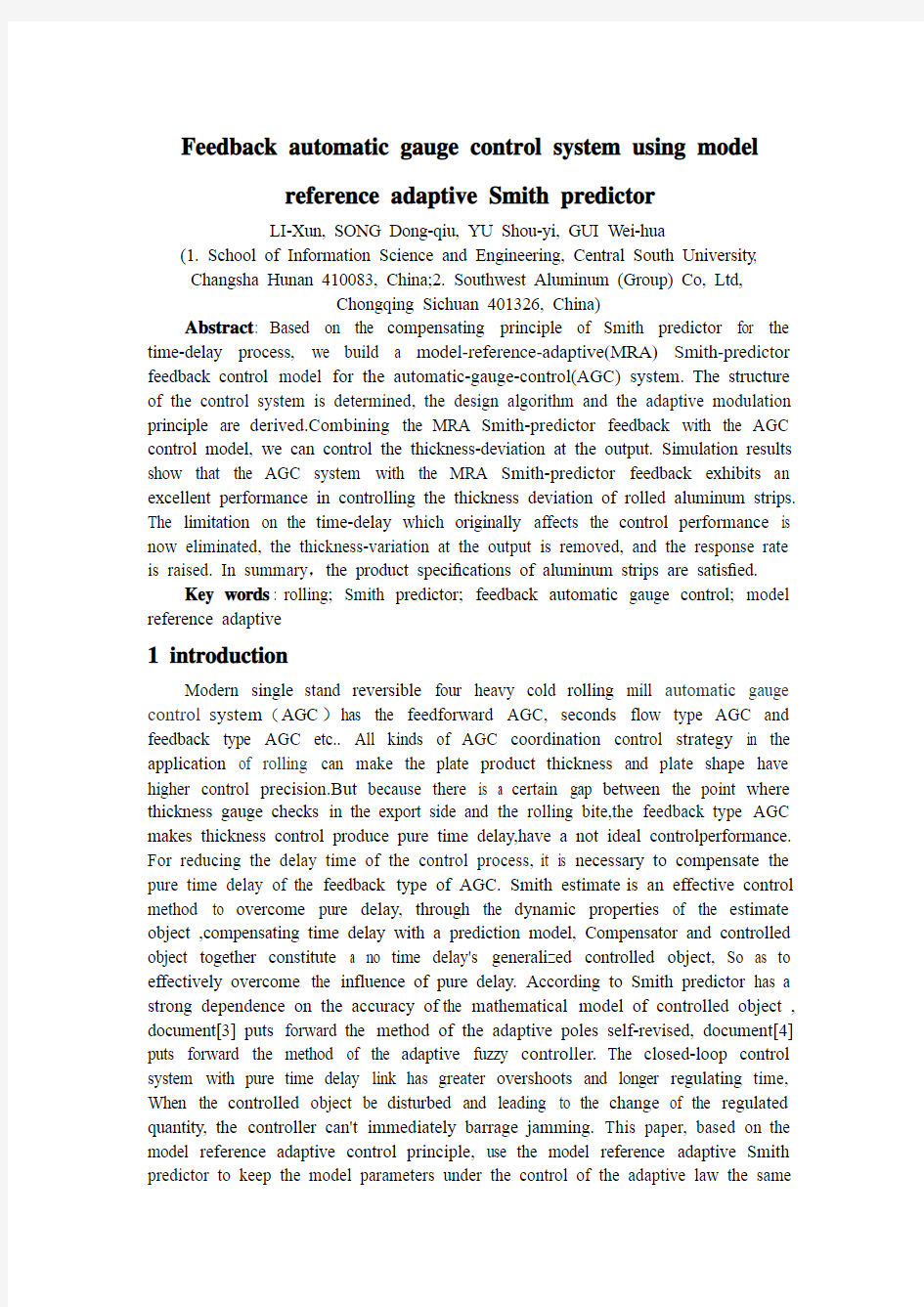
MRA-Smith predictor is presented in Figure 1. G(s)e-τs is the control system transfer function, G m(s)e-τms is Smith prediction model of the controlled object,
G C1(s) is the main controller,often use the PI algorithm. G C2(s) in the dotted line box is the secondary controller,often use the PD algorithm, Primarily for regulating the integral process or configurating the poles of the static process.Gd is the disturbance compensation controller.
GC2(s)used for stabilizing nonstatic integral process and configurating poles of dynamic process, makes the poles of the control system distribute in the right place,so there is a better control performance.Gd used to adjust the response characteristic of the disturbance d (t),inhibits the static error of standard Smith predictor with external disturbance,enhances adjust ability in order to improve the anti-jamming performance of the Smith predictor. For larger pure time delay object, Smith predictor with the PD secondary controller and disturbance compensation controller has a bettter control performance than the standard Smith predictor. In the cold rolling process rolling speed is change, Smith predictor model parameters and rolling mill parameters will not completely match, so join model reference adaptive agencies regulate the prediction model parameters,in order to reach the parameters which match the control object. G(e; t) is the gain of the adjustable feedforward regulator,F(e; t) is the compensation gain of the feedback regulator.When not joining MRA-Smith predictor, the closed-loop transfer function and characteristic equations of the control system is
Because of containing pure time delay link e-τs, along with the increase of τ and the phase lag, the stability of the system is lowering, the control effect become poor, the bigger τis the more difficult to stablize the system. When MRA-Smith predictor model and the controlled object is exactly match,C m(t) = C(t),G m(s) = G(s) and e-τms=e-τs.The output of system is
By formula (4), set characteristic equations of the input closed-loop transfer function as
Already not containing time delay part, the system stability does not influence byτ, e-τs in formula (4) only let the system response delay timeτ.
2.2Design of MRA-Smith predictor
Most of the controlled object of production process can be simplified by first-order lag plus delay(FOLPD),The transfer function is
In the formula,k is quotient,τ is the delay time,assume
Let the formula (8)(9)plug in formula (4),and ignore the time delay part e-τs,then get the input closed-loop transfer function
Assume
Simplify formula (10)as
according to the value of the given parameters kc,Ti,k and a,we can determine the value of the parameters η and c1, Ibrahim Kaya in the literature [10] put forward the relationship of d1 and c1 as following
2.3Design of MRA principle
Because the time delay part can be calculated,ignore the compensation pure time factor part of the rolling mill and Smith prediction model. According to formula (7),take the first order link of rolling mill as reference model,and the state equation is
Then the Smith predictor model adjustable system and its state equation is
The equation of Feedforward regulator G(e,t) and feedback regulator F(e,t) is
According to formula(15)(16),there is a adjustable system equation
Assume system general error as
According to formula (13)and(17),there is a generalized state error equation.
Therein
Design adaptive law of G (e,t) and F(e,t), make formula (19) asymptotically stable,when t→∞,e(t) →0, ψ(t) →0,φ(t)→0. Select the lyapunov function
In the function:λ1 > 0, λ2 > 0,km > 0,then v(t)>0 establishes when t≠0,so
Assume
Then
Ensure system is asymptotically stable,differentiate formula (20),and plug in formula (23) to get the system integral adaptive regulation law
3Feedback AGC system based on model reference adaptive Smith predictor
3.1 Feedback AGC system
According to the feedback type AGC system control principle, when there is incoming thickness deviation △H, rolled piece export thickness deviation is
In the formula: Q is the plastic stiffness of rolling piece, Cp is the longitudinal stiffness of rolling mill. To eliminate export thickness deviation, we need to adjust the amount of roll gap to
Set the distance thickness gauge to rolling mill roll gap as L,mill speed as v,the delay time to getting the detection value asτ1=L/v. Thickness gauge and down device has certain response time is respectively τm and τh,the total pure delay time of the feedback AGC control system is
3.2Exit-thickness deviation of MRA-Smith predictor feedback AGC
system
In feedback AGC control model reference adaptive Smith predictor can compensate the pure time delay factor e-τs. Figure 1 gets
According to formula(29),get the transfer function from Thickness deviation to roll gap
If Smith predictor model and rolling mill complete
match:G(s)e-τs=Gm(s)e-τms,plug (30) in (31) to get
Plug formula(33) and (34) in formula(32),then get the deviation value of the export thickness of rolled pieces
From formula (35) we can see the disturbance input is small, can even be neglected,the disturbance controller Gd takes zero,the deviation value of rolled piece export thickness is simplified to
Get △h to tend to 0,as long as configurating Gc2(s)=-1/Gm(s).
4Simulation of control system
4.1 Model structure of control system
In the feedback AGC control system, the thickness controller center on integrator, including thickness dead zone and the limiter. Because integrator generates oscillation and limit cycle oscillations easily, the goal of setting the dead zone is to prevent death
limit cycle oscillations, under the premise of ensuring the control accuracy to prevent hydraulic pressing device to produce false action. The limiter avoid the influence of the strip straightness of aluminum plate beacuse of the large amount of the roll gap regulating variable , ensure the precision of shape. MRA-Smith predictor is applied to the feedback AGC automatic thickness control, get the control system as shown in figure 2.
4.2Simulation parameters of control system
After simplified, single stand reversible four heavy cold rolling mill AGC system can be approach to 1-st order delay system, the mathematical model express as
Soτ/T=5.6,within the limits of 0.05≤τ/T≤6,according to the ITAE optimal PID controller design experience formula
Get the feedback AGC traditional PID controller
Rolling mill thickness gauge response time, feedback delay time and hydraulic pressure under device response time together is 0.3 s, set the sum of the input signal is the unit step signal. According to the above design principles, get MRA-Smith feedback AGC thickness control system parameters as shown in table 1.
4.3Simulation result of control system
According to the figure 2 build the SIMULINK simulation diagram of
MRA-Smith predictor of the feedback AGC control system,then get aluminum sheet exports thickness deviation curve as shown in fig.3.
Figure 3 (a) show that the traditional PID feedback AGC control system in aluminum sheet rolling process, because pure time delay characteristics is not compensated, aluminum sheet export thickness in about 3 s of the delay time do not reduce,thickness deviation curve is obviously oscillation. Conventional Smith feedback AGC control system can compensate for pure time delay characteristics of the rolling process, reduce oscillation of the exports thickness deviation curve, but there are a wave phenomenon, to a larger extent, slow reaction speed,after 2.5 s export thickness deviation reaches zero.
The predictor model and rolling mill model does not fit, assume the time constant of the Smith predictor model is 0.7 s (the actual time constant of rolling mill is 1 s) get export thickness deviation curve of rolled pieces as shown in figure 3 (b). MRA-Smith predictor feedback AGC thickness control system can start feed-forward regulator and feedback regulator according to the self-adaptive law,online
self-adaptive Smith predictor model parameters and rolling mill parameters tend to
match, make thickness deviation of rolled pieces gradually reach a set error range, not only compensate pure time delay characteristics existing in the feedback control, thickness deviation curve does not exist oscillation phenomena, the stability of system increases quickly, convergence time is in 0.5 s, self-adaptive response is fast , can satisfy the production accuracy of aluminum sheet.
5Conclusion
Feedback AGC thickness control system with pure time delay characteristics restrict the improvement of the quality of the board strips products, using the Smith predictor to compensate pure time delay is a kind of effective method in engineering. But the traditional Smith predictor is more sensitive in model parameter uncertainty,when the model not completely matching the performance of the control system is not good.The MRA-Smith is able to solve this problem, the key is to build compensator model and realize pure delay link and design self-adaptive law. In this paper, we study the MRA-Smith prediction PI controller feedback AGC control
system’s application in aluminum sheet rolling process AGC control, AGC the results show that the Smith predictor with improved structure combined with the adaptive regulation law can solve the problem that the phenomena model parameters are not completely matching influences control performance,let rolled piece export thickness deviation be quickly in the allowable range in the fast time,the control response be fast, and effectively compensate for pure time delay characteristics of the traditional PI thickness control , rolled pieces thickness control have high accuracy, and there is engineering application value.
M A T L A B模型预测控制工具箱函数 8.2系统模型建立与转换函数 前面读者论坛了利用系统输入/输出数据进行系统模型辨识的有关函数及使用方法,为时行模型预测控制器的设计,需要对系统模型进行进一步的处理和转换。MATLAB的模型预测控制工具箱中提供了一系列函数完成多种模型转换和复杂系统模型的建立功能。 在模型预测控制工具箱中使用了两种专用的系统模型格式,即MPC状态空间模型和MPC传递函数模型。这两种模型格式分别是状态空间模型和传递函数模型在模型预测控制工具箱中的特殊表达形式。这种模型格式化可以同时支持连续和离散系统模型的表达,在MPC传递函数模型中还增加了对纯时延的支持。表8-2列出了模型预测控制工具箱的模型建立与转换函数。 表8-2模型建立与转换函数 8.2.1模型转换 在MATLAB模型预测工具箱中支持多种系统模型格式。这些模型格式包括: ①通用状态空间模型; ②通用传递函数模型; ③MPC阶跃响应模型; ④MPC状态空间模型;
⑤MPC传递函数模型。 在上述5种模型格式中,前两种模型格式是MATLAB通用的模型格式,在其他控制类工具箱中,如控制系统工具箱、鲁棒控制工具等都予以支持;而后三种模型格式化则是模型预测控制工具箱特有的。其中,MPC状态空间模型和MPC传递函数模型是通用的状态空间模型和传递函数模型在模型预测控制工具箱中采用的增广格式。模型预测控制工具箱提供了若干函数,用于完成上述模型格式间的转换功能。下面对这些函数的用法加以介绍。 1.通用状态空间模型与MPC状态空间模型之间的转换 MPC状态空间模型在通用状态空间模型的基础上增加了对系统输入/输出扰动 和采样周期的描述信息,函数ss2mod()和mod2ss()用于实现这两种模型格式之间的转换。 1)通用状态空间模型转换为MPC状态空间模型函数ss2mod() 该函数的调用格式为 pmod=ss2mod(A,B,C,D) pmod=ss2mod(A,B,C,D,minfo) pmod=ss2mod(A,B,C,D,minfo,x0,u0,y0,f0) 式中,A,B,C,D为通用状态空间矩阵; minfo为构成MPC状态空间模型的其他描述信息,为7个元素的向量,各元素分别定义为: ◆minfo(1)=dt,系统采样周期,默认值为1; ◆minfo(2)=n,系统阶次,默认值为系统矩阵A的阶次; ◆minfo(3)=nu,受控输入的个数,默认值为系统输入的维数; ◆minfo(4)=nd,测量扰的数目,默认值为0; ◆minfo(5)=nw,未测量扰动的数目,默认值为0; ◆minfo(6)=nym,测量输出的数目,默认值系统输出的维数; ◆minfo(7)=nyu,未测量输出的数目,默认值为0; 注:如果在输入参数中没有指定m i n f o,则取默认值。 x0,u0,y0,f0为线性化条件,默认值均为0; pmod为系统的MPC状态空间模型格式。 例8-5将如下以传递函数表示的系统模型转换为MPC状态空间模型。 解:MATLAB命令如下:
云南大学信息学院学生实验报告 课程名称:现代控制理论 实验题目:预测控制 小组成员:李博(12018000748) 金蒋彪(12018000747) 专业:2018级检测技术与自动化专业
1、实验目的 (3) 2、实验原理 (3) 2.1、预测控制特点 (3) 2.2、预测控制模型 (4) 2.3、在线滚动优化 (5) 2.4、反馈校正 (5) 2.5、预测控制分类 (6) 2.6、动态矩阵控制 (7) 3、MATLAB仿真实现 (9) 3.1、对比预测控制与PID控制效果 (9) 3.2、P的变化对控制效果的影响 (12) 3.3、M的变化对控制效果的影响 (13) 3.4、模型失配与未失配时的控制效果对比 (14) 4、总结 (15) 5、附录 (16) 5.1、预测控制与PID控制对比仿真代码 (16) 5.1.1、预测控制代码 (16) 5.1.2、PID控制代码 (17) 5.2、不同P值对比控制效果代码 (19) 5.3、不同M值对比控制效果代码 (20) 5.4、模型失配与未失配对比代码 (20)
1、实验目的 (1)、通过对预测控制原理的学习,掌握预测控制的知识点。 (2)、通过对动态矩阵控制(DMC)的MATLAB仿真,发现其对直接处理具有纯滞后、大惯性的对象,有良好的跟踪性和较强的鲁棒性,输入已 知的控制模型,通过对参数的选择,来获得较好的控制效果。 (3)、了解matlab编程。 2、实验原理 模型预测控制(Model Predictive Control,MPC)是20世纪70年代提出的一种计算机控制算法,最早应用于工业过程控制领域。预测控制的优点是对数学模型要求不高,能直接处理具有纯滞后的过程,具有良好的跟踪性能和较强的抗干扰能力,对模型误差具有较强的鲁棒性。因此,预测控制目前已在多个行业得以应用,如炼油、石化、造纸、冶金、汽车制造、航空和食品加工等,尤其是在复杂工业过程中得到了广泛的应用。在分类上,模型预测控制(MPC)属于先进过程控制,其基本出发点与传统PID控制不同。传统PID控制,是根据过程当前的和过去的输出测量值与设定值之间的偏差来确定当前的控制输入,以达到所要求的性能指标。而预测控制不但利用当前时刻的和过去时刻的偏差值,而且还利用预测模型来预估过程未来的偏差值,以滚动优化确定当前的最优输入策略。因此,从基本思想看,预测控制优于PID控制。 2.1、预测控制特点 首先,对于复杂的工业对象。由于辨识其最小化模型要花费很大的代价,往往给基于传递函数或状态方程的控制算法带来困难,多变量高维度复杂系统难以建立精确的数学模型工业过程的结构、参数以及环境具有不确定性、时变性、非线性、强耦合,最优控制难以实现。而预测控制所需要的模型只强调其预测功能,不苛求其结构形式,从而为系统建模带来了方便。在许多场合下,只需测定对象的阶跃或脉冲响应,便可直接得到预测模型,而不必进一步导出其传递函数或状
神经网络模型预测控制器 摘要:本文将神经网络控制器应用于受限非线性系统的优化模型预测控制中,控制规则用一个神经网络函数逼近器来表示,该网络是通过最小化一个与控制相关的代价函数来训练的。本文提出的方法可以用于构造任意结构的控制器,如减速优化控制器和分散控制器。 关键字:模型预测控制、神经网络、非线性控制 1.介绍 由于非线性控制问题的复杂性,通常用逼近方法来获得近似解。在本文中,提出了一种广泛应用的方法即模型预测控制(MPC),这可用于解决在线优化问题,另一种方法是函数逼近器,如人工神经网络,这可用于离线的优化控制规则。 在模型预测控制中,控制信号取决于在每个采样时刻时的想要在线最小化的代价函数,它已经广泛地应用于受限的多变量系统和非线性过程等工业控制中[3,11,22]。MPC方法一个潜在的弱点是优化问题必须能严格地按要求推算,尤其是在非线性系统中。模型预测控制已经广泛地应用于线性MPC问题中[5],但为了减小在线计算时的计算量,该部分的计算为离线。一个非常强大的函数逼近器为神经网络,它能很好地用于表示非线性模型或控制器,如文献[4,13,14]。基于模型跟踪控制的方法已经普遍地应用在神经网络控制,这种方法的一个局限性是它不适合于不稳定地逆系统,基此本文研究了基于优化控制技术的方法。 许多基于神经网络的方法已经提出了应用在优化控制问题方面,该优化控制的目标是最小化一个与控制相关的代价函数。一个方法是用一个神经网络来逼近与优化控制问题相关联的动态程式方程的解[6]。一个更直接地方法是模仿MPC方法,用通过最小化预测代价函数来训练神经网络控制器。为了达到精确的MPC技术,用神经网络来逼近模型预测控制策略,且通过离线计算[1,7.9,19]。用一个交替且更直接的方法即直接最小化代价函数训练网络控制器代替通过训练一个神经网络来逼近一个优化模型预测控制策略。这种方法目前已有许多版本,Parisini[20]和Zoppoli[24]等人研究了随机优化控制问题,其中控制器作为神经网络逼近器的输入输出的一个函数。Seong和Widrow[23]研究了一个初始状态为随机分配的优化控制问题,控制器为反馈状态,用一个神经网络来表示。在以上的研究中,应用了一个随机逼近器算法来训练网络。Al-dajani[2]和Nayeri等人[15]提出了一种相似的方法,即用最速下降法来训练神经网络控制器。 在许多应用中,设计一个控制器都涉及到一个特殊的结构。对于复杂的系统如减速控制器或分散控制系统,都需要许多输入与输出。在模型预测控制中,模型是用于预测系统未来的运动轨迹,优化控制信号是系统模型的系统的函数。因此,模型预测控制不能用于定结构控制问题。不同的是,基于神经网络函数逼近器的控制器可以应用于优化定结构控制问题。 在本文中,主要研究的是应用于非线性优化控制问题的结构受限的MPC类型[20,2,24,23,15]。控制规则用神经网络逼近器表示,最小化一个与控制相关的代价函数来离线训练神经网络。通过将神经网络控制的输入适当特殊化来完成优化低阶控制器的设计,分散和其它定结构神经网络控制器是通过对网络结构加入合适的限制构成的。通过一个数据例子来评价神经网络控制器的性能并与优化模型预测控制器进行比较。 2.问题表述 考虑一个离散非线性控制系统: 其中为控制器的输出,为输入,为状态矢量。控制
M A T L A B模型预测控制 工具箱函数 TTA standardization office【TTA 5AB- TTAK 08- TTA 2C】
M A T L A B模型预测控制工具箱函数 系统模型建立与转换函数 前面读者论坛了利用系统输入/输出数据进行系统模型辨识的有关函数及使用方法,为时行模型预测控制器的设计,需要对系统模型进行进一步的处理和转换。MATLAB的模型预测控制工具箱中提供了一系列函数完成多种模型转换和复杂系统模型的建立功能。 在模型预测控制工具箱中使用了两种专用的系统模型格式,即MPC状态空间模型和MPC传递函数模型。这两种模型格式分别是状态空间模型和传递函数模型在模型预测控制工具箱中的特殊表达形式。这种模型格式化可以同时支持连续和离散系统模型的表达,在MPC传递函数模型中还增加了对纯时延的支持。表8-2列出了模型预测控制工具箱的模型建立与转换函数。 表8-2 模型建立与转换函数 模型转换 在MATLAB模型预测工具箱中支持多种系统模型格式。这些模型格式包括: ①通用状态空间模型; ②通用传递函数模型; ③MPC阶跃响应模型; ④MPC状态空间模型; ⑤MPC传递函数模型。
在上述5种模型格式中,前两种模型格式是MATLAB通用的模型格式,在其他控制类工具箱中,如控制系统工具箱、鲁棒控制工具等都予以支持;而后三种模型格式化则是模型预测控制工具箱特有的。其中,MPC状态空间模型和MPC传递函数模型是通用的状态空间模型和传递函数模型在模型预测控制工具箱中采用的增广格式。模型预测控制工具箱提供了若干函数,用于完成上述模型格式间的转换功能。下面对这些函数的用法加以介绍。 1.通用状态空间模型与MPC状态空间模型之间的转换 MPC状态空间模型在通用状态空间模型的基础上增加了对系统输入/输出扰动和采样周期的描述信息,函数ss2mod()和mod2ss()用于实现这两种模型格式之间的转换。 1)通用状态空间模型转换为MPC状态空间模型函数ss2mod() 该函数的调用格式为 pmod= ss2mod(A,B,C,D) pmod= ss2mod(A,B,C,D,minfo) pmod= ss2mod(A,B,C,D,minfo,x0,u0,y0,f0) 式中,A, B, C, D为通用状态空间矩阵; minfo为构成MPC状态空间模型的其他描述信息,为7个元素的向量,各元素分别定义为: ◆minfo(1)=dt,系统采样周期,默认值为1; ◆minfo(2)=n,系统阶次,默认值为系统矩阵A的阶次; ◆minfo(3)=nu,受控输入的个数,默认值为系统输入的维数; ◆minfo(4)=nd,测量扰的数目,默认值为0; ◆minfo(5)=nw,未测量扰动的数目,默认值为0; ◆minfo(6)=nym,测量输出的数目,默认值系统输出的维数; ◆minfo(7)=nyu,未测量输出的数目,默认值为0; 注:如果在输入参数中没有指定m i n f o,则取默认值。 x0, u0, y0, f0为线性化条件,默认值均为0; pmod为系统的MPC状态空间模型格式。 例8-5将如下以传递函数表示的系统模型转换为MPC状态空间模型。 解:MATLAB命令如下:
模型预测控制快速求解算法 模型预测控制(Model Predictive Control,MPC)是一种基于在线计算的控制优化算法,能够统一处理带约束的多参数优化控制问题。当被控对象结构和环境相对复杂时,模型预测控制需选择较大的预测时域和控制时域,因此大大增加了在线求解的计算时间,同时降低了控制效果。从现有的算法来看,模型预测控制通常只适用于采样时间较大、动态过程变化较慢的系统中。因此,研究快速模型预测控制算法具有一定的理论意义和应用价值。 虽然MPC方法为适应当今复杂的工业环境已经发展出各种智能预测控制方法,在工业领域中也得到了一定应用,但是算法的理论分析和实际应用之间仍然存在着一定差距,尤其在多输入多输出系统、非线性特性及参数时变的系统和结果不确定的系统中。预测控制方法发展至今,仍然存在一些问题,具体如下: ①模型难以建立。模型是预测控制方法的基础,因此建立的模型越精确,预测控制效果越好。尽管模型辨识技术已经在预测控制方法的建模过程中得以应用,但是仍无法建立非常精确的系统模型。 ②在线计算过程不够优化。预测控制方法的一大特征是在线优化,即根据系统当前状态、性能指标和约束条件进行在线计算得到当前状态的控制律。在在线优化过程中,当前的优化算法主要有线性规划、二次规划和非线性规划等。在线性系统中,预测控制的在线计算过程大多数采用二次规划方法进行求解,但若被控对象的输入输出个数较多或预测时域较大时,该优化方法的在线计算效率也会无法满足系统快速性需求。而在非线性系统中,在线优化过程通常采用序列二次优化算法,但该方法的在线计算成本相对较高且不能完全保证系统稳定,因此也需要不断改进。 ③误差问题。由于系统建模往往不够精确,且被控系统中往往存在各种干扰,预测控制方法的预测值和实际值之间一定会产生误差。虽然建模误差可以通过补偿进行校正,干扰误差可以通过反馈进行校正,但是当系统更复杂时,上述两种校正结合起来也无法将误差控制在一定范围内。 模型预测控制区别于其它算法的最大特征是处理多变量多约束线性系统的能力,但随着被控对象的输入输出个数的增多,预测控制方法为保证控制输出的精确性,往往会选取较大的预测步长和控制步长,但这样会大大增加在线优化过程的计算量,从而需要更多的计算时间。因此,预测控制方法只能适用于采样周
MATLAB模型预测控制工具箱函数 8.2 系统模型建立与转换函数 前面读者论坛了利用系统输入/输出数据进行系统模型辨识的有关函数及使用方法,为时行模型预测控制器的设计,需要对系统模型进行进一步的处理和转换。MATLAB的模型预测控制工具箱中提供了一系列函数完成多种模型转换和复杂系统模型的建立功能。 在模型预测控制工具箱中使用了两种专用的系统模型格式,即MPC状态空间模型和MPC传递函数模型。这两种模型格式分别是状态空间模型和传递函数模型在模型预测控制工具箱中的特殊表达形式。这种模型格式化可以同时支持连续和离散系统模型的表达,在MPC传递函数模型中还增加了对纯时延的支持。表8-2列出了模型预测控制工具箱的模型建立与转换函数。 表8-2 模型建立与转换函数 8.2.1 模型转换 在MATLAB模型预测工具箱中支持多种系统模型格式。这些模型格式包括: ①通用状态空间模型; ②通用传递函数模型; ③MPC阶跃响应模型; ④MPC状态空间模型;
⑤ MPC 传递函数模型。 在上述5种模型格式中,前两种模型格式是MATLAB 通用的模型格式,在其他控制类工具箱中,如控制系统工具箱、鲁棒控制工具等都予以支持;而后三种模型格式化则是模型预测控制工具箱特有的。其中,MPC 状态空间模型和MPC 传递函数模型是通用的状态空间模型和传递函数模型在模型预测控制工具箱中采用的增广格式。模型预测控制工具箱提供了若干函数,用于完成上述模型格式间的转换功能。下面对这些函数的用法加以介绍。 1.通用状态空间模型与MPC 状态空间模型之间的转换 MPC 状态空间模型在通用状态空间模型的基础上增加了对系统输入/输出扰动和采样周期的描述信息,函数ss2mod ()和mod2ss ()用于实现这两种模型格式之间的转换。 1)通用状态空间模型转换为MPC 状态空间模型函数ss2mod () 该函数的调用格式为 pmod= ss2mod (A,B,C,D) pmod = ss2mod (A,B,C,D,minfo) pmod = ss2mod (A,B,C,D,minfo,x0,u0,y0,f0) 式中,A, B, C, D 为通用状态空间矩阵; minfo 为构成MPC 状态空间模型的其他描述信息,为7个元素的向量,各元素分别定义为: ◆ minfo(1)=dt ,系统采样周期,默认值为1; ◆ minfo(2)=n ,系统阶次,默认值为系统矩阵A 的阶次; ◆ minfo(3)=nu ,受控输入的个数,默认值为系统输入的维数; ◆ minfo(4)=nd ,测量扰的数目,默认值为0; ◆ minfo(5)=nw ,未测量扰动的数目,默认值为0; ◆ minfo(6)=nym ,测量输出的数目,默认值系统输出的维数; ◆ minfo(7)=nyu ,未测量输出的数目,默认值为0; 注:如果在输入参数中没有指定m i n f o ,则取默认值。 x0, u0, y0, f0为线性化条件,默认值均为0; pmod 为系统的MPC 状态空间模型格式。 例8-5 将如下以传递函数表示的系统模型转换为MPC 状态空间模型。 1 2213)(232+++++=s s s s s s G 解:MATLAB 命令如下:
11.预测控制与预见控制 11.1概述 在我们的日常生活,根据未来的情况而决定现在的行动的事例比比皆是。如,估计天气会下雨,出门时带上伞;看到前面路上有凹凸不平,提前把车速减下来,等等。有必要提起注意的是,这里举出的两例对“未来情况”的把握是存在差异的,前者只是一种“估计”或者说“预测”(是否下雨并不一定),而后者却是明明白白看到了一个事实(确实有凹凸),我们权且称为“预见”。在控制工程中,依据对未来情况的“预测“或“预见”来决定当前控制输入的控制方法便是我们要讨论的“预测控制”(Prdeictive Control)和“预见控制”(Preview Control)。 所谓预测控制,是指根据某种方法对系统未来的输出进行预测,并导求一种使预测的输出与期望值之间的误差尽可能小的控制方法,比较有代表性的有模型算法控制(MAC----Model Algorifhmic Control)、动态矩阵控制(DMC----Dynamic Matrix Control)等,这些方法直接从系统的预测模型(非参数模型),并根据某一优化指标设计控制系统,确定一个控制量的时间序列,使未来一段时间内输出量与期望量之间的误差最小。由于这种控制方法的数模通过简单的实验得到,无须深入了解系统或过程的内部结构,也不必进行复杂的系统辩识,建模容易、简单,而且在算法中采用滚动优化策略,并在优化过程中不断通过实测系统输出与预测模型输出的误差来进行反馈校正,能在一定程度上克服由于预测模型误差和某些不确定干扰等的影响,所以特别适用于复杂工业生产过程的控制,在化工、冶金、石油、电力等部门得到了成功应用。80年代初,人们结合自适应控制的研究,又发展了一些基于辩识过程参数模型,如广义预测控制(GPC Generalized Predictive Control)等。 与预测控制不同的是,预见控制对未来情报的了解和掌握不是基于某种推测或判断,预见控制是基于一个控制对象的模型是已知的,系统中未来的目标值或外扰是可以通过某种手段预先明确地得知和确定的假设,也就是说,预见控制是根据已经确认的系统未来应该满足什么要求,系统未来的目标信号或外部干扰将会有怎样的变化等信息来做出当前时刻的控制决策。预见控制中有时以最优控制理论(optimal Control theory)作为理论基础和求解手段,但它追求的不仅是