On Parallel Implementations of Dynamic
Overset Grid Methods
Andrew M. Wissink
Research Scientist, MCAT Inc.
Robert L. Meakin
Research Scientist, U.S. Army Aero?ightdynamics Directorate, AMCOM
NASA Ames Research Center, Mailstop 258-1
Moffett Field, CA 94035-1000
[wissink,meakin]@https://www.doczj.com/doc/0915424133.html,
Abstract
This paper explores the parallel performance of structured overset CFD computations for multi-component bodies in which there is relative motion between component parts. The two processes that dominate the cost of such problems are the ?ow solution on each component and the inter-grid connectivity solution. A two-part static-dynamic load balancing scheme is proposed in which the static part balances the load for the ?ow solution and the dynamic part re-balances, if necessary, the load for the connectivity solution. This scheme is coupled with existing parallel implementations of the OVERFLOW ?ow solver and DCF3D connectivity routine and used for unsteady calculations about aerodynamic bodies on the IBM SP2 and IBM SP multi-processors. This paper also describes the parallel implementation of a new solution-adaption scheme based on structured Cartesian overset grids.
1.0 Introduction
Unsteady prediction of viscous ?ows with relative movement between component parts remains an extremely challenging problem facing Computational Fluid Dynamics (CFD) researchers today. While unstructured-grid methods have shown impressive results for inviscid moving-grid simulations [1], dynamic overset structured-grid schemes based on the “Chimera”
[2] approach have demonstrated the most success for viscous moving-grid problems that experi-ence arbitrary motion. There are a number of dif?cult problems for which dynamic overset grid schemes have been exclusively applied, including space shuttle booster separation [3], missile store separation [4], and helicopters with moving rotor blades [5]. Navier-Stokes calculations with these methods require high computational resources that overwhelm vector-based machines like the Cray C90. Large multi-processor such as the IBM SP and Cray T3E offer the potential for dramatic increases in available computing power but scalable implementations of existing applications software must be devised if the power of these machines is to be fully realized.
A number of researchers have investigated the parallel performance of overlapping grid schemes for steady-state CFD calculations [6-8] but only the works of Weeratunga and Barszcz [9,10] directly address their parallel performance when applied to moving-grid problems. In addition to the ?ow calculation, moving-grid applications require that interpolation coef?cients
between the various overlapping grid components be updated at each timestep. The connectivity solution can constitute a signi?cant fraction (10-50%) of the total computational work and can be dif?cult to parallelize ef?ciently. A partitioning strategy that gives optimal parallel performance in the ?ow solution does not necessarily give optimal performance in the connectivity solution, and vice-versa. Therefore, alternative parallel implementation approaches must be considered to attain scalable performance on large numbers of processors for moving-grid problems.
Although Weeratunga and Barszcz introduced novel parallel implementations of both the ?ow and connectivity solutions, they did not directly address optimal load balancing techniques for parallel ef?ciency of the connectivity solution.This paper seeks to extend their work by propos-ing a load balancing approach to improve the parallel ef?ciency for moving-grid applications. The paper is divided into six sections. The second section gives details about the parallel imple-mentations for the ?ow solver and connectivity routine. The third section introduces a static and a dynamic load balancing approach. Section four presents results of the parallel performance on the IBM SP2 and IBM SP for unsteady Navier-Stokes calculations about three different aerody-namic con?gurations. Section ?ve discusses a new approach for overset grid problems which will be followed in future work. Finally, some concluding remarks are given in section six.
2.0 Dynamic Overset Grid Scheme
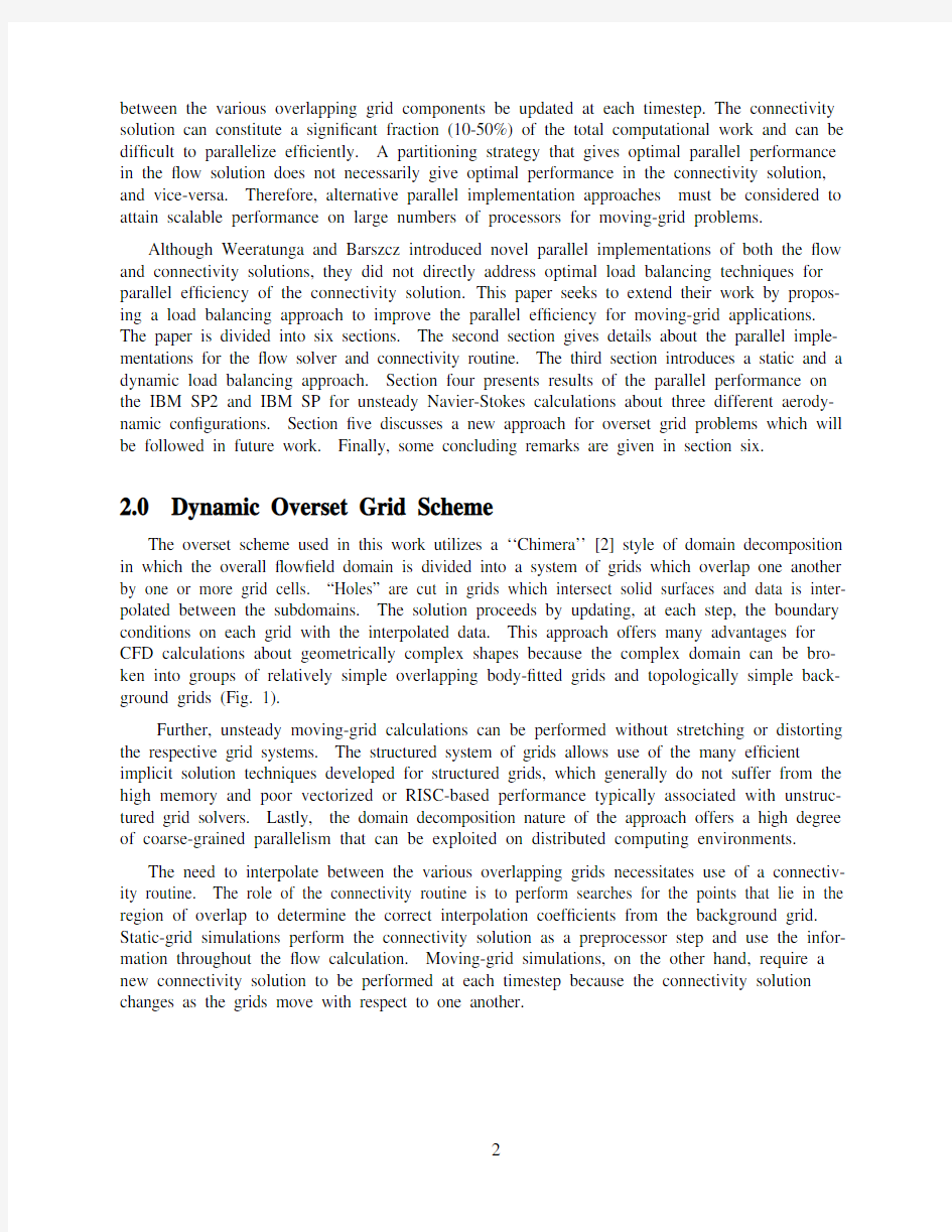
The overset scheme used in this work utilizes a ‘‘Chimera’’ [2] style of domain decomposition in which the overall ?ow?eld domain is divided into a system of grids which overlap one another by one or more grid cells. “Holes” are cut in grids which intersect solid surfaces and data is inter-polated between the subdomains. The solution proceeds by updating, at each step, the boundary conditions on each grid with the interpolated data. This approach offers many advantages for CFD calculations about geometrically complex shapes because the complex domain can be bro-ken into groups of relatively simple overlapping body-?tted grids and topologically simple back-ground grids (Fig. 1).
Further, unsteady moving-grid calculations can be performed without stretching or distorting the respective grid systems. The structured system of grids allows use of the many ef?cient implicit solution techniques developed for structured grids, which generally do not suffer from the high memory and poor vectorized or RISC-based performance typically associated with unstruc-tured grid solvers. Lastly, the domain decomposition nature of the approach offers a high degree of coarse-grained parallelism that can be exploited on distributed computing environments.
The need to interpolate between the various overlapping grids necessitates use of a connectiv-ity routine. The role of the connectivity routine is to perform searches for the points that lie in the region of overlap to determine the correct interpolation coef?cients from the background grid. Static-grid simulations perform the connectivity solution as a preprocessor step and use the infor-mation throughout the ?ow calculation. Moving-grid simulations, on the other hand, require a new connectivity solution to be performed at each timestep because the connectivity solution changes as the grids move with respect to one another.
Figure 1. Overset grid system for V-22 tiltrotor
Three main pieces of software are used in the parallel dynamic overset scheme explored in this work. The ?ow solution on overlapping grid components is performed using NASA’s struc-tured-grid ?ow solver OVERFLOW by Buning [11]. Grid motion is determined by a six degree of freedom model (SIXDOF) [4], and connectivity between the overlapping grids at each timestep is performed using the code DCF3D of Meakin [12]. The parallel implementations of OVERFLOW and DCF3D previously introduced by Weeratunga [9] and Barszcz [10], respectively, are used. The load balancing scheme proposed here is incorporated and the entire package is bundled into a single code called OVERFLOW-D1.
An unsteady ?ow calculation using OVERFLOW-D1 involves three main steps carried out at each timestep: 1) solve the nonlinear ?uid ?ow equations (Euler/Navier-Stokes) subject to ?ow and intergrid boundary conditions, 2) move grid components associated with moving bodies sub-ject to applied and aerodynamic loads (or according to a prescribed path), 3) re-establish domain connectivity for the system of overlapping grids. Each step of the solution proceeds separately and barriers are put in place to synchronize each of the solution modules.
2.1 OVERFLOW Parallel Implementation
The parallel implementation approach of OVERFLOW uses both coarse-grained parallelism between grids and ?ne-grained parallelism within grids. Processor groups are assigned to each grid component and each processor executes its own version of the code for the grid or portion of the grid assigned to it (Fig. 2). The spatial accuracy is second order and temporal accuracy is ?rst order. The solution is marched in time using a diagonalized approximate factorization scheme. Implicitness is maintained across the subdomains on each component so the solution convergence characteristics remain unchanged with different numbers of processors. More details about the ?ow solver and parallel implementation are available in Refs. [8,9]. The approach is designed for
execution on a Multiple Instruction Multiple Data (MIMD) distributed-memory parallel com-puter. Communication between the processor subdomains is performed with MPI [13] subroutine calls.
2.2 DCF3D Parallel Implementation
The parallel approach for the donor search routine in DCF3D was originally devised by Barszcz [10]. The user provides input for each grid and a list of component grids that should be searched to ?nd donor points for each of the inter-grid boundary points (IGBPs) on the processor.The grids are listed in hierarchical manner with the corresponding grids searched in the order they are listed. The donor search procedure performed with in DCF3D proceeds as follows at each timestep:
?Each processor consults the search list to determine the component grid from which to request a search. It then checks the bounding boxes of each of the processors assigned to that grid. This can be determined locally since the bounding box information is
broadcast globally at the beginning of the solution.
?Based on the bounding-box information, the processor determines which processor to send its search request to. A list of inter-grid boundary points (IGBPs) is sent to that
processor which performs the search for the donor locations on its grid.
?Once all locations have been searched, the information is sent back to the calling proces-sor and the IGBPs which have donors (i.e. those for which the search was successful) are
tagged.
Figure 2. Grid-based parallel implementation approach for OVERFLOW
2D Oscillating Airfoil
3 Grids/9 processors
If all IGBPs have not received a donor, the procedure is repeated for the next grid in the hierarchy.If the search happens to hit a processor boundary, the search request is forwarded to the neighbor-ing processor on the grid and the search is continued. This process is illustrated in Fig. 3.
The messages requesting searches are all sent asynchronously so that processors can be per-forming searches simultaneously. For example, after processor 1 sends a list of its IGBPs for a non-local search to processor 2, it checks if any other processors have requested searches of it. If any have, processor 1 performs the search and returns the result to the calling processor before checking if processor 2 has returned the results of its search request.
The most computationally intensive part of the connectivity solution algorithm above is per-forming the donor search requests (step 3). There is nearly always a load imbalance in this step because certain processors hold data where many searches take place while others hold data where few searches are required.
In performing the connectivity solution at the ?rst timestep, nothing is known about the possi-ble donor location and the solution must be performed from scratch. In subsequent timesteps,however, the known donor locations from the previous timestep can be used as a starting point for the searches at the new timestep. This idea, referred to as “nth-level-restart”, was proposed by Barszcz [10] and was found to yield a considerable reduction in the time spent in the connectivity solution. The maximum timestep used in the problem is most often governed by stability condi-tions of the ?ow solver and this timestep is generally small enough that the donor cell locations do not move by more than one cell of the receiving grid per timestep. It is for this reason that the nth-level-restart idea tends to be quite effective at reducing the search costs.
3.0 Load Balance
Poor load balance is the primary source of parallel inef?ciency using the parallel moving-body overset scheme. The two dominant computational costs in the calculation are the ?ow solu-1
234Send List Perform
Search
Send back donor locations
Form IGBP list Processor 1
Processor 2
Figure 3. DCF3D parallel implementation approach - distributed donor search procedure
tion and domain connectivity solution and the ef?ciency is best if both are load balanced. Unfor-tunately, devising a scheme that can effectively load balance both the ?ow solution and connectivity solution is dif?cult.
The load balance of the ?ow solution is proportional to the volume of gridpoints on each pro-cessor. While some variation arises from differences in the computational work per gridpoint (e.g. some grids may be viscous while others are inviscid, turbulence model may be employed on some grids but not others, etc.), the differences are not substantial for the cases presented in this work.
A static load balancing scheme is applied initially which seeks to distribute the volume of gridpoints in the subdomains as evenly as possible. The routine takes as input the number of grids, their indices, and the total number of processors to be applied to the problem and deter-mines the number of processors that should be applied to each grid to distribute the gridpoints as evenly as possible. The algorithm used to achieve this result is as follows:
Algorithm 1: Static Load Balance Routine
g(n) = number of gridpoints in component grid n
G = total number of gridpoints from all grids np(n) = number of processors applied to component n
NP = total number of processors
, = tolerance factor, increment
1.Initialize : Compute g(n),G ; set and ; set to small value (~0.1)
2.DO until ?, with condition that ??END DO
In Algorithm 1,ε is initially the most ef?cient load balance possible, equal to the total number of gridpoints over the total number of processors. Then, the number of subdomains np(n) is com-puted for grid n by dividing the number of gridpoints g(n) by ε. The g(n) value is inclusive of the points which are eventually blanked out in the connectivity solution. Unless the grids are per-fectly divisible by ε, the resulting total number of subdomains is less than the number of proces-sors. Thus, a tolerance factor τ is incremented by ?τ and the process is repeated until the number of subdomains equals the number of processors. If τ=0, the problem is perfectly load balanced.Increasingly greater values of τ indicates higher degrees of load imbalance. Thus, the tolerance factor is a measure of the degree of load imbalance.
Because Algorithm 1 uses integer arithmetic, there arises the possibility of having in?nite solutions with certain grid and processor partition choices, for which the algorithm will not con-verge. For example, if three processors are applied to two equally-sized grids (i.e. same g(n)), the algorithm cannot decide which grid should receive two processors and which should receive one
G g n ()
∑=τ?τεG NP
-------=τ0=?τnp n ()∑NP
=np n ()int g n ()ε
----------=np n ()1≥ττ?τ
+=εε1τ+()
?=
and will continue iterating. A special condition has been put in place for these cases; If the
method proceeds for many iterations and does not converge, the value of the grid index n is added to g(n) and the method is repeated. Since n is generally very small relative to g(n),this effectively adds a small perturbation to the system and the method will subsequently converge.
Once the number of processors applied to each grid is determined, the routine divides the grids into subdomains with the smallest surface area based on the index space of the grid. The routine forms subdomains based on the prime factors of np(n). For example, if np(n)=12, the prime factors are 3, 2, and 2. It divides the largest dimension in the domain by 3, then subdivides the largest dimension in each subdomain by 2, and further subdivides the largest dimension in each sub-subdomain by 2. In this way, the algorithm forms subdomains which have index spaces that are as close to cubic as possible, thereby minimizing the surface area in order to minimize communication between the subdomains (Fig. 4).
The static load balancing scheme is effective at load balancing the ?ow solution but makes no effort to load balance the connectivity solution. In some cases, namely those which have a large number of inter-grid boundary points relative to the number of gridpoints, the connectivity solu-tion can represent a signi?cant proportion of the computational cost. It is therefore desirable to have in place a means of load balancing the connectivity solution for use with these cases.The primary computational costs in the connectivity solution are incurred in facilitating the donor search requests sent by other processors (step 3 in Fig. 3). The donor search costs are pro-portional to the number of non-local IGBPs, located on other processors, sent to the local proces-sor in the search request. Thus, an ef?cient load balancing strategy for the connectivity solution
should seek to equally distribute the number of non-local IGBPs sent to each processor.
Index Space of Grids Grids Divided into Subdomains
Figure 4. Static load balance routine
A dynamic scheme is proposed for load balancing the connectivity solution. The necessity of a dynamic scheme is twofold. First, determining a prediction locally of the number of IGBPs that will be sent by other processors is dif?cult to do apriori because it requires all non-local data. It is generally easier to begin the calculation and determine the degree of imbalance after a few steps of the solution than it is to predict the imbalance before the start of the solution. Second, the num-ber of search requests will change throughout a moving-grid calculation as grids pass through each other so a dynamic scheme will adapt the load balance as the problem changes. The pro-posed dynamic scheme is given in Algorithm 2.
Algorithm 2: Dynamic Load Balance Scheme
f o = user speci?ed load balance factor
1. Begin solution - apply static load balance routine
2. Check solution after speci?ed number of timesteps:
?Determine I(p) = #IGBPs received on processor p
?Compute (global average over all processors)?Compute for each processor. If , set np(n) = np(n) +1,where n is the grid component to which processor p is assigned.
?Rerun static load balance routine with above np(n) condition enforced for grid n .
The role of the above scheme is to reassign the processor distribution so that a better degree of load balance will evolve in the connectivity solution. The drawback is, of course, that the number of subdomains assigned to each component grid will change according to the connectivity solu-tion needs so that it will not optimally load balance the ?ow solution. The goal of the routine is to achieve a reasonable tradeoff for those problems in which the connectivity solution is a severe bottleneck.
The user-speci?ed value of f o acts as a weight to control the desired degree of load balance in either the ?ow solution or connectivity solution. If , the dynamic scheme retains the static partition regardless of the degree of load imbalance in the connectivity solution and the load bal-ance will be optimized for the ?ow solution only. If , the dynamic routine will continue trying to optimally load balance the connectivity solution. It should be noted, however, that the dynamic routine will never completely load balance the connectivity solution because there is no mechanism in place to subdivide the grids in such a way that the number of IGBPs searched is distributed evenly across the grid. We assume that, by continuing to apply more processors to the grid and performing the grid subdivision in such a way as to achieve the smallest surface area in each subdomain, the number of IGBPs searched will be distributed more-or-less evenly, although this is not always the case. In practice, the “best” value of f o is problem dependent.I I p ()∑NP
-----------------=f p ()I p ()I
----------=f p ()f o >f o ∞≈f o 1≈
4.0 Results
The parallel moving-body overset grid scheme has been tested for three baseline test problems on the IBM SP2 at NASA Ames Research Center, and the IBM SP at the U.S. Army Corps of Engineers Waterways Experiment Station (CEWES). Both are distributed memory machines with a switch-based interconnect network. The SP2 is a slightly older model, using IBM’s RISC-based RS/6000 POWER2 chips (66.7 MHz clock rate) at each node with a peak interconnect speed of 40MB/sec. The SP uses the POWER2 Super Chip (P2SC, 135 MHz clock rate) at each node with a maximum interconnect speed of 110 MB/sec.
The test problems include 1) a two-dimensional oscillating airfoil, 2) a descending delta-wing con?guration, and 3) a ?nned-store separation from a wing/pylon con?guration. The following subsections provide details on the measured performance for these cases.
4.1 2D Oscillating Airfoil
This case computes the viscous ?ow?eld about a NACA 0012 airfoil with freestream Mach number M ∞=0.8 and Reynolds number Re =106 whose angle of attack goes through the following sinusoidal motion:
where and . The three grids used to resolve the ?ow?eld, which are shown in Fig. 2, are a near-?eld grid that de?nes the airfoil and extends to a distance of about one chord,an intermediate-?eld circular grid that extends to distance of about three chords from the airfoil,and a square Cartesian background grid that extends seven chords from the airfoil. The three grids have roughly equal numbers of gridpoints with a composite total of 64K gridpoints. The ratio of the number of IGBPs to gridpoints is about 44x10-3. The airfoil grid rotates with the above speci?ed angle of attack condition while the other two grids remain stationary.
Table 1 gives a summary of the measured parallel performance for this moving case on the IBM SP2 and SP. The statistics shown are the average Mega?op/sec/node rate measured using
lel speedup, and the percentage of time spent in the connectivity solution. Because the SP does not have PHPM available, its M?op rate is derived by comparing the solution time to that of the
αt ()αo ωt
sin =αo 5°=ωπ2?=
SP2. Figure 5 shows the overall parallel speedup and a breakdown of the parallel speedup in the ?ow solution (OVERFLOW) and connectivity (DCF3D) routines. The statistics shown do not include effects such as preprocessing steps or I/O costs.
The case shows good parallel speedups overall and, although the parallel speedup of DCF3D is signi?cantly lower than that of OVERFLOW, it uses a relatively small percentage of the total solution time (i.e. less than 15%) and remains roughly the same for all processor partitions. The Mega?op rate per node drops off signi?cantly but this is most likely a consequence of the low number of gridpoints for this small problem on large numbers of processors. Some degree of super scalar speedups are observed on both machines but most-notably on the SP. These super scalar results are most-likely caused by an improvement in the cache performance as a result of the shorter loop lengths in the 12 processor case.
The dynamic load balance parameter f o is set to ∞for this case, which means the dynamic rou-tine is effectively ignored and no effort is made to rebalance the solution based on the connectivity performance. Because of the low percentage of time spent in the connectivity solution, any effort to rebalance the solution to improve the performance of the connectivity solution causes the opti-mal performance for the ?ow solver to be lost and the performance becomes worse overall.
A scaleup study is performed with this case to determine how well the method can be scaled for larger problem sizes. The original grids are coarsened by removing every other gridpoint so that the number of gridpoints is reduced by a factor of four. The original grids are also re?ned by adding a gridpoint between the others so the number of gridpoints is increased by a factor of four.The three resulting problem sizes of the coarsened, original, and re?ned cases are 15.3K, 63.6K,and 240.4K gridpoints, respectively. The IGBPs/gridpoints ratio stays roughly the same for all three cases at 44x10-3. The coarsened case is run on 3 processors, the original case on 12 proces-sors, and the re?ned case on 48 processors. T able 2 shows results of the scaling study. Prepro-cessing and I/O costs were not included in determination of the statistics.
Processors P a r a l l e l S p e e d u p IBM SP2
Processors
P a r a l l e l S p e e d u p IBM SP
Figure 5. Parallel speedup - 2D oscillating airfoil
smallest to the largest case. This is due to an increase in communication costs across the larger numbers of processors and to a relative lack of scalability in DCF3D. The lower scalability in the connectivity solution is indicated by the percentage of time spent in DCF3D which increases by about 2.2 times from the coarsened 3 node case to the re?ned 48 node case. This appears to indi-cate that the connectivity solution may become a more dominant parallel cost for larger problems with many gridpoints.
4.2 Descending Delta Wing
This case was originally studied with the baseline serial version of the software by Chawla and Van Dalsem [14]. The case consists of four grids, shown in Fig. 6, that have a composite total of about 1 million gridpoints with a IGBPs/gridpoints ratio of 33x10-3. Three curvilinear grids make up the delta wing and pipe jet, and the fourth is a Cartesian background grid. The three cur-vilinear grids move at a relatively slow speed of M∞=0.064 with respect to the background grid. The viscous terms are active in all directions on all four grids and no turbulence models are used.
Figure 6. Descending delta-wing grids.
Table 3 shows the parallel performance statistics of this case with static load balancing on the SP2 and SP. The method appears to scale well for this problem, showing good parallel speedup with relatively small dropoff in the Mega?op/sec/processor with the increasing number of proces-sors. The percentage of time spent in DCF3D grows larger with increasing numbers of processors
but remains a relatively low percentage of the time overall. The overall parallel speedup is plotted in Fig. 7 along with a breakdown in the speedup of the ?ow solution and connectivity solution.Overall, the parallel performance for this case is quite good. Although the connectivity solu-tion shows worst parallel speedup than the ?ow solver, it comprises a small percentage of the total cost (less than 15%) so the performance is degraded only slightly. Because the connectivity costs represented a small fraction, there is no performance gain by use of the dynamic load balance scheme.
4.3 Finned-Store Separation from Wing/Pylon
The third test case investigates the performance of the method for computing the unsteady viscous ?ow in a Mach 1.6 store separation event. The case was studied previously by Meakin [4]with vectorized versions of the software. A total of 16 grids are used (Fig. 8) with ten curvilinear grids de?ning the ?nned store, three curvilinear grids de?ning the wing/pylon con?guration, and three background Cartesian grids around the store. A composite total of 0.81 million gridpoints are used and the IGBPs/gridpoints ratio is about 66x10-3. Viscous terms are active in all curvilin-ear grids with a Baldwin-Lomax turbulence model. The three Cartesian background grids are all
Processors P a r a l l e l S p e e d u p IBM SP2Figure 7. Parallel speedup - descending delta-wing case
Processors
P a r a l l e l S p e e d u p IBM SP
Figure 8. Grids for Finned-Store Separation Problem
Figure 9. Computed Mach contours (left) and surface pressure (right)
inviscid. The motion of the store is speci?ed in this case rather than computed from the aerody-namic forces on the body. However, the free motion can be computed with negligible change in the parallel performance of the code. Figure 9 shows the computed solution through 1000timesteps.
Table 4 gives the measured performance statistics for this calculation on the SP2 and the SP using static load balancing. The time spent in DCF3D is noticably higher for this case than either of the previous two cases because the ratio of intergrid boundary points to gridpoints is larger in this grid system. The average Mega?op/processor rate is also slower than the descending delta-wing case, for two reasons. First, the problem size is smaller so the number of gridpoints per pro-cessor is less. Second, the lack of load balance in the connectivity solution results in a relatively low FLOP count so the larger proportion of time spent in this routine leads to a drop in the overall Mega?ops/sec rate.
Processors P a r a l l e l S p e e d u p
IBM SP2
Figure 10. Parallel speedup of finned-store separation case with static load balancing
1
2
3
4
56789Processors
The M?op/processor rate remains relatively constant between 18 and 52 processors, however,indicating a relatively good degree of scalability. The execution rate improves in the range of 16to 28 processors because the problem is achieving a better degree of static load balance by
increasing the number of processors applied to the problem. The overall parallel speedup along with a breakdown in the speedup of OVERFLOW and DCF3D is shown in Fig. 10.
The IGBPs/gridpoints ratio for the wing/pylon/?nned-store case is 1.5-2 times larger than either of the previous two problems investigated and the connectivity solution consequently repre-sents a higher proportion of the total solution costs. It is therefore a good candidate to evaluate the performance of the dynamic load balance scheme. Table 5 shows the performance statistics of DCF3D on various processor partitions of the SP2 using a connectivity load balance factor of f o =5. The maximum degree of load imbalance in the connectivity solution for this problem was found to be around f(p)=7, so the value of f o =5 is chosen with the goal of reducing this imbalance somewhat without reducing the load balance in the connectivity solution signi?cantly. It is clear from the result in Table 5 that the dynamic scheme is effective at improving the parallel speedup of DCF3D. This translates to a better degree of scaling in the connectivity solution. When
Table 5. Parallel performance of DCF3D with dynamic load balance
SP2 Processors 1234567
8
9
P a r a l l e l S p e e d u
p Dynamic
SP2 Processors
1
2
3
456789Static Figure 11. Parallel speedup using static and dynamic load balancing schemes with finned-store separation case.
increasing the number of processors from 16 to 52, the proportion of time spent in DCF3D increases by a factor of 2.0 with the static load balance scheme. With the dynamic scheme, the proportion of time increases by a factor of 1.35.
Unfortunately, the improvement in parallel performance in DCF3D comes at the cost of a reduction in parallel performance of OVERFLOW (Fig. 11). OVERFLOW constitutes a more sig-ni?cant proportion of the total solution cost, greater than or equal to two-thirds of the total all the processor partitions tested, so the reduction in its parallel performance outweighs the improve-ment in performance in DCF3D and the overall parallel speedup is diminished for this case. Depending on the number of processors, the combined parallel performance with the static scheme is about 15-25% better than the combined performance with the dynamic scheme. Thus, the static scheme is most effective at achieving optimal parallel performance for this problem.
We conclude this section with a remark about the effectiveness of parallel processing at reduc-ing the turnaround time for moving-body overset grid calculations. Table 6 gives the wallclock run time for the wing/pylon/?nned-store case on the SP2 and SP compared with the run time on a single processor Cray YMP 864 (times reported in [4]). The YMP has a clock rate of 4.2 ns and peak ?op rate of 333 M?ops (by comparison, the Cray C90 has a clock rate of 6.0 ns and a peak ?op rate of 1 G?op, so the times recorded on the YMP are probably two to three times slower than what achieved on a C90 head). The overall wallclock time speedup and the average speedup per node are shown in “YMP units”, which designates one unit of time on the single processor of the Cray YMP. Speedups in the run time on the order of one to two orders of magnitude are observed for these modern multi-processor supercomputers, and the per node performance is a signi?cant fraction of the performance of the YMP across a wide range of processors.
single processor Cray YMP/864.
5.0 Future Work
The prediction accuracy of calculations about geometrically complex shapes and evolving unsteady ?ow?elds in moving-grid problems can be improved with solution adaption. A class of solution adaption methods based on nested overset Cartesian grids [15,16] have demonstrated favorable results. Use of Cartesian grids offers several advantages over traditional structured cur-vlinear and unstructured grids. Uniformly-spaced Cartesian grids can be completely de?ned via knowledge of only their bounding box and spacing, constituting only seven parameters per grid,
much lower than traditional methods that require the coordinates (three terms) and the associated metrics (13 terms) for each gridpoint. The connectivity solution with Cartesian grids can be determined very quickly because costly donor searches are avoided. Cartesian grids retain all of the advantages typically associated with unstructured grids, namely low grid generation costs and ability to adapt to the solution, but they also can utilize the large class of ef?cient implicit solution methods designed for structured grids, which require much less storage and better vectorized and RISC-based processor performance than unstructured-grid solvers. The main restriction faced by Cartesian solvers, which tends to also be faced by unstructured methods, is the inability to resolve ?ne-scale viscous effects in the near-body regions of the ?ow?eld.
Meakin [17,18] has introduced a novel solution adaption scheme based on structured overset Cartesian grids that incorporates a pure Chimera approach in the near-body region to resolve the viscous ?ne-scale effects. Curvilinear overset grids are used in the region near the body and the off-body position of the domain is automatically partitioned into a system of Cartesian back-ground grids of variable levels of re?nement. Initially, the level of re?nement is based on proxim-ity to the near-body curvilinear grids. The off-body domain is then automatically repartitioned during adaption in response to body motion and estimates of solution error, facilitating both re?nement and coarsening. Adaption is designed to maintain solution ?delity in the off-body portion of the domain at the same level realizable in the near-body grid systems. Figure 12 shows the near-body curvilinear grids with the boundaries of the a) default off-body Cartesian set of grids and b) the off-body Cartesian set of grids after several re?nement steps for the X-38 vehicle (Crew Return Vehicle). The ?ow solution carried out for this case is shown in Figure 12 c.
The adaptive scheme is being implemented in parallel through an entirely coarse-grain strat-egy. Unlike the OVERFLOW-D1 algorithm which is suited for Chimera problems with a rela-
tively small number of grids, the solution adaption scheme generates very large numbers of
a) Initial near-body b) Re?ned system of
Cartesian off-body grids
c) Solution with re?ned
grid system
grid system
Figure 12. Adaptive overset grid scheme applied to X-38 vehicle
smaller Cartesian grids (generally hundreds to thousands) and therefore offers a high level of coarse-grain parallelism. A load balancing scheme, described in Algorithm 3, gathers grids into groups and assigns each group to a node in the parallel platform. The load balance approach insures that computational work (i.e. gridpoints) is distributed evenly among the groups and also maintains a degree of locality among the members of each group to maximize the level of intra-group connectivity and, hence, lower communication costs. Each group is assigned to a different node in the parallel architecture and MPI subroutine calls are used to pass overlapping grid infor-mation for grids which lie at the edge of the group.
In addition to the parallelism between the groups, there is the potential for further paralleliza-tion at the intra-group level. The multiple grids at each group can be updated simultaneously so the computations within the group can be parallelized. This will be effective for parallel plat-forms consisting of clusters of shared-memory processors.
The approach also allows latency hiding strategies to be employed. By structuring the compu-tations to begin on the grids which lie at the interior of the group, the data communicated at the group borders can be performed asynchronously , effectively overlapping communication with computation.
The two most challenging parts of the new overset solution adaption scheme to implement ef?ciently in parallel are the adaption step and the connectivity solution. Each adaption step
requires interpolation of information on the coarse systems to the re?ned grids as well as re-distri-bution of data after the adapt cycle. Ef?cient techniques for parallelizing this step have been
introduced in other work [19] and the new MPI_SPAWN function, which allows new parallel pro-cesses to be spawned from an existing process (scheduled to be included in the MPI-2 [20]
release), could be an effective tool in the parallel implementation of the adaption cycle. The bulk of the connectivity solution can be performed at very low cost because no donor searches are
Algorithm 3:Grouping Strategy
Loop through N grids (largest-to-smallest),n
Loop through M
groups (smallest-to-largest),m
IF group m is empty,
Assign grid n to group m
Else,Check connectivity array to see if grid n is
connected to any other members of group m .End loop on M
If grid n is not connected to any members of grid n to the smallest of the M groups
End loop on N the groups as currently constituted, assign n=1
If so, assign grid n to group m .
4672358
required when donor elements reside in Cartesian grid components. Points which require a tradi-tional domain connectivity solution will be performed with a parallel version of the DCF3D soft-ware adopted from OVERFLOW-D1. The lessons learned from parallelizing the connectivity solution will be useful for ef?cient parallelization of this step. Since the vast majority of the inter-polation donors will exist in Cartesian grid components in this type of discretization, the approach should scale well.
6.0 Concluding Remarks
This paper investigates the parallel performance of moving-body Chimera structured overset grid CFD calculations for computations of the unsteady viscous aerodynamics about multi-com-ponent bodies with relative motion between component parts. The predominant costs associated with these calculations are computation of the ?uid ?ow equations and re-establishing domain connectivity after grid movement. A two-part static-dynamic load balancing scheme is intro-duced in which the static part optimizes the load balance of the ?ow solution and the dynamic part repartitions, if desired, in an effort to improve load balance in the connectivity solution. Algo-rithm performance is investigated on the IBM SP2 and IBM SP.
The static scheme alone provides the best parallel performance for the ?ow solution but gives rather poor parallel performance in the connectivity solution. The dynamic scheme improves the performance of the connectivity solution but does so at the expense of the ?ow solver, which yields lower parallel performance with the repartitioning. Thus, some tradeoff is necessary. In the problems tested, for which the ?ow solver was the dominant cost (comprising 67-90% of the total), the static scheme alone demonstrates the best overall performance. The dynamic scheme is effective at improving the parallel performance of the connectivity solution but its cost to the ?ow solver outweighs its bene?ts to the connectivity solution and the overall parallel performance is reduced. The dynamic scheme may, however, prove to be effective in cases that are dominated by connectivity costs, where the ?ow solution makes up a less signi?cant fraction of the total (e.g. Euler calculations).
One conclusion drawn from this work is that the ?ow solution and connectivity solution require fundamentally different partitions for load balancing and any one choice is a compromise. The use of a dynamic scheme was proposed to allow some degree of tradeoff in the compromise but, while it may ultimately prove successful for some cases, the compromise strategy will never scale to very large numbers of processors (i.e. greater than 100) because of the fundamental dif-ference required in the partitioning. Some form of inter-leaving of the ?ow solver costs and con-nectivity costs, with optimal partitions in both, is viewed to be the most successful approach for machines with very large numbers of processors.
Finally, parallel implementation of a new solution adaption scheme based on overset cartesian grids is discussed. The scheme offers multiple levels of coarse-grain parallelism that can be exploited on a variety of parallel platforms.
Acknowledgments
This work was performed as part of the DoD Common HPC Software Support Initiative (CHSSI) funded through NASA contract number NAS2-14109, Task 23. Time on the IBM SP2
was provided by the NASA HPCCP Computational Aerosciences Project. Time on the IBM SP was provided by the Major Shared Resource Center at the U.S. Army Corps of Engineers W ater-ways Experiment Station (CEWES). The authors wish to acknowledge Eric Barszcz and Dr. Sis-era Weeratunga for their assistance with the parallel OVERFLOW and DCF3D. The authors gratefully acknowledge the suggestions of Dr. William Chan, Dr. Roger Strawn, and Dr. Chriso-pher Atwood throughout the course of this work. Special thanks to Messrs. Reynoldo Gomez and James Greathouse of NASA Johnson Space Center for providing the grids used for the X-38 vehi-cle described in section 5.
References
[1] Lohner, R., “Adaptive Remeshing for Transient Problems,”Comp. Meth. Appl. Mech. Eng.,
V ol. 75, 1989, pp. 195-214.
[2] Steger, J.L., Dougherty, F.C., and Benek, J.A., “A Chimera Grid Scheme,” Advances in Grid
Generation, K.N. Ghia and U. Ghia, eds., ASME FED Vol. 5, June 1983.
[3] Meakin, R., and Suhs, N., “Unsteady Aerodynamic Simulation of Multiple Bodies in Relative
Motion,” AIAA 89-1996, Preseted at the 9th AIAA Computational Fluid Dynamics Confer-ence, Buffalo, NY, June 1989.
[4] Meakin, R.L., ‘‘Computations of the Unsteady Flow About a Generic Wing/Pylon/Finned-
Store Con?guration,’’ AIAA Paper AIAA-92-4568, Presented at the AIAA Atmospheric Flight Mechanics Conference, Hilton Head Island, NC, Aug. 1992.
[5] Meakin, R., ‘‘Unsteady Simulation of the Viscous Flow about a V-22 Rotor and Wing in
Hover,’’ AIAA 95-3463, Presented at the AIAA Atmospheric Flight Mechanics Conference, Baltimore, MD, Aug. 1995.
[6] Atwood, C.A., and Smith, M.H., ‘‘Nonlinear Fluid Computations in a Distributed Environ-
ment,’’ AIAA 95-0224, Presented at the 33rd AIAA Aerosciences Meeting, Jan. 1995. [7] Brown, D., Chesshire, G., Henshaw, W., and Quinlan, D., “Overture: An Object-Oriented
Software System for Solving Partial Differential Equations in Serial and Parallel Environ-ments,” LA-UR-97-335, Eighth SIAM Conference on Parallel Processing for Scienti?c Com-puting, Minneapolis, MN, March 14-17, 1997.
[8] Ryan, J.S., and Weeratunga, S., ‘‘Parallel Computation of 3D Navier-Stokes Flow?elds for
Supersonic V ehicles,’’ AIAA Paper 93-0064, Jan. 1993.
[9] Weeratunga, S.K., Barszcz, E., and Chawla, K., ‘‘Moving Body Overset Grid Applications on
Distributed Memory MIMD Computers,’’ AIAA-95-1751-CP, 1995.
[10] Barszcz, E., Weeratunga, S., and Meakin, R., ‘‘Dynamic Overset Grid Communication on
Distributed Memory Parallel Processors,’’ AIAA Paper AIAA-93-3311, July 1993.
[11] K.J. Renze, P.G. Buning, and R.G. Rajagopalan, “A Comparative Study of Turbulence Mod-
els for Overset Grids,” AIAA-92-0437, AIAA 30th Aerospace Sciences Meeting, Reno, NV, Jan. 6-9, 1992.
简单的四则运算计算器程序
注:1、报告内的项目或内容设置,可根据实际情况加以调整和补充。 2、教师批改学生实验报告时间应在学生提交实验报告时间后10日内。
附件:程序源代码 // sizheyunsuan.cpp : Defines the entry point for the console application. #include
专题07 方程与方程组的解法 一、知识点精讲 一元一次方程 ⑴在一个方程中,只含有一个未知数,并且未知数的指数是1,这样的方程叫一元一次方程。 ⑵解一元一次方程的步骤:去分母,移项,合并同类项,未知数系数化为1。 ⑶关于方程ax b =解的讨论 ①当0a ≠时,方程有唯一解b x a =; ②当0a =,0b ≠时,方程无解 ③当0a =,0b =时,方程有无数解;此时任一实数都是方程的解。 二元一次方程 在一个方程中,含有两个未知数,并且未知数的指数是1,这样的方程叫二元一次方程。 二元一次方程组: (1)两个二元一次方程组成的方程组叫做二元一次方程组。 (2)适合一个二元一次方程的一组未知数的值,叫做这个二元一次方程的一个解。 (3)二元一次方程组中各个方程的公共解,叫做这个二元一次方程组的解。 (4)解二元一次方程组的方法:①代入消元法,②加减消元法③整体消元法,。 二、典例精析 ①一元高次方程的解法 思想:降次 方法:换元、因式分解等 【典例1】解方程. (1)4213360x x -+= (2)63980x x -+= 【答案】见解析 【解析】 (1)4222 13360(4)(9)02 3.x x x x x x -+=?--=?=±=±或 (2)6333 980(1)(8)1 2.x x x x x x -+=?--?==或 【典例2】解方程.
(1)32+340x x x -= (2)3210x x -+= 【答案】见解析 【解析】 (1)322 +340(34)0(4)(1)04 1.x x x x x x x x x x x -=?+-=?+-?==-=或或 (2 )33221010(1)(1)1x x x x x x x x x x -+=?--+=?-+-?==或 ②方程组的解法 解方程组的思想:消元 解方程组的方法:①代入消元法,②加减消元法,③整体消元法等。 【典例3】解方程组. 347(1)295978x z x y z x y z +=??++=??-+=? 3(2)45x y y z z x +=?? +=??+=? 【答案】见解析 【解析】 5 3471(1)29359782x x z x y z y x y z z =?+=???? ++=?=???? -+=??=-? 3(2)45x y y z z x +=??+=??+=?213x y z =?? ?=??=? 【典例4】解方程组22 210 4310x y x y x y --=??-++-=? 【答案】见解析 【解析】 22 2104310x y x y x y --=??-++-=?8115 1115x x y y ? = ?=?????=??= ?? 或 【典例5】解方程组.
计算器使用说明书目录 取下和装上计算器保护壳 (1) 安全注意事项 (2) 使用注意事项 (3) 双行显示屏 (7) 使用前的准备 (7) k模式 (7) k输入限度 (8) k输入时的错误订正 (9) k重现功能 (9) k错误指示器 (9) k多语句 (10) k指数显示格式 (10) k小数点及分隔符 (11) k计算器的初始化 (11) 基本计算 (12) k算术运算 (12) k分数计算 (12) k百分比计算 (14) k度分秒计算 (15) kMODEIX, SCI, RND (15) 记忆器计算 (16) k答案记忆器 (16) k连续计算 (17) k独立记忆器 (17) k变量 (18) 科学函数计算 (18) k三角函数/反三角函数 (18) Ch。6 k双曲线函数/反双曲线函数 (19) k常用及自然对数/反对数 (19) k平方根﹑立方根﹑根﹑平方﹑立方﹑倒数﹑阶乘﹑ 随机数﹑圆周率(π)及排列/组合 (20) k角度单位转换 (21) k坐标变换(Pol(x, y)﹐Rec(r, θ)) (21) k工程符号计算 (22) 方程式计算 (22) k二次及三次方程式 (22) k联立方程式 (25) 统计计算 (27)
标准偏差 (27) 回归计算 (29) 技术数据 (33) k当遇到问题时 (33) k错误讯息 (33) k运算的顺序 (35) k堆栈 (36) k输入范围 (37) 电源(仅限MODEx。95MS) (39) 规格(仅限MODEx。95MS) (40) 取下和装上计算器保护壳 ?在开始之前 (1) 如图所示握住保护壳并将机体从保护壳抽出。 ?结束后 (2) 如图所示握住保护壳并将机体从保护壳抽出。 ?机体上键盘的一端必须先推入保护壳。切勿将显示屏的一端先推入保护壳。 使用注意事项 ?在首次使用本计算器前务请按5 键。 ?即使操作正常﹐MODEx。115MS/MODEx。570MS/MODEx。991MS 型计算器也必须至少每3 年更换一次电池。而MODEx。95MS/MODEx。100MS型计算器则须每2 年更换一次电池。电量耗尽的电池会泄漏液体﹐使计算器造成损坏及出现故障。因此切勿将电量耗尽的电池留放在计算器内。 ?本机所附带的电池在出厂后的搬运﹑保管过程中会有轻微的电源消耗。因此﹐其寿命可能会比正常的电池寿命要短。 ?如果电池的电力过低﹐记忆器的内容将会发生错误或完全消失。因此﹐对于所有重要的数据﹐请务必另作记录。 ?避免在温度极端的环境中使用及保管计算器。低温会使显示画面的反应变得缓慢迟钝或完全无法显示﹐同时亦会缩短电池的使用寿命。此外﹐应避免让计算器受到太阳的直接照射﹐亦不要将其放置在诸如窗边﹐取暖器的附近等任何会产生高温的地方。高温会使本机机壳褪色或变形及会损坏内部电路。 ?避免在湿度高及多灰尘的地方使用及存放本机。注意切勿将计算器放置在容易触水受潮的地方或高湿度及多灰尘的环境中。因如此会损坏本机的内部电路。 双行显示屏
差分方程的解法分析及MATLAB 实现(程序) 摘自:张登奇,彭仕玉.差分方程的解法分析及其MATLAB 实现[J]. 湖南理工学院学报.2014(03) 引言 线性常系数差分方程是描述线性时不变离散时间系统的数学模型,求解差分方程是分析离散时间系统的重要内容.在《信号与系统》课程中介绍的求解方法主要有迭代法、时域经典法、双零法和变换域 法[1]. 1 迭代法 例1 已知离散系统的差分方程为)1(3 1)()2(81)1(43)(-+=-+--n x n x n y n y n y ,激励信号为)()4 3()(n u n x n =,初始状态为21)2(4)1(=-=-y y ,.求系统响应. 根据激励信号和初始状态,手工依次迭代可算出24 59)1(,25)0(==y y . 利用MATLAB 中的filter 函数实现迭代过程的m 程序如下: clc;clear;format compact; a=[1,-3/4,1/8],b=[1,1/3,0], %输入差分方程系数向量,不足补0对齐 n=0:10;xn=(3/4).^n, %输入激励信号 zx=[0,0],zy=[4,12], %输入初始状态 zi=filtic(b,a,zy,zx),%计算等效初始条件 [yn,zf]=filter(b,a,xn,zi),%迭代计算输出和后段等效初始条件 2 时域经典法 用时域经典法求解差分方程:先求齐次解;再将激励信号代入方程右端化简得自由项,根据自由项形 式求特解;然后根据边界条件求完全解[3].用时域经典法求解例1的基本步骤如下. (1)求齐次解.特征方程为081432=+-αα,可算出4 1 , 2121==αα.高阶特征根可用MATLAB 的roots 函数计算.齐次解为. 0 , )4 1()21()(21≥+=n C C n y n n h (2)求方程的特解.将)()4 3()(n u n x n =代入差分方程右端得自由项为 ?????≥?==-?+-1,)4 3(9130 ,1)1()43(31)()43(1n n n u n u n n n 当1≥n 时,特解可设为n p D n y )4 3()(=,代入差分方程求得213=D . (3)利用边界条件求完全解.当n =0时迭代求出25)0(=y ,当n ≥1时,完全解的形式为 ,)4 3(213 )41()21()(21n n n C C n y ?++=选择求完全解系数的边界条件可参考文[4]选)1(),0(-y y .根据边界条件求得35,31721=-=C C .注意完全解的表达式只适于特解成立的n 取值范围,其他点要用 )(n δ及其延迟表示,如果其值符合表达式则可合并处理.差分方程的完全解为
保存计算过程的计算器 Java程序设计课程设计报告保存计算过程的计算器 目录 1 概述.............................................. 错误!未定义书签。 1.1 课程设计目的............................... 错误!未定义书签。 1.2 课程设计内容............................... 错误!未定义书签。 2 系统需求分析.......................................... 错误!未定义书签。 2.1 系统目标................................... 错误!未定义书签。 2.2 主体功能................................... 错误!未定义书签。 2.3 开发环境................................... 错误!未定义书签。 3 系统概要设计.......................................... 错误!未定义书签。 3.1 系统的功能模块划分......................... 错误!未定义书签。 3.2 系统流程图................................. 错误!未定义书签。4系统详细设计........................................... 错误!未定义书签。 5 测试.................................................. 错误!未定义书签。 5.1 测试方案................................... 错误!未定义书签。 5.2 测试结果................................... 错误!未定义书签。 6 小结.................................................. 错误!未定义书签。参考文献................................................ 错误!未定义书签。附录................................................ 错误!未定义书签。 附录1 源程序清单...................................... 错误!未定义书签。
第一章 差分方程 差分方程是连续时间情形下微分方程的特例。差分方程及其求解是时间序列方法的基础,也是分析时间序列动态属性的基本方法。经济时间序列或者金融时间序列方法主要处理具有随机项的差分方程的求解问题,因此,确定性差分方程理论是我们首先需要了解的重要内容。 §1.1 一阶差分方程 假设利用变量t y 表示随着时间变量t 变化的某种事件的属性或者结构,则t y 便是在时间t 可以观测到的数据。假设t y 受到前期取值1-t y 和其他外生变量t w 的影响,并满足下述方程: t t t w y y ++=-110φφ (1.1) 在上述方程当中,由于t y 仅线性地依赖前一个时间间隔自身的取值1-t y ,因此称具有这种结构的方程为一阶线性差分方程。如果变量t w 是确定性变量,则此方程是确定性差分方程;如果变量t w 是随机变量,则此方程是随机差分方程。在下面的分析中,我们假设t w 是确定性变量。 例1.1 货币需求函数 假设实际货币余额、实际收入、银行储蓄利率和商业票据利率的对数变量分别表示为t m 、t I 、bt r 和ct r ,则可以估计出美国货币需求函数为: ct bt t t t r r I m m 019.0045.019.072.027.01--++=- 上述方程便是关于t m 的一阶线性差分方程。可以通过此方程的求解和结构分析,判断其他外生变量变化对货币需求的动态影响。 1.1.1 差分方程求解:递归替代法 差分方程求解就是将方程变量表示为外生变量及其初值的函数形式,可以通过以前的数据计算出方程变量的当前值。 由于方程结构对于每一个时间点都是成立的,因此可以将(1.1)表示为多个方程: 0=t :01100w y y ++=-φφ 1=t :10101w y y ++=φφ t t =:t t t w y y ++=-110φφ 依次进行叠代可以得到: 1011211010110101)()1()(w w y w w y y ++++=++++=--φφφφφφφφ 0111122113121102)1(w w w y y φφφφφφφ++++++=- i t i i t t i i t w y y ∑∑=-=++=0 111 1 0φφφφ (1.2) 上述表达式(1.2)便是差分方程(1.1)的解,可以通过代入方程进行验证。上述通过叠代将 t y 表示为前期变量和初始值的形式,从中可以看出t y 对这些变量取值的依赖性和动态变化 过程。 1.1. 2. 差分方程的动态分析:动态乘子(dynamic multiplier) 在差分方程的解当中,可以分析外生变量,例如0w 的变化对t 阶段以后的t y 的影响。假设初始值1-y 和t w w ,,1 不受到影响,则有:
人教版六年级解方程及解比例练习题 解比例: x:10=41:31 0.4:x=1.2:2 4.212=x 3 21:51=41:x 0.8:4=x:8 4 3 :x=3:12 1.25:0.25=x:1.6 92=x 8 x 36=3 54 x: 32=6: 2524 x 5.4=2 .26 45:x=18:26 2.8:4.2=x:9.6 101:x=81:4 1 2.8:4.2=x:9.6 x:24= 43:31 8:x=54:43 85:61=x: 12 1 0.6∶4=2.4∶x 6∶x =15∶13 0.612=1.5x 34∶12=x ∶45 1112∶45=2536∶x x ∶114=0.7∶1 2 10∶50=x ∶40 1.3∶x =5.2∶20 x ∶3.6=6∶18 13∶120=169∶ x 4.60.2=8x 38=x 64 解方程 X - 27 X=4 3 2X + 25 = 35 70%X + 20%X = 3.6 X ×53=20×41 25% + 10X = 54 X - 15%X = 68 X +83X =121 5X -3×215=75 32X ÷4 1 =12 6X +5 =13.4 834143=+X 3X=83 X ÷7 2 = 167 X +87X=43 4X -6×3 2 =2 125 ÷X=310 53 X = 7225 98 X = 61×5116 X ÷ 356=4526×2513 4x -3 ×9 = 29 21x + 6 1 x = 4
103X -21×32=4 204 1 =+x x 8)6.2(2=-x 6X +5 =13.4 25 X-13 X=3 10 4χ-6=38 5X= 1915 218X=154 X ÷54=2815 32X ÷41=12 53X=7225 98X=61×51 16 X ÷356=4526÷2513 X-0.25=41 4 X =30% 4+0.7X=102 32X+21X=42 X+4 1 X=105 X-83X=400 X-0.125X=8 X 36 = 4 3 X+37 X=18 X ×( 16 + 38 )=1312 x -0.375x=65 x ×3 2+2 1=4×8 3 X -7 3X =12 5 X -2.4×5=8 0.36×5- 34 x = 35 23 (x- 4.5) = 7 1 2 x- 25%x = 10 x- 0.8x = 16+6 20 x – 8.5= 1.5 x- 4 5 x -4= 21 X +25%X=90 X -37 X= 89 X - 27 X=43 2X + 25 = 35 70%X + 20%X = 3.6 X ×53 =20 ×41 25% + 10X = 54 X - 15%X = 68 X +83 X =121 5X -3×215=75 32X ÷41 =12 6X +5 =13.4 83 4143=+X 3X=83 X ÷72=167 X +87X=43 4X -6×3 2 =2 125 ÷
vmware部署实施手册 目录............................................................................................................................................. ESXI 1.ESXi 4 安装............................................................................................................................. . 系统安装以及设置.............................................................................................................. 2.vShpere Client安装................................................................................................................ . vSphere Client 安装........................................................................................................ .虚拟机管理............................................................................................................................ 3.平台管理 . 平台查看以及功能..................................................................................................................................... . 新建虚拟机.编辑虚拟机设置..................................................................................................................... . VMware Tool 安装...................................................................................................................................... . 虚拟机克隆................................................................................................................................................. .虚拟机模板制作......................................................................................................................................... . 从虚拟机模板部署新的虚拟机................................................................................................................. . 虚拟机迁移................................................................................................................................................. 域控 装条件 在运行中输入“Dcpromo”进行安装 用户帐号的添加和管理 文件重定向策略 NAS存储 登录NAS系统 网络设置 安全 服务 共享 备份 现况 ESXI安装 4 安装 通过 DVD 引导文本安装模式简介 . 系统安装以及设置 接下来将ESXi 安装光盘放在光驱并开启服务器。服务器从光盘启动后将出现如下 界面,选择下图中的“ESXi Installer”进入安装过程。
目录 1.基本功能描述 (1) 2.设计思路 (1) 3.软件设计 (10) 3.1设计步骤 (10) 3.2界面设计 (10) 3.3关键功能实现 (12) 4.结论与心得 (14) 5.思考题 (15) 6.附录 (17) 6.1调试报告 (17) 6.2测试结果 (18) 6.3关键代码 (21)
实用计算器程序 1.基本功能描述 (1)可以计算基本的运算:加法、减法、乘法、除法。 (2)可以进行任意加减乘除混合运算。 (3)可以进行带任意括号的任意混合运算。 (4)可以进行单目科学运算:1/x、+/-、sqrt、x^2、e^2等。 (5)可以对显示进行退格或清除操作。 (6)可以对计算结果自动进行存储,并在用户需要的时候查看,并且可在其基础上进行再运算操作。 (7)界面为科学型和普通型,可在两界面间通过按钮转换。 2.设计思路 计算器属于桌面小程序,适合使用基于对话框的MFC应用程序设计实现。首先要思考的问题是:我的程序需要实现什么样的功能?需要哪些控件?需要哪些变量?需要哪些响应? 我们知道基于对话框的MFC应用程序的执行过程是:初始化、显示对话框,然后就开始跑消息循环列表,当我们在消息循环列表中获取到一个消息后,由相应的消息响应函数执行相应的操作。根据这个流程我们制定出计算器程序的程序框架主流程图,如下页图1所示。 根据程序主流程图可以看出,我们需要一些能响应用户操作的响应函数来实现我们的计算器相应按键的功能。
图1 程序主流程图 说明:所以流程图由深圳市亿图软件有限公司的流程图绘制软件(试用版)绘制,转 存PDF后导出为图片加入到word中的,所以可能会打印效果不好,但确实为本人绘制。
Vmware虚拟化完整配置VSPHERE 6.7虚拟化搭建及配置 kenny
目录 一、安装环境介绍 (3) 二、安装与配置vmware vsphere 6.7 (4) 1、安装vsphere 6.7 (4) 2、配置密码 (4) 3、配置DNS、主机名和IP地址 (5) 三、配置Starwind V8 (7) 四、安装vcenter server 6.7 (10) 1、安装vcenter server(自带嵌入式数据库) (10) 2、配置外部数据库SQL SERVER 2008 (15) 3、使用外部数据库安装Vcenter server (19) 五、创建数据中心和群集HA (24) 1、新建数据中心 (24) 2、创建群集HA (24) 六、添加ESXI主机和配置存储、网络 (26) 1、添加ESXI主机到群集中 (26) 2、配置存储 (28) 3、添加网络 (30) 七、创建虚拟机 (32) 1、上传镜像至共享存储 (32) 2、新建虚拟机 (33) 3、将虚拟机克隆为模板 (37) 4、通过模板部署新虚拟机 (39) 八、物理机迁移至ESXI(P2V) (44) 1、迁移windows物理机 (44) 2、迁移Linux物理机 (49) 九、vmotion迁移测试 (51) 十、HA高可用测试 (53) 十一、VMware vSphere FT双机热备 (54) 十二、vSphere Data Protection配置部署 (57)
1、部署VDP模板 (57) 2、配置VDP (62) 3、创建备份作业 (68) 十三、附录 (72)
差分方程模型 数学建模讲座 一、关于差分方程模型简单的例子 1. 血流中地高辛的衰减 地高辛用于心脏病。考虑地高辛在血流中的衰减问题以开出能使地高辛保持在可接受(安全而有效)的水平上的剂量处方。假定开了每日0.1毫克的剂量处方,且知道在每个剂量周期(每日)末还剩留一半地高辛,则可建立模型如下: 设某病人第n 天后血流中地高辛剩余量为n a , 则 1.05.01+=+n n a a (一阶非齐次线性差分方程) n n n n a a a a 5.01?=?=?+ 2. 养老金问题 对现有存款付给利息且允许每月有固定数额的提款, 直到提尽为止。月利息为1℅,月提款额为1000元,则可建模型如下: 设第n 月的存款额为n a ,则 100001.11?=+n n a a (一阶非齐次线性差分方程)
3. 兔子问题(Fibonacci 数) 设第一月初有雌雄各一的一对小兔,假定两月后长成成兔,同时(即第三个月)开始,每月初产雌雄各一的一对小兔, 新增小兔也按此规律繁殖,设第n 月末共有n F 对兔子,则建模如下: ==+=??12 12 1F F F F F n n n (二阶线性差分方程初值问题) 342 3214 3 21221 1 F F F F F F F F F F ≠+=+ 注意上月新生的小兔不产兔 (因第n 月末的兔子包括两部分, 一部分上月留下的为1?n F , 另一部分为当月新生的,而新生的小兔数=前月末的兔数) 4.车出租问题 A , B 两地均为旅游城市,游客可在一个城市租车而在另一个城市还车。 A , B 两汽车公司需考虑置放足够的车辆满足用车需要,以便估算成本。分析历史记录数据得出: n x : 第n 天营业结束时A 公司的车辆数 n y :第n 天营业结束时B 公司的车辆数 则 +=+=++n n n n n n y x y y x x 7.04.03.06.01 1 (一阶线性差分方程组) (问题模型可进一步推广)
第30讲列方程与方程的解 【知识要点】 ?列方程 知识点1:含有未知数的等式叫做方程; 注意:(1)方程是等式,但是不含未知数的等式不是方程,如:3+5=8,不是方程. (2)虽然含有未知数x(或其他字母表示的未知数)但不是等式,也不是方程,如:2x-7,这是代数式,但非等式,当然不是方程. 知识点2:方程中含有的未知数叫做方程的元,含有一个未知数的方程叫做一元方程. 知识点3:方程是实际问题的简单的数学模型之一,由于数学模型比较抽象,暂不介绍它的定义,应用题的列方程的过程是简单的建模练习. ?方程的解 知识点1: 什么是方程的解? 如果未知数所取的某个值能使方程左右两边的值相等,那么这个未知数的值叫做方程的解;换句话说,凡是满足方程的未知数的值(即能使方程左右两边的值相等)都称为方程的解. 知识点2: 方程解的检验:将解方程所得的解代入方程,看方程左右两边的值是否相等,若相等则所求解是方程的解,若不相等,则不是方程的解; 【典型例题】 ?列方程 例1:在一次社交活动中,参加的先生是女士的两倍,当走了6位先生并来了6为女士后,女士就是先生的两倍了,求原来有几位先生,几位女士? 例2:一艘侦查艇,它的速度为每小时30海里,奉命探察在舰队前进路线上45海里的海面,舰队的速度是每小时15海里,问过了多少小时这艘侦察舰才回到舰队? 例3:某台计算机进货价格为5000元,如果按商店的标价打八折卖出仍可获利800元,问其标价为多少元?
例4:甲班人数比乙班多10%,乙班人数为50人,试求甲班人数. 【巩固练习】 列方程 1、某校3年共购买计算机210台,去年购买的是前年的2倍,今年购买数量比去年增加100%,试求前年这个学校购买了多少台计算机? 2、有一个两位数,它的个位数字比十位数字大3,假使把这个数加上27,那么得出的两位数,和原来的数只有数字排列的不同,这是什么数? 3、三个连续的奇数之和为27,求中间数x的大小? 4、甲数比乙数多20%,如果甲数位120,那么乙数x满足的方程是什么? 5、甲数x比乙数少20%,如果乙数为100,那么x满足的方程是什么? 6、两种合金,第一种含金90%,含铜10%,第二种含金80%,含铜20%,现要得到含金82.5%的合金100千克,如果第一种合金取x千克,那么x满足的方程是什么?
Vmware 虚拟化完整配置VSPHERE 6.7虚拟化搭建及配置 kenny
目录 一、安装环境介绍 (3) 二、安装与配置vmware vsphere 6.7 (4) 1、安装 vsphere 6.7 (4) 2、配置密码 (4) 3、配置 DNS、主机名和 IP 地址 (5) 三、配置 Starwind V8 (6) 四、安装 vcenter server 6.7 (9) 1、安装 vcenter server( 自带嵌入式数据库) (9) 2、配置外部数据库SQL SERVER 2008 (14) 3、使用外部数据库安装Vcenter server (17) 五、创建数据中心和群集HA (21) 1、新建数据中心 (21) 2、创建群集 HA (21) 六、添加 ESXI主机和配置存储、网络 (23) 1、添加 ESXI主机到群集中 (23) 2、配置存储 (24) 3、添加网络 (26) 七、创建虚拟机 (28) 1、上传镜像至共享存储 (28) 2、新建虚拟机 (29) 3、将虚拟机克隆为模板 (33) 4、通过模板部署新虚拟机 (35) 八、物理机迁移至ESXI( P2V) (40) 1、迁移 windows 物理机 (40) 2、迁移 Linux 物理机 (45) 九、 vmotion 迁移测试 (47) 十、 HA 高可用测试 (49) 十一、 VMware vSphere FT 双机热备 (50) 十二、 vSphere Data Protection 配置部署 (52) 1、部署 VDP模板 (52)
2、配置 VDP (57) 3、创建备份作业 (63) 十三、附录 (68)
《方程和方程的解》教学设计 昌邑市实验中学孙绍斗 【教学目标】 1 否是某个一元方程的解; 2 【教学重点和难点】 重点:方程和方程的解的概念; 难点:方程的解的概念 【课堂教学过程设计】 一、从学生原有的认知结构提出问题 1 (1)什么叫等式?等式的两个性质是什么? (2)下列等式中x取什么数值时,等式能够成立? 1x-7=2. (i)4+x=7;(ii) 3 2 在小学学习方程时,学生们已知有关方程的三个重要概念,即方程、方程的解和解方程 面地理解这些概念,并同时板书课题:方程和它的解. 二、讲授新课 1 在等式4+x=7中,我们将字母x称为未知数,或者说是待定的数
例1 (投影)判断下列各式是否为方程,如果是,指出已知数和未知数;如果不是,说明为什么. (1)5-2x=1;(2)y=4x-1; (3)x-2y=6; (4)2x 2+5x+8 分析:本题在解答时需注意两点:一是已知数应包括它的符号在内; 二是未知数的系数若是1,这个省写的1也可看作已知数 (本题的解答应由学生口述,教师利用投影片打出来完成) 2 在方程4+x=7里,未知数x 的值是3时,能够使方程左右两边的值相等,我们将3叫做方程4+x=7的解解呢? (此问题应先让学生回答,教师引导、补充,并板书) 能够使方程左右两边相等的未知数值叫方程的解 (此时,教师还应 指出:只含有一个未知数的方程的解,也叫方程的根) 例2 根据下列条件列出方程: (1)某数比它的5 4大 16 5 ; (2)某数比它的2倍小3 分析:(1)“某数比它的5 4大 165”即是某数与它的54的差是16 5 ;(2) “某数比它的2倍小3”即为某数的2倍与它的差为3 (本题的解答由学生口述,教师板书完成,应注意书写格式) 在解答完本题后,教师应引导学生总结出解答本类问题需应注意,此类问题的条件表面上是“谁比谁大(小)”,实际上是给出一个相等关系,因此,在解题时,要特别留心
五年级数学教案:方程的解与解方程教学目标: 1、结合具体的题目,让学生初步理解方程的解与解方程的含义。 2、会检验一个具体的值是不是方程的解,掌握检验的格式。 3、进一步提高学生比较、分析的能力。 教学重难点:比较方程的解和解方程这两个概念的含义。 教学过程: 一、导入新课 上一节课,我们学习了什么? 复习天平保持平衡的规律及等式保持不变的规律。学习这些规律有什么用呢?从这节课开始我们就会逐渐发现到它的重要作用了。 二、新知学习。 1、解决问题。 出示 P57 的题目,从图上可以获取哪些数学信息?天平保持平衡说明什么?杯子与水的质量加起来共重 250 克。
能用一个方程来表示这一等量关系吗?得到:100+x=250,x 是多少方程左右两边才相等呢?也就是求杯子中水究竟有多重。如何求到 x 等于多少呢?学生先自己思考,再在小组里讨论交流,并把各种方法记录下来。 全班交流。可能有以下四种思路: (1)观察,根据数感直接找出一个 x 的值代入方程看看左边是否等于 250。 (2)利用加减法的关系: 250-100=150。 (3)把250 分成100+50,再利用等式不变的规律从两边减去100,或者利用对应的关系,得到x 的值。 (4)直接利用等式不变的规律从两边减去100。 对于这些不同的方法,分别予以肯定。从而得到x 的值等于150,将 150 代入方程,左右两边相等。 2、认识、区别方程的解和解方程。 得出方程的解与解方程的含: 像这样,使方程左右两边相等的未知知数的值,叫做方程的解, 刚才, x=150 就是方程 100+x=250的解。
而求方程的解的过程叫做解方程,刚才,我们用这几种方法来求100+x=250的解的过程就是解方程。 这两个概念说起来差不多,但它们的意义却大不相同,它们之间 的区别是什么呢? 方程的解是一个具体的数值,而解方程是一个过程,方程的解是 解方程的目的。 3、练习。(做一做) 齐读题目要求。 怎么判断 X=3 是不是方程的解?将x=5 代入方程之中看左右两边是否相等,写作格式是:方程左边=5x =53 =15 =方程右边 所以, x=3 是方程的解。 用同样的方法检查x=2 是不是方程 5x=15 的解。
虚拟化操作手册2018年1月23日
目录 一、vsphere虚拟化管理 (3) 1) 虚拟化组成及介绍 (3) 2) ESXi (3) 3) 登录vcenter (8) 4) 新建虚拟机 (9) 5) 虚拟机的开启、安装操作系统和关闭 (22) 6) 安装VMTOOLS (26) 7) 更改虚拟机CPU和内存配置 (27) 8) 增加虚拟机硬盘 (31) 9) 虚拟机增加网卡 (37) 10) 新建portgroup (41) 11) 虚拟机在ESXI主机间迁移 (44) 12) 虚拟机在存储LUN间迁移 (47) 13) 克隆虚拟机 (49) 14) 倒换成模板 (52) 15) 模板倒换成虚拟机 (55) 16) 删除虚拟机 (58) 17) 对ESXi的物理主机关机维护操作 (59) 三、P2V转换 (61) 1) 安装Converter Server (61) 2) 登录Converter Server client (63) 3) Linux P2V (63) 4) Windows P2V (69)
一、vsphere虚拟化管理 1)虚拟化组成及介绍 Vsphere 包括vcenter和ESXI主机组成. 虚拟机运行在ESXI主机上。 ESXI系统安装在物理服务器上。 Venter是虚拟化的管理平台,它安装在一台虚拟机上。 2)ESXi 连接服务器,或者从HP服务器的iLo管理界面中,登录ESXi界面。 如果不是hp服务器可以用管理界面进行管理。或者直接到机房的物理服务器前进行如下操作
按F2,登录。
常用的操作就两块,网络和troubleshooting。 其中troubleshooting中的restart management agents选项,用在vcenter无法管理ESXi主机时。
JAVA保存计算过程的计算器课程设计 报告 1 2020年4月19日
保存计算过程的java计算器 目录 1 概述................................................................................. 错误!未定义书签。 1.1 课程设计目的 ............................................... 错误!未定义书签。 1.2 课程设计内容 ............................................... 错误!未定义书签。 2 系统需求分析 .................................................................... 错误!未定义书签。 2.1 系统目标 ....................................................... 错误!未定义书签。 2.2 主体功能 ....................................................... 错误!未定义书签。 2.3 开发环境 ....................................................... 错误!未定义书签。 3 系统概要设计 .................................................................... 错误!未定义书签。 3.1 系统的功能模块划分.................................... 错误!未定义书签。 3.2 系统流程图 ................................................... 错误!未定义书签。4系统详细设计 .................................................................... 错误!未定义书签。 5 测试 .................................................................................... 错误!未定义书签。 5.1 测试方案 ....................................................... 错误!未定义书签。 5.2 测试结果 ....................................................... 错误!未定义书签。 6 小结 .................................................................................... 错误!未定义书签。参考文献 ............................................................................... 错误!未定义书签。附录.................................................................................... 错误!未定义书签。